A Transformer-based agent model of GEOS-Chem v14.2.2 for informative prediction of PM_2.5 and O₃ levels to future emission scenarios: TGEOS v1.0

Efficient and informative air quality modeling in future emission scenarios is vital for effective formulation of emission reduction policies. Traditional chemical transport models (CTMs) struggle with the computational demands required for timely predictions. While advanced emulator techniques greatly accelerate CTM simulating process, they fall short in providing comprehensive estimates of future air quality due to their limited model structure. Additionally, these emulators often have difficulty simultaneously accounting for varying emission variables and the effects of regional transport, which limits their applicability and undermines prediction accuracy. In this study, an informative future air quality prediction model “TGEOS v1.0” based on the Transformer framework is developed as an efficient agent model of GEOS-Chem v14.2.2. TGEOS is able to efficiently estimate key statistical indicators of PM_2.5 and O₃ concentrations under future emission scenarios and capture potential extreme pollution events, with approximately 2.51 s to execute one-year estimation. The model incorporates sectoral emissions of up to 26 distinct species as well as the impacts of regional emissions and meteorology on pollutant concentrations, enhancing its versatility and predictive accuracy. The spatial and probability distributions predicted by TGEOS are in good agreement with GEOS-Chem, with the correlation coefficients for PM_2.5 and O₃ exceed 0.98 in high-pollution months. Compared with other machine learning models, TGEOS based on Transformer framework showcases superior performance, underscoring the potential of the Transformer framework in air quality modeling.

1 Introduction

Air pollution constitutes a significant public health emergency due to its detrimental effects on human health, contributing to approximately 6.7 million premature deaths annually (Fuller et al., 2022), particularly in fast developing countries such as China (Lelieveld et al., 2015; WHO, 2023). PM_2.5 and ozone (O₃), recognized as major air pollutants, demonstrate a strong correlation with cardiovascular diseases and all-cause mortality (Al-Kindi et al., 2020). Elevated exposure to these pollutants considerably exacerbates the public health burden (Bell et al., 2004; Chen et al., 2023a; Wei et al., 2024). PM_2.5 is a complex pollutant with sources including road dust (Chen et al., 2019), fuel combustion(Bond et al., 2007), and natural sources like wildfires (Burke et al., 2023) and dust storms (Rodríguez and López-Darias, 2024), along with secondary formation through atmospheric reactions (McDuffie et al., 2021). The concentration of ambient PM_2.5 is influenced by local and ambient emissions (Qiao et al., 2021). Similarly, as a secondary pollutant resulting from photochemical reactions involving various precursors such as nitrogen oxides (NO_x) and volatile organic compounds (VOC_s) (Wang et al., 2017), O₃ concentrations have been shown to be sensitive to both local and regional precursor emissions (Wei et al., 2019; Wang et al., 2021; Gong et al., 2020). PM_2.5 and O₃ pollution has emerged as the central environmental topic in China, with multiple incidences of extreme air pollution occurring in typical areas such as the North China Plain (NCP) and the Yangtze River Delta (YRD) (Silver et al., 2018; Lu et al., 2020a). Focusing on severe PM_2.5 pollution in China, the Chinese government has launched a series of emission control plans (CSC, 2013, 2018). Although the implementation of effective control policies has resulted in reductions in precursor emissions (Zheng et al., 2021) and the consequent decrease in PM_2.5 concentrations (Xiao et al., 2021), many air pollution issues still persist. For instance, an increase in domestic surface O₃ levels has been observed between 2013 and 2020 (Han et al., 2024), as well as a rebound trend for PM_2.5 pollution in recent years (Le et al., 2020; Wang et al., 2024). Therefore, it is imperative for China to formulate more holistic and accurate emission control plans to combat air pollution (Wang et al., 2023b; Geng et al., 2024). Concurrently, a model with the ability to rapidly and accurately predict air pollutants concentrations under different emission scenarios is in demand for policymakers.

As comprehensive and reliable tools for simulating atmospheric processes (Seinfeld and Pandis, 2016), Chemical Transport Models (CTMs) are widely used to estimate air pollutant levels under different control measures (Zhang et al., 2023b). CTMs can provide historical, current and future estimates of various air pollutants, including PM_2.5 and O₃, by solving mass equations with certain input dataset, e.g. emission and meteorology fields (Seinfeld and Pandis, 2016; Cheng et al., 2021; Zeng et al., 2022), thus bridging the connection between the inputs (emission and meteorology data) and the outputs (concentrations of air pollutants) (Shi et al., 2020; Yan et al., 2021). Therefore, CTMs have been used to investigate the sensitivity of air pollutant concentrations to anthropogenic emissions (Thunis et al., 2021) and meteorological conditions (Shi et al., 2020), as well as to guide the formulation of air quality policies by simulating the air quality response to various emission scenarios (Che et al., 2011; Zhang et al., 2022b, 2023b). For example, Zhang et al. (2023b) used the Weather Research and Forecasting and Community Multi-scale Air Quality (WRF-CMAQ) model to simulate O₃ concentrations under different VOCs and NO_x emission reduction scenarios in Northeast China to explore effective control strategies for O₃ pollution; Zhang et al. (2022b) used the Goddard Earth Observing System with Chemistry model (GEOS-Chem), a CTM with the advantage of incorporating advanced gas-aerosol chemistry and consistently evaluating against atmospheric observations (Lu et al., 2020b; Hu et al., 2017), to evaluate the benefits of different NH₃ emission reduction strategies for PM_2.5 mitigation in China. Although CTMs demonstrate considerable accuracy in air pollution modeling, they also present notable limitations (Salman et al., 2024), including substantial consumption of computational resources and inefficiencies when conducting long-term simulations over extensive areas or high-resolution grids (Thompson and Selin, 2012). Typically, for GEOS-Chem version 14.2.2, on a computational cluster mentioned in Sect. 2.1.2, a standalone 1-year full-chem nested simulation of China at a resolution of 0.5° × 0.625° requires approximately 350 h, and this duration is expected to increase when conducting simulations at finer resolutions or over extended time periods. This limitation makes it impossible for CTMs to meet the needs of policymakers for timely online responses to future air quality under interested scenarios.

To overcome the computational challenge and efficiently retrieve the nonlinear relationship between emissions and concentrations, data-driven statistical emulators have been proposed to accelerate numerical simulations (Castruccio et al., 2014). As a simplified-form of CTM, a reliable emulator can effectively capture the intricate relationships between important CTM inputs and concentration outputs, and rapidly estimate “CTM-aligned” concentrations of pollutants. As an effective framework for constructing CTM-based statistical surrogate models, Response Surface Model (RSM) was originally developed by the US EPA (US EPA, 2006) to establish the relationships between emission rates and the concentration responses of CTM by constructing pollutant response surfaces using polynomial or parametric regression methods. RSM been successfully employed in the response modeling of PM_2.5 (Wang et al., 2011) and O₃ (Xing et al., 2011) to precursor emissions in China for typical regions. To address the inherent computational burden stemmed from systematically perturbed CTM simulations for model building (Xing et al., 2011), optimized versions of conventional RSM were developed, such as ERSM (Zhao et al., 2015; Xing et al., 2017) and pf-RSM (Xing et al., 2018). Recently, novel machine learning (ML) techniques, for its well performance in simulating complex non-linear relationships in atmospheric systems (Liu et al., 2021) and dealing with tasks involving multiple variables and objectives (Masmoudi et al., 2020; Huang et al., 2021), have been employed as alternative fitting modules within the RSM framework to further optimize modeling efficiency and estimation accuracy of RSMs (Xing et al., 2020; Li et al., 2022). Based on this advantage, many studies have attempted to build effective emulators using pure ML method (Huang et al., 2021; Zhang et al., 2023a). For example, Zhang et al. (2023a) used ResCNN framewoek to predict annual PM_2.5 concentration from fossil energy use and reveal the co-benefits of the energy transition, demonstrating the potential of ML method in addressing the emulator modeling task.

Although existing CTM emulators exhibit more efficiency than traditional CTM in estimating the pollutant concentrations to a wide range of emission changes, there are still several issues to be addressed. Firstly, due to the computing limitations (Liu et al., 2022), the temporal resolution for some emulators was constrained with annual scale, which greatly prevent these emulators from providing detailed estimations of air pollutants such as extreme values throughout the year (Guo et al., 2020; Zhao et al., 2022). Secondly, while some emulators have the ability to offer concentration estimations with finer temporal resolution, they still have limitations. On one hand, RSM-based emulators rely on the polynomial assumption, leading to its disadvantage to cope with high-dimension problems. As the number of input variables increases, the complexity of RSM model grows, necessitating a larger number of samples for accurate fitting (Zhao et al., 2015) and potentially leading to multi-collinearity issues (Xing et al., 2018). This limitation restricts the applicability of these emulators to more intricate emission scenarios. Therefore, existing RSM-based emulators have primarily concentrated on emissions of a few major pollutants and the add-up emissions (Xing et al., 2020), failing to address air quality response under more detailed scenarios that incorporate sectoral emissions and a broader range of emission species. On the other hand, some studies directly used in-situ observations as targets based on ML method (Du et al., 2023; Zhang et al., 2023a), which is easy to employ and more convenient than those RSM-based emulators. However, these models are constrained by the limited number of observational data stations and are therefore unable to effectively assess air quality in regions where observational infrastructure is lacking (Xu et al., 2022). Furthermore, due to insufficient observational data, these models often do not have enough representative samples to achieve accurate model fitting, which leads to suboptimal predictive performance (Tang et al., 2024). In addition, traditional ML models, such as Multi-Layer Perceptron (MLP) and Random Forest (RF), may not fully capture the nonlinear relationships in complex atmospheric variables (Masmoudi et al., 2020; Natarajan et al., 2024; Abuouelezz et al., 2025), which further undermine their predictions. Thirdly, some current emulators account for each spatial grid or observation site independently while neglect the impact of surrounding emissions (Xing et al., 2018; Li et al., 2022; Zhang et al., 2023a), which have been shown to affect local pollutant concentrations (Cheng et al., 2019). Although certain studies have employed convolutional neural network (CNN) architectures capable of capturing local features to develop models (Xing et al., 2020; Huang et al., 2021; Liu et al., 2022), their applicability to detailed emission response and broader research domains has so far been limited. In summary, given that existing techniques inadequately address the challenges associated with high temporal-resolution prediction, inapplicability of multivariate scenarios, and negligence of emission transport, it still be a significant challenge to develop a comprehensive emulator using more advanced method.

Transformer, as a renowned machine learning architecture characterized by the self-attention mechanism (Vaswani, 2017), has been substantially applied in the natural language process and image classification due to its ability of feature extraction and long-range dependency modeling (Devlin, 2018; Zhou et al., 2024). The self-attention mechanism facilitates the simultaneous evaluation of all positions within the input sequence and allows the model to discern dependencies across various species (Zhou et al., 2024), thus enabling the model to handle sophisticated high-dimensional data. The utilization of Transformer architecture for modeling in atmospheric science has become progressively more prevalent, exemplified by their incorporation into air quality forecasting, e.g. Informer (Zhou et al., 2021) and AirFormer (Liang et al., 2023), along with large-scale meteorological models for numerical weather prediction, such as Pangu (Bi et al., 2022), Fuxi (Chen et al., 2023c), and Fengwu (Chen et al., 2023b). This trend highlights the advantages of Transformer-based models over traditional approaches such as Random Forest and Multilayer Perceptron, especially in terms of their ability to capture complex patterns and relationships in data. However, owing to the stringent requirements in terms of datasets (Narayanan et al., 2021) and hardware resources (Vaswani, 2017), the application of the Transformer architecture in “emission-concentration” predicting research has been limited.

In this study, we proposed an efficient emulator of GEOS-Chem v14.2.2 based on Transformer architecture, with the capability to provide “GC-aligned” air quality predictions under future emission scenarios in China. It is referred to as “TGEOS” throughout this paper. Superior to earlier studies, TGEOS is capable to provide informative predictions about critical statistical indicators of monthly PM_2.5 and O₃ concentrations (e.g., 75-percentile and max values), and then have a general understanding of probability distribution of future air pollutants. Compared to solely average estimated by previous methods (Liu et al., 2022; Zhang et al., 2023a), probability distributions can provide informative frequency distributions of pollutants (Yang and Wu, 2022). Many studies have used probability distribution curves to represent future states of PM_2.5 (Li et al., 2024) and O₃ (Zeng et al., 2022) concentrations in diverse emission scenarios, and to explore any extreme pollution events that are typically represented by the high-end tail of the probability distribution curve (Zhang et al., 2018; Lu et al., 2020a), as well as the related health impact (Tian et al., 2022).

Second, TGEOS is suitable for concentration prediction in more comprehensive scenarios that include multiple precursor emissions from multiple sectors. Specifically, in contrast to previous emulators limited by scarce emission variables (Xing et al., 2011, 2020), sectoral emissions for 26 precursor emissions encompassing over 18 VOC species are incorporated into this model, which enhances the model's capacity to address more flexible demands of policymakers towards interested emission scenarios. Third, given the significant influence of regional transport on local pollutant concentrations (Qiao et al., 2021) and the inability of current technologies to simultaneously consider the impact of regional transport and detailed emission variables, the effects of adjacent grids consist of emission, meteorological conditions, as well as geo-spatial data are taken into account to ensure the accuracy of predictions. In addition, with the use of the Transformer framework, TGEOS demonstrates significantly enhanced predictive accuracy compared to other machine learning models.

This paper is organized as follows: Sect. 2 introduces the dataset and methodology used for this study; Sect. 3 presents an in-depth analysis of TGEOS's performance on the test set, along with a comparative evaluation highlighting its advantages over alternative models; Conclusions are then summarized in Sect. 4.

2 Dataset and methodology

2.1 Dataset

To meet the demands of deep learning model training, we created a multi-scenario dataset based on several meticulously crafted emission scenarios and their corresponding GEOS-Chem simulations. The compilation of this dataset primarily consists of three components: generating multi-scenario emission inventories, conducting GEOS-Chem simulations, and assembling samples. The details of this process are discussed below.

2.1.1 Multi-scenario inventory

As a prerequisite to simulate future air quality, we produced a multi-scenario emission inventory of 36 emission scenarios, including 24 future emission scenarios, 11 fine-tuned scenarios and 1 background scenario. Detailed information on the inventory is shown in Table 1. We first used 24 future emission scenarios based on the DPEC (Dynamic Projection model for Emissions in China) platform (http://meicmodel.org.cn, last access: 13 February 2025) to initially construct the data set. As a dynamic model developed by Tsinghua University (Tong et al., 2020), DPEC can reflect the dynamic changes of China's future emissions under various socioeconomic and policy control scenarios, and provide detailed gridded emission data, including emissions with different control scenarios, emission sectors and spatial coordinate information. The DPEC-provided scenarios are widely recognized as a reliable basis for projecting China’s future emission trajectories (Cheng et al., 2021). Firstly, we constructed a scenario set named “DPEC-SSP” to represent emission scenarios under different socio-economic scenarios and different emission control policies. DPEC-SSP was selected from DPECv1.0 (Tong et al., 2020) and consists of five sub-scenario sets (SSP1 to SSP5) as combinations of different climate scenarios (i.e., SSP1-26, SSP2-45, SSP3-70, SSP4-60, SSP5-85) and pollution control scenarios (i.e., Business-As-Usual, Enhanced-control-policy, Best-Health-Effect). Sectoral emissions of 2030, 2040 and 2050 were selected in each sub-scenario, and each of them was treated as an independent emission scenario for the multi-scenario inventory. Furthermore, to capture policy-driven “clean air” pathways such as carbon peaking and carbon neutrality targets in China, another scenario set, DPEC-CA, was developed based on DPECv1.2 (Cheng et al., 2023) dataset. The DPEC-CA was composed of three sub-scenario sets including “clean air”, “on-time peak-clean air”, and “early peak-net zero-clean air”. Each of these scenario was constructed on SSP1 assumption, without introducing additional climate or air pollution control policies, to reflect different short-term carbon emission reduction policies in China. Compared with DPEC-SSP, DPEC-CA scenarios represent more stringent emission control policies and can provide more “low-value” samples to enrich training set. Similar to DPEC-SSP, three years (2030, 2040, and 2050) were selected from each DPEC-CA sub-scenario, with each year treated as an independent emission scenario.

Since the unit of DPEC-SSP/CA emissions is tons per grid, which is incompatible for GEOS-Chem running, we used MEIC inventory with tons per grid as unit at 2017 as a benchmark (denoted as b-MEIC), and make elementwise divisions between DPEC and b-MEIC to obtain a series of monthly emission coefficient matrices for various species in five sectors, namely power, industry, residential, transportation, and agriculture. Since the majority of grids with emission factor smaller than 2.0 (>80 %) and to prevent abnormal values due to magnitude difference of two inventories, the threshold of emission factors was artificially set to 2.0. Subsequently, we took the Schur product of the coefficient matrices and corresponding part of MEIC inventory used for GEOS-Chem input, with unit of kg m⁻² s⁻¹, to generate emission inventories projected with DPEC-SSP/CA.

In addition, in order to improve the generalization ability of the model, we designed 11 perturbation scenarios using data assimilation tuning method (denoted as “Tuning scenarios” in Table 1), including emission scenarios with different emission factors ranging from 0 to 2.0 for each emission species and emission sector, thereby expanding coverage of the input space and reducing the risk of extrapolation to unseen values, especially for those predictions under high emission scenarios. These emission factors were generated for representing the spatial variability that widely used in data assimilation (Jin et al., 2023). The detailed process for generating these stochastic emission factors is discussed in the Text S1 in the Supplement.

Focusing on eight key emission variables that predominantly influence PM_2.5 and O₃ concentrations (Pinder et al., 2007; Wang et al., 2013; Lu et al., 2019; Skyllakou et al., 2021; Lai et al., 2021), we analyzed the distributions across three emission scenario sets: DPEC-SSP, DPEC-CA, and tuning scenarios. As illustrated in Figs. S2 and S3 in the Supplement, although the magnitudes are generally comparable, noticeable differences among the three curves are evident for each emission variable, thereby confirming the separability of these datasets.

Table 1 Description of multi-scenario inventory.

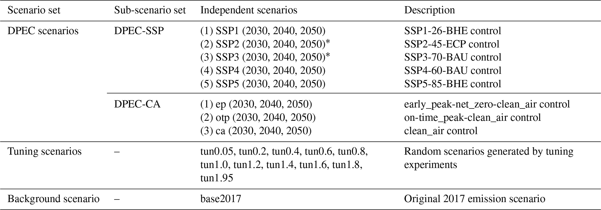
^* Samples corresponding to six scenarios from SSP2 and SSP3 in the multi-scenario dataset were utilized for model testing, whereas the remaining samples were employed for model training.

2.1.2 GEOS-Chem configuration

The GEOS-Chem chemical transport model (http://www.geos-chem.org, last access: 15 January 2025, version 14.2.2) (GC) was used to simulate the spatiotemporal distribution of surface PM_2.5 and O₃ concentrations under different emission scenarios based on year 2017. The nested model was configured with a horizontal resolution 0.5° latitude by 0.625° longitude covering China (from 17.5 to 54° N and 72 to 136° E) and 47 vertical layers. Boundary condition files for model startup were offered by 1-year global GC simulation after spin-up of 6 months with a horizontal resolution of 2° latitude by 2.5° longitude. Assimilated meteorological data from the NASA Global Modeling and Assimilation Office's Modern-Era Retrospective analysis for Research and Applications Version 2 (MERRA-2) (Gelaro et al., 2017) were selected as meteorology fields entering the model through HEMCO interface, with the 3 h temporal resolution and 0.5° × 0.625° spatial resolution. Consistent with previous studies on future air quality assessment (Shi et al., 2021; Liu et al., 2022; Wang et al., 2023a), the meteorological inputs were fixed at 2017 for all simulations in this study to isolate concentration changes attributable solely to emission variations. The Multi-resolution Emission Inventory for China (MEIC, http://meicmodel.org/, last access: 20 January 2025) (Li et al., 2017) and the multi-scenario emission inventories with a horizontal resolution of 0.25° latitude by 0.25° (as detailed in Sect. 2.1.1) were used as the monthly anthropogenic emissions to simulate PM_2.5 and O₃ concentrations under various emission scenarios. For anthropogenic emissions out of China, we used data from the Community Emissions Data System (CEDS) inventory (Hoesly et al., 2018). All the GC simulations in this research relied on identical configurations: GEOS-Chem version 14.2.2, compiled with OpenMP parallelization (OMP_NUM_THREADS = 32), executed on a Linux cluster node equipped with two Intel(R) Xeon(R) E5-2620 v4 CPUs (8 cores per socket, 32 logical processors total) and 62 GB RAM.

2.1.3 Multi-scenario dataset

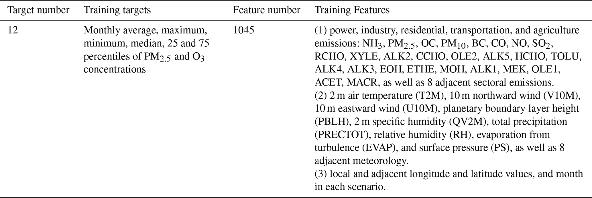
Before model training and evaluation, we constructed a multi-scenario dataset by combining emissions with the corresponding GC simulations, as summarized in Table 1. Each sample in this dataset is defined on a grid-cell basis. All emission data were interpolated to a spatial resolution of 0.5° × 0.625° to match the GC simulations. Detailed descriptions of the input features and output targets are provided in Table 2. For each grid cell, 105 sectoral emissions were selected as predictors to represent local emission conditions. At this resolution, a 3 × 3 grid domain already covers a geographic extent for representing influences of neighborhood areas towards local pollutants in a monthly scale, seeing details in Text S2. Therefore, to account for regional transport of precursors, we incorporated the emissions of the eight neighboring cells. In addition, nine key meteorological variables, previously identified as strongly correlated with PM_2.5 and O₃ concentrations (Shi et al., 2020; Zhang et al., 2022a), were included for each local and neighboring grids, based on the 2017 MERRA-2 reanalysis processed into monthly averages. Spatial information of both the local and adjacent grids was further incorporated to enable the model to capture spatial heterogeneity in emissions and pollutant concentrations. The training targets consisted of twelve statistical indicators on a monthly scale, including the 25th and 75th percentiles, median, mean, maximum, and minimum, derived from the daily averaged concentrations of PM_2.5 and O₃ in the GC outputs for each scenario. It is important to emphasize that our analysis focuses on air quality responses to anthropogenic emission changes. Consequently, dust-related components were excluded during preprocessing, since dust intrusions can introduce large predictive biases in northern and western China, where they make substantial contributions to PM_2.5 concentrations (Pang et al., 2023).

Table 2 Targets and features for TGEOS model.

2.2 Methodology

2.2.1 Model architecture

Previous emulator studies have often adopted field-based modeling strategies, in which both inputs and outputs are represented as spatially explicit two-dimensional fields (Xing et al., 2020; Huang et al., 2021; Liu et al., 2022). While effective in data-rich settings, such formulations typically require a large number of training samples to robustly learn high-dimensional spatial mappings. In the present study, the number of available scenarios is limited, yielding fewer than 500 samples in total for training. This sample size is insufficient to support stable training of high-capacity field-to-field models, particularly when the input space includes more than 100 variables spanning sectoral emissions and multiple meteorological parameters. Under this data regime, directly modeling full spatial fields would substantially increase the risk of overfitting and unstable generalization. Therefore, rather than adopting a purely field-based representation, we reformulate the problem as a high-dimensional sequential learning task. The dataset is organized as structured multivariate sequences, in which spatial and feature-level information, such as emissions, meteorology, and concentrations over a 3 × 3 neighborhood (nine grid cells), is flattened and treated as a sequence of tokens input to the TGEOS model. This formulation is better aligned with the available sample size and enables more efficient utilization of limited training data, while still preserving key spatial and cross-variable dependencies among neighboring grid points.

The TGEOS model comprises the encoder for feature extraction and the regressor for target mapping, with detailed architecture illustrated in Fig. S1. In order to align with the shape of the dataset, the model was configured with an input feature dimension of 1045 and an output dimension of 12. Six Encoder layers were configured with the model, each of which primarily incorporates a multi-head self-attention mechanism with eight attention heads and a feed-forward network. The multi-head self-attention mechanism was employed to capture the dependency relationships among various positions within the input sequence, while the feed-forward network facilitates additional nonlinear transformations on the features at each position (Vaswani, 2017). By leveraging the multi-head self-attention mechanism, the model can compute the similarity (or attention weights) of each feature in relation to all other features, thus producing a weighted representation for each position and determining the extent to which each position relies on information from others. Moreover, the feed-forward network, consisting of two fully connected layers, enhanced feature representation and improves the model's learning efficacy by incorporating nonlinear activation functions. In this implementation, the ReLU activation function was selected due to its ability to prevent negative values and expedite the model's training process (Nair and Hinton, 2010). Additionally, each sub-module incorporated residual connections and layer normalization to mitigate the risks of gradient disappearance or explosion. The output from the Encoder undergoes global pooling to decrease model complexity. Finally, the output of the encoder is transformed into the specified sequence by the regressor, which is implemented as a linear layer.

As depicted by Fig. 1, the model incorporates local and surrounding sectoral emissions for each grid, along with various meteorological parameters, to predict the probability distribution of pollutants under different scenarios, which is characterized by a series of concentration indicators including the average, maximum, minimum, median, 25 and 75 percentile of PM_2.5 and O₃. Previous research has indicated that PM_2.5 and O₃ concentrations tend to follow characteristic statistical patterns (Zhang et al., 2018; Zeng et al., 2021), with PM_2.5 generally displaying a right-skewed Gamma-like distribution and O₃ approximating a normal distribution. This distinction is also evident from the comparison of their mean and median values. Based on this insight, we used the TGEOS-predicted statistical indicators to approximate regional probability distribution curves. Specifically, the mean, 25th, and 75th percentiles were applied to capture the overall shape of the distributions, while the minimum and maximum values were incorporated to constrain their ranges.

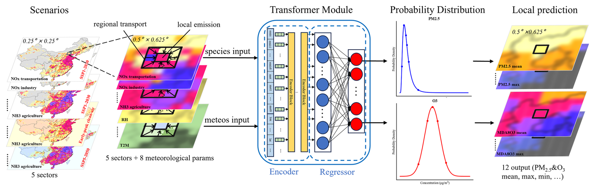
Figure 1 Workflow of TGEOS technique.

2.2.2 Model training and evaluation

In this study, four machine learning models were employed independently to evaluate the performance for each kind of model structure. Except for the TGEOS model discussed in this paper, two traditional ML models, e.g. Multilayer Perceptrons (MLP) and Random Forests (RF), as well as two advanced ones, namely Convolutional Neural Network (CNN) and Vision Transformer (ViT), which demonstrated good performance in air quality modeling (Huang et al., 2021; Fang et al., 2023; Pang et al., 2025), were simultaneously employed based on the same training set. For each model, the optimizer and loss function were identical, and hyperparameters were obtained after fine-tuning based on Optuna tool, and specific tuning schedules were listed in Tables S5 to S11 in the Supplement. Training and evaluation of these models were conducted on a GPU-equipped server. Specifically, the benchmark was measured on an NVIDIA GeForce RTX 4080 with 31 GB memory, using PyTorch 2.3.1 with CUDA 12.4 and Python 3.11.5, running under Ubuntu 20.04.6.

The detailed dataset for model construction was derived from the multi-scenario inventory presented in Table 1. Samples from a total of 29 scenarios within the multi-scenario dataset were selected to construct the training set. While samples from six scenarios of SSP2 (SSP2_30, SSP2_40, SSP2_50) and SSP3 (SSP3_30, SSP3_40, SSP3_50) that representing low and high emission scenarios relative to 2017 background scenario were chosen to construct the test set.

In order to optimize the ability of TGEOS model to reproduce GEOS-Chem simulations, the mean squared error (MSE) was adopt as the loss function that measures the squared variance between TGEOS predicted (m_i) and GC simulated (g_i) concentrations to supervise the model training.

$$\begin{array}{}\text{(1)}& \mathcal{L}\left(m\right)={\displaystyle \frac{\mathrm{1}}{N}}\sum _{i=\mathrm{1}}^N(m_i-g_i{)}^{\mathrm{2}}\end{array}$$

The model weights were optimized with respect to the loss function using the Adam optimizer (Kingma, 2014) with an learning rate is $\mathrm{1}\times {\mathrm{10}}^{-\mathrm{4}}$. To save the optimal model weights during training, 20 % of the randomly sampled training data were set aside for model validation purposes. The model was trained for 100 epochs with a batch size of 64. To reduce the risk of overfitting, we applied L2 weight regularization on all trainable parameters during training and fine-tuning.

The performance of TGEOS was evaluated using three statistical indices commonly used in evaluating the performance of CTM emulators (Salman et al., 2024), namely, coefficient of determination R-Square (R²) and Mean Absolute Error (MAE). Their corresponding mathematical formulas are delineated as follows.

$$\begin{array}{}\text{(2)}& {\displaystyle }{R}^{\mathrm{2}}=\mathrm{1}-{\displaystyle \frac{\sum _{i=\mathrm{1}}^N(m_i-g_i{)}^{\mathrm{2}}}{\sum _{i=\mathrm{1}}^N(m_i-\stackrel{\mathrm{‾}}{m}{)}^{\mathrm{2}}}}\text{(3)}& {\displaystyle }\mathrm{MAE}={\displaystyle \frac{\mathrm{1}}{N}}\sum _{i=\mathrm{1}}^N|m_i-g_i|\end{array}$$

Here m_i and g_i denote the TGEOS-predicted and GC-simulated pollutant concentrations, respectively. Indices i means the ith grid cell. $\stackrel{\mathrm{‾}}{m}$ is the average of all the model-predicted samples and N refers to the number of samples from the training set.

3 Results and discussions

The overall performance of TGEOS on the test set is shown in Table S1. We found that the model performed well across all target indicators. The R² ranges from 0.958 to 0.992, with relatively low RMSE and MAE, averaging 2.808 and 1.588 µg m⁻³, respectively. The following presents detailed analyses: Sect. 3.1 focuses on analyzing the differences between the training set and the test set; Sect. 3.2 and 3.3 involves predicting spatial and probability distributions of PM_2.5 and O₃ concentrations; Sect. 3.4 is dedicated to comparison of different models.

3.1 Differences between training and test set

Since emission trajectories with different reduction rates may converge at certain time horizons, there exists a potential risk of data leakage arising from similarities in emission and concentration levels across scenarios. To address this concern, we analyzed the Kernel Density Estimation (KDE) curves for six key emission variables, which strongly influence PM_2.5 and O₃ concentrations (Hu et al., 2023), of the training and test set, as illustrated in Fig. S5. The results indicate that, although the general distribution trends are similar, the densities at different emission levels vary significantly between the two. Furthermore, focusing on the North China Plain (NCP) where both PM_2.5 and O₃ pollution are particularly severe, we examined the spatial distribution of mean PM_2.5 and O₃ concentrations, six critical emissions as well as corresponding absolute differences under the stochastically selected SSP2_2050 test scenario, in comparison with a training scenario (otp2030). The otp2030 scenario was selected by calculating the Euclidean distance between the mean PM_2.5 and O₃ values of SSP2_2050 and those of each training scenario, and identifying the scenario with the minimum distance. The results are illustrated in Fig. 2 for PM_2.5 and Fig. S4 for O₃. These pictures indicated that the concentrations of pollutants, as well as emission variables, of the training and test set are exclusive despite some distributional similarities, particularly for samples from highly polluted regions.

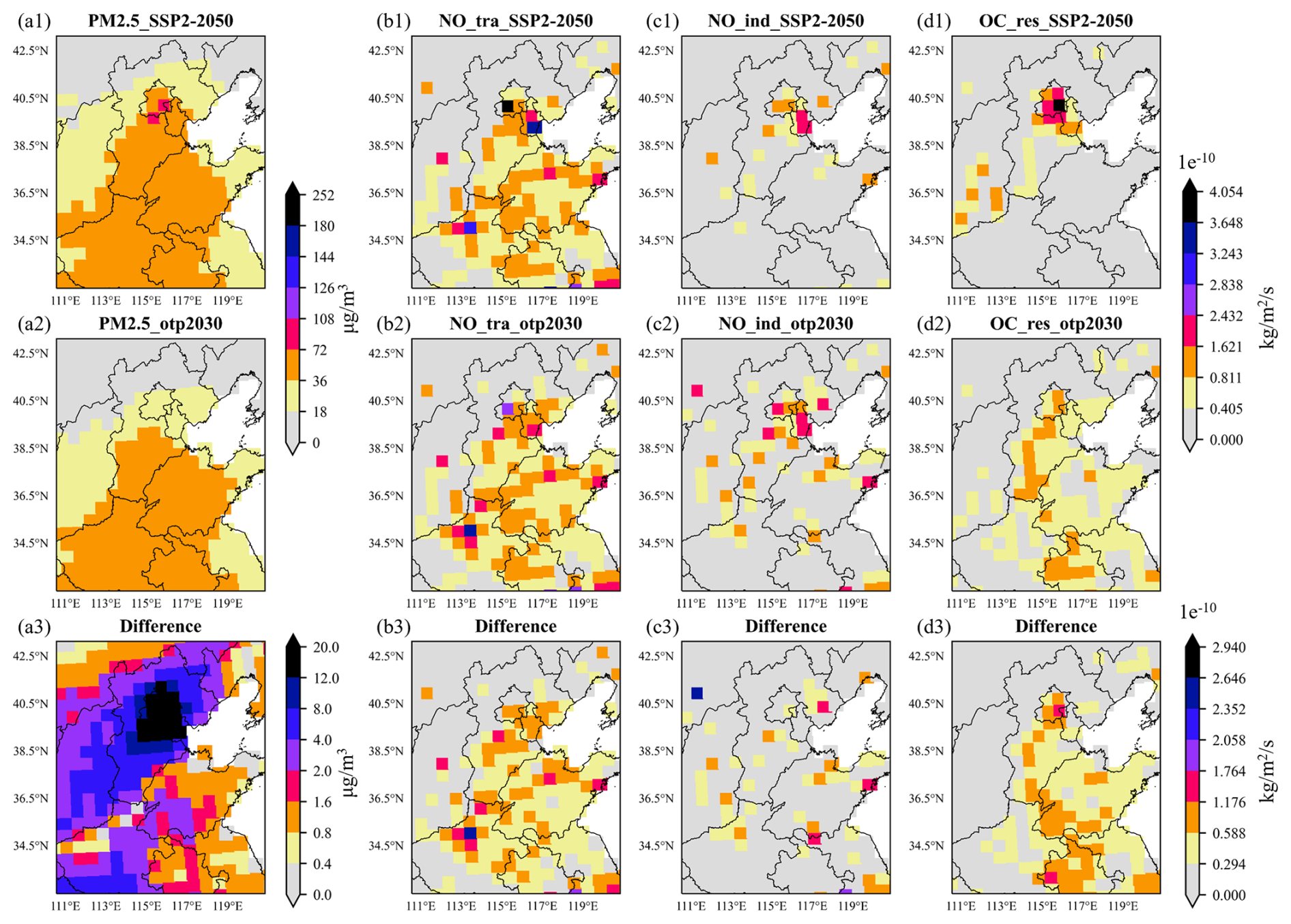
Figure 2 Spatial distributions of mean PM_2.5 concentration and three emission variables in SSP2_2050 (a) and otp2030 (b) scenarios in January, along with the quantified absolute differences between two scenarios (c).

In addition, we conducted Kolmogorov-Smirnov (K-S) tests on a total of 12 emission variables, comprising the aforementioned six emissions as well as an additional set of six emissions, with the results summarized in Table S4. Given the large sample size, the p-values for all emission variables are approximately zero (Demir, 2022), making the KS statistic (D-value) a more meaningful indicator. Our analysis shows that the emissions of the two scenarios differ to varying extents, with all D values being greater than zero. It is noteworthy that emission changes are primarily concentrated in major emission regions of eastern China, whereas in many western and southern regions the variations across scenarios are negligible. This spatial heterogeneity implies the presence of redundant samples in the dataset, which could in turn contribute to statistical similarities between scenarios when comparisons are made (D-value < 0.3). Nevertheless, for most emission variables, D values exceed 0.1, suggesting that certain differences still exist between the two scenarios.

3.2 Prediction of spatial distribution of PM_2.5 and O₃

We first evaluated the spatial distribution performance of TGEOS predictions of PM_2.5 and O₃ for 6 test scenarios. For the sake of brevity, we presented the results of two test scenarios, namely SSP2_2040 and SSP3_2040, to represent the low and high emission scenarios. Additionally, we focused on the months with the highest concentrations of PM_2.5 and O₃ to better visualize the spatial distribution of pollutants. Figures 3 and S6 present the spatial comparison of PM_2.5 concentration indicators between GC and TGEOS for SSP2_40 and SSP3_40 scenario in January.

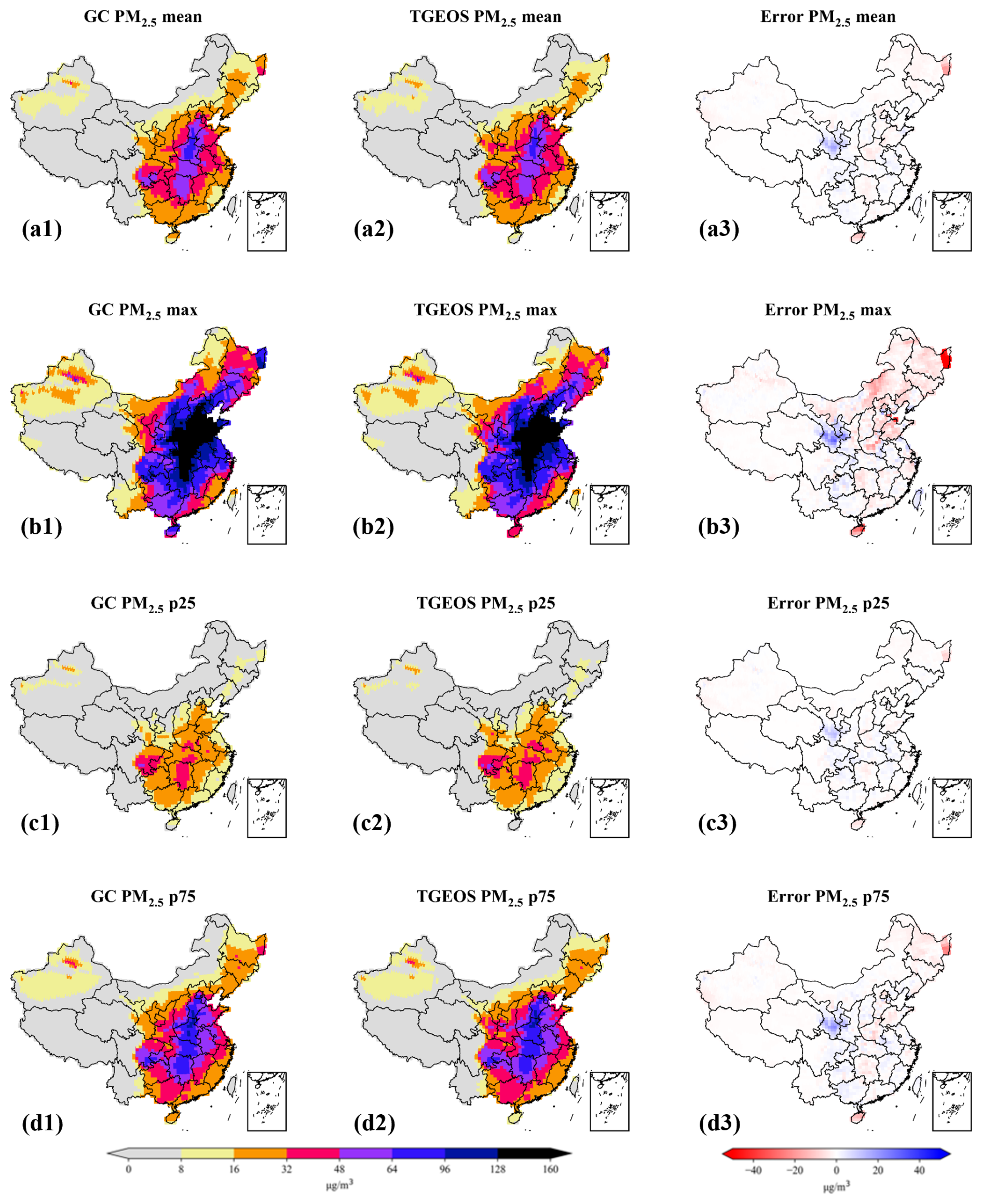
Figure 3 Spatial comparison of GEOS-Chem simulated and TGEOS estimated four statistical indicators of PM_2.5 concentrations in January under SSP2_2040 scenario (low emissions) and the corresponding error maps. Panels (a1) to (d1) represent GC simulation while (a2) to (d2) represent TGEOS prediction, and (a3) to (d3) represent the error between this two for each indicator, including mean, maximum, 25-percentile, and 75-percentile.

The results demonstrate that, across various emission scenarios, the spatial distribution of PM_2.5 concentrations simulated by TGEOS exhibits a high degree of similarity with that produced by GC. Specifically, TGEOS effectively captures the spatial distribution patterns of PM_2.5 concentrations, accurately identifying high-pollution zones in central and northern China, alongside low-pollution areas in other regions. Furthermore, the disparities observed in PM_2.5 concentration levels under distinct emission scenarios indicate that TGEOS has successfully discerned the intricate relationships between precursor emissions and PM_2.5 concentrations. Beyond its capability to predict monthly mean values, TGEOS also excels in predicting additional statistical indicators associated with PM_2.5 concentrations, including the maximum concentrations of significant concern to policymakers as well as the 25th and 75th percentile, which reflect the distribution of concentrations. Other statistical indicators, such as the median and minimum values that shown in Fig. S8, are also effectively predicted.

As illustrated in Figs. 5a, 6a, and S10a, there exists a robust statistical correlation between the PM_2.5 indicators predicted by TGEOS and the actual GC simulations across varying emission scenarios, with R² values ranging from 0.976 to 0.995. These results substantiate that PM_2.5 accurately captures the principal trends and patterns of PM_2.5 as simulated by GC. The evaluation of model prediction errors, as quantified by the RMSE and MAE, reveals relatively low error levels, with RMSE values ranging from 0.985 to 2.110 and MAE values between 0.685 and 3.243, demonstrating the predictive capabilities of TGEOS with a high degree of accuracy and reliability. The MBE values are ranging from −1.453 to 1.420 for PM_2.5, −0.033 to 1.125 for O₃, indicating a slight overall deviations in concentration predictions compared to corresponding GC simulations. Considering that this bias is relatively small compared to the magnitude of the concentrations, the model can be regarded as nearly unbiased. In addition, to evaluate the capability of TGEOS in capturing extreme events, we employed exceedance metrics based on the 90th percentile threshold of the concentration distribution. The results indicate that the model achieves high precision and recall score for both PM_2.5 and O₃ indicators, with all these values larger than 0.85. These values suggest that the majority of the predicted exceedance events correspond to actual exceedances, while nearly all true exceedance events are successfully detected. The high and balanced values of both metrics demonstrate that TGEOS is capable of accurately identifying extreme high-value occurrences with low false alarm and miss rates. Moreover, this performance highlights the robustness of the model in reproducing the upper tail of the distribution, which is particularly important for applications focusing on extreme pollution events.

The spatial comparison of O₃ concentration indicators between GC and TGEOS for two scenarios in July are presented in Figs. 4, S7, and S9. Similar to the predictions for PM_2.5, we observed that TGEOS successfully captures the spatial distribution patterns of O₃ as simulated by GC, as well as the concentration differences resulting from various emissions. The scatter density plots presented in Figs. 5b, 6b, and S10b indicate a strong correlation between TGEOS and GC, with R² values ranging from 0.966 to 0.996. Additionally, the accuracy of TGEOS predictions is further supported by the relatively low RMSE values, which range from 0.985 to 2.110, and MAE values ranging from 1.593 to 4.933. These results demonstrate that TGEOS is capable of accurately and reliably predicting both PM_2.5 and O₃ concentration distribution across different scenarios, achieving a level of performance comparable to that of GC.

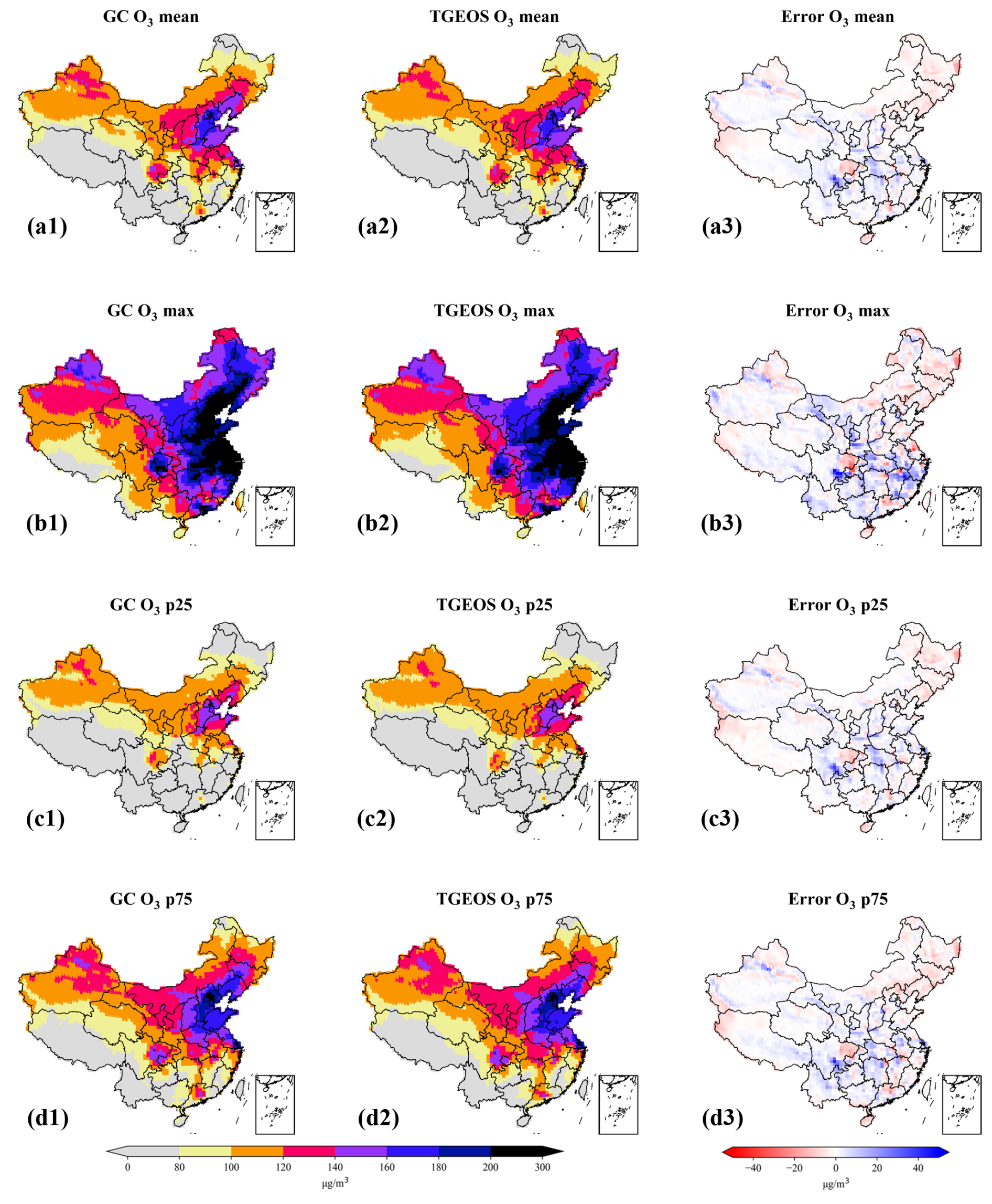
Figure 4 Spatial comparison of GEOS-Chem simulated and TGEOS estimated four statistical indicators of O₃ concentrations in July under SSP2_2040 scenario (low emissions) and the corresponding error maps. Panels (a1) to (d1) represent GC simulation while (a2) to (d2) represent TGEOS prediction, and (a3) to (d3) represent the error between this two for each indicator, including mean, maximum, 25-percentile, and 75-percentile.

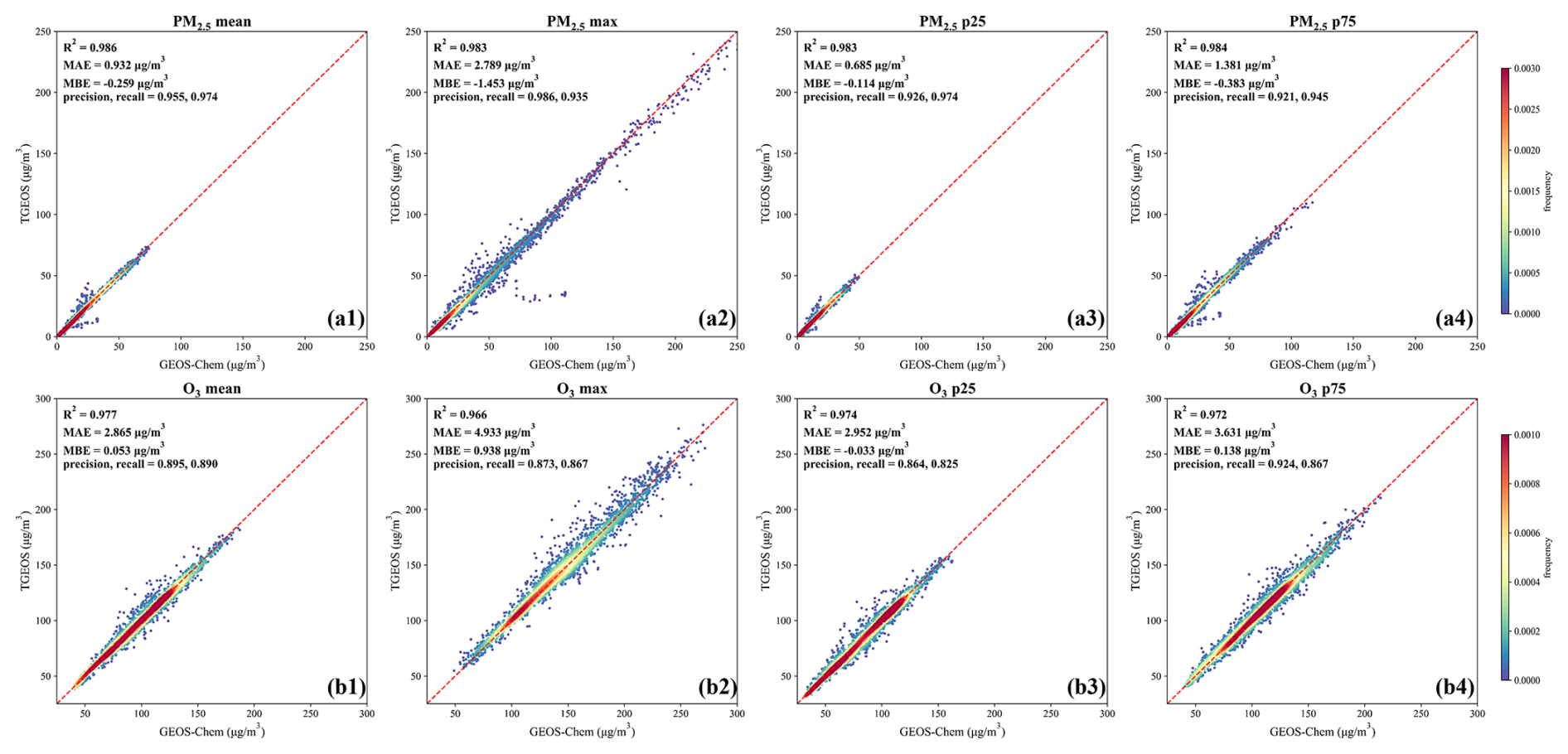
Figure 5 Density scatter plots between GEOS-Chem simulations and TGEOS predictions for eight indicators of PM_2.5 (a) and O₃ (b) concentrations in SSP2_2040 scenario. Panels (a1) to (a4) denote the mean, maximum, 25th percentile, and 75th percentile of January PM_2.5 concentration; (b1) to (b4) denote the corresponding statistics for July O₃ concentration.

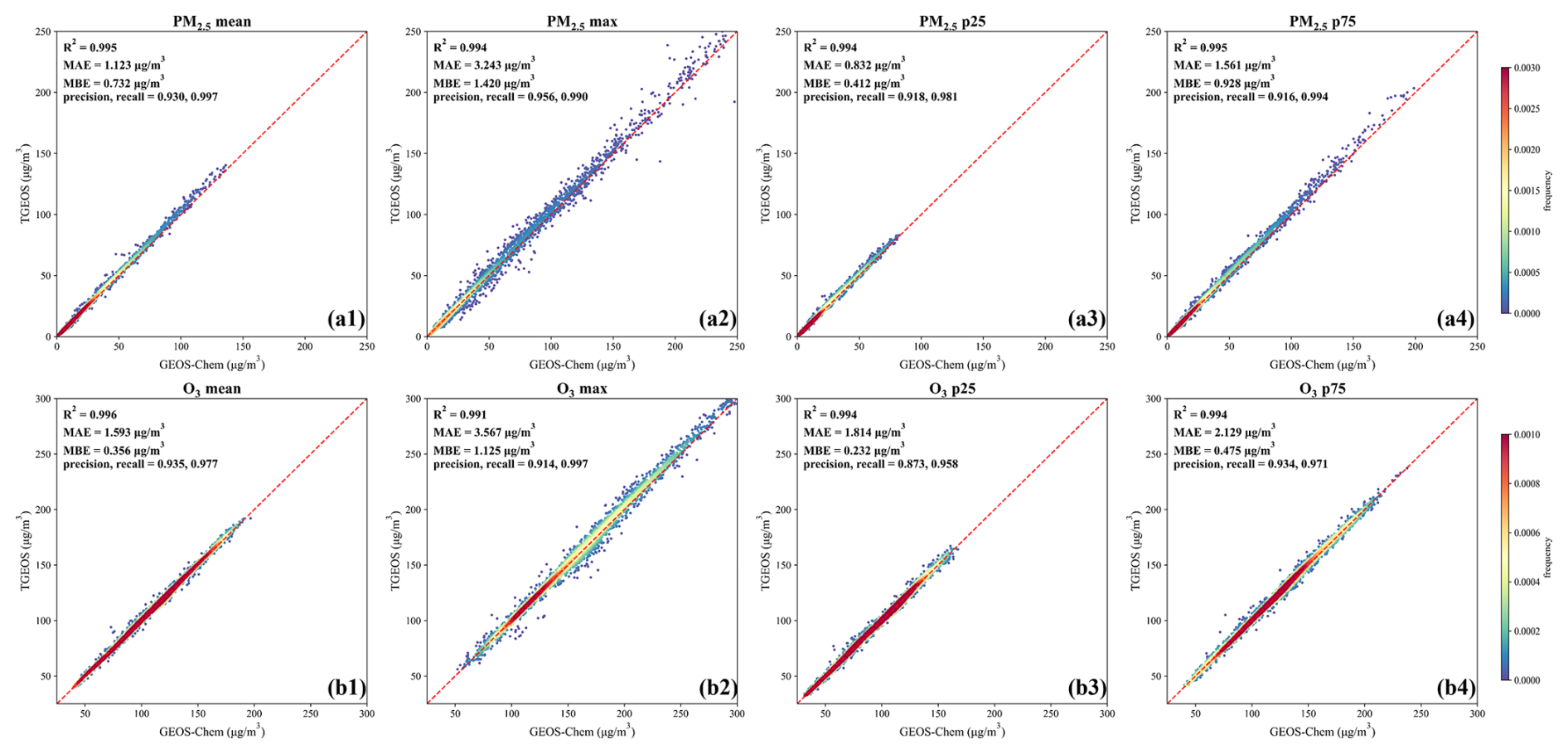
Figure 6 Density scatter plots between GEOS-Chem simulations and TGEOS predictions for eight indicators of PM_2.5 and O₃ concentrations in SSP3_2040 scenario. Panels (a1) to (a4) denotes the mean, maximum, 25th percentile, and 75th percentile of January PM_2.5 concentration; (b1) to (b4) denotes the corresponding statistics for July O₃ concentration.

The error graphs of PM_2.5 indicators for SSP2_2040 and SSP3_2040 are shown in Figs. 3a3 to d3 and S6a3 to d3. We found the model exhibits relatively large errors in predicting the monthly maximum concentrations of PM_2.5. This is attributed to the inherent randomness of these peak values compared to other indicators, which poses challenges for accurate prediction. Furthermore, our analysis indicates the presence of both overestimation and underestimation within these error graphs. In this study, the GC simulations for each scenario were initialized from a fixed concentration field derived from the 2017 background scenario. As monthly concentrations were treated as independent and did not incorporate the influence of initial fields, discrepancies may arise between model predictions and GC outputs, especially when future concentration levels deviate substantially from the initial state. This effect helps explain the relatively poorer predictive performance under SSP2 scenarios (Fig. 5), as well as the observed patterns of systematic over- and underestimation in the error distributions. Specifically, in the SSP2 scenario (SSP2-45-ECP), stringent environmental policies are projected in the short and medium term (Tong et al., 2020), thereby widening the gap between future and historical emissions and amplifying predictive errors, particularly during the early simulation period. In contrast, under the SSP3 scenario (SSP3-70-BAU), characterized by pessimistic development trajectories and limited investments in environmental protection (Tong et al., 2020), emissions are projected to change slightly, resulting in smaller differences from historical conditions (Fig. 6). Consequently, predictions in SSP3 scenarios are less affected by initialization effects than those in SSP2.

The predictions from TGEOS also demonstrate a clear pattern of seasonal variation. Here, we focus on two statistical indicators that are crucial for fitting the probability distribution curve, namely the 25th percentile and the 75th percentile, and select results from January, April, July, and October to represent the distribution of pollutants during winter, spring, summer, and autumn, respectively. Figures 7 to 8 and S15 to S16 illustrate the seasonal variation of PM_2.5 and O₃ indicators predicted by GC and TGEOS under SSP2_2040 and SSP3_2040 scenarios. The R² values for the 25th and 75th percentile of PM_2.5 are 0.964 to 0.994 and 0.973 to 0.996, respectively, while those for O₃ are 0.903 to 0.994 and 0.946 to 0.994, respectively, indicating a strong correlation between predicted and simulated pollutant concentrations across all seasons.

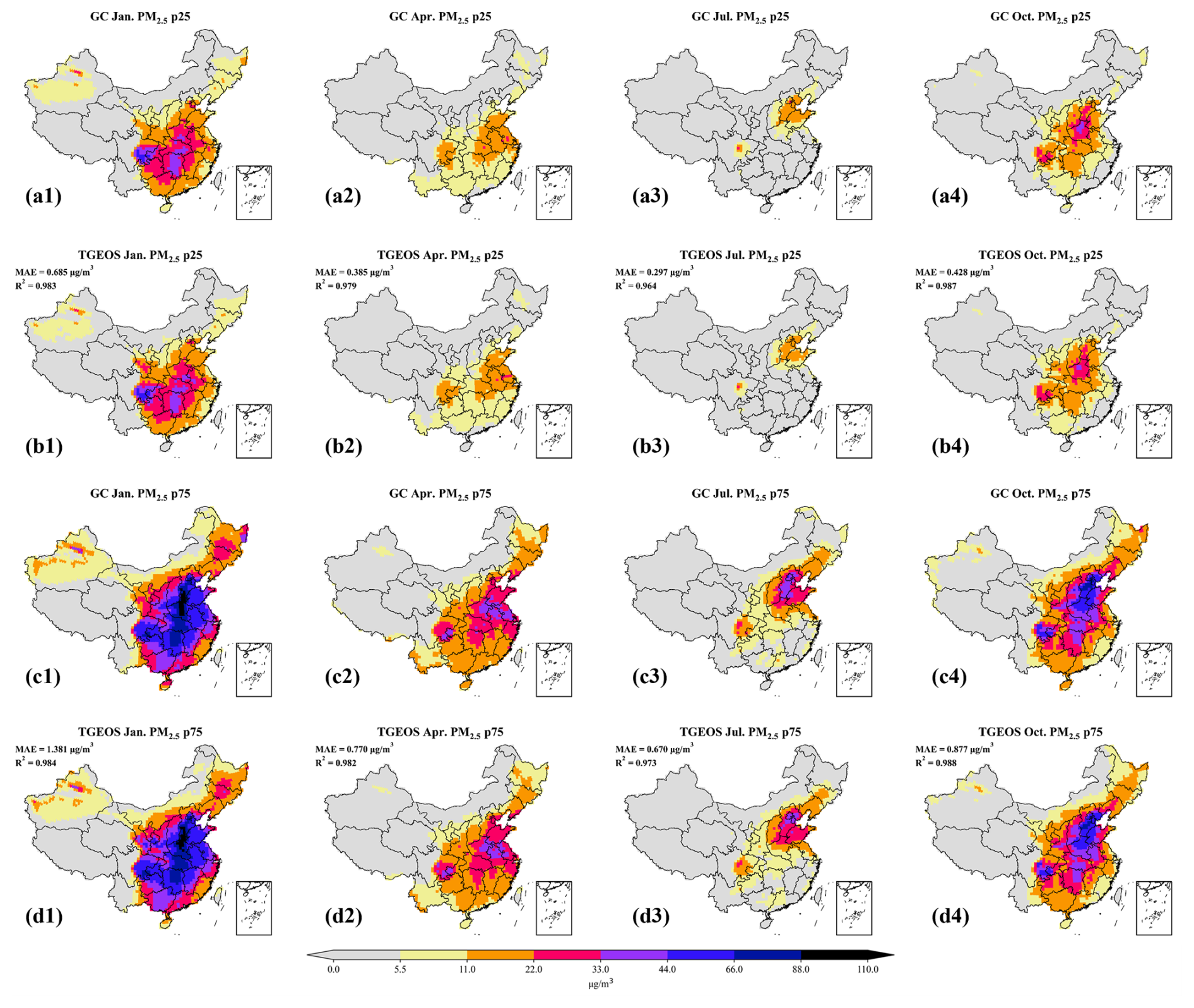
Figure 7 Spatial distribution of 25th and 75th percentile of PM_2.5 concentrations estimated by GEOS-Chem and TGEOS in January, April, July and October under SSP2_2040 scenario. Panels (a) and (c) illustrate the GEOS-Chem simulations for the 25th and 75th percentile of PM_2.5 from January to October. Panels (b) and (d) depict the TGEOS estimates for the 25th and 75th percentile of PM_2.5 concentrations during the same months.

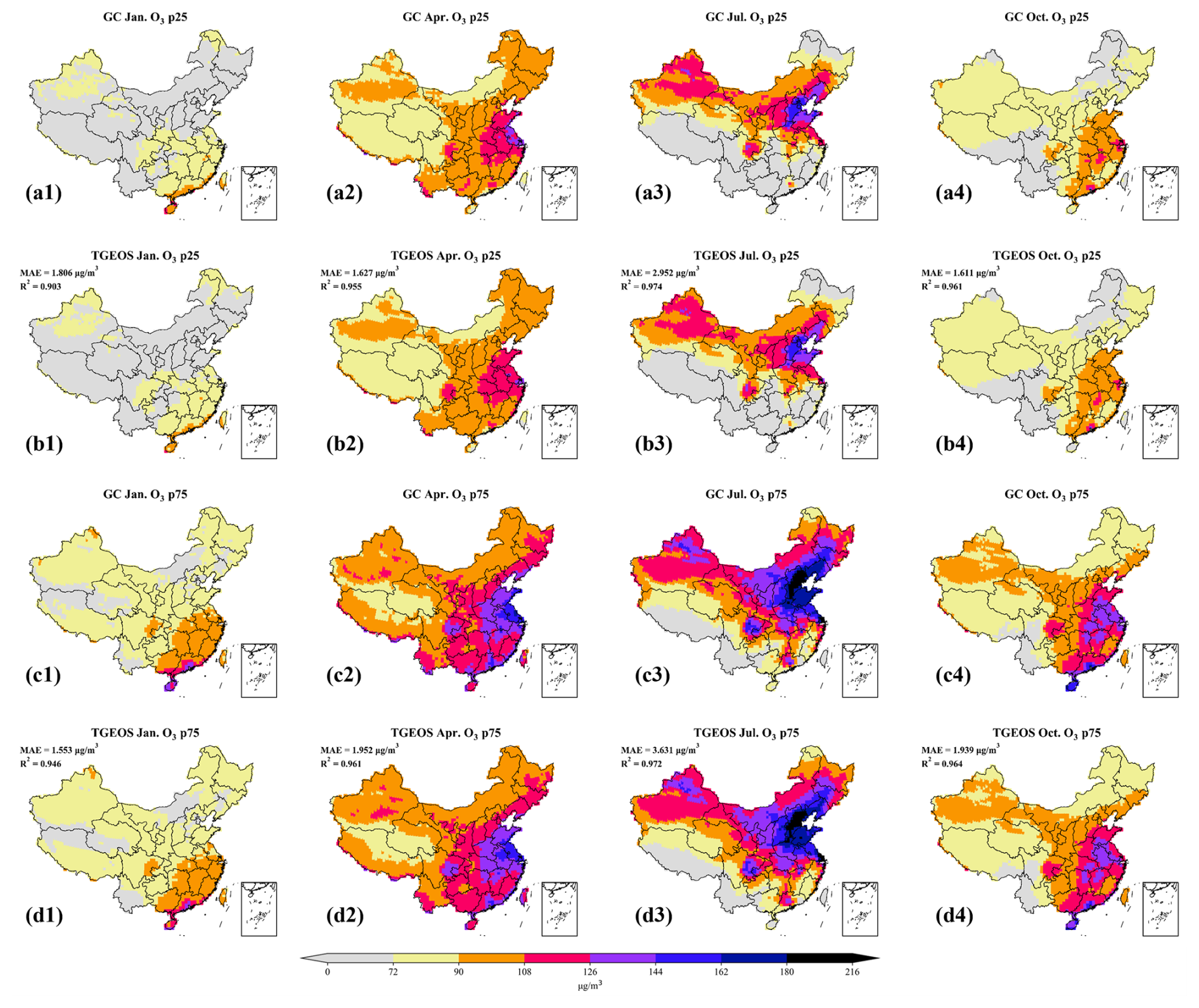
Figure 8 Spatial distribution of 25th and 75th percentile of O₃ concentrations estimated by GEOS-Chem and TGEOS in January, April, July and October under SSP2_2040 scenario. Panels (a) and (c) illustrate the GEOS-Chem simulations for the 25th and 75th percentile of O₃ from January to October. Panels (b) and (d) depict the TGEOS estimates for the 25th and 75th percentile of O₃ concentrations during the same months.

Specifically, TGEOS effectively captures the seasonal trends and patterns of PM_2.5 and O₃ as simulated by GEOS-Chem. Seasonal variations in both pollutants are evident, with PM_2.5 concentrations gradually decreasing from winter to summer (Figs. 7.1 to 3 and S15.1 to 3), while O₃ concentrations exhibit a gradual increase during the same period (Figs. 8.1 to 3 and S16.1 to 3). Furthermore, the accuracy of TGEOS predictions is noteworthy, as evidenced by the low MAE values for the 25th and 75th percentiles of PM_2.5 (0.297 to 0.832 and 0.670 to 1.561, respectively) and O₃ (1.186 to 2.952 and 1.186 to 3.631), indicating that TGEOS predictions closely align with GC simulations, despite some acceptable margin of error. Although the performance during periods of low concentration was less optimal, TGEOS demonstrated decent effectiveness during critical months when elevated concentrations and extreme pollution events are more likely to occur, particularly for PM_2.5 in January and O₃ in July.

From the perspective of predicting the spatial distribution of pollutants, although some discrepancies exist, TGEOS exhibits relatively high accuracy and reliability in predicting PM_2.5 and O₃ concentrations during key pollution months and across various seasonal pollution conditions compared to the corresponding simulations from GC.

3.3 Prediction of probability distribution of PM_2.5 and O₃

The probability distribution offers a comprehensive representation of pollutant concentrations over a specified time period and effectively captures extreme values, which are typically reflected in the tails of the probability distribution curve. Leveraging this advantage, probability distributions are critical in various air pollution studies, including investigations into future air quality under different emission scenarios (Zeng et al., 2022) or climate changes (Li et al., 2024), and potential mortality in heavily polluted regions (Tian et al., 2022). In this study, we focus on the probability distributions predicted by TGEOS for four key polluted areas: the North China Plain (NCP, 34–42° N, 113–120° E), Yangtze River Delta (YRD, 26–34° N, 115–123° E), Fenwei Plain (FWP, 33–38° N, 103–114° E), and Sichuan Basin (SCB, 26–34° N, 103–107° E). For each region, the probability density function (PDF) curves were fitted using the TGEOS-predicted monthly indicators averaged over all grid cells in the region. For PM_2.5, we fitted a right-skewed gamma distribution; for O₃, we fitted a normal distribution. The fitting procedure primarily used the 25th percentile, 75th percentile, and mean as parameters to characterize the distribution shape, with the maximum and minimum values used to constrain the distribution boundaries. These probability distribution curves derived from monthly statistical indicators can be used to preliminarily assess the overall distribution of pollutant concentrations for a given month or quarter under various future emission scenarios.

The PM_2.5 concentration distributions from GC simulations and TGEOS predictions for the NCP, YRD, FWP, and SCB in SSP2_2040 and SSP3_2040 are illustrated in Fig. 9. Additional results, encompassing four scenarios for the years 2030 and 2050, are presented in Figs. S17 and S19. We found the probability distribution curves of PM_2.5 concentration that TGEOS predicted in these regions exhibit a strong correlation with corresponding GC curves, indicating that TGEOS model has successfully established the relationship between PM_2.5 concentration and emissions of precursors in different regions for varying scenarios. The effects of different emission scenarios are clearly reflected. We found that in low-emission scenarios (panels a1 to d1), the PM_2.5 probability curves for all four regions exhibited significant changes. The reduction in precursor emissions led to a decrease in overall PM_2.5 concentrations, resulting in an increase in lower values. This caused the peak of the curve to shift to the left relative to the base curve and become sharper. In contrast, in high-emission scenarios (panels a2 to d2), the increase in precursor emissions resulted in higher PM_2.5 concentrations, shifting the peak to the right and displaying a trend towards flattening.

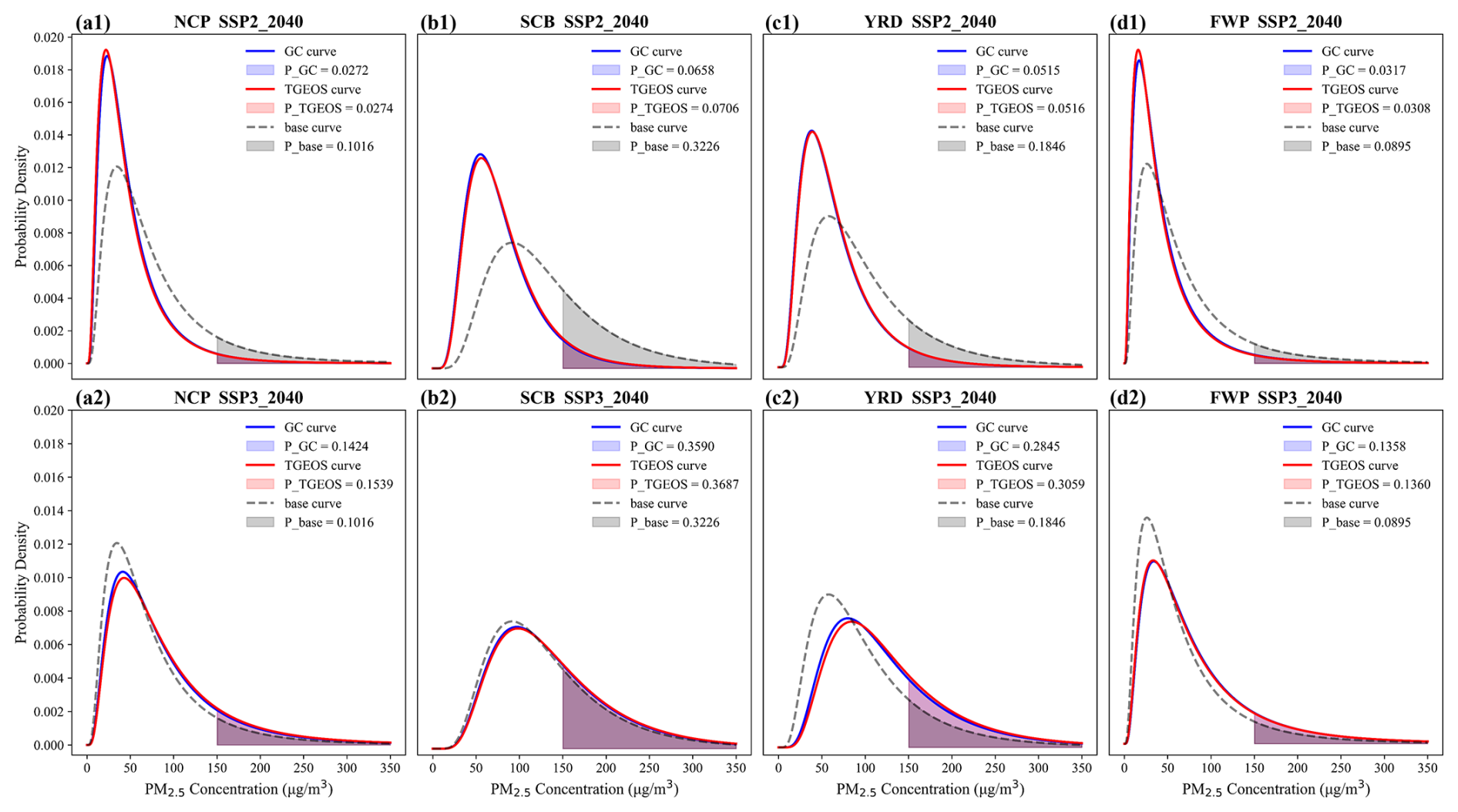
Figure 9 Probability distribution curves of winter PM_2.5 fitted by GC and TGEOS estimates under two scenarios (SSP2_2040 and SSP3_2040) in four interest regions, including NCP (a), SCB (b), YRD (c), and FWP (d). The blue solid line and the red solid line represent the probability distribution curve of GC and TGEOS results. The black dashed line shows the distribution of pollutants in 2017 (background scenario). P_GC, P_TGEOS and P_base represent the probability of extreme pollution events (calculated from colored areas of each curve) in GC simulation, TGEOS prediction, and 2017 simulation.

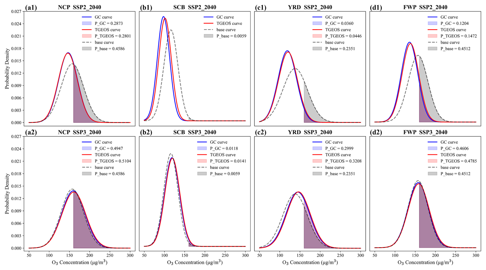
Figure 10 Probability distribution curves of summer O₃ fitted by GC and TGEOS estimates under two scenarios (SSP2_2040 and SSP3_2040) in four interest regions, including NCP (a), SCB (b), YRD (c), and FWP (d). The blue solid line and the red solid line represent the probability distribution curve of GC and TGEOS results. The black dashed line shows the distribution of pollutants in 2017 (background scenario). P_GC, P_TGEOS and P_base represent the probability of extreme pollution events (calculated from colored areas of each curve) in GC simulation, TGEOS prediction, and 2017 simulation.

Figures 10, S18, and S20 illustrate the O₃ concentration distributions predicted by TGEOS for NCP, SCB, YRD, and FWP. Similar to PM_2.5, the probability distribution curves of O₃ predictions show good agreement with GC curves. TGEOS also established the relationship between O₃ concentrations and emissions in these regions, and successfully predicted the probability distribution of concentrations under various test scenarios. In high emission scenarios, excessive precursor emissions elevate overall O₃ pollution levels, resulting in the occurrence of more high-value concentrations. This flattens the distribution curve of O₃ compared to the base curve, while also lowering its peak value. Conversely, in low emission scenarios, the reduction of precursor pollutants – such as nitrogen oxides (NO_x) and volatile organic compounds (VOC_s), which significantly influence O₃ formation – leads to a decrease in O₃ concentration. This also sharpens the O₃ distribution curve and enhances its peak value. Since the meteorological conditions for all scenarios are fixed in 2017, both concentration variations of PM_2.5 and O₃ can be attributed to changes in emissions.

Additionally, we observed that the model performs slightly poorly in predicting the probability distribution of pollutants under certain high emission scenarios like Figs. S17 and S20 (panels a2 to d2). As discussed in Sect. 3.3, this discrepancy arises from the limited number of high-emission samples in the dataset, which undermines the model's generalization capabilities. It is also important to emphasize that when predicting O₃ levels under the SSP2_2050 scenario, TGEOS shows a clear underestimation in the YRD region (Fig. S20d1). To investigate this, we compared the emission distributions of SSP2_2050 and the training set. As shown in Fig. S21, several precursor emissions (e.g., CO residential, NO transportation) exhibit much higher densities in the low-emission range under SSP2_2050 (orange line) than in the training set (blue line), where the model has limited training experience. Residual analysis further confirms that the mean residuals of multiple residential emissions (CO, BC, PM_2.5, PM₁₀, SO₂) are significantly below zero in this regime (Fig. S22), consistent with their density distributions. We therefore attribute the underestimation of O₃ to distributional shifts between training and test data rather than to the direct physical or chemical effects of these species. In particular, the SSP2_2050 scenario contains a substantially larger fraction of samples in the low-emission regime, forcing the model to extrapolate beyond its well-constrained domain and regress toward mean patterns learned from the training set, thereby inducing these prediction biases.

Furthermore, we utilized TGEOS to predict the probability of extreme pollution events under various emission scenarios. According to the China National Ambient Air Quality Standard (GB3095-2012), we set 150 and 160 µg m⁻³ for PM_2.5 and O₃ concentrations as thresholds of extreme pollution events, and then calculated the probability of exceeding these thresholds by integrating the fitted probability density functions to the right, represented by the shaded areas shown in the previous images. In the graphs depicting extreme events, the probability of extreme events calculated using the TGEOS curve (represented by the red shaded area) closely matches the probability calculated using the GC curve (represented by the blue shaded area). This concordance demonstrates that TGEOS has effectively learned the distribution patterns of high-concentration pollutants and its capability to predict potential extreme pollution events under future emission scenarios.

Our findings indicate that under low-emission scenarios, the incidence of extreme PM_2.5 events decreased most significantly in the SCB and YRD regions, as illustrated in Fig. 9b1 and c1. Compared to the background scenario, the incidence in the SCB region decreased by 23.0 %, 25.2 %, and 27.4 %, while in the YRD region, it decreased by 18.1 %, 19.6 %, and 20.6 %, respectively. This indicates that implementing precursor emission reductions in these two regions can effectively control the occurrence of extreme PM_2.5 events. In contrast, under high-emission scenarios, the increase in incidence for each region was relatively small, approximately 4 % to 5 %. For extreme O₃ events, the reduction effects were most pronounced in the NCP and FWP regions. As presented in panels (a1) and (d1) of Fig. 10, under the three low-emission scenario SSP2 scenarios, the incidence of extreme O₃ events in the NCP region decreased by 17.7 %, 19.9 % and 22.8 %, while in the FWP region, it decreased by 18.6 %, 23.4 % and 27.7 %, respectively. Furthermore, as shown in panel (c1), the YRD region experienced a reduction of approximately 18 %. This demonstrates that precursor emission reductions in areas with high O₃ pollution are highly effective. Conversely, when emission levels increase, the risk of extreme O₃ events in these high-pollution regions rises sharply. Under the three high-emission scenario SSP3 conditions, the risk of extreme O₃ events in the YRD region increased by 12.8 %, 13.3 % and 14.9 %, while in the FWP region, it increased by 8.2 %, 9.7 % and 10.6 %. The changes in the NCP region were less noticeable.

The results above illustrate the impact of different emission scenarios on pollutant concentrations. Under consistent meteorological conditions, significant changes in the concentration distribution of both pollutants can be achieved through straightforward emission reductions, which notably mitigates extreme pollution risks in several heavily polluted areas. Therefore, it is essential to develop strategies to address the current state of air pollution. Furthermore, the TGEOS model shows a high level of similarity to the GC model in predicting pollutant distribution and extreme events, making it a valuable tool for online assessments of related emission reduction policies to enhance decision-making efficiency.

3.4 Comparison of different machine learning models

To validate the performance of the TGEOS model in “emission-concentration” modeling against other machine learning models, four widely used machine learning frameworks, namely Multilayer Perceptrons (MLP), Random Forests (RF), Convolutional Neural Network (CNN), and Vision Transformer (ViT) employed in previous studies (Xing et al., 2020; Huang et al., 2021; Pang et al., 2025), were simultaneously employed based on the multi-scenario dataset mentioned in Sect. 2.1. The MLP model uses 4 hidden layers with 2048, 1024, 512, and 256 neurons, applying ReLU activation and Dropout to prevent overfitting. The RF model uses 300 trees with a maximum depth of 25, a minimum sample split of 4, and a minimum sample per leaf of 2. It uses parallel computation with all CPU cores and performs feature selection by choosing the top 500 important features. The CNN model uses two 3×3 convolutional layers with ReLU activation, followed by adaptive pooling to 29×3. A month embedding is concatenated with the flattened pooled features and passed through three fully connected layers with ReLU applied to the first two. In the ViT model, the 3×3 grid cells are treated as spatial patches; a lightweight CNN is used to generate patch-level embeddings (Wang et al., 2022; Yao et al., 2024); a month token functions as a global CLS token; and the resulting token sequence is then processed by a multi-layer Transformer encoder. It should be noticed that the model inputs for CNN and ViT were reshaped from (1 × 1045) to ($\mathrm{3}\times \mathrm{3}\times \mathrm{116}$) to cater to model architecture, with specific description shown in Fig. S25.

Tables S2 and S3 summarize the performance of the five models on the entire test set. We found that TGEOS outperforms the other four models in both R² and MAE metrics. To clearly illustrate the predictive performance of different models, we presented a modified Taylor diagram (Taylor, 2005; Fang et al., 2023) in Fig. 11. This diagram simultaneously displays the Mean Absolute Error (MAE) and correlation coefficient (R) for predictions of PM_2.5 and O₃ indicators from four models in China domain. Our findings indicate that the RF model performs the poorest. This is primarily due to its reliance on feature importance assessments during feature selection, which overlooks potential underlying features in the data, adversely affecting the model's fitting capability. Additionally, the RF model is sensitive to the distribution of training data, leading to limited extrapolation abilities and poor predictive performance for extreme values. In contrast, the MLP shows a significant improvement in predictive performance relative to the RF model. Leveraging its multi-layer neural network structure, the MLP can more effectively learn complex relationships between multiple features. But this layered structure can struggle when dealing with high-dimensional feature spaces, especially for highly stochastic indicators such as maximum values, where the MLP still exhibits considerable prediction errors. Compared to MLP and RF models, models based on CNN and ViT frameworks demonstrate better performance, characterized by higher R values as well as lower MAE. However, these models still perform badly for the prediction of indicators reflecting extreme pollutant events such as 75-percentile and maximum, which is mainly because the available spatial information (3×3 grid) is inherently insufficient for these architectures relying heavily on rich spatial structure.

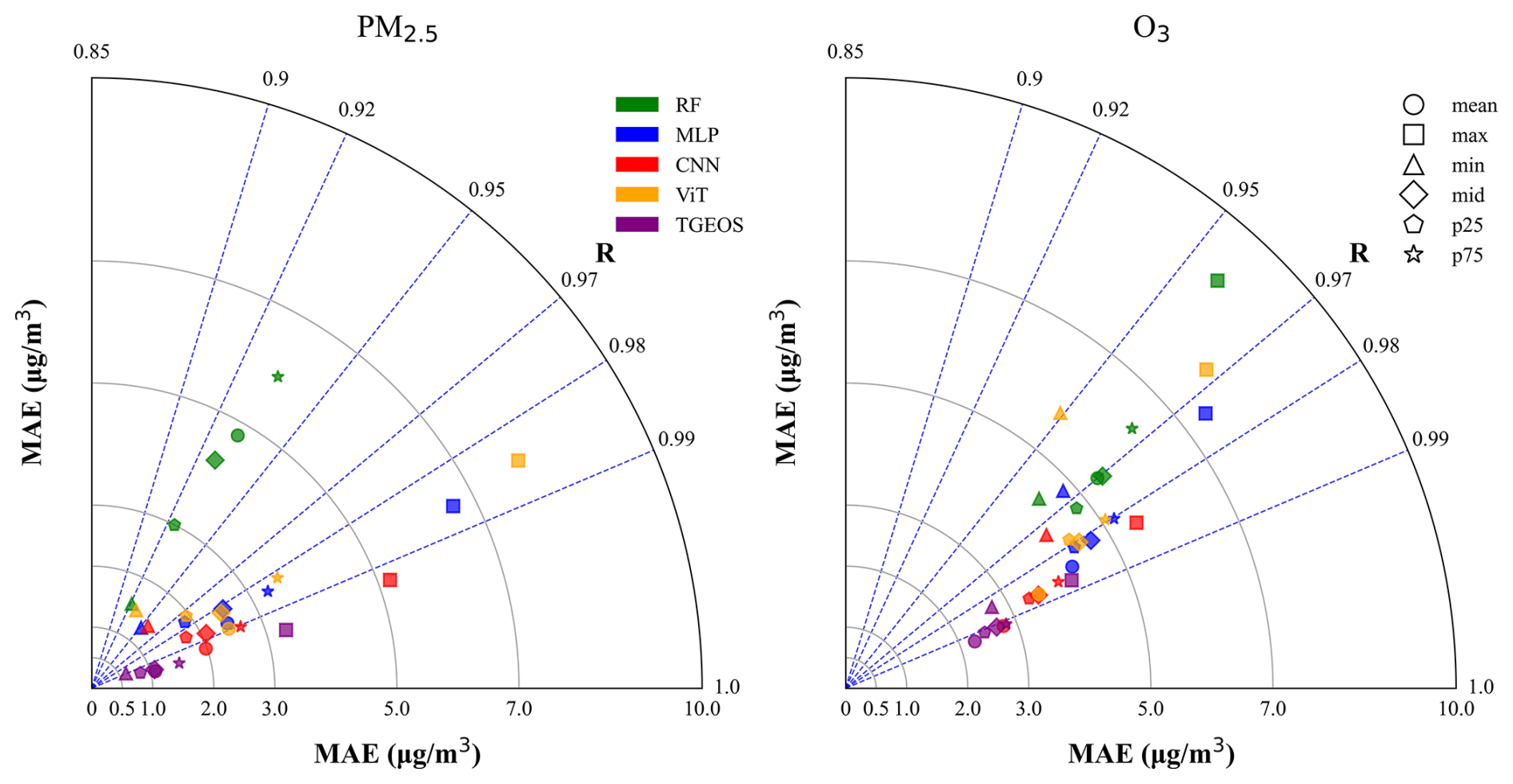
Figure 11 A modified Taylor diagram is presented to jointly illustrate the Mean Absolute Error (MAE) and correlation coefficient (R). The concentration indicators are distinguished using unique markers: circle for mean, square for max, triangle-up for min, diamond for median, pentagon for 25 percentile, and star for 75 percentile. Furthermore, the concentration indicators of winter PM_2.5 and summer O₃ predicted from different models are visualized using distinct colors, where green represents RF, blue denotes MLP, red indicates CNN, orange means ViT, and purple refers to TGEOS predictions. All indicators are computed based on the six test scenarios.

Conversely, the Transformer-based TGEOS model demonstrates superior performance compared to the other models, exhibiting higher R values (exceeding 0.98 and 0.97) and lower MAE values (less than 2.0 and 3 µg m⁻³ for the majority indicators of PM_2.5 and O₃, respectively). These results suggest a higher degree of reliability and accuracy in its predictions. For several indicators where other models perform poorly, such as the maximum, TGEOS demonstrates substantial improvements. The superiority of the Transformer model can be attributed to its greater number of parameters and more complex architecture, which leverage powerful feature extraction capabilities and self-attention mechanisms, allowing it to capture complex relationships in the high-dimensional feature space. It is worth emphasizing that although the capacity of the ViT model in our study was inherently constrained by the limited spatial information available from the compact 3×3 domain, as well as the long-term, monthly timescale that reduces meaningful spatial variability, it still achieved strong predictive performance, with R values exceeding 0.97. This demonstrates the promising representational power of ViT architectures even under suboptimal spatial conditions. Given that ViTs typically rely on richer spatial structures to fully realize their advantages in capturing long-range spatial dependencies, there remains substantial room for further performance gains in settings designed for surface-to-surface, short-term prediction (Pang et al., 2025), where such spatial relationships become more pronounced.

4 Conclusions

In this study, we develop a Transformer-based informative prediction model, TGEOS v1.0, which serves as a GEOS-Chem agent model to represent future air quality under different emission scenarios. Built upon simulations from GEOS-Chem version 14.2.2, TGEOS learns the complex relationships between precursor emissions and the resulting concentrations of PM_2.5 and O₃. Once trained, the model enables rapid online assessment of the impacts of alternative emission control strategies, producing one-year predictions in approximately 2.51 s. Compared to previous studies that focus solely on average predication, TGEOS can predict the probability distribution of PM_2.5 and O₃ concentrations in different regions. Leveraging the strengths of high-dimensional data modeling inherent in the Transformer model, TGEOS is capable to provide more accurate predictions based on more detailed emission scenarios that take into account multiple precursor species, emission sectors, and adjacent emissions.

The air quality prediction of TGEOS for future emission scenarios has good correlation and accuracy with the actual output of GEOS-Chem. The R² ranges from 0.958 to 0.992, and the RMSE and MAE are relatively low, with mean values of 2.808 and 1.588 µg m⁻³, respectively. TGEOS effectively predicted the spatial distribution of PM_2.5 and O₃ concentration indicators across various emission scenarios, capturing their seasonal variations, and exhibiting an overall spatial distribution pattern that aligns well with the corresponding GC simulations. For another thing, TGEOS accurately predicted the probability distribution of pollutant concentrations in key polluted areas under different emission scenarios, along with potential extreme pollution events, with the probability distribution curves fitted from TGEOS predictions closely matching the corresponding GC curves. In addition, a comparison with traditional machine learning models reveals that TGEOS, built on the Transformer framework, demonstrates superior performance in air quality modeling, with correlation coefficients larger than 0.98 and 0.97 for PM_2.5 and O₃ predictions, respectively. Consequently, TGEOS offers more accurate and comprehensive predictive capabilities than other machine learning, especially for CNN and ViT architectures prevalent in air-quality modeling.

The TGEOS model still have some limitations to be improved. Firstly, it should be noted that the predictions generated by TGEOS remain incapable of accurately representing actual air pollutant concentrations, even though TGEOS is highly consistent with GEOS-Chem, since systematic biases have been demonstrated to exist within GEOS-Chem itself (Travis and Jacob, 2019; Miao et al., 2020). Therefore, correcting errors in TEGOS based on near-real observations or reanalysis data is of paramount importance and constitutes a priority for our subsequent research. Additionally, in order to isolate the effects of emission changes on future air quality, the meteorology used in all GC simulations was fixed to the year 2017, following the approach of previous studies (Shi et al., 2021; Wang et al., 2023a). This methodology constrains TGEOS's ability to provide robust predictions under cross-meteorology conditions and prevents it from capturing meteorology–emission interactions and potential “emission–climate” feedbacks. Similar limitations have also been observed in other CTM emulators (Xing et al., 2020; Huang et al., 2021; Liu et al., 2022). Therefore, incorporating diverse climate scenarios that account for meteorological variability will be essential to enhance TGEOS’s predictive capability for future air quality under more complex conditions where both emissions and meteorology evolve simultaneously.

Finally, the framework established in this study also reveals promising opportunities for air quality modeling based on ViT models, which may provide substantial performance gains when applied to surface-to-surface and short-term prediction tasks where richer spatial information is available. Although the current study design limited the research domain and temporal scale, future extensions of TGEOS that incorporate fully gridded inputs or higher temporal resolution could make it possible to integrate ViT architectures more effectively. Such developments would enable TGEOS to evolve from a point-based, long-term emulator into a short-term air quality prediction system operating over a larger spatial domain.