Development of fully interactive hydrogen with methane in UKESM1.0

Hydrogen is a potential candidate for an alternate energy source and carrier. As usage of hydrogen in industry rises, leakages into the atmosphere may occur, causing an increase in the global atmospheric hydrogen concentration. Hydrogen is an indirect greenhouse gas, known to increase methane, stratospheric water vapour, and tropospheric ozone. Methane and hydrogen are closely coupled, with the main atmospheric destructive pathway of both species being via reaction with the hydroxyl radical (OH). Currently, most earth system models (ESMs) simulate hydrogen or methane with a prescribed lower boundary condition, which suppresses chemical feedbacks at the surface. In this work, we implement hydrogen emissions and a hydrogen soil uptake scheme into an ESM with free-running methane to demonstrate the capability of a fully interactive hydrogen and methane emissions-driven ESM. We show that the model is able to capture long term trends and seasonal cycles of both species when compared to observations, and find that the inclusion of both fluxes does not impact other chemical species in the model, such as tropospheric ozone. We show that the model can be used under pre-industrial conditions and present day scenarios. The ESM with fully coupled hydrogen and methane chemistry has great potential to be used in future scenarios and to estimate a more accurate global warming potential of hydrogen.

1 Introduction

Hydrogen is an alternate energy carrier to fossil fuels (Hydrogen Council, 2020). Transport of hydrogen is prone to leakage, which may result in an increase of its atmospheric abundance. While not a greenhouse gas itself, hydrogen can indirectly contribute to greenhouse gas levels by extending methane lifetime, and increasing stratospheric water vapour and tropospheric ozone (e.g. Warwick et al., 2004, 2023; Tromp et al., 2003; Derwent et al., 2006). The main atmospheric chemical sink for hydrogen is via reaction with the hydroxyl radical (OH), which accounts for ∼30 % of the atmospheric hydrogen sink (Ehhalt and Rohrer, 2009). Previous studies have found that OH is a competing resource between methane and hydrogen, as methane also reacts with OH as its main sink. Increasing hydrogen concentration therefore causes an extension in methane lifetime as OH is depleted by reaction with hydrogen (Warwick et al., 2023). Earth system models (ESMs) have typically prescribed methane and hydrogen as fixed lower-boundary mixing ratios because their sources and sinks are uncertain and their long lifetimes make them sufficiently well-mixed to reproduce global burdens without explicit fluxes (e.g. Sand et al., 2023; Paulot et al., 2021; Warwick et al., 2023; Bryant et al., 2024). This approach also helps prevent model drift that can arise from poorly constrained fluxes. Incorporating surface fluxes, however, enables models to better represent chemistry-climate feedbacks and thus generate more realistic projections of future atmospheric burdens and radiative forcing.

OH is a highly reactive radical, and there is much uncertainty for its reactivity and abundance (Yang et al., 2024; Chen et al., 2024). Given that hydrogen and methane are closely related and impact one another, coupling hydrogen and methane in an ESM will give a better understanding of the role hydrogen plays in the methane feedback factor (Holmes, 2018). This work implements a hydrogen emissions-driven capability with a deposition scheme alongside the methane flux scheme from Folberth et al. (2022) to create a fully interactive hydrogen and methane model. The main sink for atmospheric hydrogen is by soil uptake (∼70 %), while the chemical sink via reaction with the OH accounts for ∼30 % (Ehhalt and Rohrer, 2009). We analyse the impacts of an interactive hydrogen scheme on the effects of methane, as well as comparing the simulated hydrogen and methane to observations. We then run the fully interactive ESM under pre-industrial conditions and with sustained increased and reduced hydrogen emissions to analyse the methane response to changes in hydrogen under present day scenarios.

2 Methods

2.1 Model Configuration

The model used in this work is version 1.0 of the UK's Earth System Model (UKESM1.0), using the Unified Model (UM) at version 12.0. The model uses an atmosphere-only configuration (UKESM1.0-AMIP), and is set with 85 vertical levels and on a 1.875°×1.25° degrees (longitude-latitude) grid. The chemistry scheme implemented in UKESM1.0 is described and evaluated in Archibald et al. (2020). “Nudged” simulations are set up as described in Telford et al. (2008), and use wind speeds (u and v) and air temperature from ERA5 data (https://cds.climate.copernicus.eu/datasets/reanalysis-era5-pressure-levels-monthly-means?tab=overview, last access: 26 November 2025, Hersbach et al., 2020). The control simulation has been run from 1982 to 2013 with both the hydrogen (time-invariant) and methane (time-varying) configured with a Lower Boundary Condition (LBC) with a uniform spatial distribution. The LBC resets the value of the relevant species at the lowest vertical level after each timestep.

(Folberth et al., 2022)Folberth et al. (2022)

Table 1 List of simulations. Present day and pre-industrial simulations have been spun up for 30 years. LBC = Lower Boundary Condition, Flux = interactive tracer with emissions and uptake, PD = Present day, PI = Pre-industrial, TS = Time Slice, TR = Transient.

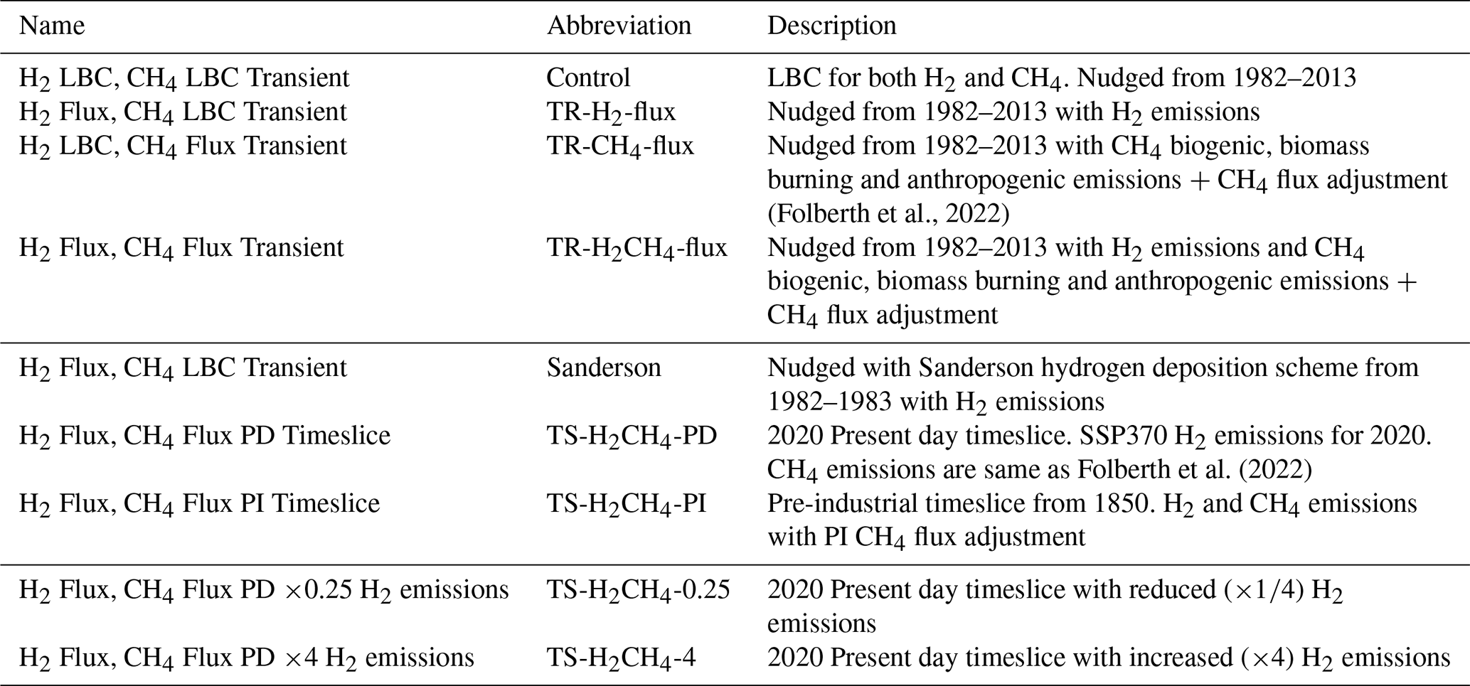
A total of four nudged simulations have been performed to compare the interactive fluxes; a control, two runs with either H₂ flux or CH₄ flux turned on, and one with both fluxes on. Table 1 shows a full list of the simulations run and a description of each. In addition to the four simulations, a fifth simulation using the hydrogen deposition scheme from Sanderson et al. (2003) with fixed methane LBC was run (named Sanderson in Table 1) to compare to another deposition scheme. The Sanderson scheme was only run for one year as there is only very limited interannual variability in the forcing soil temperature and soil moisture data from the land surface model, JULES (Pinnington et al., 2018). In addition to the nudged simulations, four timeslices were also performed including two scaled H₂ emission simulations. A timeslice experiment involves running the model with fixed sea surface temperatures, sea ice, and all other boundary conditions for a given year. One is under pre-industrial (PI) conditions (year 1850), while the other is present day conditions (year 2020). Timeslices for present day (TS-H₂CH₄-PD) and pre-industrial (TS-H₂CH₄-PI) with both interactive hydrogen and CH₄ are spun up for 30 years, with the former using CH₄ and H₂ (derived from CO) emissions from the Coupled Model Intercomparison Phase 6 project, using the Shared Socioeconomic Pathway 3 with a radiative forcing of 7.0 W m⁻² at the end of the 21st century i.e., SSP3-7.0 (Rao et al., 2017; Riahi et al., 2017) (see Sect. 2.2 for the calculation of H₂ emissions). Data are analysed over a 5-year period after the initial 25 year spin up, to allow for methane to reach a suitable steady state after 2.5 methane lifetimes.

While the LBC and interactive simulations offer a step by step response with and without interactive H₂ and CH₄ in a nudged scenario, these simulations are not directly comparable due to the differences in treatment of CH₄ and H₂ at the surface. In order to make an equal comparison, two additional timeslice simulations were run over the year 2020. The TS-H₂CH₄-PD run is used as a control, while in the other two simulations all H₂ emissions are continuously multiplied by $\mathrm{1}/\mathrm{4}$ (TS-H₂CH₄-0.25) and 4 (TS-H₂CH₄-4). These simulations are run for ten years to assess the response of CH₄ to different levels of H₂. The same starting conditions are used as the TS-H₂CH₄-PD simulation after the spin up period. Table 1 summarises these simulations.

2.2 Hydrogen Emissions

For the sources and quantities of primary hydrogen input to the model, we follow the method of Paulot et al. (2021). Hydrogen is released into the atmosphere from biomass burning and anthropogenic fossil fuel combustion. In addition, natural hydrogen sources associated with marine and terrestrial nitrogen fixation are also included. A summary of the emissions used for the nudged simulations is shown in Fig. A2.

As in Paulot et al. (2021), we use carbon monoxide (CO) emissions as a proxy for the evolution of hydrogen emissions trend. To obtain the amount of hydrogen emitted at any given time, we scale the corresponding CO emissions using a source specific ratio. The ratio of CO:H₂ for anthropogenic and biomass burning is derived from the period 1995–2014, where we have a known estimate of hydrogen emission (Table 1; Paulot et al., 2021) and can calculate the average CO emission over that time from emissions data.

The CO emissions used for the historical proxy are those created for UKESM1.0 for CMIP6 and detailed in Sellar et al. (2020). For anthropogenic and biomass burning emissions we use a historical timeseries (1850–2014). Anthropogenic emissions are taken from the Community Emissions Data System (CEDS-2017-05-18; Hoesly et al., 2018). For biomass burning we use those recommended for CMIP6 emissions (van Marle et al., 2017).

A seasonally varying climatology is used for natural emissions. Oceanic emissions use a monthly varying annual cycle for the year 1990 from the POET (Granier et al., 2005) inventory and apply it repeatedly. Terrestrial biosphere emissions are taken from the MACCity-MEGAN emissions inventory (Sindelarova et al., 2014), and a monthly varying annual cycle is taken from a mean of the years 2001–2010. All H₂ emissions are regridded from their native horizontal resolution to the N96 model grid (1.875°×1.25° longitude–latitude, approximately 135 km resolution) conserving mass. The resultant hydrogen emission for anthropogenic and biomass burning sources follow the spatial pattern of the equivalent CO source, but with values rescaled to give the global emission total appropriate for hydrogen. Scalings for oceanic and terrestrial H₂ emissions were set as 6 and 3 Tg respectively with the spatial distribution following that of CO as in Paulot et al. (2021). The hydrogen emissions are in agreement with Paulot et al. (2021) as shown in Fig. A2.

The year-2020 anthropogenic and biomass burning hydrogen emissions use the same source specific ratios of CO:H₂ as described above, and have been applied to year-2020 CO emissions from CMIP6 SSP3-7.0 (Gidden et al., 2019). The total biomass burning and anthropogenic H₂ emissions accounted for 7.6 and 14.9 Tg yr⁻¹ respectively. The TS-H₂CH₄-PI simulation used the same biomass burning hydrogen emissions as calculated for the nudged simulations, which extend back to 1850 and contributed 13.1 Tg yr⁻¹. The monthly varying climatologies for natural oceanic and terrestrial biosphere hydrogen emissions are invariant in time and, thus, are as described above.

2.3 CH₄ Flux Adjustment

Methane emissions used in the CH₄ flux experiments include biomass burning, anthropogenic, and biogenic emissions (Fig. A1). Biogenic wetland emissions and soil uptake are calculated interactively within the model, whereas all other emissions are prescribed (Hoesly et al., 2018; Fung et al., 1991). To reconcile simulated global mean surface methane concentrations with observations, a residual methane surface exchange flux, or flux adjustment, is applied in all simulations, following Folberth et al. (2022). This flux represents the net “missing” sources or sinks required in the emissions-driven configuration of UKESM to capture global methane observations. Separate flux adjustments are used for the pre-industrial (TS-H₂CH₄-PI) and present-day (TS-H₂CH₄-PD) timeslice simulations, as well as for the nudged simulations (TR-CH₄-flux and TR-H₂CH₄-flux). The PI and PD adjustments are taken directly from Folberth et al. (2022), with magnitudes of 5 and 48 Tg yr⁻¹ respectively. In the nudged simulations, a larger adjustment is required than in the PD timeslice because interactive wetland emissions are lower (135 versus 190 Tg yr⁻¹ in the PD simulation). This reduction in wetland emissions is consistent with a smaller global wetland fraction in the nudged configuration (0.0321) compared with the PD timeslice simulation (0.0358, an 11 % increase). To compensate for the reduced wetland source, as well as for differences in the chemical methane lifetime, the flux adjustment from the PD simulation was scaled by 3.5 in the nudged simulations to enable the model to capture the growth in surface global mean methane during the 1980s. Note that the flux adjustment is static across all years.

2.4 H₂ Soil Deposition Scheme

The model uses a two-layer hydrogen soil uptake scheme to calculate soil resistance (rc) based on the work by Ehhalt and Rohrer (2013) and Paulot et al. (2021), and used in Brown et al. (2025). The first layer represents the diffusion of hydrogen through the top layer of soil, while the second layer represents the loss from the microbial uptake of hydrogen. Two soil types, sand and loam, are included in the diffusion and microbial uptake parameterisation. The sand fraction of each gridbox is used to classify the soil type, with the remaining fractions (loam and clay) classified as loam. This is likely to lead to a slight overestimate in soil uptake in areas of high clay content, as hydrogen uptake in clays is known to be lower than loam (Bertagni et al., 2021; Cowan et al., 2025). The scheme also has a tuning parameter, α, which was scaled to the tropospheric hydrogen global burden of approximately 155 Tg to be in line results from Ehhalt and Rohrer (2009). Full details of the deposition scheme are given in Appendix A.

Different hydrogen deposition schemes vary in the inclusion of other deposition resistances (e.g. Bertagni et al., 2021). In this model, aerodynamic (ra) and laminar (rb) resistances are incorporated (Marrero and Mason, 1972; Hicks et al., 1987). Including these resistances results in the global hydrogen deposition velocity to decrease by 0.007 cm s⁻¹ (average 17.6 % decrease). The averaged land deposition velocity with all resistances is 0.0314 cm s⁻¹, while with just the uptake resistance the deposition velocity is 0.0380 cm s⁻¹. Figure 1 shows the monthly, land-averaged hydrogen deposition velocity with (pink) and without (purple) the additional resistances averaged between 1982–2013. The largest changes due to aerodynamic and laminar resistances occur over South America and Africa (excluding the desert), where deposition velocities can have a temporally averaged maximum difference up to 0.14 cm s⁻¹.

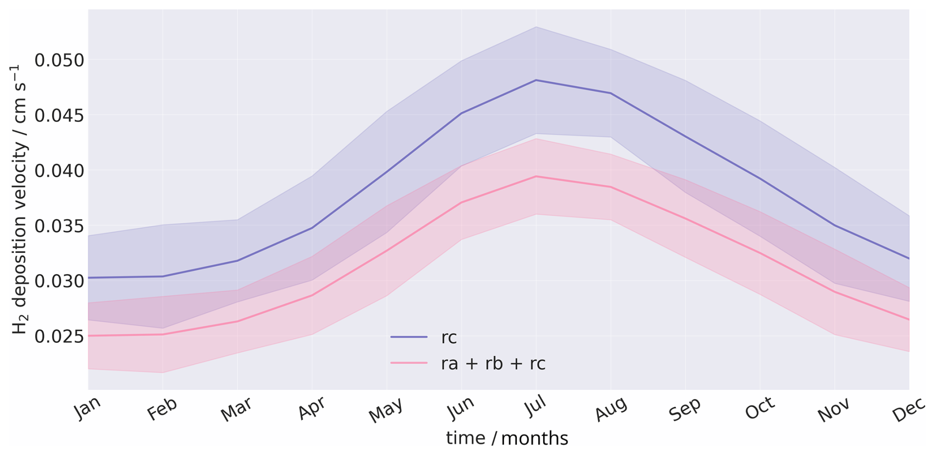
Figure 1 Monthly, land averaged hydrogen deposition velocity for simulation TR-H₂-flux (H₂ Flux; CH₄ LBC) between 1982–2013 with all resistances (pink) and with only hydrogen deposition velocity (purple). Shaded areas indicate two standard deviations.

An offline version of this model used in Brown et al. (2025) implemented a lower limit for uptake occurring in deserts, and a soil moisture cap for areas with a high soil moisture content (SMC). Both of these features are used in this model. If the volumetric SMC falls below a set of thresholds, the values for f_s(Θ_a) or f_l(Θ_a), which govern the microbial uptake, are set to one third of the minimum values under those temperature and soil porosity conditions, reflective of the findings in Jordaan et al. (2020) (see Appendix A, Eqs. A9 and A12 for more detail). For desert environments where the volumetric SMC is often below the threshold, this prevents the hydrogen deposition from immediately being set to zero, and allowing for uptake to occur in desert environments.

At locations of high volumetric SMC relative to the soil porosity, hydrogen cannot diffuse through the top layer of soil and hydrogen deposition is very low. In UKESM1.0, the ratio of volumetric SMC to total porosity ($\frac{\text{volumetric SMC}}{\text{soil porosity}}$) is very high at northern latitudes with an annual average of >0.85. Observed volumetric SMC during summer in these regions is between 0.15–0.3 m³ m⁻³ (Dorigo et al., 2023), which, if using the soil porosity from UKESM1.0, produces $\frac{\text{volumetric SMC}}{\text{soil porosity}}\le \mathrm{60}$ %. This high ratio from UKESM1.0 is likely to be inaccurate due to the soil porosity not capturing the large coverage of peatland at these latitudes. Soil porosity is calculated using sand fraction and does not take into account soils such as peatlands, which have been found to have a high hydrogen uptake (Simmonds et al., 2011). In order to compensate for the high volumetric SMC to porosity ratio, the $\frac{\text{volumetric SMC}}{\text{soil porosity}}$ ratio in the hydrogen deposition scheme is capped at 70 %. The volumetric SMC is adjusted so the maximum ratio does not exceed this value.

3 Evaluation of H₂ Deposition

The hydrogen deposition previously implemented in UKESM1.0 used the scheme from Sanderson et al. (2003). This deposition uptake was based on soil land type and scaled the deposition linearly or quadratically with soil moisture depending on the land type. While this produces global deposition velocities in line with other global hydrogen deposition values (see Sand et al., 2023), it does not include uptake in deserts, and is limited by requiring the land-use type within a grid cell. The scheme adapted from Paulot et al. (2021), which is used in this work allows for an interactive hydrogen flux, is dependent on soil properties and thus can be used for scenarios in which the land type is not known or prescribed (e.g. pre-industrial conditions, future climate simulations).

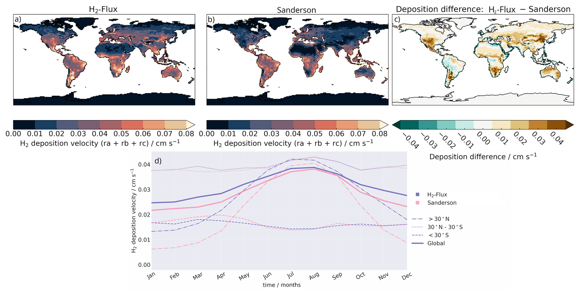
Figure 2 Annually averaged hydrogen deposition velocity in 1982 for (a) TR-H₂-flux using deposition scheme adapted from Paulot et al. (2021), (b) Sanderson et al. (2003) deposition (H₂ Flux; CH₄ LBC), and (c) difference between the two schemes (a–b). (d) Land-averaged monthly mean hydrogen deposition velocities of (purple) TR-H₂-flux and (pink) Sanderson for 1982. Linestyles indicate 30° latitude bands into which data have been divided, with the thickest line showing the global-averaged deposition.

Figure 2 shows the comparison of hydrogen deposition velocities between the scheme adapted from Paulot et al. (2021) and the scheme from Sanderson et al. (2003). Both simulations have the same model configuration, using the same hydrogen emissions, “nudged” winds and air temperature from ERA5 data as per Telford et al. (2008). The TR-H₂-flux simulation has a greater hydrogen deposition in the northern hemisphere (>30° N) than in the Sanderson scheme, with deposition increase of 0.02–0.04 cm s⁻¹ in North America and Central Asia (Fig. 2c). This is also seen by the dash-dotted lines in Fig. 2d, which show the land-average deposition velocity above 30° N; the TR-H₂-flux simulation (purple) is between 0.002–0.005 cm s⁻¹ greater than the Sanderson et al. (2003) (pink) simulation. Both simulations share a seasonal cycle which is dominant in northern latitudes, with the Sanderson et al. (2003) simulation having a larger amplitude in seasonality. The TR-H₂-flux simulation has an overall higher deposition velocity (9.2 % higher) throughout the year than that of the Sanderson et al. (2003) scheme (thick solid lines in Fig. 2d), with an annual, land-averaged mean of 0.0312 cm s⁻¹ compared to 0.0285 cm s⁻¹ respectively. This is due to uptake occurring in the desert, as well as in the tropics and at high northern latitudes.

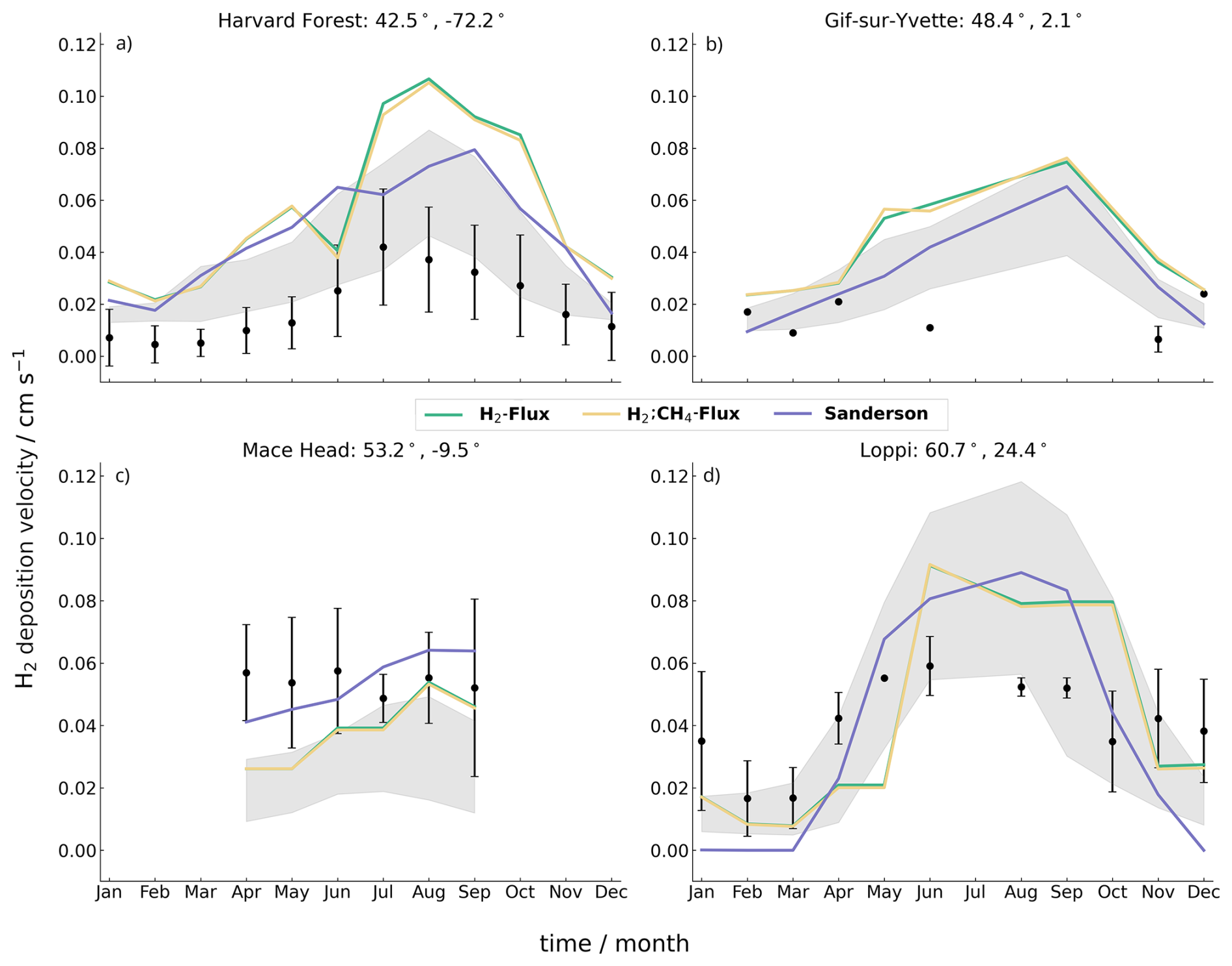
Figure 3 Monthly mean observed hydrogen deposition velocities averaged across years where possible (points) compared with (green) TR-H₂-flux, (yellow) TR-H₂CH₄-flux, and (purple) Sanderson simulated velocities for (a) Harvard Forest (2010–2012; Meredith et al., 2017), (b) Gif-sur-Yvette (2011; Belviso et al., 2013), (c) Mace Head (1995–2008; Simmonds et al., 2011), and (d) Loppi (2004–2006; Lallo et al., 2008). Error bars show one standard deviation across years. Shaded areas show the range of deposition velocities from CMIP6 model inputs calculated in Brown et al. (2025).

Figure 3 shows simulated hydrogen deposition against observations at four different sites, all of which are located in the northern hemisphere. The land types of (a) Harvard and (d) Loppi are deciduous and boreal forests respectively, while (b) Gif-sur-Yvette and (c) Mace Head are grassland/agriculture and peatbogs respectively. The soil types of all sites are different, with Harvard Forest as sandy loam, Loppi as mineral and peat soils, and Mace Head as peatland (Gif-sur-Yvette not given). TR-H₂-flux and TR-H₂CH₄-flux simulations were compared against the observations. Both simulations produce very similar hydrogen velocities, globally and at all individual sites, which is expected as there is little atmospheric influence on the hydrogen deposition velocities. Shaded areas show the range of deposition velocities from CMIP6 model inputs calculated in Brown et al. (2025), while the purple line shows the deposition velocities from the Sanderson simulation. Compared to observations and other simulations, the TR-H₂-flux and TR-H₂CH₄-flux simulations tend to overestimate deposition velocity, with the exception of Mace Head.

At Mace Head, the hydrogen deposition velocities are underpredicted in April–May and are outside of the range of observed deposition velocities, although within the standard deviation of observations for the remaining months (June to October). Gif-sur-Yvette lacks observations during the summer months and thus there is no defined peak to which the simulations can be compared directly. However, between November–April, deposition velocities are within 0.005 cm s⁻¹ of the observations. In both Harvard Forest (a) and Loppi (b), deposition is overpredicted by 0.02–0.04 cm s⁻¹, with the largest discrepancy for both sites occurring in the summer months. The CMIP6 range also overpredicts deposition at these sites, although not to the same extent (up to 0.02 cm s⁻¹). Overestimates in the TR-H₂-flux and TR-H₂CH₄-flux deposition velocities correspond with underestimates in hydrogen mixing ratios in the northern hemisphere.

4 Results

4.1 Comparison to Atmospheric Observations

In order to evaluate the skill of the model, the hydrogen and methane outputs are first compared to multiple years of observations (Prinn et al., 2018). Figure 4 compares surface observations of (a) hydrogen and (b) methane with the simulated TR-H₂CH₄-flux values. Observations at two stations are shown; Mace Head in the northern hemisphere (MHD; green) and Cape Grim in the southern hemisphere (CGO; orange). These sites were chosen as they had the longest continuous H₂ record available in the northern and southern Hemispheres, as well as their locations’ suitability for monitoring baseline atmospheric conditions. The latitude and longitude of simulated values were matched by nearest neighbour to the closest location of the station sites. The simulated hydrogen mixing ratios for Mace Head are in good agreement with the observations. There is a small overprediction up to 15 ppbv between 1994–2000, but after the year 2000 the simulated hydrogen is in line with the observations. The simulated hydrogen captures the trend post 2003 at Cape Grim, but does not do as well prior to this. Furthermore at Cape Grim, hydrogen is consistently overpredicted during the southern summer, where hydrogen can be up to 35 ppbv greater than observed values. The minimum hydrogen mixing ratios are captured during southern winter, suggesting that the seasonal cycle of hydrogen is too strong in the model. This may be due to too extreme changes in soil moisture between the winter and summer months (Pinnington et al., 2018).

Simulated methane is slightly underpredicted when compared with observations from Cape Grim. This is seen in Fig. 4b from 1995 onwards, where there is a 50 ppbv low bias with respect to observations in the model. Similarly, in the northern hemisphere, methane at Mace Head is generally in good agreement with observations from 1997 onwards (50 ppbv excess). Between 1992–1997, there is a larger difference, which reaches up to 100 ppbv. The model captures the overall trend and seasonal cycle of observations.

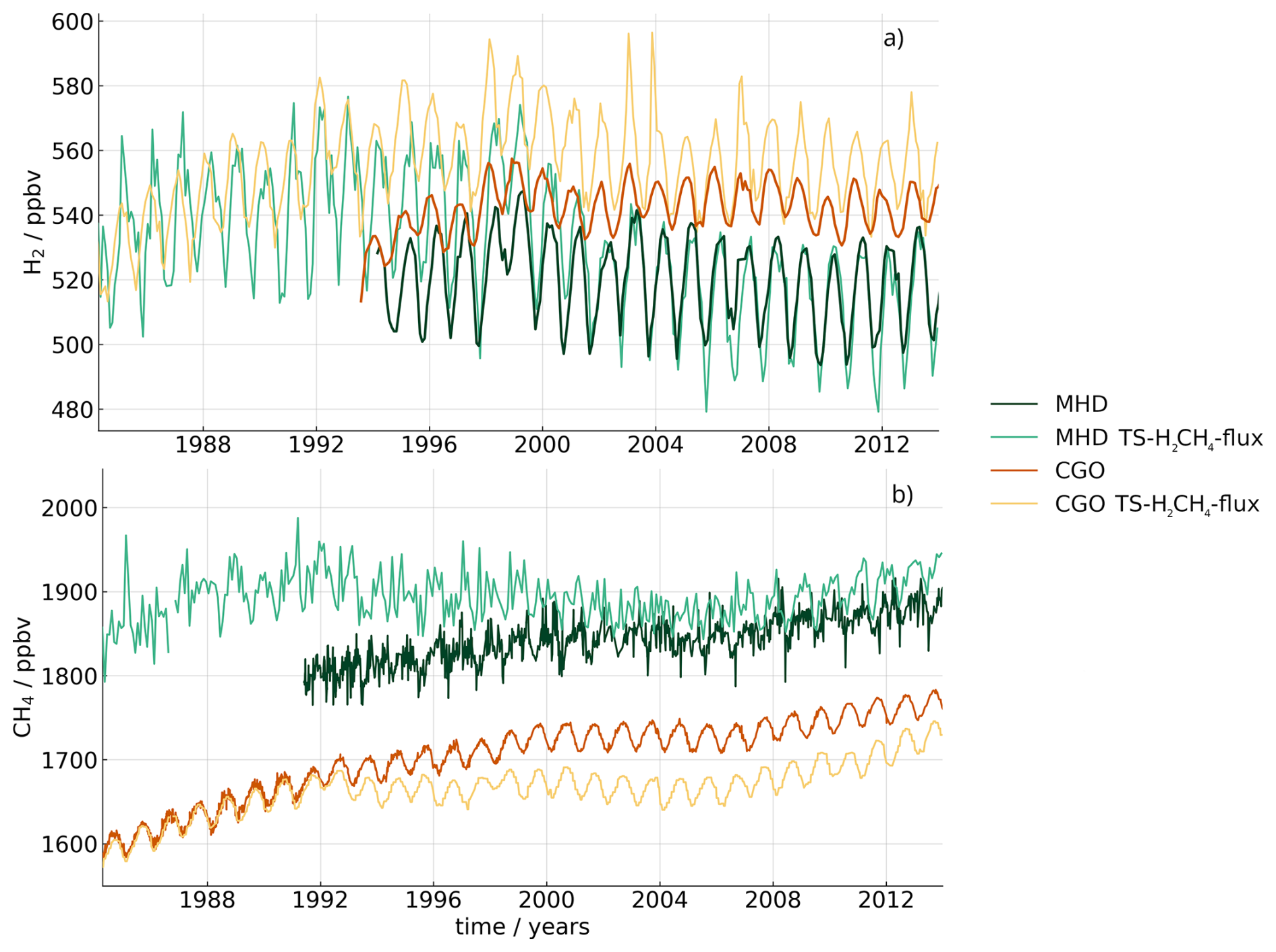
Figure 4 Time series of Mace Head for (MHD: dark green) observations and (light green) TR-H₂CH₄-flux simulation, and Cape Grim (CGO: orange) observations and (yellow) TR-H₂CH₄-flux for (a) hydrogen (observations: 1994–2013) and (b) methane (observations: 1985–2013).

Further to these two sites, the simulated hydrogen is compared to observations at all NOAA stations (Pétron et al., 2024). Observed data have been monthly averaged to match the same time resolution as the modelled data. Simulated hydrogen has been matched to observations by nearest latitude and longitude, and time up to the year 2013. Hydrogen observations after the year 2013 are discarded as simulations were run for the historical time period used in CMIP6, where there was availability of historical emissions. Figure 5a summarises the variance via normalised standard deviation (NSD) and correlation between simulated and observed hydrogen, while Fig. 5b shows the average surface hydrogen mixing ratios for the TR-H₂CH₄-flux simulation (on map) and observation sites (points).

In Fig. 5a, sites in the northern hemisphere are blue, while southern sites are in red. Table A1 gives the numerical key for each site. Values close to the point marked “REF” (which is 1) show that the standard deviation of the model and observation site are very similar, implying they have a similar variation. The correlation conducted uses a standard Pearson's correlation test, and only stations with more than 20 datapoints pre-2014 were used in the experiment. Values with a higher correlation indicate that the seasonal trend of observed hydrogen is captured.

In Fig. 5a, a greater proportion of southern sites (dark red) have a high correlation (>0.8), suggesting they capture the seasonal trend. The NSD tends to be greater than 1, implying that there is too much variation in the modelled data and that, while the seasonal cycle is captured well, the amplitude in the simulated data is larger than the observations. For northern sites, there is a spread of how well the simulated hydrogen captures the variation from observations. At sites where the model has too much variation (NSD >1), the correlation tends to be greater (between 0.65–0.95), similar to the southern sites. This is similar to the findings from the deposition comparison at Harvard Forest and Loppi (Fig. 3a and b), where there is too much deposition occurring during the summer.

Values with an NSD <1 tend to have a lower correlation, suggesting the model does not capture the observed variation at these sites. Overall, most sites have an NSD around 1 and a correlation between 0.6–0.9, indicating the simulation captures the seasonal spread and cycle.

Figure 5b shows the simulated surface hydrogen mixing ratio averaged from 2008–2013 with the averaged hydrogen mixing ratio from all sites given as points. The hydrogen mixing ratio is high (>580 ppbv) in Africa between 5° N–25° S due to biomass burning and natural emissions, despite the larger deposition velocity over that region. The simulated data captures the hydrogen mixing ratios within 20 ppbv at nearly all observation sites. The exception to this is the very high (>620 ppbv) hydrogen mixing ratio over China and India, which results from the combination of anthropogenic emissions and orography in the model which is known to lead to an overestimation in emissions (Hayman et al., 2014). Overall, the model slightly overpredicts hydrogen in the southern hemisphere by an average of 13.2 ppbv, while in the northern hemisphere there is a small averaged underprediction of 2.1 ppbv. In general, the model is able to capture the average magnitude of hydrogen mixing ratios at most sites, and replicates similar correlations and variations to those in the observations.

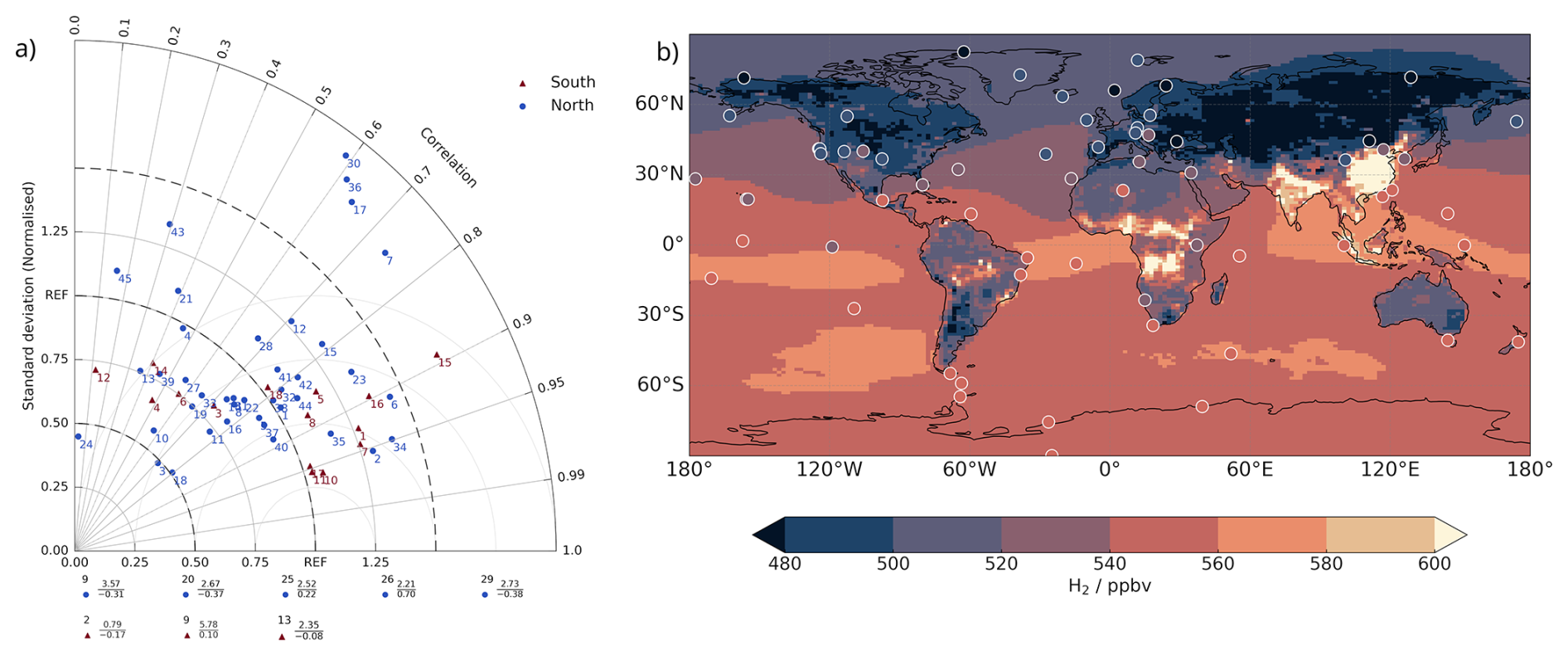
Figure 5 (a) Taylor diagram showing Pearson's correlation and the standard deviation of modelled data (TR-H₂CH₄-flux) normalised to observations for all different sites. Red triangles show sites in the southern hemisphere, while blue triangles show sites in the northern hemisphere. Anomalies with either too high a NSD or negative correlation are excluded from the diagram and written below with the format $\frac{\text{normalised standard deviation}}{\text{correlation}}$. Labels correspond to sites as given in Table A1. (b) Map of averaged surface hydrogen mixing ratio from TR-H₂CH₄-flux run overlaid with averaged hydrogen mixing ratios from each NOAA site. All simulated data are averaged between 2008–2013.

4.2 Impact of Fluxes on Atmospheric Composition

Ozone and OH are both trace gases sensitive to chemical fluctuations in the atmosphere, due to their high reactivity. Global methane mixing ratios are relatively unchanged with interactive CH₄, and there is a small increase in the global hydrogen mixing ratio (from 500 ppbv in the control to 550 ppbv in the TR-H₂-flux simulation for 2008–2013) when adding in interactive H₂ (Warwick et al., 2023). Thus, as expected when adding in both the hydrogen and methane flux, there is minimal impact on tropospheric ozone or OH, as shown in Fig. 6. There is up to a 40 ppbv change in ozone between the control and TR-H₂CH₄-flux simulation, which corresponds to a 4 % decrease. Similarly, there is less than 5×10⁴ molecules cm⁻³ increase in OH density in the troposphere (3 % increase), and a decrease of 4×10⁴ molecules cm⁻³ in the stratosphere (5 % decrease).

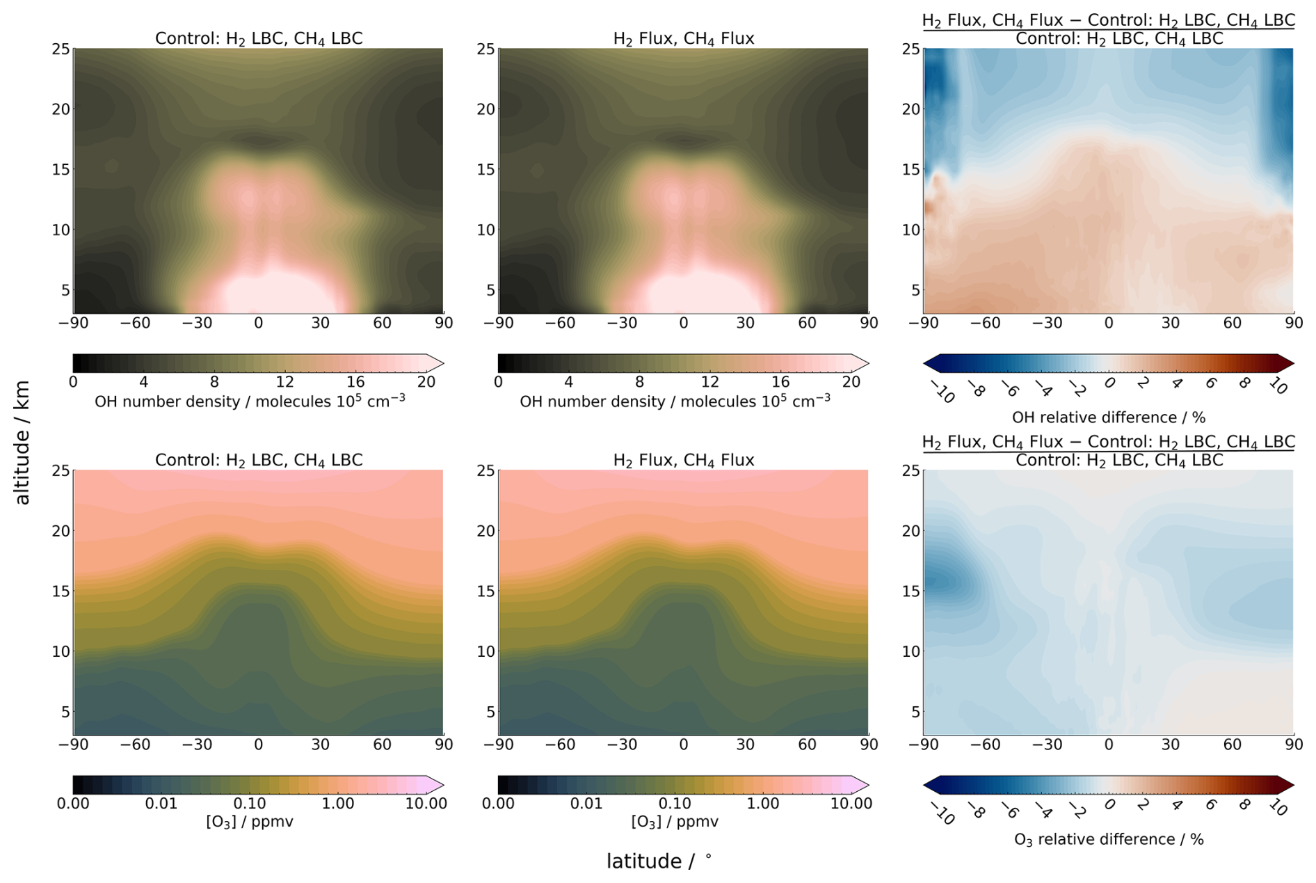
Figure 6 Zonally averaged (top) OH concentration and (bottom) ozone mixing ratio for the (left) control simulation, (middle) TR-H₂CH₄-flux simulation, and (right) the relative difference between the two ((TR-H₂CH₄-flux − Control)$/$Control) averaged between 2008–2013. Red (blue) shows an increase (decrease) from the control.

The global surface average of hydrogen and methane is shown in Fig. 7. In both the TR-H₂CH₄-flux and TR-H₂-flux simulations, global surface hydrogen equilibrates to 545 ppbv with an average ±12 ppbv seasonal cycle. In 1992 and 1998, there are sharp increases of hydrogen due to the increase of biomass burning in these years (Fig. A2), and, in 2002, hydrogen equilibrates to between 540–550 pbbv. The replacement of the fixed methane LBC to flux has little impact on hydrogen both globally averaged and across all latitudes (not shown). The control and TR-CH₄-flux simulations both use a fixed H₂ LBC of 500 ppbv, which is constant across all times of year and latitude.

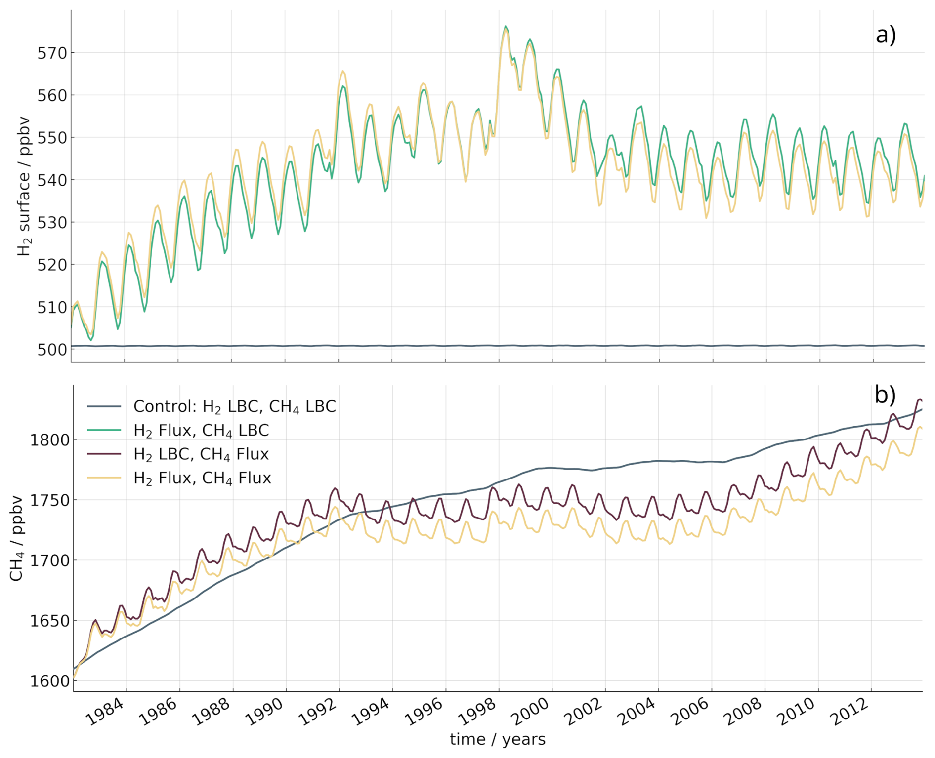
Figure 7 (a) Globally averaged surface hydrogen from the (grey) control, (green) TR-H₂-flux, and (yellow) TR-H₂CH₄-flux simulations from 1982 to 2013. Both the control and the TR-CH₄-flux simulation have hydrogen set to 500 ppbv at the surface. (b) Globally averaged surface methane from the (grey) control, (red) TR-CH₄-flux, and (yellow) TR-H₂CH₄-flux simulations.

Figure 7b shows the surface global methane from the (grey) control and with methane flux with (red) H₂ LBC and (yellow) hydrogen flux implemented. Between 1996–2012, the surface methane mixing ratio in both simulations is slightly below the control by up to 30 ppbv (∼1.7 % difference). The two simulations with methane flux are in good agreement with the fixed LBC values (the latter of which is based on observations). They capture both the trend pre-1992 and the levelling off of methane abundance between 1998–2007, as well as the increasing trend after 2007.

The global averaged surface methane mixing ratio decreases when the fixed H₂ LBC is replaced by H₂ flux; the global, surface average methane is approximately 20 ppbv lower from 1998 onwards. The decrease in methane in the TR-H₂CH₄-flux simulation occurs across all latitudes, with a greater decrease occurring in the northern hemisphere (not shown).

One explanation for this is due to the change in surface distribution for H₂ mixing ratio which impacts the OH reactivity. This is a result from the technical differences in simulations (e.g. interactive flux vs fixed LBC). Figure 8 shows the one over the rate coefficient of (top) H₂ chemical loss and (bottom) CH₄ loss via OH ($\frac{\mathrm{1}}{k\left[\mathrm{OH}\right]}$), which shows the OH reactivity of these reactions, and simultaneously the respective chemical lifetimes of H₂ and CH₄. Blue (red) indicates a decrease (increase) in lifetimes when H₂ flux is included, relative to the simulation with fixed H₂ LBC.

The surface hydrogen mixing ratio in the southern hemisphere increases up to 580 ppbv (as seen in Fig. 5b), while decreasing in the northern hemisphere down to <480 ppbv. The shift in hydrogen distribution causes a change in OH reactivity. In the southern hemisphere, the CH₄ lifetime via OH increases by up to 0.4 %, which can be seen at the surface between 30–60° S (red) in bottom right panel Fig. 8. In the northern hemisphere, the CH₄ lifetime via OH decreases by ∼0.3 % (blue in top right panel of Fig. 8). This is a result of the reduction in H₂ mixing ratio at the surface in the northern hemisphere, which is directly due to the stronger soil uptake over northern American and Siberia.

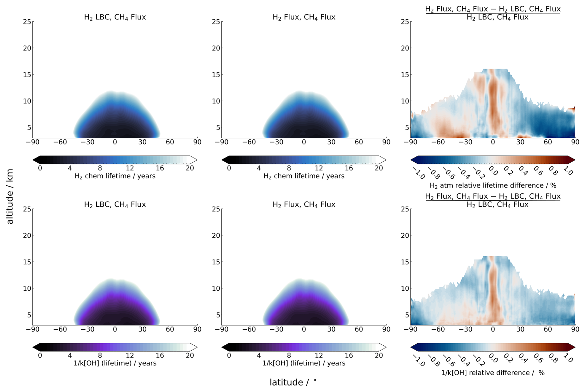
Figure 8 Zonally averaged (top) H₂ chemical loss lifetime and (bottom) CH₄ lifetime via OH for (left) TR-CH₄-flux simulation, (middle) TR-H₂CH₄-flux simulation, and (right) relative difference between the two (CH₄-flux − TR-H₂CH₄-flux) averaged between 2008–2013. Red (blue) shows an increase (decrease) in lifetimes from the TR-CH₄-flux. The stratosphere has been masked out to reduce noise.

The different surface set ups (fixed LBC versus interactive flux) are not a fair direct comparison of the response of CH₄ to H₂. To examine the impact of a change in H₂ on CH₄ without the added complication of the fixed LBCs, three additional timeslice simulations were analysed; a control (TS-H₂CH₄-PD), one with reduced H₂ emissions (75 % reduction; TS-H₂CH₄-0.25), and another with increased H₂ emissions (300 % increase; TS-H₂CH₄-4). Figure 9 summarises the globally averaged surface mixing ratios of (a) H₂ and (b) CH₄ for 10 years. Figure 9c shows the monthly, globally average surface difference between the control and the altered emissions simulations (control – altered emissions). The black line shows there is no change from the control. The TS-H₂CH₄-4 simulation shows that CH₄ increases as H₂ increases. In particular, there is a non-linear relationship between the two species in the ×4 H₂ emission simulation. This is likely due to H₂ reaching steady state much quicker than CH₄ as its lifetime is shorter (2 years compared to 10 years), while CH₄ continues to increase in response to H₂ (Fig. 9c).

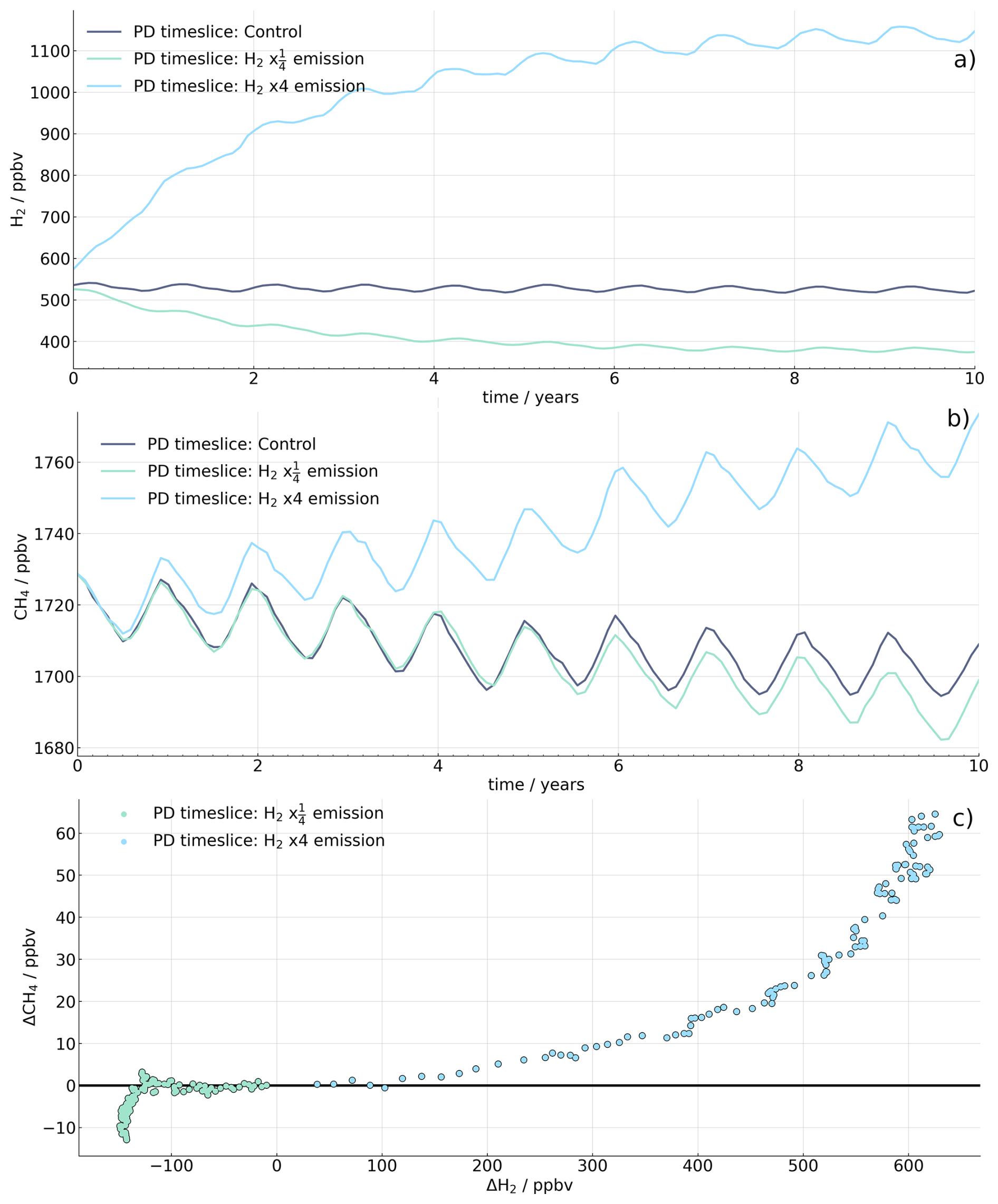
Figure 9 Global monthly averaged (a) H₂ and (b) CH₄ surface mixing ratios of the (dark blue) control, (green) $\mathrm{1}/\mathrm{4}$ H₂ emissions, and (light blue). (c) Difference between the control PD timeslice and the perturbed H₂ emissions simulations (perturbed emissions – control). Black line indicates no difference from the control. Timeslices are for 2020.

4.3 H₂ and CH₄ Budget

Both the hydrogen and methane lifetimes calculated in this work include the burden of the whole atmosphere. The hydrogen lifetimes and burdens are summarised in Table 2, while the methane lifetime for the nudged simulations is summarised in Table 3. Budget for the PI and PD timeslices are discussed in Sect. 4.4.

Hydrogen lifetime is similar between all simulations, ranging between 2.41–2.48 years. The soil lifetime remains constant, while the lifetime from chemical loss reactions fluctuates between 7.01–7.73 years. Soil lifetime is expected to produce similar values between all runs, as the deposition is calculated through soil properties and is independent of hydrogen. In Sand et al. (2023), soil lifetime was estimated from prescribed H₂ LBC values and both the soil and total model-averaged hydrogen lifetimes are similar to values in this work.

Sand et al. (2023)Surawski et al. (2026)Ehhalt and Rohrer (2009)

Table 2 Hydrogen lifetime and budget of different simulations. Present day and pre-industrial timeslices are averaged over the last 5 years, nudged runs are averaged between 2008–2013. Lifetime is given in years. Burden is in Tg, while chemical production, chemical loss, and emissions are given in Tg yr⁻¹.

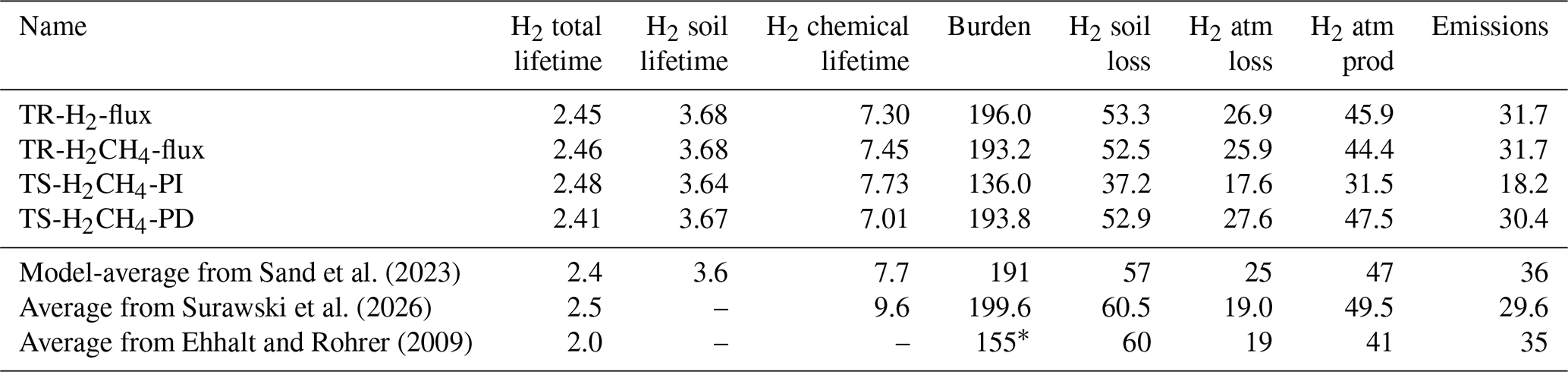
^* This is tropospheric H₂ burden.

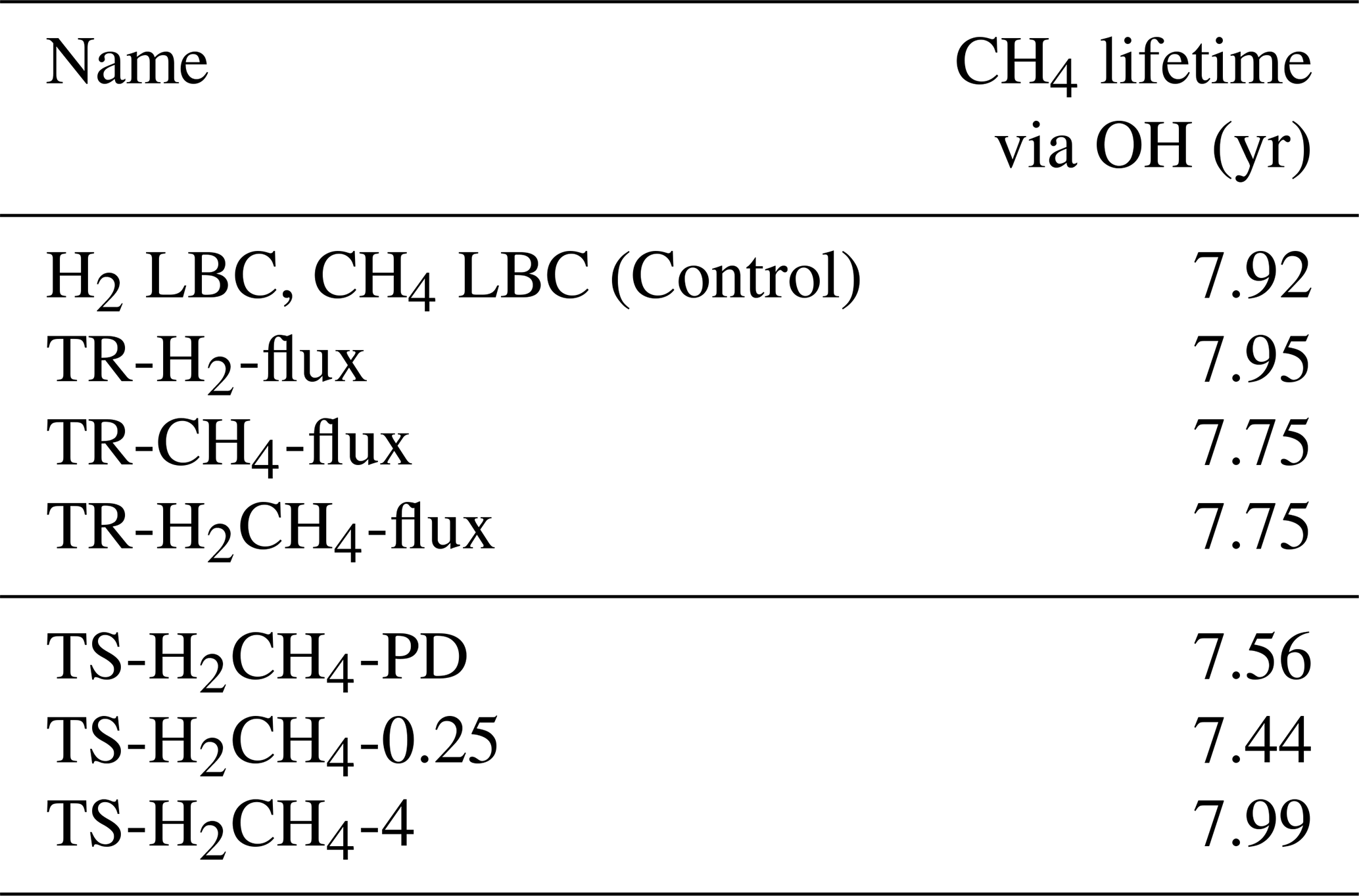
Methane lifetime decreases when including methane flux (0.167 years; 2.1 %), due to the slightly lower abundance of methane than the LBC condition. This will reduce the feedback on CH₄, which is consistent with the findings from Folberth et al. (2022). The changes between methane lifetime via OH loss are minimal, as shown in Table 3. When implementing H₂ flux into the ESM with a fixed CH₄ LBC, there is a small increase in methane lifetime. This is in agreement with the work conducted in Warwick et al. (2023), who ran a series of experiments with increasing H₂ LBC to assess the impact on methane. They found that when hydrogen abundance increased, the methane lifetime via OH reaction increased. When comparing the CH₄ flux simulations with and without H₂ flux, however, there is no difference in methane lifetime (both are 7.75 years to 2 decimal places). Further to this, the global surface methane mixing ratio decreases by 25 ppbv. This difference in global surface methane mixing ratio is due to the spatial distribution of H₂ from the different methodologies (e.g. interactive flux and fixed LBC), and is therefore difficult to directly compare against. Table 3 also shows the CH₄ lifetime via OH loss for the present day timeslices with adjusted H₂ emissions. The TS-H₂CH₄-0.25 simulation which has lower H₂ emissions is 0.12 years lower than the present day control, while the TS-H₂CH₄-4 with increased H₂ emissions has an increased CH₄ lifetime of 0.43 years. Given that these differences are larger than in the nudged simulations and are not obscured by different methodologies (all present day timeslices have both H₂ and CH₄ interactive flux), the response of CH₄ to an increase in H₂ is in agreement with Warwick et al. (2023).

Table 3 Methane lifetime via OH loss in years from four nudged simulations (averaged over 5 years between 2008–2013) and three PD timeslices (averaged over the last 5 years of the 10 year simulation) to 3sf.

4.4 Pre-industrial and Present Day H₂

One application of the combined CH₄-H₂ emissions driven capability is to explore drivers of the combined CH₄-H₂ evolution over the industrial period. The links between the two species provide a new opportunity for joint constraints on uncertainty in the emissions and sinks of these two gases. The pre-industrial simulation run from 1850 (TS-H₂CH₄-PI) has a much lower hydrogen burden of 136.0 Tg than present day (PD) simulations due to having very low anthropogenic emissions. Despite this, the overall hydrogen lifetime is still in line with other present day simulations (2.48 years; Table 2).

Figure 10 shows the hemispherically-averaged surface hydrogen and methane mixing ratio from the (a) PI (TS-H₂CH₄-PI) and (b) PD simulation (TS-H₂CH₄-PD). The PI simulated surface methane mixing ratio (Fig. 10a) does not have a strong gradient between hemispheres. Using ice core data from Antarctica and Greenland, Etheridge et al. (1998) showed there was a 24 ppbv discrepancy between hemispheres in the 1850s; with southern hemisphere at 785 ppbv and northern hemisphere values at 809 ppbv. The TS-H₂CH₄-PI simulation has an annual average of 761 ppbv (SH) and 765 ppbv (NH). Both hemispheres have overlapping inter-annual variability (1 standard deviation), indicating there is no significant difference between hemispheres.

Hydrogen in the northern hemisphere has a strong seasonal cycle and ranges between 405 ppbv (March) to 360 ppbv (October) due to the strong deposition seasonality (as seen in Fig. 2). In the southern hemisphere, the surface mixing ratio remains consistent between 372–375 ppbv. The southern hemisphere hydrogen mixing ratios can be compared directly with hydrogen mixing ratios reconstructed from firn air from Antarctica (Patterson et al., 2021). Around 1850s, Patterson et al. (2021) found that hydrogen levels were 330±15 ppbv, which are slightly lower than the modelled mixing ratio from the TS-H₂CH₄-PI simulation. Firn air measurements for the northern hemisphere are only reconstructed back to 1950s, where the hydrogen mixing ratio was $\sim \mathrm{400}\pm \mathrm{25}$ ppbv (Patterson et al., 2023). The annually averaged TS-H₂CH₄-PI hydrogen mixing ratio in the northern hemisphere is in agreement with the reconstructed firn data from 1950s. It is likely, however, that the hydrogen mixing ratio was lower in the 1850s, similar to that seen in the southern hemisphere. Thus, the simulated hydrogen values are likely overestimated.

There is a shift in the seasonal cycle of hydrogen in the PI simulation compared to the present day (Fig. 10b; note the different axis for hydrogen mixing ratio for PI and PD). In the northern hemisphere, hydrogen concentration peaks around April–May in PD run, while in the PI simulation, hydrogen peaks earlier in the year (March). This is likely due to a smaller chemical source in the summer in the TS-H₂CH₄-PI simulation, where production only reaches up to 0.38 mol s⁻¹ compared to 0.57 mol s⁻¹ in the TS-H₂CH₄-PD simulation. The smaller chemical production results in a shift in the peak of surface H₂ mixing ratio to earlier in the year, relative to the present day. Further to this, there is a relative decrease in southern hemisphere emissions in the TS-H₂CH₄-PI simulation (due to reduced biomass burning) compared to the TS-H₂CH₄-PD simulation, resulting in a smaller difference in hydrogen mixing ratios between hemispheres when comparing between PI and PD scenarios (Fig. 10c). Overall, there is a lower seasonal amplitude in the southern hemisphere in the PI scenario due to a smaller seasonal amplitude in the hydrogen chemical production (PI: 0.06 mol s⁻¹ with PD: 0.26 mol s⁻¹), as well as there being no anthropogenic emissions in the PI scenario.

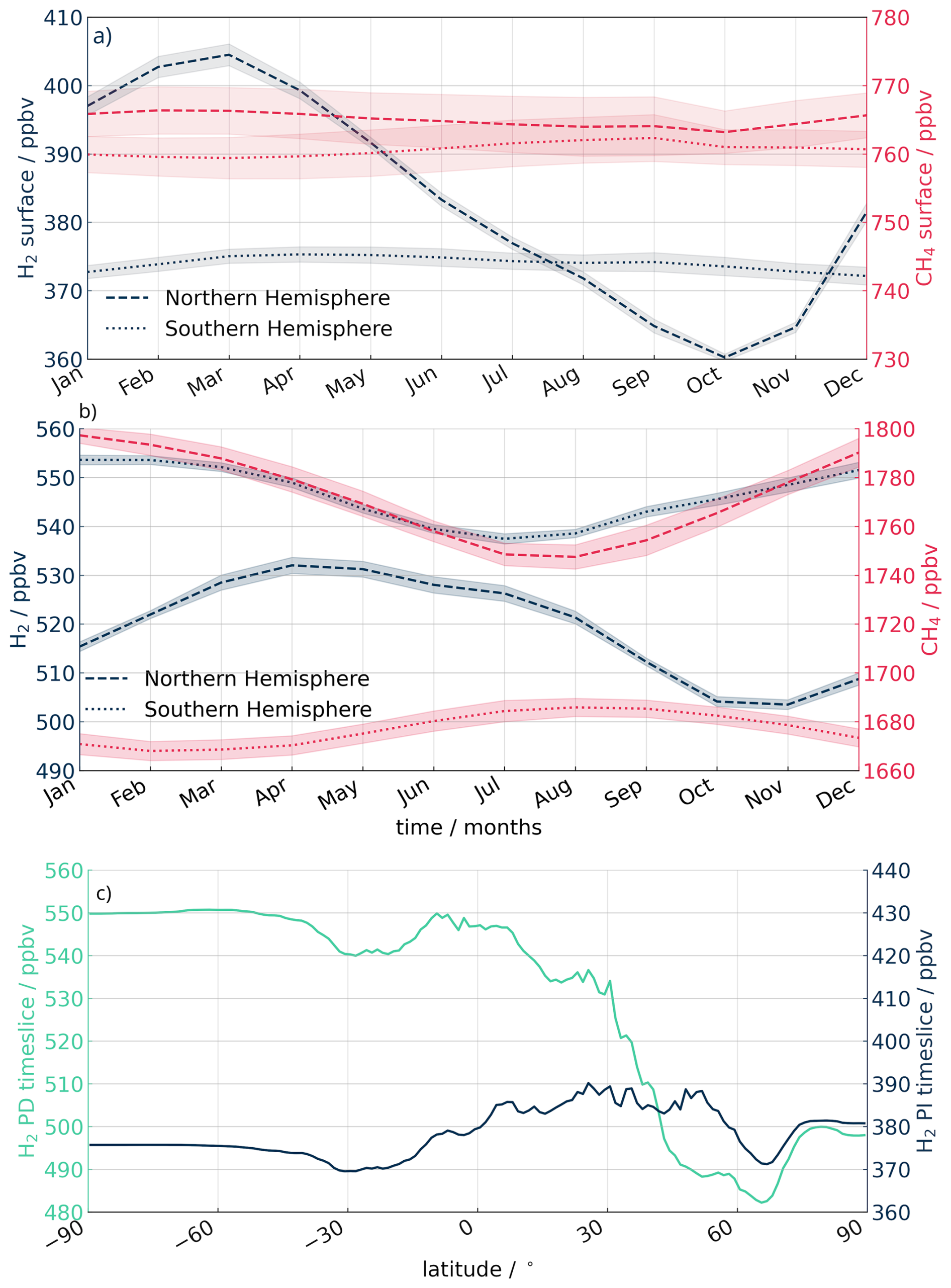
Figure 10 Five-year hemispherical averages of surface hydrogen (blue) and methane (red) mixing ratios for (a) 1850 (TS-H₂CH₄-PI simulation) and (b) 2020 (TS-H₂CH₄-PD simulation). Dashed lines show the northern hemisphere, while dotted lines show the southern. Shaded areas show one standard deviation calculated from the last five years of the simulation. (c) Zonally averaged surface hydrogen mixing ratio for (blue) PI and (green) PD simulations (averaged over give years).

5 Conclusions

Hydrogen and methane are closely coupled species in the atmosphere, with both tracers competing for OH as their main atmospheric destruction pathway. We have implemented a hydrogen soil sink scheme into an ESM, along with adding the methane flux from Folberth et al. (2022) to create a fully coupled H₂-CH₄ ESM. Implementing H₂ flux caused the global average surface hydrogen to equilibrate to 540−550 ppbv, which has been tuned via the soil sink (see Appendix A) to literature values of the tropospheric hydrogen burden (Ehhalt and Rohrer, 2009). The model was able to capture the hydrogen seasonal cycle, which is dominant in the northern hemisphere and is primarily driven by the soil sink.

The inclusion of both H₂ flux and CH₄ flux had a minimal impact on the overall OH concentration and ozone mixing ratio in the model, and there was little change in hydrogen mixing ratios when CH₄ LBC was replaced with CH₄ flux. Hydrogen and methane mixing ratios were compared against observations at a northern site (Mace Head) and a southern site (Cape Grim). In general, both species were found to capture the magnitude and the seasonal cycle of the observations when H₂ flux and CH₄ flux were on.

When implementing H₂ flux into the ESM with CH₄ flux, we found methane lifetime remained the same and the overall global surface mixing ratio of methane decreased. This decrease is due to the change in the spatial distribution of hydrogen at the surface when switching from fixed H₂ LBC to H₂ flux, the former of which has no spatial variability. With the replacement of H₂ LBC to H₂ flux, the overall global surface hydrogen mixing ratio increased. However, the hydrogen mixing ratio decreased in the northern hemisphere as a result of the soil sink, which led to a decrease in the CH₄ lifetime via OH, and a lower global surface CH₄ mixing ratio.

When H₂ flux and CH₄ flux are included, the ESM is able to simulate PI conditions which are within a similar order of magnitude as concentrations found in firn measurements. The seasonal cycle of hydrogen in the PI simulation shifted and peaked earlier in the year, and the gradient between northern and southern mixing ratio was much smaller, with the hydrogen mixing ratio in the north exceeding that of the south between December–July.

These initial experiments show the potential of a fully interactive hydrogen and methane model. Coupling H₂ flux and CH₄ flux into the ESM allowed the impact of hydrogen on methane to be analysed, and was found to cause a small global decrease in methane. A further set of experiments perturbing H₂ emissions in a present day timeslice showed a similar response as Warwick et al. (2023), where an increase in H₂ results in an increase of CH₄. The small decrease in CH₄ in the nudged simulations when replacing a fixed H₂ LBC with a H₂ flux is, therefore, due to comparing different methodologies of surface interactions (interactive flux versus fixed boundary layer). This behaviour highlights the importance of having a fully coupled hydrogen and methane model to further understand their interaction and, ultimately, provide a better estimate of their GWP in present day and future scenarios.

Appendix A: Hydrogen Deposition Scheme

These equations are adapted from Ehhalt and Rohrer (2013) and Paulot et al. (2021). The equation for hydrogen deposition velocity, v_d(H₂) (also known as $\frac{\mathrm{1}}{\mathrm{rc}}$), is given by,

$$\begin{array}{}\text{(A1)}& v_{\mathrm{d}}\left({\mathrm{H}}_{\mathrm{2}}\right)={\displaystyle \frac{\mathrm{1}}{\frac{\mathit{\delta }}{D_{\mathrm{s}}}+\frac{{\mathit{\delta }}_{\mathrm{snow}}}{D_{\mathrm{snow}}}+\frac{\mathrm{1}}{\sqrt{D_{\mathrm{s}}{k}_{\mathrm{s}}{\mathit{\theta }}_{\mathrm{a}}}}}}\end{array}$$

The deposition scheme can be divided up into three terms; the first describes soil diffusivity where δ is the soil depth, and D_s is the gas diffusivity of hydrogen into the soil. The second is similar, but describes the diffusion through snow; δ_snow is the snow depth and D_snow is the gas diffusivity of hydrogen through snow. The third term, k_sθ_a, describes the microbial uptake and can be split into multiple equations. The gas diffusivity of hydrogen is given as:

$$\begin{array}{}\text{(A2)}& D_{\mathrm{s}}={\displaystyle \frac{{\mathrm{\Theta }}_{\mathrm{a}}^{\mathrm{3.1}}\cdot D_{\mathrm{a}}}{{\mathrm{\Theta }}_{\mathrm{p}}^{\mathrm{2}}}}\end{array}$$

Θ_a is the volumetric air fraction (m³ air m⁻³ total volume), Θ_p is the soil porosity (m³ total pore space per m³ total volume). D_a is given by:

$$\begin{array}{}\text{(A3)}& D_{\mathrm{a}}=\mathrm{0.611}\cdot {\displaystyle \frac{\mathrm{1013.25}}{p}}\cdot {\left({\displaystyle \frac{T+\mathrm{273.15}}{\mathrm{273.15}}}\right)}^{\mathrm{1.75}}\end{array}$$

p is surface pressure (hPa) and T is soil temperature (°C). k_sθ_a can be broken down into three functions:

$$\begin{array}{}\text{(A4)}& k_{\mathrm{s}}{\mathit{\theta }}_{\mathrm{a}}=A\cdot f\left({\mathrm{\Theta }}_{\mathrm{a}}\right)\cdot g\left(T\right)\end{array}$$

A is a scaling factor and is used as a proxy for microbial activity:

$$\begin{array}{}\text{(A5)}& A=\mathit{\alpha }{\displaystyle \frac{{\mathrm{soil}}_{\mathrm{C}}}{\mathit{\beta }+{\mathrm{soil}}_{\mathrm{C}}}}\end{array}$$

where soil_C is the soil carbon content and β=7 kgC m⁻³ as per Paulot et al. (2021). α is a unitless parameter, which was set to 30 by scaling the tropospheric hydrogen global burden to approximately 155 Tg and, thus, inline with results from Ehhalt and Rohrer (2009). The g(T) term from Eq. (A4) is given by:

$$\begin{array}{}\text{(A6)}& g\left(T\right)={\displaystyle \frac{\mathrm{1}}{\mathrm{1}+\exp (-\frac{T-\mathrm{3.8}}{\mathrm{6.7}})}}+{\displaystyle \frac{\mathrm{1}}{\mathrm{1}+\exp \left(\frac{T-\mathrm{62.2}}{\mathrm{7.1}}\right)}}-\mathrm{1}\end{array}$$

while the f(Θ_a) function is dependent on the soil type. For sand, the equation is given by:

$$\begin{array}{}\text{(A7)}& f_{\mathrm{s}}\left({\mathrm{\Theta }}_{\mathrm{a}}\right)=\mathrm{0.00936}\cdot {\displaystyle \frac{(\frac{{\mathrm{\Theta }}_{\mathrm{p}}-{\mathrm{\Theta }}_{\mathrm{a}}}{{\mathrm{\Theta }}_{\mathrm{p}}}-\mathrm{0.02640})\cdot (\mathrm{1}-\frac{{\mathrm{\Theta }}_{\mathrm{p}}-{\mathrm{\Theta }}_{\mathrm{a}}}{{\mathrm{\Theta }}_{\mathrm{p}}})}{({\mathrm{\Theta }}_{\mathrm{a}}{)}^{\mathrm{2}}-\mathrm{0.1715}\cdot ({\mathrm{\Theta }}_{\mathrm{a}})+\mathrm{0.03144}}}\end{array}$$

where ${\mathrm{\Theta }}_{\mathrm{a}}={\mathrm{\Theta }}_{\mathrm{w}}-{\mathrm{\Theta }}_{\mathrm{p}}$, and Θ_w and Θ_p are the volumetric soil moisture content (SMC) and the total porosity respectively, with limits;

$$\begin{array}{}\text{(A8)}& {\displaystyle }{\mathrm{\Theta }}_{\mathrm{p}}\le \mathrm{1}\text{(A9)}& {\displaystyle }{\mathrm{\Theta }}_{\mathrm{w}}\ge \mathrm{0.0264}\end{array}$$

For loam:

$$\begin{array}{}\text{(A10)}& \begin{array}{rl}{f}_{\mathrm{l}}\left({\mathrm{\Theta }}_{\mathrm{a}}\right)& =\mathrm{0.01997}\\ & \cdot {\displaystyle \frac{(\frac{{\mathrm{\Theta }}_{\mathrm{p}}-{\mathrm{\Theta }}_{\mathrm{a}}}{{\mathrm{\Theta }}_{\mathrm{p}}}-\mathrm{0.05369})\cdot (\mathrm{0.8508}-\frac{{\mathrm{\Theta }}_{\mathrm{p}}-{\mathrm{\Theta }}_{\mathrm{a}}}{{\mathrm{\Theta }}_{\mathrm{p}}})}{(\frac{{\mathrm{\Theta }}_{\mathrm{p}}-{\mathrm{\Theta }}_{\mathrm{a}}}{{\mathrm{\Theta }}_{\mathrm{p}}}{)}^{\mathrm{2}}-\mathrm{0.7541}\cdot (\frac{{\mathrm{\Theta }}_{\mathrm{p}}-{\mathrm{\Theta }}_{\mathrm{a}}}{{\mathrm{\Theta }}_{\mathrm{p}}})+\mathrm{0.2806}}}\end{array}\end{array}$$

The limits for f_l(Θ_a) are:

$$\begin{array}{}\text{(A11)}& {\displaystyle }{\mathrm{\Theta }}_{\mathrm{p}}\le \mathrm{0.851}\text{(A12)}& {\displaystyle }{\mathrm{\Theta }}_{\mathrm{w}}\ge \mathrm{0.0537}\end{array}$$

Further limits applied to the ratio of Θ_w and Θ_p described in Sect. 2.4 are as follows:

$$\begin{array}{ll}{\displaystyle }& {\displaystyle }{\mathrm{\Theta }}_{\mathrm{w}}=\left\{\begin{array}{ll}\mathrm{0.7}\cdot {\mathrm{\Theta }}_{\mathrm{p}},& \text{if }\frac{{\mathrm{\Theta }}_{\mathrm{w}}}{{\mathrm{\Theta }}_{\mathrm{p}}}\ge \mathrm{0.7}\\ {\mathrm{\Theta }}_{\mathrm{w}},& \text{otherwise}\end{array}\right.\\ {\displaystyle }& {\displaystyle }f\left({\mathrm{\Theta }}_{\mathrm{a}}\right)=\\ {\displaystyle }& {\displaystyle }\left\{\begin{array}{ll}\mathrm{0.3}\cdot \text{min}\left(f\right({\mathrm{\Theta }}_{\mathrm{a}}\left)\right),& \text{if }{\mathrm{\Theta }}_{\mathrm{w}}\text{ and }{\mathrm{\Theta }}_{\mathrm{p}}\text{ are outside limits for }f\left({\mathrm{\Theta }}_{\mathrm{a}}\right)\\ f\left({\mathrm{\Theta }}_{\mathrm{a}}\right),& \text{otherwise}\end{array}\right.\end{array}$$

Table A1 NOAA observation site for hydrogen divided into north and south. Numbers correspond to the values even in the Taylor diagram (Fig. 5). Values with * do not appear on the Taylor diagram due to either having a negative correlation, or a normalised standard deviation greater than 2.

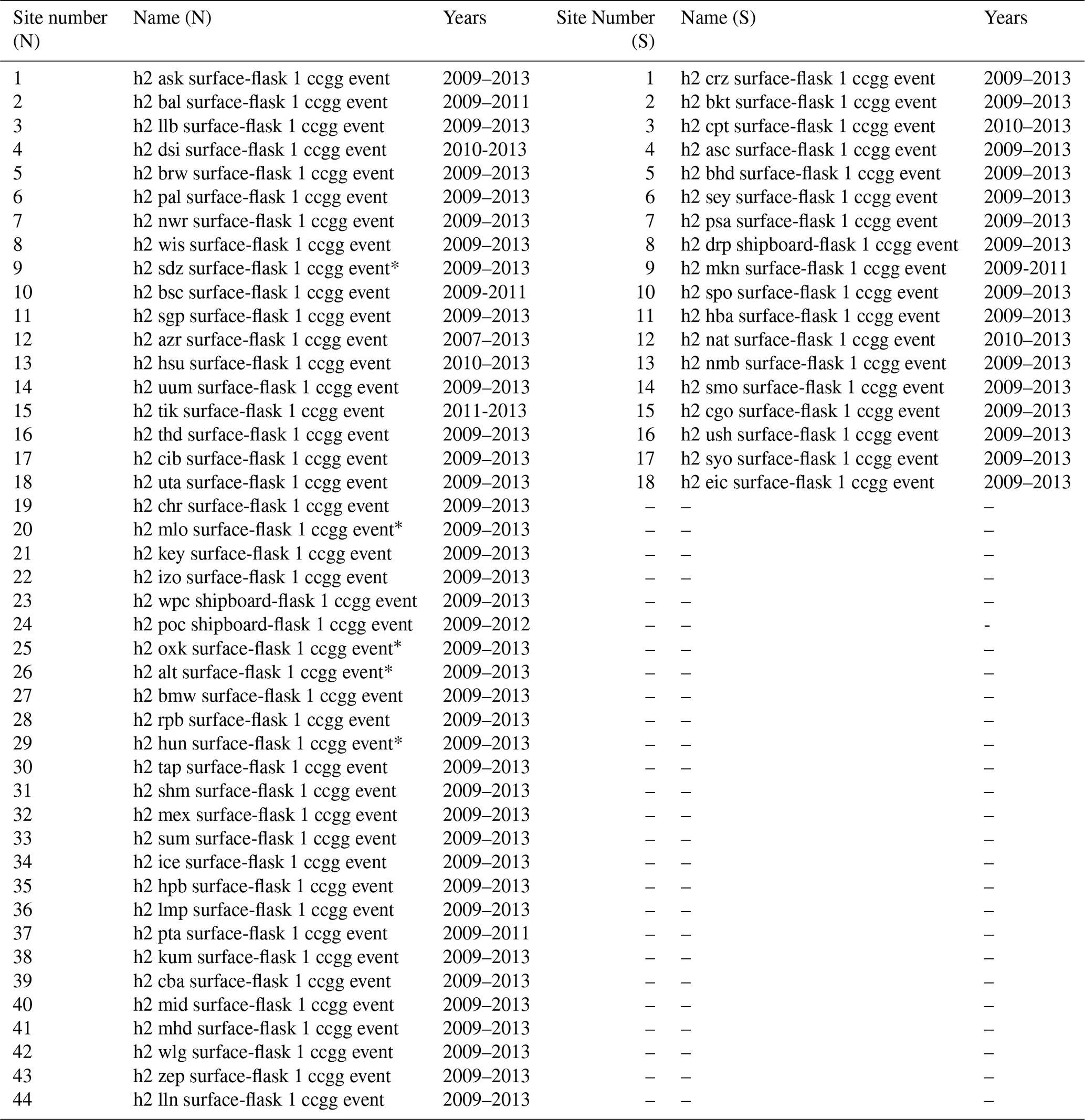
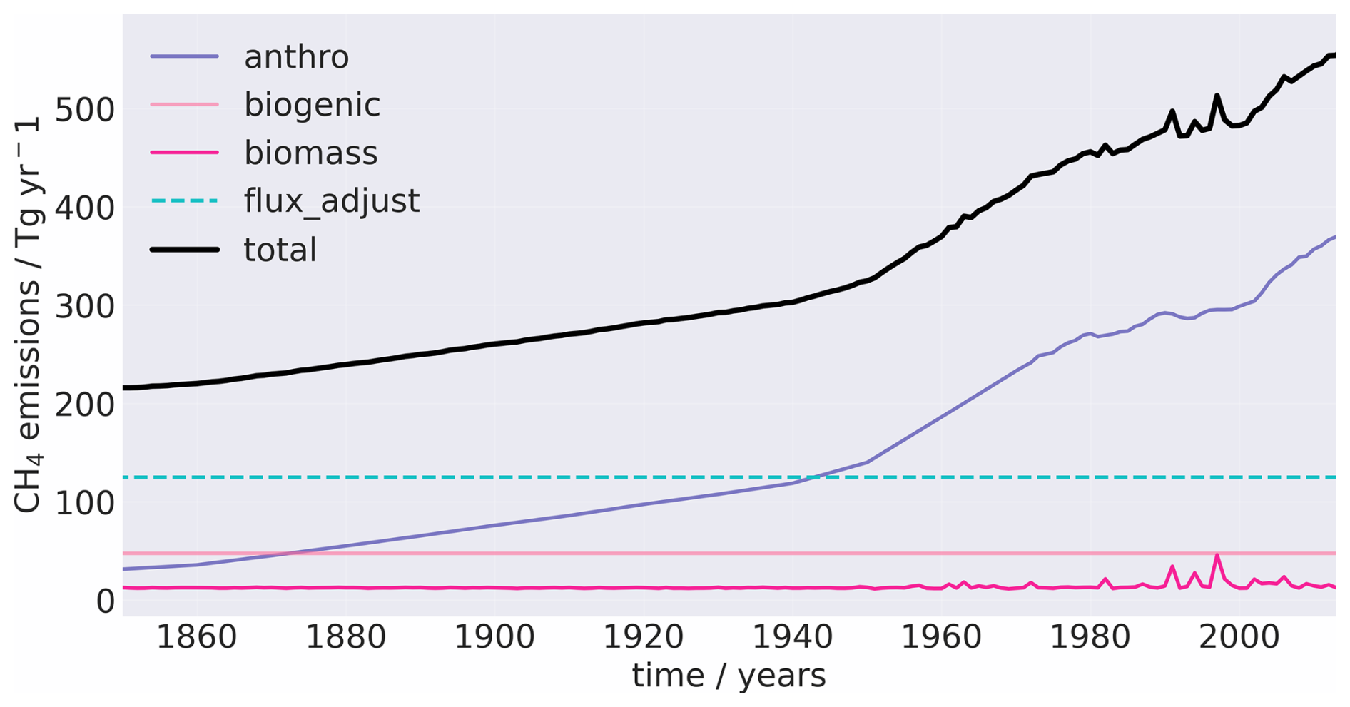
Figure A1 Yearly, globally averaged methane emissions from 1850–2014 (excluding wetlands). The flux adjustment is that used in the nudged simulations and is a total 124  CH₄ Tg yr⁻¹.

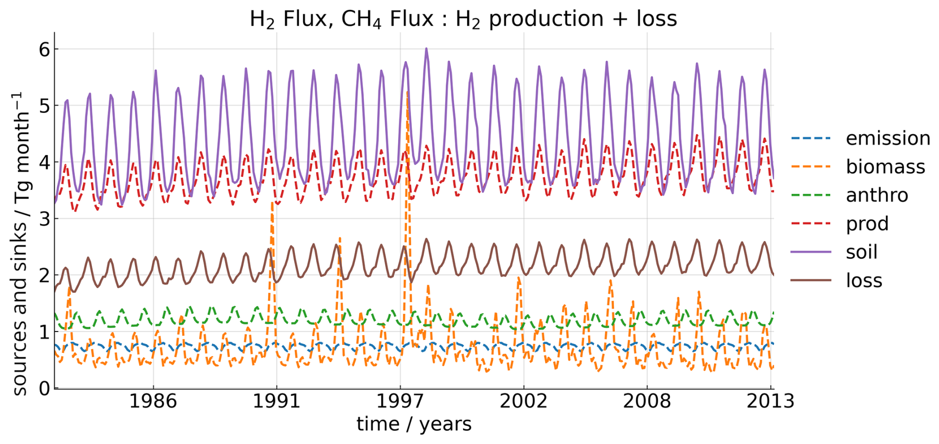
Figure A2 Globally averaged monthly hydrogen sources and sinks from 1982–2013. “emission” refers to the natural hydrogen emissions both from the ocean and land. “prod” and “loss” refers to the atmospheric chemical production and loss of H₂ respectively.

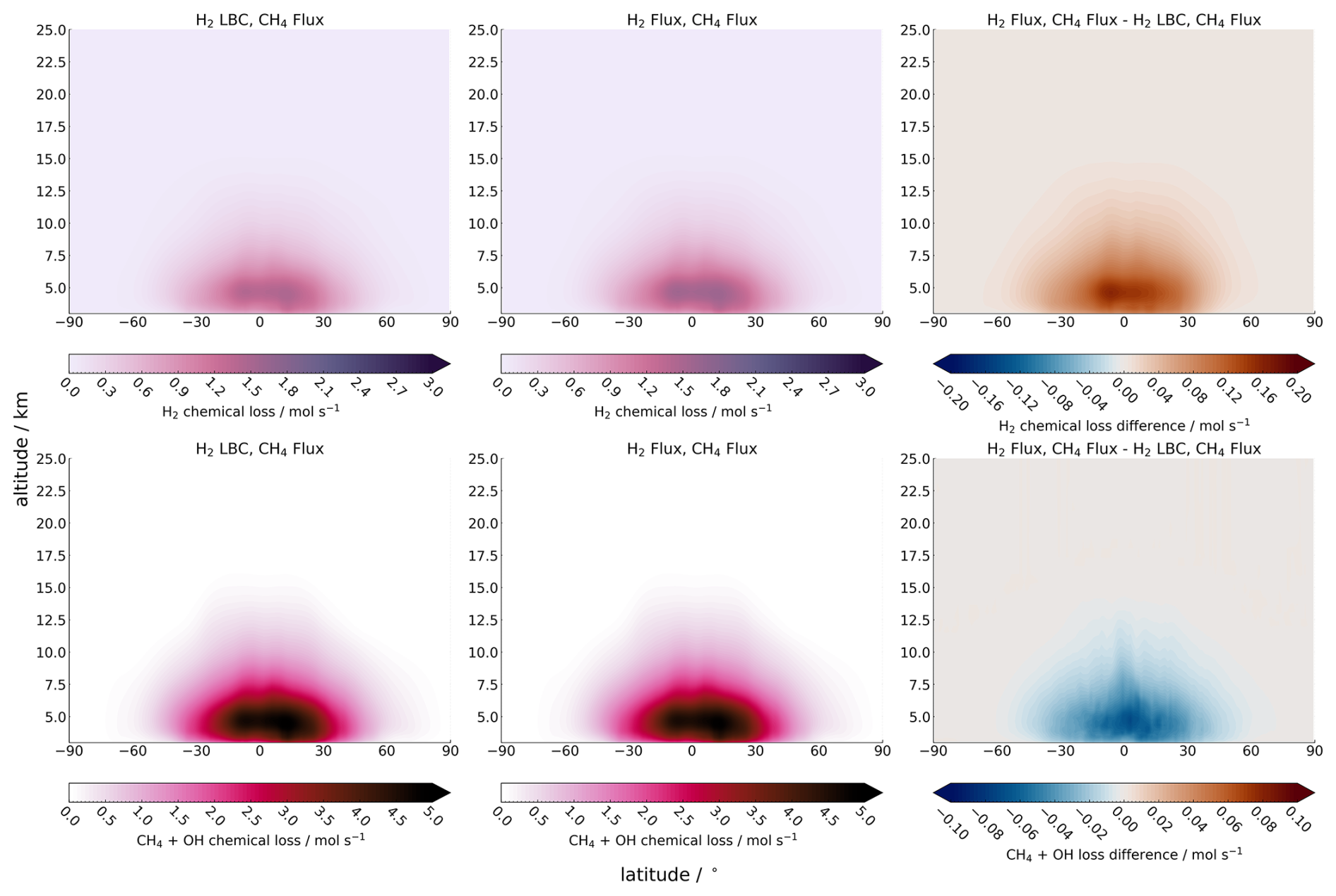
Figure A3 Zonally averaged (top) H₂ chemical loss and (bottom) CH₄ loss via OH for (left) TR-CH₄-flux simulation, (middle) TR-H₂CH₄-flux simulation, and (right) difference between the two (CH₄-flux − TR-H₂CH₄-flux) averaged between 2008–2013. Red (blue) shows an increase (decrease) from the TR-CH₄-flux. Note the non-linearity of scales.