An evaluation of the regional distribution and wet deposition of secondary inorganic aerosols and their gaseous precursors in IFS-COMPO preparatory to cycle 49R1

Secondary Inorganic Aerosol (SIA) makes up a considerable fraction of the total particulate matter exposure and, thus, is an important product from any forecasting system of atmospheric composition and air quality. The subsequent loss to the surface of SIA via dry and wet deposition determines the duration of the exposure time for humans and the extent of acidification imposed on sensitive ecosystems. Here we provide a description and evaluation of the most recent updates made towards aerosol production, aerosol scavenging and wet deposition components of the global Integrated Forecast System-COMPOsition (IFS-COMPO) chemical forecasting system, which is used as part of the Copernicus Atmosphere Monitoring Service. The implementation of the EQSAM4Clim simplified thermodynamic module in IFS-COMPO, for use in cycle 49R1, changes the efficacy of phase transfer of SIA precursor gases (sulphur dioxide, nitric acid and ammonia) which significantly impacts the respective SIA particulate concentrations by changing the fraction converted into SIA. Comparisons made against observational composites at the surface for Europe, the US, and Southeast Asia during 2018 show reductions in the global yearly mean bias statistics for both sulphates and nitrates. Updating the IFS-COMPO model towards cycle 49r1 increases both the burden and lifetime of sulphate and ammonium particles by one third. Coupling EQSAM4Clim into IFS-COMPO provides a better description of the partitioning between state phases involving ammonia and ammonium across regions, whereas changes for sulphate are minimal. For nitric acid and nitrates, the partitioning changes significantly, leading to lower particulate concentrations and a corresponding increase in gas-phase nitric acid with an associated improvement in surface nitrate. There is also a shift in the particle size distribution, with less nitrate production in the coarse mode and more in the fine mode. The impact on the total regional wet deposition values is generally positive, except for sulphates in the US and ammonium particles in Southeast Asia which are strongly influenced by the precursor emission estimates. This provides confidence that this update to IFS-COMPO has the ability to provide accurate deposition fluxes of S and N at global scale.

1 Introduction

Secondary Inorganic Aerosol (SIA) is found throughout the troposphere, where resident concentrations are dependent on Temperature (T), Relative Humidity (RH) and concentrations of inorganic precursor gases, namely water vapour (H₂O), sulphur dioxide (SO₂), ammonia (NH₃) and nitric acid (HNO₃). High concentrations of SIA contribute to total Particulate Matter that are smaller than using various predefined particle sizes namely: 1.0 µm (PM_1.0), 2.5 µm (PM_2.5) and 10 µm (PM₁₀) (Liu et al., 2022), and have detrimental effects on both human health and visibility (Sharma et al., 2020; Ting et al., 2022). The main types of SIA are ammonium sulphate ((NH₄)₂SO₄), ammonium bisulphate (NH₄HSO₄) and ammonium nitrate (NH₄NO₃). Once formed, the sulphates are very stable and deposit to the surface, whereas NH₄NO₃ is more unstable and can decompose back to the precursor gases (Feick and Hainer, 1954) depending on T and RH. These particles can be transported out of source regions subsequently influencing air quality in neighbouring countries (e.g., Vieno et al., 2014; Chang et al., 2022). Anthropogenic activity makes a significant contribution to SIA formation via the emission of NO_x (oxidised nitrogen in the form of NO and NO₂), NH_x (reduced nitrogen) and SO₂, where there has been a general trend of decreasing sulphur (S) and nitrogen (N) emissions in the EU, US and China (Tørseth et al., 2012; Aas et al., 2019; Benish et al., 2022; Jiang et al., 2022) resulting in an increasing fraction of SIA consists of NH₄NO₃. This results in a decrease in the lifetime of SIA, due to the increased instability of NH₄NO₃ due to variations in RH and temperature (e.g. Williams et al., 2015; Metzger et al., 2002, 2006), reducing the potential for reduced long-range transport out of the source regions (He et al., 2018).

At RH values above 50 %, SIA take up water and exist in a deliquescent state. At high RH values of 80 %–100 %, SIA formation is enhanced (Gao et al., 2020) therefore, under constant or changing emissions, SIA is likely to become more ubiquitous in a warming atmosphere. The hygroscopic growth of SIA alters both the optical properties (in terms of scattering and absorption) and interactions with gas-phase trace species via changes in pH (e.g. Jayne et al., 1990; Shi et al., 2019). The concentrated salt solution produced typically has higher ionic strength than cloud droplets with pH values ranging between −1 to 6 (Ault, 2020). The high solubility of SIA results in the scavenging into aquated aerosols and clouds being a dominant loss term. This has impacts in terms of the acidification of sensitive ecosystems and an increase in eutrophication due to high nitrogen loading in inland water bodies, which can result in the exceedance of critical loads for vegetation (e.g. Sun et al., 2020). The uptake of carbon to land is also enhanced with an increase in N loading (Holland et al., 1997; Reay et al., 2008). Once dissolved in solution, SIA dissociates efficiently into the respective ionic constituents (e.g. nitrate (NO${}_{\mathrm{3}}^{-}$), ammonium (NH${}_{\mathrm{4}}^{+}$) and sulphate (SO${}_{\mathrm{4}}^{=}\left)\right)$ whereas these anions/cations are deposited on land during precipitation events.

A distinct difference exists with respect to the main source terms for the various SIA species. For NO_x and NH_x species, particle formation is sensitive to the resident gas-phase precursor species, temperature, and RH, in the absence of aqueous phase droplets. For SO${}_{\mathrm{4}}^{\mathrm{2}-}$, production occurs almost exclusively in the aqueous phase after SO₂ is scavenged into cloud and fog, whose overall oxidation rate is dependent on the prescribed pH in solution. Recent studies have shown that the correct prescription of cloud pH is necessary to account for changes in SO${}_{\mathrm{4}}^{\mathrm{2}-}$ efficacy over long time scales for the determination of long-term trends with respect to resident concentrations (Thurnock et al., 2019; Myriokefalitakis et al., 2022). The representation of acidity in tropospheric aerosols and clouds ranges significantly across large-scale atmospheric models. The most simplistic representation is to use a fixed cloud water pH of between 5.0–5.6, thus effectively representing the impact of dissolved carbon dioxide (CO₂). A more accurate representation includes the influence of other dissolved species which either acidify (e.g. HNO_3, H₂SO₄) or buffer (e.g. NH₃) the pH of the solution once scavenged via irreversible uptake. This is the approach adopted in the Integrated Forecasting System with atmospheric composition extension (IFS-COMPO) for both cloud and precipitation. Other SO${}_{\mathrm{4}}^{\mathrm{2}-}$ production terms involving e.g. methyl-hydroperoxide (CH₃OOH) have been shown to be of secondary importance towards the total SO${}_{\mathrm{4}}^{\mathrm{2}-}$ production (Myriokefalitakis et al., 2022). The more buffering of solution due to the scavenging and dissolution of NH₃, the faster the conversion rate as dictated by the rate of reaction of HSO${}_{\mathrm{3}}^{-}$ being less than that for SO${}_{\mathrm{3}}^{=}$ (Warneck, 1988).

One dominant loss term for SIA is wet deposition in precipitation to the surface. Previous global tropospheric modelling studies have been performed focusing on the temporal accuracy and yearly deposition totals at continental scale for NH_x and SO_x (Zhang et al., 2012; Kanakidou et al., 2016; Ge et al., 2021), as well as multi-model intercomparison studies to examine the variability across different models and the main assumptions causing such differences (Dentener et al., 2006; Tan et al., 2018). The accuracy of any model towards capturing the correct wet deposition terms is a balance between the accuracy of the precursor emission inventory, the distribution of the cloud liquid water content (defining the cloud Surface Area Density, SAD), the representation of the formation and distribution of aerosol particles, the extent of phase-transfer and the parametrizations adopted for describing dry/wet deposition to the surface.

The IFS-COMPO model is a large-scale global model used for operational analyses and air quality forecasts (Rémy et al., 2024) used in the Copernicus Atmosphere Monitoring Service (CAMS; Peuch et al., 2024). This service provides forecasts and reanalysis of trace gases and aerosols for the purpose of informing national service providers and policy makers. It currently provides chemical/aerosol forecast products, among them Ozone (O₃), Nitrogen Dioxide (NO₂), SO₂, PM_2.5, PM₁₀ and Aerosol Optical Depth. One focus of the recent updates made to IFS-COMPO was the reduction of biases and increase in correlation for aerosol products against observations (Rémy et al., 2024). Reduced and oxidised nitrogen deposition can also be future CAMS products which will benefit from the improved speciation between gaseous and particulate nitrogen.

In this paper we present an analysis of the regional performance of IFS-COMPO Cy48r1 and the version used for developing Cy49r1 (hereafter referred to as pre-cy49r1) towards the surface distributions N and S gaseous precursors for SIA and the associated particle concentrations and distributions as evaluated against ground based observation networks, with special focus on the application of latest update of EQSAM4Clim (Metzger et al., 2024) in the global chemical forecasting model IFS-COMPO pre-Cy49r1. This work is both parallel and complementary to the recent evaluation of the performance of IFS-COMPO Cy48r1 and pre-Cy49r1 with respect to regional PM_2.5 distributions and Aerosol Optical Depth presented in Rémy et al. (2024). The influence on regional wet and dry deposition terms is subsequently evaluated to assess the application of both EQSAM4Clim (Metzger et al., 2024) and the deposition schemes. In Sect. 2 we provide details of the IFS-COMPO simulations used, a brief description of the latest model updates and emissions used. In Sect. 3 we describe the observational networks against which the surface evaluations are performed for the precursor gases and resulting SIA particulates. In Sect. 4 we provide details of the changes in regional surface concentrations of precursor gases and associated particulates and regional yearly mean statistics and in Sect. 5, we compare the yearly mean wet deposition fluxes against observations for Europe, the US and Southeast Asia and discuss improvements. Finally, in Sect. 6 we present some further discussion and conclusions from our study.

2 General information on the most recent IFS-COMPO versions

The IFS-COMPO global composition model (previously known as C-IFS) is used for operational air quality analyses and forecasts as part of CAMS. The modelling and data assimilation framework is regularly updated. During 2023 IFS-COMPO was based on the Cy48r1 version of IFS (https://www.ecmwf.int/en/elibrary/81374-ifs-documentation-cy48r1-part-viii-atmospheric-composition, last access: 20 February 2024), Since end of 2024, IFS-COMPO has moved to the pre-Cy49r1 version. IFS-COMPO pre-Cy49r1 has been shown to improve on the evaluated biases simulated in previous cycles for key products such as O₃ and NO₂ (https://atmosphere.copernicus.eu/eqa-reports-global-services, last access: 17 February 2025). Several updates were introduced in Cy49r1 to improve the aerosol component, the description of wet deposition and the representation of pH in clouds and aerosols. These include the application of the EQSAM4Clim approach and other developments associated with cloud scavenging (Metzger et al., 2016, 2024; Rémy et al., 2024). For brevity, we only provide a brief description of the updates in Cy49r1 relevant to this study. Further details are available in Rémy et al. (2024), which also includes a schematic representation of the model.

2.1 Updates in IFS-COMPO in pre-Cy49r1

IFS-COMPO Pre-Cy49r1 is built on the previous operational cycle (Cy48r1) and contains 8 distinct aerosol types with multiple bins for size segregation, namely sea salt, desert dust, organic carbon, black carbon, SO${}_{\mathrm{4}}^{=}$, fine and coarse NO${}_{\mathrm{3}}^{-}$, NH${}_{\mathrm{4}}^{+}$ and Secondary Organic Aerosol. For pre-Cy49r1 updates have been made to the aerosol component of the model in the form of modifying both the description and properties of desert dust and sea-salt, the aging of Carbonaceous aerosol and an update to the aerosol optics by changing the assumptions used for the SO${}_{\mathrm{4}}^{=}$ aerosol when referencing the lookup table for Mie scattering. This impacts the resident lifetimes, radiative properties and the long-range transport for each of the aerosol species. The modifications to the description of the aerosol optics have been shown to improve the simulation of Aerosol Optical Depth (AOD) and Ångström exponent when compared against regional observations (Rémy et al., 2024). The gas-phase chemistry, photolysis and dry deposition are identical to that used in Rémy et al. (2024) and as described in Williams et al. (2022). For brevity, and that this study is only concerned with soluble aerosols, we refer the reader to Rémy et al. (2024) for more explicit details related to the other aerosol types.

For pre-Cy49r1 there has been an integration of the aerosol and chemistry components in the code to make them more consistent, where both the sulfur and nitrogen cycles are now represented through the aerosol module (for particulate species) and the chemistry module (for gaseous species and aqueous SO${}_{\mathrm{4}}^{=}$ production). The aerosol module also provides additional input to the chemistry module to better represent heterogeneous reactions (via Surface Area Density (SAD)) and the effects of aerosols on photolysis rates. The extent of gas–particle partitioning and conversion via heterogeneous reactions on dust and sea-salt particles are outlined in Rémy et al. (2019), as based on the work of Hauglustaine et al. (2014). In Cy48r1, the first version of the EQuilibrium Simplified Aerosol Model (EQSAM; Metzger et al., 2002) was implemented for the calculation of e.g. NH₄NO₃ concentrations. These parameterizations rely on meteorological data provided by IFS, as well as gaseous precursors such as HNO₃ and NH₃ from the chemistry module. The gas–particle partitioning scheme estimates compound production through the neutralization of HNO₃ by NH₃ left over after the neutralization of H₂SO₄. It also accounts for the formation of specific compounds from heterogeneous reactions of HNO₃ with calcite (found in dust aerosol) and sea-salt particles.

In IFS-COMPO pre-Cy49r1, EQSAM4Clim is used to estimate the gas/particle partitioning of the HNO₃-NO${}_{\mathrm{3}}^{-}$ and NH₃-NH${}_{\mathrm{4}}^{+}$ couples and to provide an estimate of the aerosol pH. The pH of aqueous solutions, aquated aerosols and precipitation is now updated each time-step using the EQSAM4Clim approach accounting for additional cations (Ca²⁺, Mg²⁺, Na⁺, K⁺), anions (SO${}_{\mathrm{4}}^{=}$, HSO${}_{\mathrm{4}}^{-}$, NO${}_{\mathrm{3}}^{-}$, Cl⁻) and their solute interactions, whose methodology is comprehensively described in Metzger et al. (2002, 2016, 2024). This replaces the original estimate of the pH of the solution determined by summing the contributions from dissolved CO₂ and strong acids (HNO₃, HSO${}_{\mathrm{3}}^{-}$, H₂SO₄, NO${}_{\mathrm{3}}^{-}$ and Methane Sulfonic Acid) which is buffered by dissolved NH₃. The contribution towards the pH of the solution of dissolved Formic and Acetic acid (HCOOH and CH₃COOH, respectively) are also now accounted for in pre-Cy49r1, which has been shown to contribute to the pH in cloud droplets (Shah et al., 2020). This impacts the phase-transfer, speciation, and subsequent aqueous-phase oxidation of SO₂ in cloud droplets (thus impacting SO${}_{\mathrm{4}}^{=}$). Also, the loss of gas-phase species such as e.g. H₂O₂ and the corresponding formation of SIA particles is affected. Note that both the original (Cy48r1) and updated (pre-Cy49r1) approaches account for the most dominant gaseous contributions towards the pH of the solution, namely SO₂, HNO₃ and NH_3. This means that differences imposed in cloud pH are naturally less than the associated changes in aerosol pH. The aqueous phase oxidation of SO₂ by transition metal ions (Fe²⁺, Mg²⁺) is not currently accounted for but considered a minor pathway.

Below cloud scavenging of gaseous precursors is also affected by the pH of solution (e.g. Seinfeld and Pandis, 2006). In Cy48r1 fixed values for cloud pH are used over land (pH = 5.0) and ocean (pH = 5.6), thus only providing limited variability with respect to regions affected by both high and low emissions. In pre-Cy49r1 this has been updated such that the calculator of the pH is coupled to resident trace gas and aerosol concentrations to improve consistency within IFS-COMPO and to provide variable scavenging rates dependent on tropospheric composition.

In Cy48r1, the wet deposition routines for aerosols and chemistry in IFS-COMPO are distinct, though both utilise a scheme adapted from Luo et al. (2019). To ensure a consistent approach between aerosol and trace gases wet deposition, and to simplify code maintenance, these separate implementations have been merged into a unified routine. This new routine now represents the wet deposition processes for both aerosols and chemical species and is called with either chemical or aerosol tracers as input. As with Cy48r1 and previous versions, the wet deposition routine in pre-Cy49r1 is executed twice: once for large-scale precipitation and once for convective precipitation. In the case of convective precipitation, the assumed precipitation fraction has been standardised to 0.05 (whereas in Cy48r1 a value of 0.1 was used for chemistry scavenging and 0.05 for aerosol scavenging).

Additional upgrades have been made for aerosol wet deposition as follows: (i) The aerosol activation parameterization of Verheggen et al. (2007) has been implemented. This parameterization estimates the fraction of aerosols that can be scavenged through in-cloud processes as a function of temperature. It is applied to mixed clouds, specifically for temperatures between the freezing point and 233 K. For temperatures above 0 °C, the consistency of the parameters determining the fraction of aerosols subject to in-cloud wet deposition with the results of the Verheggen parameterization has been verified. (ii) For below-cloud scavenging of aerosol species, the scavenging rates have been updated to reflect the particle size dependency more accurately as described by Croft et al. (2009). This update includes adjustments to the below-cloud scavenging parameters, which describe the efficiency with which aerosols are removed by rain and snow, depending on the species and the assumed size distribution.

2.2 Setup of model simulations

The IFS-COMPO simulations used for evaluating the impact of IFS-COMPO atmospheric composition upgrades proposed for pre-Cy49r1 on tropospheric composition, precursor gases, particle distributions and wet deposition terms employ both the IFS cycles Cy48r1 and pre-Cy49r1. Here, pre-Cy49r1 denotes the IFS-COMPO Cy48r1 including updates of aerosol/chemistry modules which are now applied in IFS pre-Cy49r1. The meteorological component is the same between simulations and corresponds to Cy48r1. Still, marginal differences may occur between simulations due to a coupling of gases and aerosol with radiation, which is active by default. The simulations presented here are for the year 2018, with a one-month spin-up period. The vertical resolution uses 137 individual model levels and a horizontal resolution of T_L511, corresponding to approx. 0.4° × 0.4° (with further details being given at https://confluence.ecmwf.int/display/UDOC/L137+model+level+definitions, last access: 25 November 2025). The experiments do not include the data assimilation of observations, meaning that although the changes shown will not be directly visible in the final operational forecast, they will influence the resulting skill scores for e.g. PM_2.5. Meteorology is initialised every 24 h based on ERA5 reanalysis data, i.e. IFS-COMPO is run in a cyclic forecast mode. A 15 min chemical time-step is used for solving a modified version of CB05 tropospheric chemistry (Williams et al., 2022), excluding active stratospheric chemistry for efficiency (with this study being focused on changes at the surface). Three-hourly 3D global output is used for the analysis and aggregated into weekly, monthly, and yearly mean values.

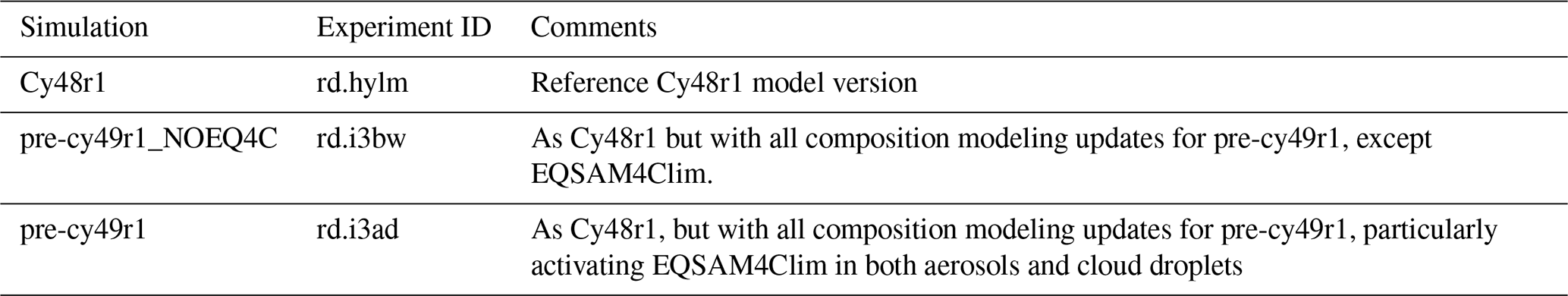
The details of the experiments are summarised in Table 1. The Cy48r1 reference simulation pertains to the 48R1 version of IFS-COMPO while the pre-Cy49r1 simulation is based on the version described in Rémy et al. (2024), which is Cy48r1 updated with new components for use in future versions of IFS-COMPO. The pre-Cy49r1_NOEQ4C simulation is identical to the pre-Cy49r1 simulation, except the EQSAM4Clim module (Metzger et al., 2024) is deactivated. For future reference, the experiment identities on the ECMWF Multiversion Asynchronous Replicated Storage system (MARS) are hylm (Cy48r1), i3bw (pre-Cy49r1_NOE4C) and i3ad (pre-Cy49r1). These three simulations use a configuration, and emissions as those used for the simulations presented in Rémy et al. (2024) for evaluating PM. We select the year 2018 to provide further evaluation which is complimentary to the results presented for 2019 in Rémy et al. (2024).

Table 1 Definitions of the IFS-COMPO simulations used in this study. The experiment ID's can be used to retrieve the original data from the MARS archiving system hosted at ECMWF.

The anthropogenic emissions adopted in these configurations are taken from CAMS_GLOB_ANT v5.3 (Soulie et al., 2024), biogenic emissions taken from the CAMS_GLOB_BIO v3.1 dataset (Sindelarova et al., 2022; http://eccad.aeris-data.fr/, last access: 20 November 2025) and biomass burning emissions taken from GFAS v1.2 (Kaiser et al., 2012). All emissions are provided at 0.1×0.1 resolution at a monthly frequency, except for the biomass burning emissions which are prescribed daily. For biomass burning and anthropogenic emissions from specific sectors vertical profiles are used representing pyrogenic convection or industrial stack heights, with other emissions being applied in the lowest model level. A diurnal cycle is imposed for isoprene and biomass burning emissions to capture either photolytic activity or the tropical burning cycle. Volcanic outgassing of SO₂ is also included based on Andres and Kasgnoc (1998). For di-methyl sulphide (DMS) oceanic emissions are based on Kloster et al. (2006) i.e. not coupled to sea surface temperature which controls biogenic activity (Deschaseaux et al., 2019). Moreover, direct production of SO${}_{\mathrm{4}}^{=}$ and HNO₃ in hot shipping exhausts is not accounted for (e.g. von Glasow et al., 2003).

3 Observations

For SO₂(g) $/$ SO${}_{\mathrm{4}}^{\mathrm{2}-}$, NH₃(g) $/$ NH${}_{\mathrm{4}}^{+}$ and HNO₃(g) $/$ NO${}_{\mathrm{3}}^{-}$ evaluation in Europe we compare IFS-COMPO model output against data taken from the EMEP measurement network as stored on the EBAS data archive (EMEP, Tørseth et al., 2012; https://ebas.nilu.no/, last access: 6 June 2025) using a composite of 49 individual stations located in 10 different countries, as shown in the top panel of Fig. A1 in the Appendix. We chose sites which monitor both the pre-cursor gases and associated SIA simultaneously to ensure valid comparisons. The sampling sites are located mostly in northern and eastern Europe, but co-location of model output means the comparison is still valid., albeit having less representation for southern Europe. For the US we compare model output aggregated on a weekly basis against data provided at locations included in the Clean Air Status and Trends Network (CASTNET; https://www.epa.gov/castnet, last access: 6 June 2025) using a composite of 92 individual stations distributed across the US. The distribution of the US measurement sites is shown in the middle panel of Fig. A1 in the Appendix. For NH₃(g) not direct measurements are available from the CASTNET database, therefore we compare against both weekly and yearly mean values as derived from sites located near CASTNET stations (within 0.5° radius) i.e. 92 of the current 106 sites in the Ammonia Monitoring Network (AMoN, https://nadp.slh.wisc.edu/networks/ammonia-monitoring-network/, last access: 6 June 2025). No filtering has been applied to any of the observational data used in this study. Unfortunately conducting a similar analysis in Southeast Asia was not possible owing to the unavailability of both precursor and SIA weekly measurements.

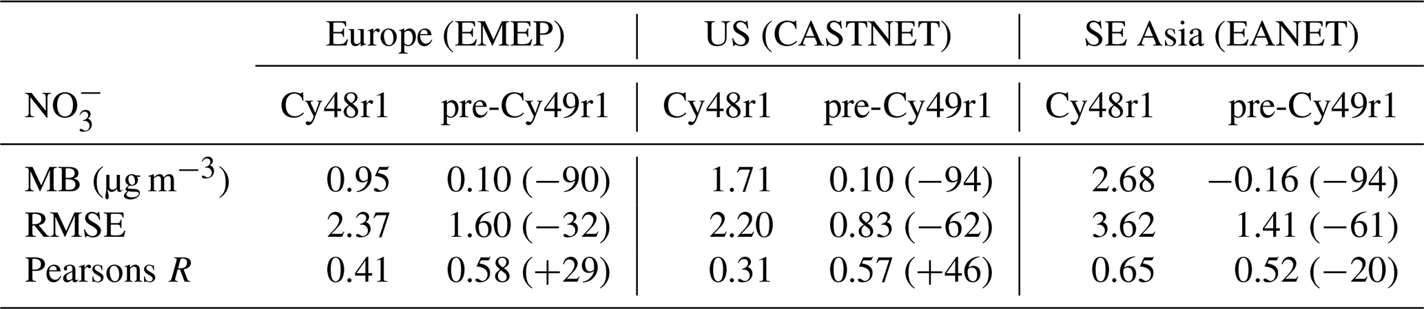
For evaluating the SIA particle concentrations, we use available data from the EMEP (Europe), CASTNET (US) and the Acid Deposition Monitoring Network in East Asia (EANET, https://www.eanet.asia/, last access: 6 June 2025; S. E. Asia) for SO${}_{\mathrm{4}}^{\mathrm{2}-}$, NH${}_{\mathrm{4}}^{+}$ and NO${}_{\mathrm{3}}^{-}$. The EANET network includes 41 individual stations covering a wide region, whose location is shown in the bottom panel of Fig. A1 in the Appendix. Although we use all the observations provided in each database, the distribution is non-homogeneous, with those in EMEP being clustered towards northern Europe and those in Southeast Asia spanning a large area from eastern China to Japan. The locations of the stations used for evaluation are also shown (black circles) on the corresponding figures associated with regional and spatial validation.

For the wet deposition totals we use data taken from the same measurement networks and sampling frequency as those used for evaluating the gaseous precursors and SIA (EMEP, CASTNET, EANET) thus removing any differences potentially introduced by spatial sampling which would complicate the comparisons discussed here. Although seasonal variability is of interest, the EANET wet deposition totals are only provided as yearly mean values placing constraints on the sampling frequency used for the analysis. Therefore, the averaging period chosen for the evaluation is constrained by the frequency and availability of the data from Southeast Asia. All statistical metrics represent spatio-temporal averages unless otherwise noted, combining all station-time pairings into a single evaluation vector per region and species. No filtering of the data was performed before making the comparisons.

4 The influence of pH on SIA chemical precursors and particulates

The efficacy of SIA formation is strongly governed by the resident concentrations of the gaseous precursors. Therefore, changes imposed with respect to the parameterizations used for simulating particle formation also have an associated feedback effect on the precursors, due to changes in the fractional uptake governed by the solute pH. In this section, we evaluate the temporal and regional distribution and biases of both gaseous precursors (SO₂, NH₃, HNO₃) and associated SIA (namely SO${}_{\mathrm{4}}^{=}$, NH${}_{\mathrm{4}}^{+}$, NO${}_{\mathrm{3}}^{-}$) simulated by IFS-COMPO for Europe, the US and Southeast Asia. Mixing ratios and particle concentrations are strongly influenced by the description and distribution of the primary emission sources, meteorology, dry/wet deposition, aerosol pH (for NH_x and NO_x) and atmospheric transport. To investigate the ability of IFS-COMPO towards capturing the observed distributions, we compare both weekly and yearly mean composites for Cy48r1 and pre-Cy49r1 against the corresponding values derived from in-situ measurements.

4.1 SO₂ and SO${}_{\mathrm{4}}^{=}$

Figure 1 shows the regional monthly mean distributions in surface SO₂ mixing ratios for July and December 2018 for Cy48r1, along with the relative percentage differences between Cy48r1, pre-Cy49r1_NOEQ4C and pre-Cy49r1. When comparing the spatial distributions across regions, Europe exhibits the lowest SO₂ mixing ratios in Cy48r1, where the region has undergone strong mitigation practices over the last decades (e.g. Vestreng et al., 2007). The maps for July show higher mixing ratios towards the east, with a significant contribution from shipping in the Mediterranean and the English Channel. For December, the highest mixing ratios occur over the continent, most notably in Germany and Poland. For the US, a stark east-west gradient exists as governed by the continental distribution in anthropogenic emissions, with higher emissions towards the East Coast, again with a seasonal signature. Maximal surface mixing ratios are 5–10 times higher than those simulated for Europe distributed over a much larger area. As expected, China exhibits the highest regional mixing ratios of between 10–20 ppb over the entire country, which is approximately 20 times higher than those simulated for Europe for both months shown.

When comparing Cy48r1 against pre-Cy49r1_NOE4C there are reductions in [SO₂(g)] at the surface for all regions of between 0 %–10 %, resulting in limited increases in SO${}_{\mathrm{4}}^{\mathrm{2}-}$ production of a few percent due to changes other than those related to the application of EQSAM4Clim. This small increase in the SO${}_{\mathrm{4}}^{\mathrm{2}-}$ production is reversed when applying the EQSAM4Clim pH methodology (Metzger et al., 2024), where the conversion efficacy of SO₂ is faster at a more alkalinic pH. Table 2 provides the global budget terms for SO₂(g), which shows that in addition to primary emission, approximately one third of SO₂ in the troposphere comes from the oxidation of DMS by the hydroxyl radical (OH), with DMS originating from biogenic activity in the oceans.

In Cy48r1, approximately 20 % of SO₂ is oxidised in the gas-phase and 43 % in the aqueous phase, with the remaining 37 % being lost to surface via dry and wet deposition. This increase in gas-phase production via OH is linked to changes imposed by differences in O₃-NO_x reaction cycles near anthropogenic source regions which results in a small increase in O₃ of a few percent (not shown). The corresponding values for pre-Cy49r1_NOE4C show changes in the order of a few percent across terms, increasing the global burden by of SO₂(g) by 1.4 % mostly in the lower troposphere. For pre-Cy49r1 the application of EQSAM4Clim pH in cloud droplets reduces both the uptake and oxidation of SO₂ by reducing aquated sulphite ([SO${}_{\mathrm{3}}^{\mathrm{2}-}$]_aq, pKa(HSO${}_{\mathrm{3}}^{-})=\mathrm{7.2}$) and an enhancement of the gas-phase oxidation due to increased OH, resulting in more gas-phase production of H₂SO4. This is subsequently scavenged into solution further increasing solution acidity (lowering pH values) in case of excess SO${}_{\mathrm{4}}^{\mathrm{2}-}$ (insufficient cations to completely neutralise all SO${}_{\mathrm{4}}^{\mathrm{2}-}$).

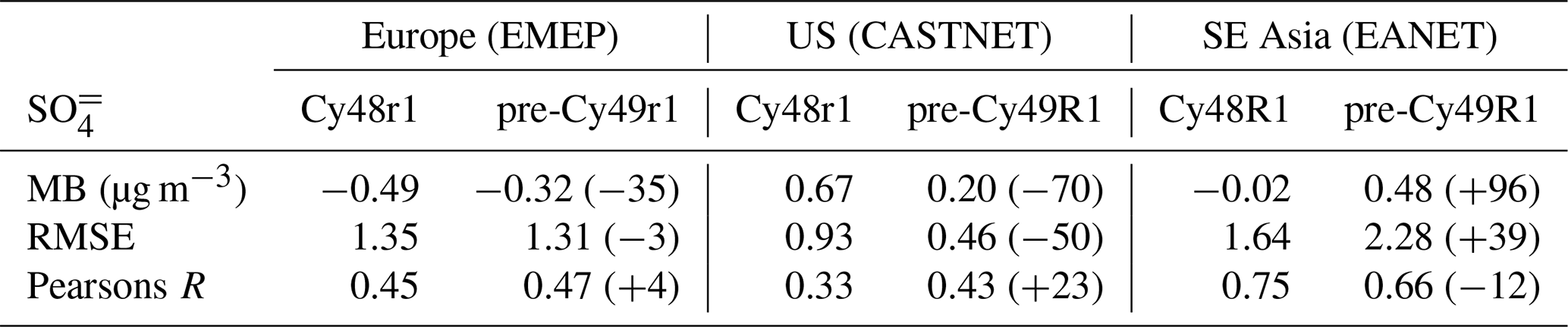
Figure 2 shows a comparison of weekly [SO₂(g)] and [SO${}_{\mathrm{4}}^{\mathrm{2}-}$] surface composites as simulated in IFS-COMPO against weekly composites of measurements taken from the EMEP measurement network (top left panel). For SO₂(g) a consistent positive bias exists for the entire year across all IFS-COMPO simulations suggesting emission estimates which are high. Surface concentrations exhibit around 100 % positive bias, increasing to almost 200 % during wintertime. The variability in the observational means (grey shaded area) does indicate that the simulated increase in surface [SO₂(g)] during wintertime does occur at some of the measurement sites. The corresponding observational means of [SO${}_{\mathrm{4}}^{\mathrm{2}-}$] show that there is higher weekly variability during wintertime than summertime, with concentrations ranging typically between 1.0–2.0 µg m⁻³. This significant wintertime weekly variability is simulated well by IFS-COMPO across all simulations, where both Cy48r1 and pre-Cy49r1 exhibit significant positive biases of 0.5–1.0 µg m⁻³. Surprisingly, pre-Cy49r1_NOE4C has the lowest bias during wintertime of around 0.2–0.5 µg m⁻³. For pre-Cy49r1, there is an increase in surface [SO${}_{\mathrm{4}}^{\mathrm{2}-}$] by approximately 10 %–25 %, albeit with a significant negative bias of around 0.8–1.5 µg m⁻³. During summertime, the weekly variability in the observed weekly means is insignificant. All simulations capture this limited variability, with differences across simulations being around 0.1-0.2 µg m⁻³. Due to the primary source term of SO₂ being direct emissions, the high [SO₂(g)] simulated for Eastern Europe suggests a local overestimate (cf. Fig. 1).

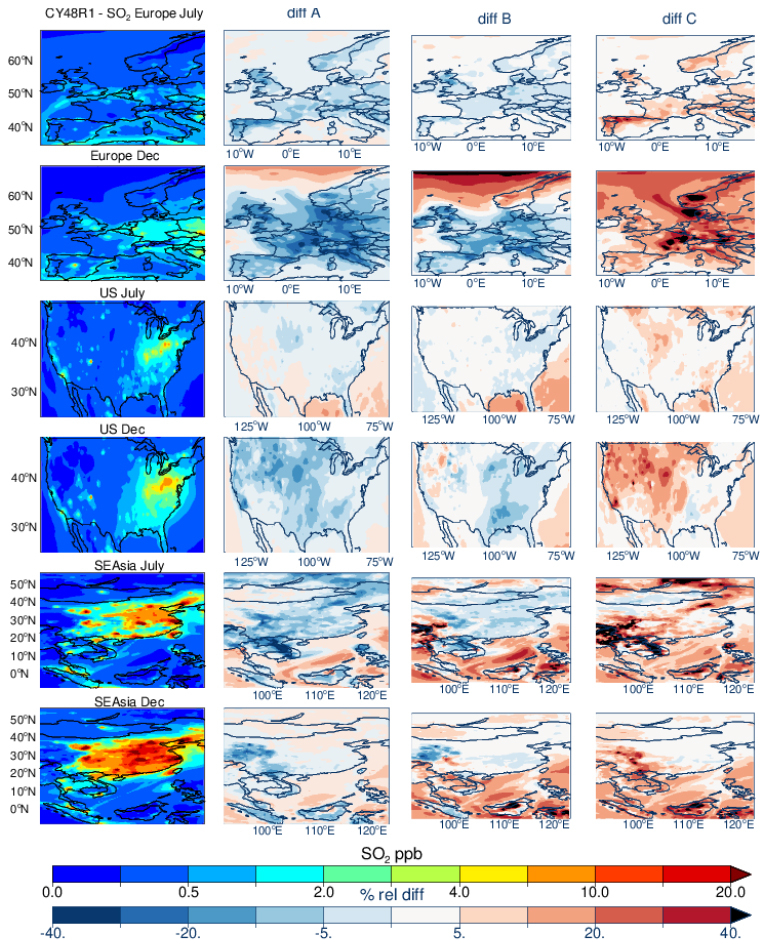
Figure 1 The horizontal monthly mean distribution for surface SO₂ for Cy48r1 for July and December 2018 for Europe (top), the United States (middle) and Southeast Asia (bottom). The corresponding relative differences when compared against the other simulations. Panel definitions: Diff A = (pre-cy49r1_NOEQ4C-Cy48r1)$/$Cy48r1; Diff B = (pre-cy49r1-Cy48r1)$/$Cy48r1 and Diff C = (pre-Cy49r1-pre-Cy49r1_NOEQ4C)$/$Cy48r1.

Table 2 The tropospheric SO₂ budget in Tg S yr⁻¹ for 2018 as calculated by Cy48r1, pre-Cy49r1_NOE4C and pre-Cy49r1, with the associated percentage differences being provided in parentheses as e.g. ((pre-Cy49r1-Cy48r1)/Cy48r1) × 100. All global budget terms are closed.

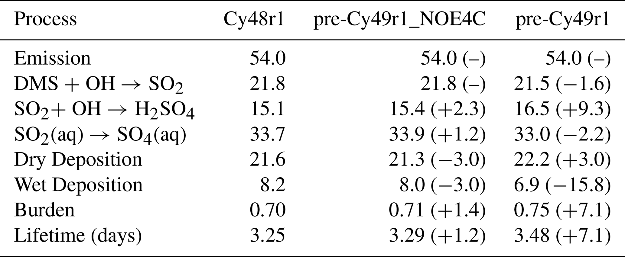
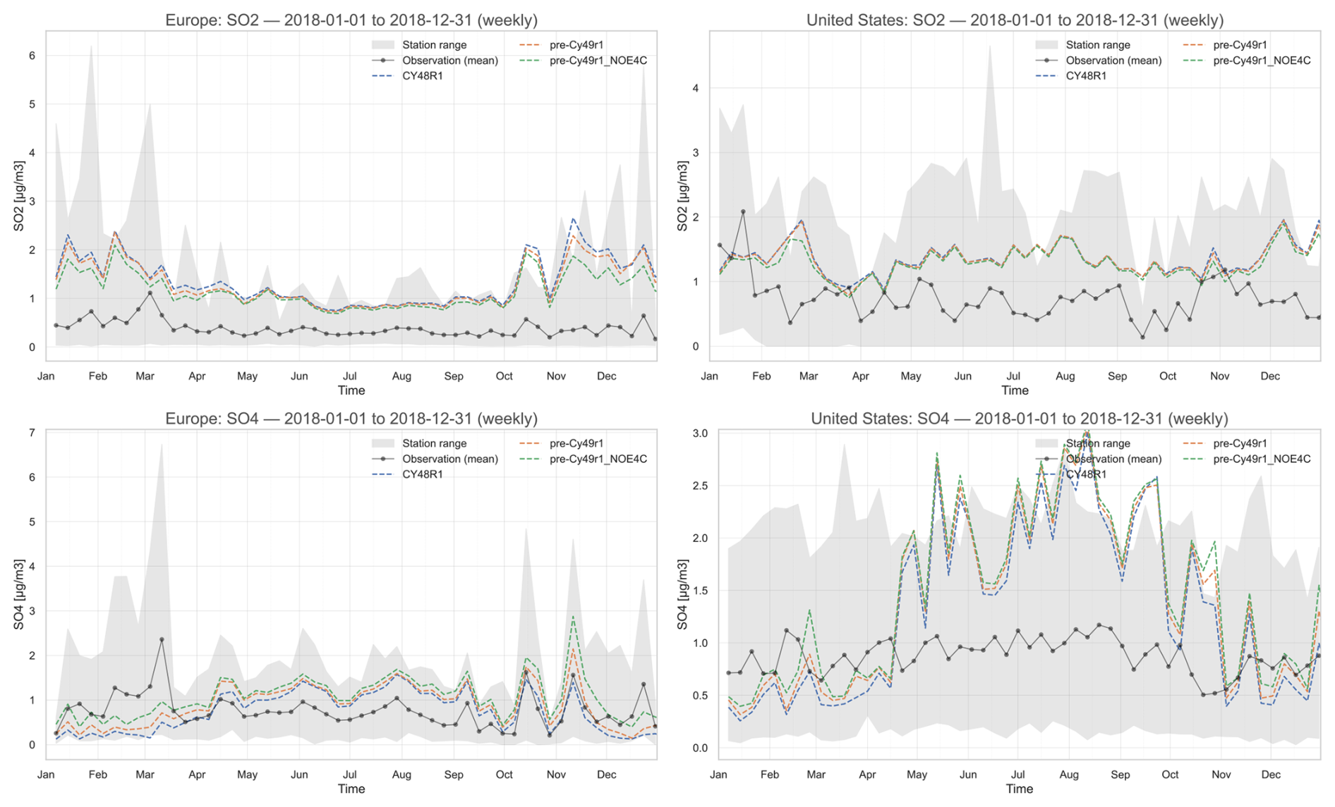
Figure 2 A comparison of weekly mean SO₂ and SO${}_{\mathrm{4}}^{\mathrm{2}-}$ for Europe (left panels; µg m⁻³) and the US (right panels) simulated in IFS-COMPO as compared against EMEP and CASTNET observational networks, respectively, for 2018. The sampling frequency of the data for SEAsia does not allow a corresponding weekly plot for this region. The grey band shows the station range (min–max) of observed weekly means at each time.

In the right-hand panels of Fig. 2 a similar comparison is made against weekly observational composites of surface [SO₂(g)] and [SO${}_{\mathrm{4}}^{\mathrm{2}-}$] from the CASTNET measurement network. As for Europe, no seasonal cycle exists in the observations of either surface [SO₂(g)] or [SO${}_{\mathrm{4}}^{\mathrm{2}-}$] with typical weekly mean values of around 0.7–1.0 µg m⁻³. For the wintertime, lower weekly MB occur for both pre-Cy49r1_NOE4C and pre-Cy49r1 as compared with Cy48r1, where the weekly variability is inverse of that seen in the observations. During the summertime much larger positive biases occur, reaching between 200 %–300 % across all IFS-COMPO simulations. Simulated [SO${}_{\mathrm{4}}^{\mathrm{2}-}$] exhibits a strong seasonal cycle despite no such increase in the simulated [SO₂(g)]. Although some small differences in the SO₂(g) weekly values occur between simulations, there is no improvement in pre-Cy49r1 with respect to the weekly MB. The positive summertime MB for SO₂ implies that there is either an overestimate in the regional source terms or an underestimate in the depositional loss term (cf. [SO${}_{\mathrm{4}}^{\mathrm{2}-}$] below)

Figure 3 shows the yearly means of surface [SO${}_{\mathrm{4}}^{\mathrm{2}-}$] for Cy48r1 and pre-Cy49r1 for Europe (top panels), the US (middle panels) and Southeast Asia (bottom panels). The changes in surface [SO${}_{\mathrm{4}}^{\mathrm{2}-}$] here are somewhat unaffected by the changes in PM_2.5 due to EQSAM4Clim that are shown in Rémy et al. (2024) for 2019, due to the dominant aqueous-phase production term (albeit with small increases due to the additional contribution from organic acids). One main difference for SO_x than either NH_x or NO_x, is that the gas-particle partitioning is dependent on cloud pH, dissolved O₃ and hydrogen peroxide (H₂O₂), where SO${}_{\mathrm{4}}^{\mathrm{2}-}$ production is irreversible.

For Europe, a sharp north-south gradient exists imposed by the variability in H₂SO₄ production between seasons, cloud cover for the wet production term and the distribution of the primary point sources for SO₂ emissions, although mitigation measures remove the increase in the emitted flux during the cold winter months associated with domestic heating (Veheggen et al., 2007). Simulated concentrations in Cy48r1 are lower in Scandinavia as compared with e.g. France, which results in a low bias of around 1 µg m⁻³ in e.g. Finland and around the Baltic, here related to missing shipping emissions of SO₂, which quickly converts to SO${}_{\mathrm{4}}^{\mathrm{2}}$ in the plume (Celik et al., 2020). For the other sites in Europe agreement is better with the low bias decreasing to approx. 0.5 µg m⁻³. One outlier exists for the most easterly station, which exhibits a significant high bias of 1.5 µg m⁻³. Comparing pre-Cy49r1 shows increases in the simulated surface [SO${}_{\mathrm{4}}^{\mathrm{2}-}$] of between 0.2–0.4 µg m⁻³, which leads to an improved bias. Only small improvements are made to the correlation coefficient due to identical emission estimates being used and EQSAM4Clim affecting SO_x the least, i.e., only indirectly through changes in pH.

For the US, the CASTNET observations show an east-west continental gradient in surface [SO${}_{\mathrm{4}}^{\mathrm{2}-}$] exists as determined by the distribution in the primary SO₂ emissions and transport (cf. Fig. 1). A significant transport component exists for SO${}_{\mathrm{4}}^{\mathrm{2}-}$, resulting in surface [SO${}_{\mathrm{4}}^{\mathrm{2}-}$] in the Marine Boundary Layer between 1.0–2.5 µg m⁻³, where transport dominates local surface [SO${}_{\mathrm{4}}^{\mathrm{2}-}$] produced from DMS oxidation (Simpson et al., 2014). For pre-Cy49r1 there is a reduction in surface [SO${}_{\mathrm{4}}^{\mathrm{2}-}$] at continental scale, with a decrease in the yearly MB from 0.67 to 0.20 µg m⁻³, with a corresponding increase in the correlation coefficient to 0.43, albeit remaining only rather weakly correlated. For the West of the US a positive MB is introduced for the rural background in pre-Cy49r1 of 0.5–0.7 µg m⁻³, with a contribution being transported from the east. Hence, reductions in the yearly MB primarily stem from improved agreement at Eastern US monitoring sites. That a positive MB of approx. 1–1.5 µg m⁻³ exists in the yearly mean values around Kentucky/Tennessee suggests that the local SO₂ emission estimates are too high (see Discussion in Sect. 5).

For Southeast Asia, the scarcity of sampling sites in the EANET network results in a less robust evaluation. Many sampling sites are located at coasts rather than inland, thus the influence of changes at coastal regions has an influence on the regional statistics. Higher primary SO₂ emissions occur on the land. Therefore, any positive MB near source regions is not included in the statistics; the results shown here for surface SO${}_{\mathrm{4}}^{\mathrm{2}-}$ should be considered lower limits. The long-range transport of SO${}_{\mathrm{4}}^{\mathrm{2}-}$ in Asia has been shown to somewhat neutralise national SO₂ mitigation measures taken in e.g. Taiwan and South Korea. This originates from changing trends in SO₂ emission from mainland China as captured by EANET measurement sites (Chang et al., 2022). For Cy48r1 the yearly mean statistics show an exceptionally low MB and a good correlation coefficient of 0.75. For pre-Cy49r1 there is a significant degradation, where the MB increases to 0.48 µg m⁻³ showing a trend in the performance for SO_x that is like the US. Notably, the more remote sampling stations (e.g. oceanic) exhibit regional negative biases (approx. −0.7 µg m⁻³) whereas those situated near Mongolia and South Korea agree well with low MB values. For Thailand and Vietnam there are typically large MB values, suggesting regional SO₂ emission estimates are too high. Unfortunately, there are no in-situ measurements available for better quantification. The correlation coefficient degrades in pre-Cy49r1 compared to Cy48r1 towards 0.66. Overall, the improvements are mixed for the SO₂ − SO${}_{\mathrm{4}}^{\mathrm{2}-}$ couple and much less pronounced compared to the other SIA.

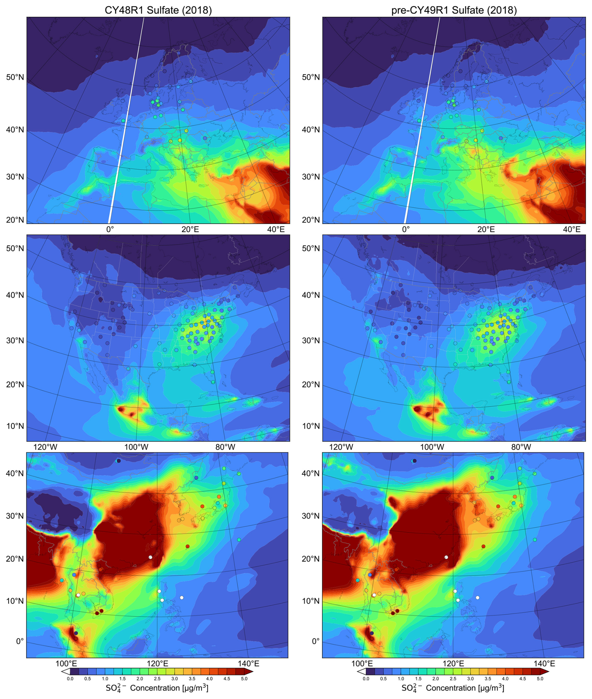
Figure 3 Comparisons of yearly mean [SO${}_{\mathrm{4}}^{\mathrm{2}-}$] simulated at the surface in Cy48r1 and pre-Cy49r1 when compared against measurements for the three selected regions during 2018 (µg m⁻³). The corresponding regional statistics are provided in Table 3. Site locations and observed values, taken from the EMEP, CASTNET and EANET networks respectively, are shown in circles.

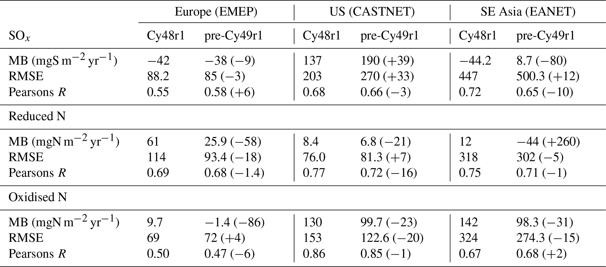
Table 3 The yearly MB, RMSE and Pearsons R values for the comparisons of the daily (EMEP, Europe), weekly (CASTNET, US) and yearly (EANET, Southeast Asia) mean regional distributions and concentrations of surface SO${}_{\mathrm{4}}^{\mathrm{2}-}$ as compared against composites assembled from the observations for 2018 shown in Fig. 3 for Europe, the US and Southeast Asia. Percentage differences are calculated as ((pre-Cy49r1-Cy48r1)/Cy48r1) × 100 and given in parentheses.

4.2 NH₃ and NH${}_{\mathrm{4}}^{+}$

The regional distribution of surface NH₃ for 2018 in the three chosen global regions and the resulting changes for pre-Cy49R1_NOE4C and pre-Cy49r1 are shown in Fig. 4. Although there is a declining trend in European regional NH₃ emissions (Tichý et al., 2023), a strong seasonal cycle exists in Cy48r1. Maximal mixing ratios are situated around Benelux and northern Italy, with local differences of 8–20 ppb between July and December across regions. The CAMS_GLOB_ANT v5.3 (Soulie et al., 2024) emission inventory has recently been validated for NH₃ against top-down estimates providing confidence in the quality of the estimates for Europe (Ding et al., 2024). For the US, a similar seasonal signature exists especially for the northwest and southeast associated with agricultural emissions (Wang et al., 2023), with background mixing ratios of between 0.5–2.0 ppb remaining constant. For China, whose NH₃ emissions have increased over the last decades (Liu et al., 2019; Chen et al., 2023), surface mixing ratios of between 5–20 ppb occur for July for large areas, again associated with agricultural practices. Likewise, high mixing ratios are found around Bangladesh (> 20 ppb). For December, mixing ratios are typically an order of magnitude lower, except for the Southwest, which again exhibits high mixing ratios (> 20 ppb). Measurements of NH_x over the ocean are rare, thus the substantial increase which is simulated in pre-Cy49r1 cannot be evaluated. Nevertheless, estimates range from 0.1–4.2 ppb depending on season and location (Sharma et al., 2012) indicating that Cy48r1 has a significant negative bias which is somewhat improved in pre-Cy49r1.

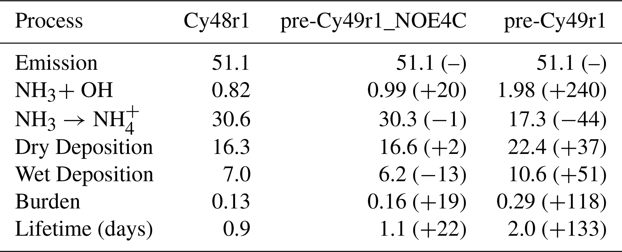
Table 4 provides the global budget terms for all three simulations, showing the significant increase in deposition terms and tropospheric burden for NH₃(g). For pre-Cy49r1, the improved gas/particle partitioning from EQSAM4Clim reduces the particle phase concentrations of the semi-volatile aerosol species which leads to an increase in the respective gas phase concentrations, also affecting aerosol pH. This determines the solubility of NH₃(g), also contributing to its reduced conversion into NH${}_{\mathrm{4}}^{+}$ (see Table 4, approx. 44 % reduction), which is an effect amplified by the inclusion of mineral cations (i.e. Ca²⁺, Na⁺, K⁺, Mg²⁺). The tropospheric lifetime of NH₃(g) more than doubles in pre-Cy49r1 allowing more transport from strong source regions, in line with changes in the tropospheric burden. Both the associated loss due to dry and wet deposition increases (37 % and 51 %, respectively), due to lower NH${}_{\mathrm{4}}^{+}$ particle production (see Sect. 4.2).

Figure 5 shows comparisons between weekly observational composites from EMEP of [NH₃(g)] against those extracted from the various IFS-COMPO simulations for 2018. The observational composite shows that there is a skewed seasonal cycle exhibiting a maximum in April/May from agricultural activity, with wintertime values being around 0.4–0.5 µg m⁻³ increasing to 0.8–1.5 µg m⁻³ during spring and summertime. This seasonal variability is captured across all simulations with a high correlation with a Pearsons's R value between 0.71–0.73. For wintertime there is limited variability and an associated low weekly bias of around 0.1 µg m⁻³. For summertime, there is a weekly bias of between 0.5–1.0 µg m⁻³ in Cy48r1 (yearly MB of approximately 0.5 µg m⁻³), with the MB almost doubling for pre-Cy49r1 (with a yearly MB of approximately 0.7 µg m⁻³.

Table 4 The tropospheric NH₃ budget in Tg N yr⁻¹ for 2018 as calculated by Cy48r1, pre-Cy49r1_NOE4C and pre-Cy49r1, with the associated percentage differences being provided in parentheses as e.g. ((pre-Cy49r1-Cy48r1)$/$Cy48r1) × 100. All global budget terms are closed.

The bottom left panel of Fig. 5 shows the corresponding comparisons of [NH${}_{\mathrm{4}}^{+}$] in Europe using the weekly observational means from the EMEP network. There is a reversed seasonality for [NH${}_{\mathrm{4}}^{+}$] with higher [NH${}_{\mathrm{4}}^{+}$] during wintertime due to the colder temperatures decreasing the volatility of the particles (e.g. Tang et al., 2021). Moreover, for Cy48r1 there is clearly a large positive bias of [NH${}_{\mathrm{4}}^{+}$] with only minor changes introduced due the wet scavenging in pre-Cy49r1_NOE4C. Wintertime biases are reduced in pre-Cy49r1 especially for weeks which exhibit peaks in the observational means which IFS-COMPO can capture.

Similar comparisons are shown for the US in the bottom right panel of Fig. 5 using weekly composites assembled from the CASTNET data. In contrast to the seasonal cycle for [NH₃(g)], which peaks during April/May, there is no corresponding seasonal cycle in the weekly [NH${}_{\mathrm{4}}^{+}$] values peaks, being consistent between 0.4–0.5 µg m⁻³ during summertime. This indicates that a saturation occurs with respect to NH${}_{\mathrm{4}}^{+}$ particle formation which is linked to availability of HNO₃(g) (cf. see Sect. 4.3. below). Again, significant biases exist in Cy48r1 and pre-Cy49r1_NOE4C, reaching around 1.0 µg m⁻³ during summertime (which is 200 % of the summertime observational values). Applying EQSAM4Clim essentially removes this positive MB in pre-Cy49r1, resulting in good agreement for the entire year.

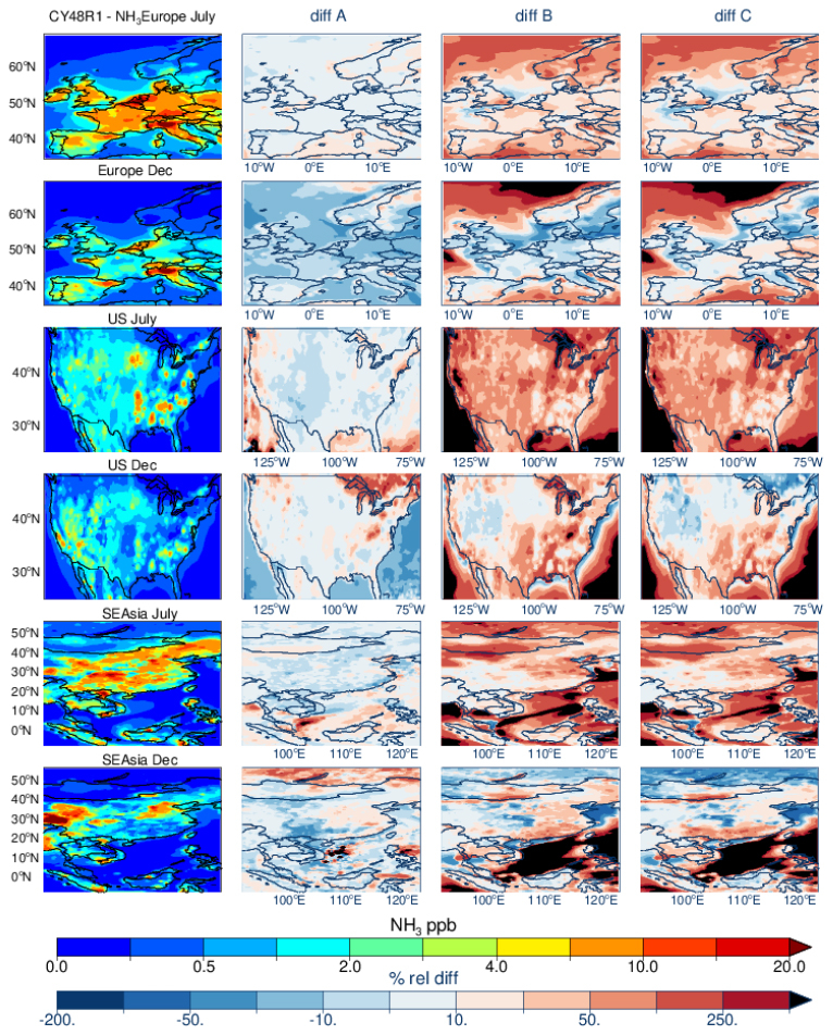
Figure 4 As for Fig. 1 except for NH₃. Panel definitions: Diff A = (pre-Cy49r1_NOEQ4C − Cy48r1)$/$Cy48r1; Diff B = (pre-Cy49r1-Cy48r1)$/$Cy48r1 and Diff C = (pre-Cy49r1-pre-Cy49r1_NOEQ4C)$/$Cy48r1.

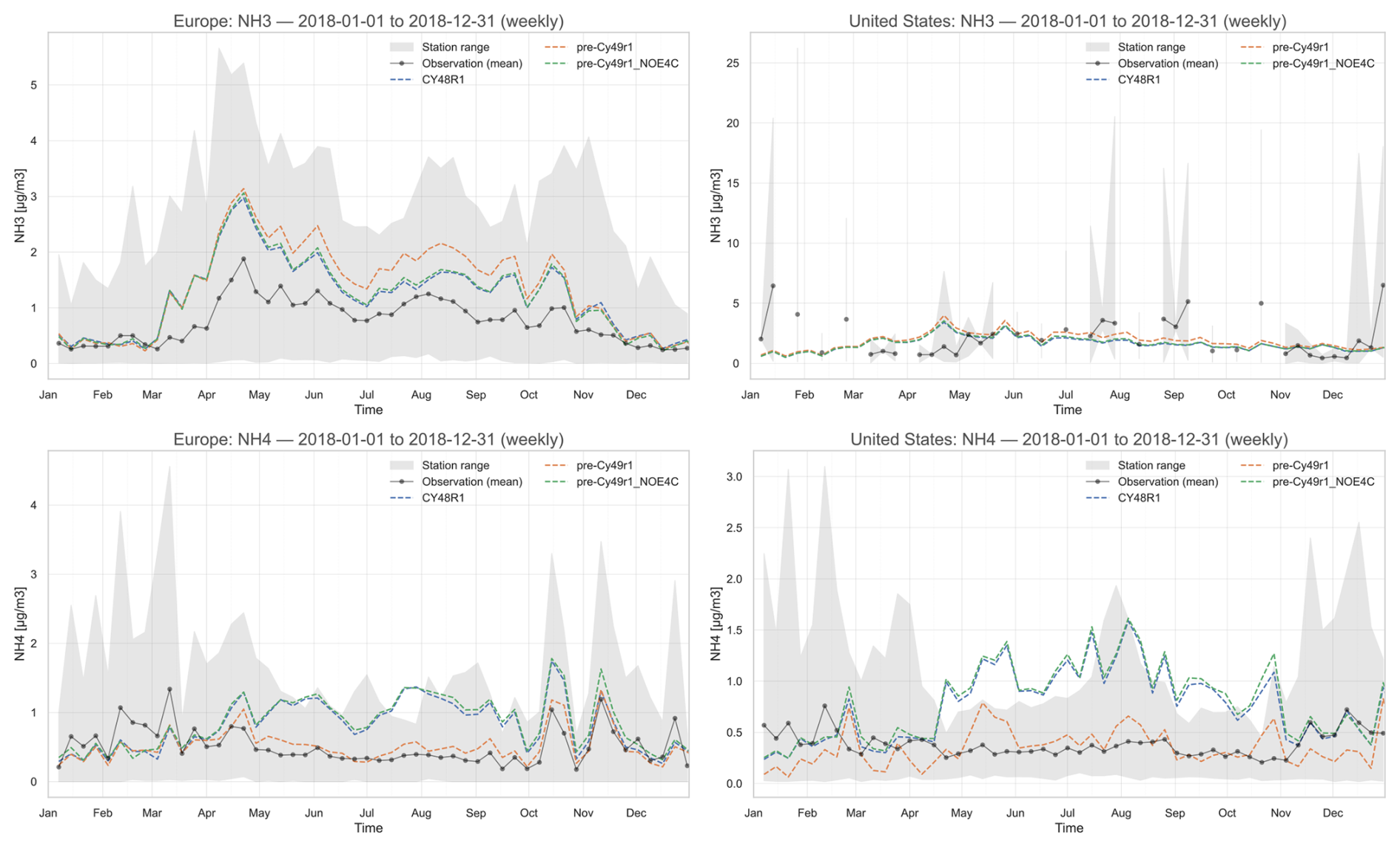
Figure 5 A comparison of weekly mean [NH₃(g)] and [NH${}_{\mathrm{4}}^{+}$] at the surface for Europe (left panels; µg m⁻³) and the US (right panels) as simulated in IFS-COMPO as compared against the composites of measurements taken from EMEP and CASTNET for 2018. For the US, the data for NH₃(g) is taken from the AMoN measurement network in the top right panel. The data frequency provided for the Southeast Asia region does not allow a corresponding plot, although yearly statistics are provided in Table 5. The grey band shows the station range (min–max) of observed weekly means at each time.

Table 5 As for Table 3 except for NH${}_{\mathrm{4}}^{+}$.

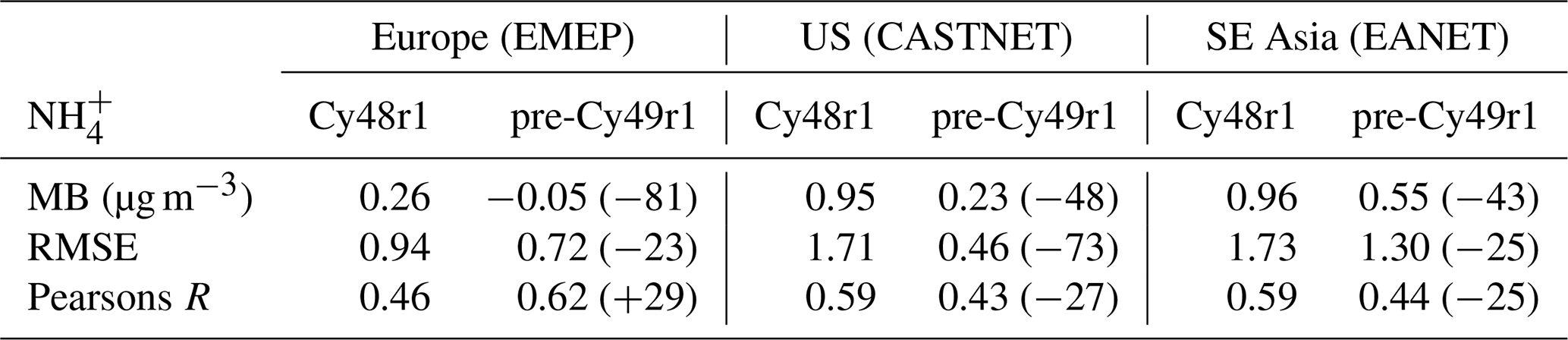
Figure 6 shows the distribution of the corresponding yearly mean [NH${}_{\mathrm{4}}^{+}$] for the three chosen regions for both Cy48r1 and pre-Cy49r1 during 2018, with the associated regional yearly mean statistics being given in Table 5. The location of the measurement sites is shown in each panel, with the respective yearly mean values within each circle. Significant decrease in the conversion rate of NH₃ in pre-Cy49r1 results in lower [NH${}_{\mathrm{4}}^{+}$]. This is a result of the improved gas/aerosol partitioning and the subsequent increase in aerosol pH when applying EQSAM4Clim (see Table 4; Rémy et al., 2024). More direct depositional loss to the surface for NH₃(g) occurs in pre-Cy49r1 due to increased residence time. There is a wide variability in the simulated aerosol pH between regions, with Europe exhibiting aerosol pH values of around 3–4, whereas the southern US and northern China exhibit aerosol pH values in the range 2–3 (Pan et al., 2024; Rémy et al., 2024) which indirectly affects the temporal variability in NH${}_{\mathrm{4}}^{+}$ production. Once formed, regional transport contributes to the continental distribution of NH${}_{\mathrm{4}}^{+}$ away from strong source regions (e.g. Simpson et al., 2010; Renner and Wolke, 2010; Du et al., 2020).

For Europe (top panels), most observational yearly mean values are between 0.2–1.2 µg m⁻³ which are exceeded by > 50 % in Cy48r1. In pre-Cy49r1 the reductions in the yearly mean [NH${}_{\mathrm{4}}^{+}$] are of the order of 0.5–1.0 µg m⁻³ and result in low yearly mean [NH${}_{\mathrm{4}}^{+}$] values for e.g. Spain/UK, whilst reducing maximal concentrations by approx. 50 % in northern Italy. This subsequently contributes to a reduction in the cumulative PM_2.5 biases for this region as shown in Rémy et al. (2024) for 2019. The associated MB values in Table 5 show a significant reduction in the bias (> 80 %) along with an increase in the correlation coefficient, although the simulated NH${}_{\mathrm{4}}^{+}$ distribution is still only moderately correlated (r=0.62). Unfortunately, the lack of available measurements means no quantification of the performance of IFS-COMPO around the mediterranean can be shown. It should be noted that with a more realistic distribution and seasonal variability in NH₃(g) emissions (e.g. Shephard et al., 2011; Dammers et al., 2019), the [NH${}_{\mathrm{4}}^{+}$] distributions shown here will not be affected as other SIA species determine the NH₃ – NH${}_{\mathrm{4}}^{+}$ gas/aerosol partitioning.

For the US (middle panels) similar decreases in yearly mean [NH${}_{\mathrm{4}}^{+}$] values occur in pre-Cy49r1 as compared to Cy48r1, with very low concentrations of between 0.1–0.4 µg m⁻³ for the west of the US, which shows less bias when compared against the observational mean values. This causes a reduction in the yearly mean regional bias of around 0.7 µg m⁻³ as shown in Table 5. A gradient exists in the aerosol pH from EQSAM4Clim ranging from yearly mean values of pH = 3.0 towards the northwest of the US and becoming more acidic towards the southwest US with yearly mean values of pH = 2.0 (Rémy et al., 2024). This reduces the transfer of NH₃(g), thus moderating NH${}_{\mathrm{4}}^{+}$ production (cf. Table 5). For the northeast of the US with high NO_x emissions, there are reductions of between 0.5–1.0 µg m⁻³. For the South-western US, with high [NH₃(g)] from agriculture (cf. Fig. 5) there are reductions of between 0.3–1.0 µg m⁻³. There is a degradation in the correlation coefficient exhibiting a moderate yearly mean correlation with significant overestimates for the South-western US as shown for the comparisons of [NH₃(g)] at selected sites in Fig. 5.

For Southeast Asia (bottom panels), the simulated yearly mean [NH${}_{\mathrm{4}}^{+}$] over land are typically much higher than those simulated for either Europe or the US, with maximal values of between 7.0–9.0 µg m⁻³ for eastern China, in-spite of the similar surface mixing ratios in NH₃(g) between Europe and China as shown in Fig. 5. This difference is predominantly driven by the relatively high HNO₃(g) in China due to the more polluted chemical regime (the availability of O₃(g), NO₂(g) and OH(g) determining gas-phase HNO₃(g) production). Applying EQSAM4Clim in pre-Cy49r1 results in significant decreases of between 1–2 µg m⁻³ [NH${}_{\mathrm{4}}^{+}$] as associated with the highest yearly mean [NH${}_{\mathrm{4}}^{+}$] > 6.0 µg m⁻³. This reduces the associated yearly mean regional bias by 0.4 µg m⁻³, with a corresponding reduction in the correlation, due to less transport. Again, the lack of sampling sites in the region with high primary NH₃(g) emissions skews the associated yearly mean biases. For the more remote locations (e.g. Mongolia/South China Sea) low values of < 0.5 µg m⁻³ are captured well in both Cy48r1 and pre-Cy49r1.

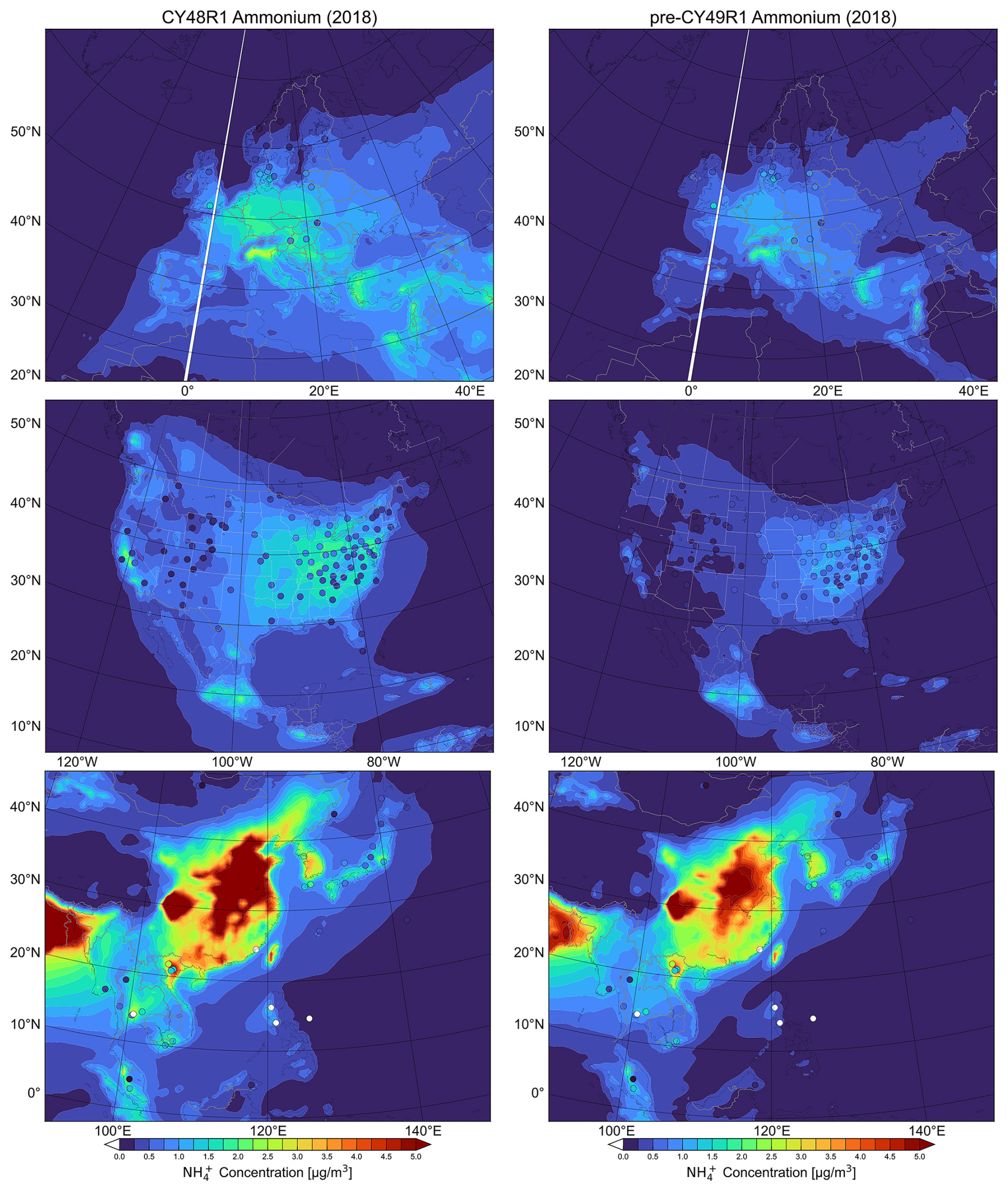
Figure 6 Comparisons of yearly mean [NH${}_{\mathrm{4}}^{+}$] simulated at the surface in Cy48r1 and pre-Cy49r1 when compared against measurements for the three selected regions during 2018 (µg m⁻³). The corresponding regional statistics are provided in Table 5. Site locations and observed values, taken from the EMEP, CASTNET and EANET networks respectively, are shown in circles.

4.3 HNO₃ and NO${}_{\mathrm{3}}^{-}$

Figure 7 shows the monthly mean distributions and mixing ratios of HNO₃(g) for July and December 2018 for the three chosen global regions for Cy48r1, along with the relative differences when compared with pre-Cy49r1_NOE4C and pre-Cy49r1. The corresponding global chemical budget terms for HNO₃(g) during 2018 are provided in Table 6. No direct emission of HNO₃ occurs in IFS-COMPO, which is often prescribed in global chemistry transport models to represent e.g. chemistry in the plumes of ships (e.g. Vinken et al., 2011), with the main source being the oxidation of NO₂ by OH in the gas-phase as shown in Table 6. This production term increases in pre-Cy49r1 by approx. 14 % because of the enhancements in OH via changes in O₃ (not shown). For heterogeneous conversion, the cumulative HNO₃ production term is approximately 50 % that of the gas-phase production term, remaining relatively constant between simulations. There is a shift between fine mode NO${}_{\mathrm{3}}^{-}$ (NH₄NO₃) and coarse mode NO${}_{\mathrm{3}}^{-}$ (CaNO₃ $/$ NaNO₃), strengthening the link between NH${}_{\mathrm{4}}^{+}$ and NO${}_{\mathrm{3}}^{-}$ in pre-Cy49r1. Both dry and wet loss terms increase significantly due to the increase in the availability of HNO₃(g), which reduces the fraction converted to NO${}_{\mathrm{3}}^{-}$. The temporal variability of HNO₃(g) is influenced by the magnitude and extent of regional NO_x emissions, photochemical activity (via OH formation), gas/aerosol partitioning (where particles with high SO${}_{\mathrm{4}}^{=}$ content having an associated low NO${}_{\mathrm{3}}^{-}$ content) and scavenging in clouds and aerosols.

For Europe very low surface mixing ratios occur over land for both months shown in Cy48r1 (< 0.1 ppb), which is surprising considering that the Benelux has been shown to have high NO_x levels (van der A, 2024) therefore likely to have correspondingly high HNO₃(g) mixing ratios. Higher mixing ratios of between 0.25–0.5 ppb occur around the Coasts and the Mediterranean originating from direct shipping emissions of NO₂. This can lead to elevated NO${}_{\mathrm{3}}^{-}$ concentration due to uptake of HNO₃(g) on sea salt, which might be too high as the current formulation of EQSAM4Clim only assumes thermodynamic equilibrium which is not dynamically limited. Here, an aerosol dynamical model refers to a microphysical framework that prognoses particle number/size distributions (via condensational growth, coagulation, nucleation and inter-mode transfer), thus enabling kinetically limited gas-to-particle uptake and condensation processes beyond the instantaneous thermodynamic equilibrium assumed by EQSAM4Clim (Metzger et al., 2018). A coupling with a dynamical aerosol model is foreseen for future versions of IFS-COMPO. In contrast, the application of EQSAM4Clim in pre-Cy49r1 results in large increases in surface HNO₃(g) at continental scale during July. For December, the relative differences in pre-Cy49R1 compared to Cy48r1 show increases in HNO₃(g) at latitudes below 60° N, together with decreases of between 25 %–75 % at latitudes higher than 60° N, i.e. at lower temperatures, and under a relatively low NO_x environment.

For the US, the highest HNO₃(g) mixing ratios in Cy48r1 occur for the eastern states and California (1–2 ppb), with much lower values in the more remote central US (0.1–0.2 ppb), with a strong seasonal cycle in maximal values peaking in July. Comparing relative differences between simulations shows a significant increase of surface HNO₃(g) in pre-Cy49r1 (between 0.1–6 ppb) at continental scale for both months, with the largest increases occurring in the northern States. In contrast to Europe no significant decreases in [HNO₃(g)] occur for any location or season.

Finally, in comparison to the other regions the surface [HNO₃(g)] are highest for Southeast Asia. Maximal mixing ratios of 4–5 ppb occur towards the eastern coast (July) and central regions (cf. December). Comparing the relative differences between simulations shows significant increases of between 50 %–5000 %, apart from the more remote regions to the north where NO_x emissions are lower. As for Europe, a strong seasonality can be seen with decreases above 30° N occurring regardless of the NO_x regime. As shown for NH₃ (cf. Fig. 4), there are significant increases in HNO₃ over the ocean for both months shown, associated with lower [NO${}_{\mathrm{3}}^{-}$] (as shown by the cumulative reduction in global conversion by 50 %).

Figure 8 shows the resulting changes in surface [HNO₃(g)] across simulations for Europe when compared against weekly means from the EMEP measurement sites (top left panel). The location of these sites is shown in Fig. A1 in the Appendix, where the location of the sampling sites results in a significant bias in the evaluation towards northern Europe. No obvious seasonal cycle is evident in the observational weekly means, with concentrations in the range of 0.3–0.7 µg m⁻³, although many sites are located away from strong NO_x sources. Both Cy48r1 and pre-Cy49r1_NOE4C exhibit negative weekly biases resulting in under-estimations of around 100 % in concentrations during the summertime, although the weekly variability is captured to a degree. There is a reduction in the bias of around 0.2–0.4 µg m⁻³ in pre-Cy49r1_NOE4C due to changes in the gas-phase production term. (cf. Table 8). For pre-Cy49r1 there is a significant excess of [HNO₃(g)] due to enhanced production and less transfer into the particulate phase, despite an increase in the cumulative deposition terms. Such changes are associated with relatively low [HNO₃(g)] IFS-COMPO values of around < 0.1 ppb.

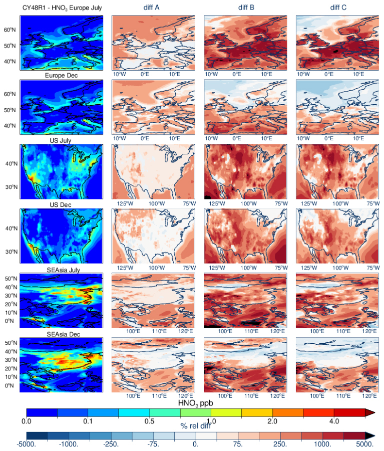
Figure 7 As for Fig. 1 except for HNO₃. Panel definitions: Diff A = (pre-Cy49r1_NOEQ4C − Cy48r1)$/$Cy48r1; Diff B = (pre-Cy49r1-Cy48r1)/Cy48r1 and Diff C = (pre-Cy49r1-pre-Cy49r1_NOEQ4C)$/$Cy48r1.

Figure 8 also shows comparisons of weekly [HNO₃(g)] from the CASTNET measurement network in the US (top right panel). As for Europe, both the concentrations and seasonal variability in the observations is low, with typical weekly concentrations being approximately 0.5 µg m⁻³. The homogeneous distribution of measurement sites in the US means the evaluation presented does not have any significant regional bias. That the observed weekly mean concentrations are rather constant is surprising considering that variability in the gas-phase chemical production term involves OH. However, changes in RH, temperature and NH₃(g) across seasons also contribute to the seasonal lifetime. In contrast to Europe, both Cy48r1 and pre-Cy49r1_NOE4C show good agreement against the measurements with weekly biases of the order of 0.2–0.25 µg m⁻³. However, for pre-Cy49r1 a large positive bias is introduced directly from the use of EQSAM4Clim due to a limitation in the ability for HNO₃ to condense on particle surfaces. This means that condensed HNO₃ does not contribute to NH₄NO₃ formation (which requires a coupling of EQSAM4Clim with an aerosol dynamical model) as proposed for future cycles of IFS-COMPO. It also shows that although the cumulative global dry and wet deposition terms in pre-Cy49r1 have increased markedly compared to Cy48r1 (cf. Table 6), fluxes are not large enough to compensate for the reduced aerosol formation.

Table 6 The tropospheric HNO₃ budget in Tg N yr⁻¹ for 2018 as calculated by Cy48r1, pre-Cy49r1_NOE4C and pre-Cy49r1, with the associated percentage differences being provided in parentheses as e.g. ((pre-Cy49r1-Cy48r1)$/$Cy48r1) × 100. All global budget terms are closed.

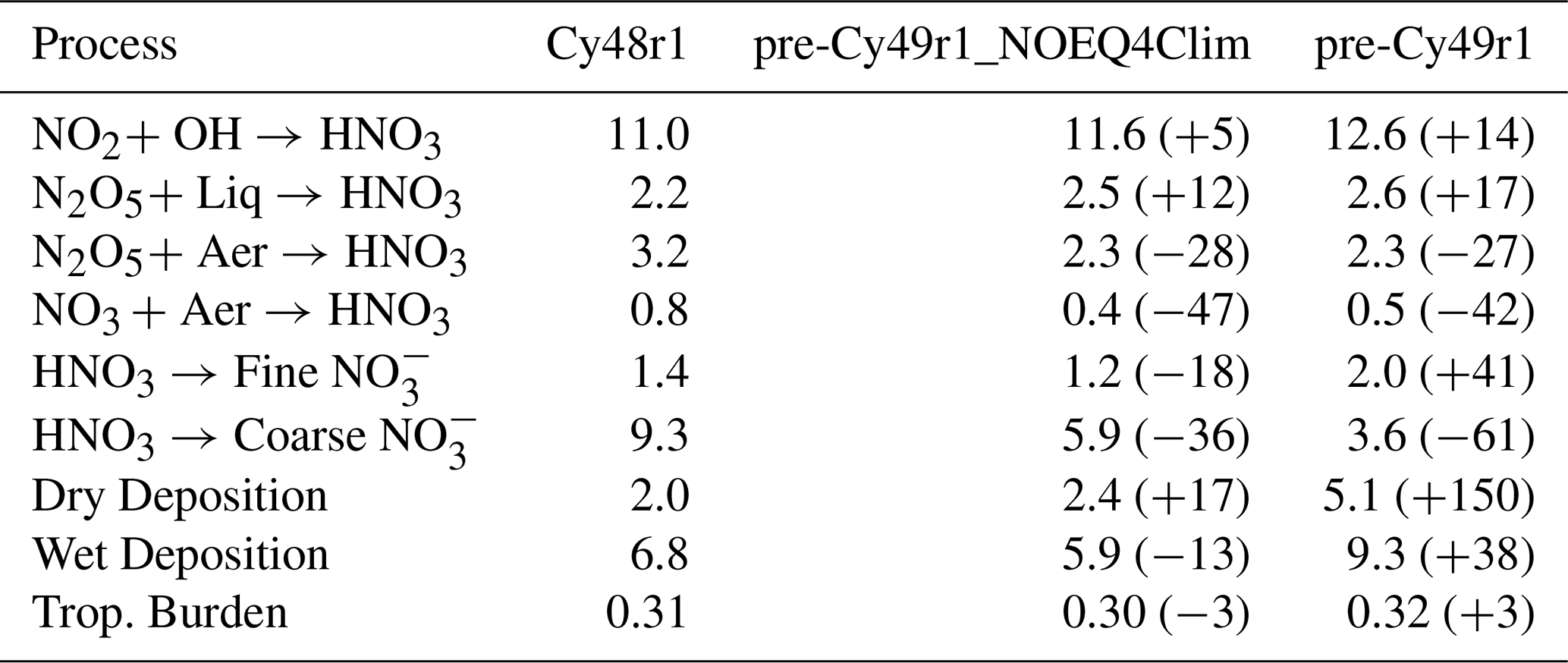
Figure 8 also shows the corresponding changes in surface [NO${}_{\mathrm{3}}^{-}$] for Europe (bottom left panel). The observational composites show that [NO${}_{\mathrm{3}}^{-}$] has concentrations almost twice those of the corresponding [HNO₃(g)] during wintertime. For summertime there is almost an equal split in the phase partitioning between precursor and SIA. Unlike for HNO₃(g), a shallow concave seasonal cycle exists in the weekly observational composites, related to seasonal differences in temperatures and lifetime (Tang et al., 2021). Both Cy48r1 and pre-Cy49r1_NOE4C fail to capture the correct seasonality and exhibit higher concentrations during summertime, resulting in substantial positive biases of 1–2 µg m⁻³. Considering the associated biases in [HNO₃(g)] shows that the HNO₃-NO${}_{\mathrm{3}}^{-}$ partitioning is not captured well. For pre-Cy49r1 the description of the seasonal cycle is significantly improved due to the inclusion of EQSAM4Clim, resulting in much lower biases of < 0.5 µg m⁻³ throughout the year, also pointing to the importance of a better representation of gas/particle partitioning. The corresponding changes in [NO${}_{\mathrm{3}}^{-}$] in the simulations are evaluated against weekly composites from the CASTNET measurement network are shown in the bottom right panel of Fig. 8. A similar seasonal cycle exists as for Europe with similar concentrations. For Cy48r1 and pre-Cy49r1_NOE4C an inverse seasonal variability occurs in [NO${}_{\mathrm{3}}^{-}$] as compared with the observational weekly means, resulting in significant positive biases of around 1.0–1.5 µg m⁻³. For pre-Cy49r1 biases decrease by an order of magnitude and the seasonal variability is improved markedly, again showing improved particle distribution when using EQSAM4Clim.

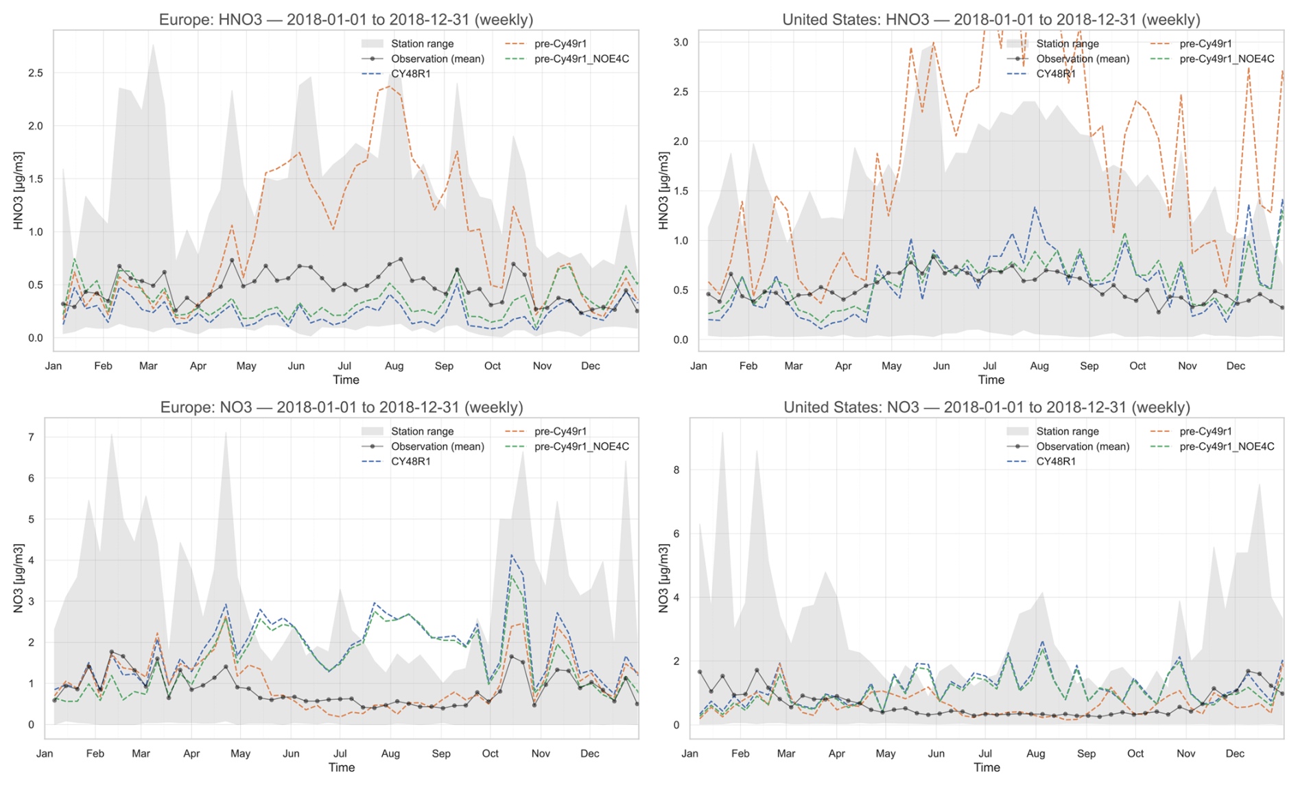
Figure 8 A comparison of weekly mean [HNO₃(g)] and [NO${}_{\mathrm{3}}^{-}$] for Europe (left panels; µg m⁻³) and the US (right panels) at the surface as simulated in IFS-COMPO as compared against measurement composites from EBAS (left) and CASTNET (right) stations for 2018. The grey band shows the station range (min–max) of observed weekly means at each time.

In Fig. 9 we show the corresponding regional distributions of the yearly mean [NO${}_{\mathrm{3}}^{-}$] for Cy48r1 and pre-Cy49r1 during 2018 for the three chosen global regions, where the associated changes in the regional yearly mean statistics are provided in Table 7. Some commonality exists between the changes shown for yearly mean [NH${}_{\mathrm{4}}^{+}$] and yearly mean [NO${}_{\mathrm{3}}^{-}$], due to the speciation of the SIA involved. The cumulative sums of the smaller NO${}_{\mathrm{3}}^{-}$ particle (fine mode NO${}_{\mathrm{3}}^{-}$ in Table 6 with the form NH₄(NO₃)) and the larger NO${}_{\mathrm{3}}^{-}$ particle (coarse mode NO${}_{\mathrm{3}}^{-}$ in Table 6 with the form of CaNO₃ and NaNO₃) are both included in the plots. Therefore, the changes evaluated here are a combination of changes to both the fine and coarse mode NO${}_{\mathrm{3}}^{-}$, rather than the changes associated with individual particle sizes. In contrast to the reduced N analysis provided above, which is impacted more directly due to changes in the fine mode NO${}_{\mathrm{3}}^{-}$, with [NO${}_{\mathrm{3}}^{-}$] also indirectly affected by the coarse mode assumptions through the effect of cations on the neutralisation level that subsequently controls the gas/aerosol equilibrium partitioning. The change in the partitioning for HNO₃ shown above results in an associated reduction in the fraction of NO_x held in particulate form due to e.g. a higher dry deposition component.

For Europe, the simulated yearly mean [NO${}_{\mathrm{3}}^{-}$] in Cy48r1 generally ranges between 0.2–2.0 µg m⁻³ over Scandinavia/Spain and the surrounding seas and between 2.0–6.3 µg m⁻³ over northwestern/central Europe and the Mediterranean, becoming lower towards the northeast and southwest. The highest European NO_x emissions occur around the south-east of the UK, Benelux, the Ruhr, and Po valleys (e.g. Liu et al., 2021; van der A., 2024). This, and the rather homogeneous distribution within central Europe shows that a significant degree of transport occurs once NO${}_{\mathrm{3}}^{-}$ particles are formed. No such continental gradient in the yearly mean [NO${}_{\mathrm{3}}^{-}$] exists in the observational mean values indicating an overestimate in IFS-COMPO. Nevertheless, in pre-Cy49r1 decreases in [NO${}_{\mathrm{3}}^{-}$] of between 2–4 µg m⁻³ occur for the Baltic states/France/Germany and over the Mediterranean Sea (from relatively high shipping NO_x emissions) compared to Cy48r1. This results in much better agreement with the yearly mean observed values for the individual measurement stations. The yearly regional MB is reduced by ≅ 90 %, decreasing to 0.1 µg m⁻³ in pre-Cy49r1 with an associated increase in the correlation coefficient due to lower transport of [NO${}_{\mathrm{3}}^{-}$] out of the main source region. A large impact occurs due to the acidification of sea salt aerosols under high NO_x emission from dense shipping lanes, which can be seen by similar [NO${}_{\mathrm{3}}^{-}$] reductions over the sea, though difficult to evaluate due to the lack of sufficient in-situ measurements.

For the US, there is a similar impact on [NO${}_{\mathrm{3}}^{-}$] as shown for Europe, where the high yearly MB in [NO${}_{\mathrm{3}}^{-}$] decreases significantly (94 %) from Cy48r1 to pre-Cy49r1 (bottom right panel of Fig. 8). For Cy48r1, [NO${}_{\mathrm{3}}^{-}$] typically ranges between 2–4 µg m⁻³ with medium-range transport resulting in appreciable concentrations over the surrounding oceans. There is surprisingly little variability in the observed yearly mean [NO${}_{\mathrm{3}}^{-}$] despite the large difference in the resident [HNO₃(g)] across different states of the US related to the distribution of the NO_x emissions (Fig. 7; Goldberg et al., 2021). Only in the southwest, around California, the yearly mean [NO${}_{\mathrm{3}}^{-}$] > 2.0 µg m⁻³, shows typical yearly mean [NO${}_{\mathrm{3}}^{-}$] being ≤ 1.0 µg m⁻³ in pre-Cy49r1 for most of the US. This implies that the cations used as input for EQSAM4Clim imposes a limit concerning the phase-transfer of HNO₃(g) into more acidic aerosols via neutralisation of the anions by cations in the particle phase.

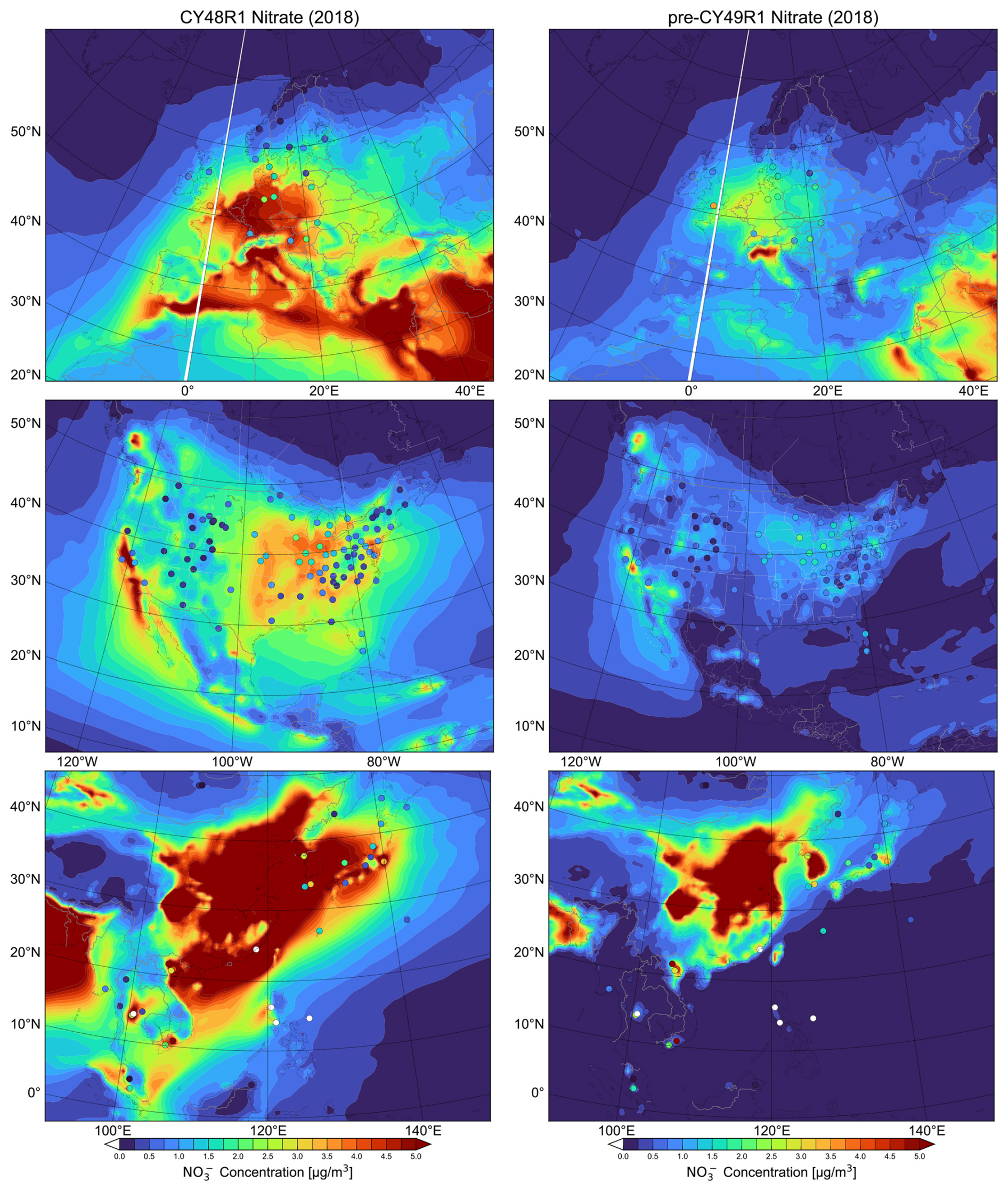
Figure 9 Comparisons surface comparisons of [NO${}_{\mathrm{3}}^{-}$] simulated in Cy48r1 and pre-Cy49r1 as compared against measurements for the three selected regions given in µg m⁻³. The corresponding regional statistics are provided in Table 7. Site locations and observed values, taken from the EMEP, CASTNET and EANET networks respectively, are shown in circles.

Table 7 As for Table 3 except for NO${}_{\mathrm{3}}^{-}$.

5 The changes in regional wet deposition

In this section, we evaluate the temporal distribution and biases associated with the yearly wet deposition terms of soluble trace gas species and particulates. All three SIA are lost to the surface by both dry and wet deposition processes. Over the last decades the main source of acidification has shifted from SO_x based to NO_x based in line with the reduction measures imposed for SO_x and the increase and associated emission changes from e.g. road transport. Here we evaluate whether pre-Cy49r1 captures the correct wet scavenging and improves on the performance of Cy48r1 for the various dissolved precursors and SIA. Evaluations are made using comparisons of model output against yearly wet deposition totals as taken from the observational networks introduced in Sect. 3. The concentrations of the dissolved precursors (i.e. SO₂(aq), NH₃(aq) and HNO₃(aq)) also undergo wet deposition (in IFS-COMPO) and cannot be differentiated well in the observational networks and are therefore included in the measured totals. The wet deposition term is also influenced by meteorological parameters such as the simulated large-scale and convective mixing, liquid and solid precipitation droplet size, SAD, and the frequency and intensity of precipitation as provided by the IFS model.

The changes in the global tropospheric burden, lifetime, dry and wet deposition totals for SO${}_{\mathrm{4}}^{\mathrm{2}-}$, NH${}_{\mathrm{4}}^{+}$, NO${}_{\mathrm{3}}^{-}$ (fine) and NO${}_{\mathrm{3}}^{-}$ (coarse) during 2018 are given in Table 8. The corresponding statistics for the changes in wet deposition between Cy48r1 and pre-Cy49r1 as compared against yearly observational means yearly for SO_x, reduced N and oxidised N are provided for the three chosen global regions in Table 9.

Table 8 The global budget values for the burden, tropospheric lifetime, wet and dry deposition terms for SO${}_{\mathrm{4}}^{\mathrm{2}-}$, NH${}_{\mathrm{4}}^{+}$ and NO${}_{\mathrm{3}}^{-}$ for 2018. Totals are provided in Tg S yr⁻¹ and Tg N yr⁻¹. Percentage difference changes are calculated as ((pre-Cy49r1-Cy48r1)$/$Cy48r1) × 100 and given in parentheses.

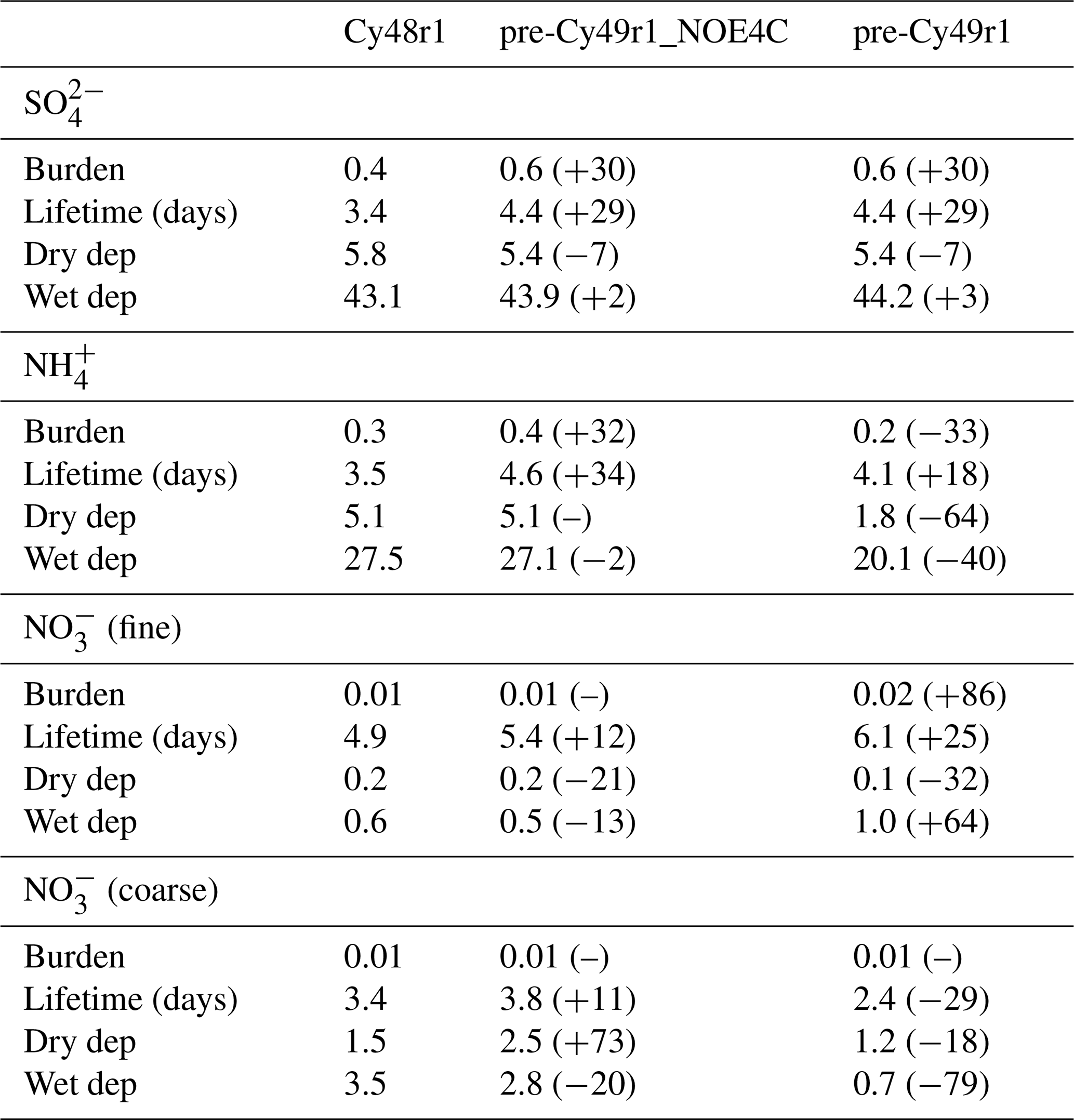
Table 9 The yearly MB, RMSE and Pearsons R values for the comparisons of the yearly mean regional wet deposition totals of dissolved SO₂+SO${}_{\mathrm{4}}^{=}$, NH₃+NH${}_{\mathrm{4}}^{+}$ and HNO₃+NO${}_{\mathrm{3}}^{-}$ as compared against composites assembled from the regional observation networks for 2018 shown in Figs. 9–11 for Europe, the US and Southeast Asia. Percentage difference changes are calculated as ((pre-cy49r1-Cy48r1)$/$Cy48r1) × 100 and given in parentheses.

5.1 Total yearly wet S deposition

Figure 10 shows the regional distribution and values of yearly wet S deposition for Europe, the US, and Southeast Asia in both Cy48r1 and pre-Cy49r1 during 2018. To allow a direct comparison across regions we use a colour scale which covers values larger than 500 mgS m⁻² yr⁻¹ in Southeast Asia. The global budget terms for SO${}_{\mathrm{4}}^{\mathrm{2}-}$ are presented in Table 8 and show that, despite the global burden increasing by one third, only very small increases of a few percent occur in the yearly wet SO${}_{\mathrm{4}}^{\mathrm{2}-}$ totals (Rémy et al., 2024), with associated decreases in the dry deposition term. The significant increase in the tropospheric SO${}_{\mathrm{4}}^{\mathrm{2}-}$ lifetime means more remains in the aerosol phase and will increase both AOD and the degree of scattering in IFS-COMPO as shown for AOD comparisons in Rémy et al. (2024). The most significant change is in the direct gas-phase production term of H₂SO₄(g), where increases in [SO₂(g)] subsequently increase the total mass scavenged into aqueous cloud droplets. This results in an extent of acidification (slowing in-situ oxidation; cf. Table 2), which is buffered by the increased phase transfer of NH₃(g) (cf. Table 4). These changes are the result of updates to the scavenging approach rather than the application of EQSAM4Clim. Although there is a 16 % reduction in the total global SO₂(aq) wet deposition (cf. Table 2), this is compensated for by increases in [SO${}_{\mathrm{4}}^{\mathrm{2}-}$(aq)] which results in an increase in the cumulative wet S deposition yearly totals.

For Europe (top panels), the changes between model simulations are like the changes in the SO₂(g) and SO${}_{\mathrm{4}}^{\mathrm{2}-}$ particle concentrations discussed in Sect. 4. Compared against the yearly mean observational values from EMEP, which range from 100–500 mgS m⁻² yr⁻¹, there is an underestimation in Cy48r1 of approximately 100 mgS m⁻² yr⁻¹ for northwest Europe. For the observational means in Ireland, Poland, northern Spain and on the Iberian Peninsula negative MB are enhanced to around 300 mgS m⁻² yr⁻¹. This indicates missing local source terms in the global emission inventory provided as monthly mean fluxes. For other regions, the agreement is satisfactory capturing the observed deposition gradient from Germany into Austria/northern Italy. For pre-Cy49r1, strong similarity exists for Benelux, Denmark, and Italy, where negative biases of around 50–100 mgS m⁻² yr⁻¹ occur. A significant negative yearly MB exists in Europe, which decreases by around 10 % in pre-Cy49r1 (cf. Table 9) with a marginal increase in the correlation. Considering the associated positive MB for aerosol SO${}_{\mathrm{4}}^{\mathrm{2}-}$ shown during summertime (cf. Fig. 2), there is an indication that not enough phase transfer occurs, thus negative MB values for the yearly deposition totals, and the large observational means at selected stations influencing the regional yearly mean.

For the US (middle panels) there is a stark contrast to the changes shown for Europe. Analysis of the yearly observational yearly mean values from CASTNET shows that a gradient exists in the wet deposition yearly totals from east to west, similar to that for SO₂(g) and the location of primary SO₂ emission sources (cf. Fig. 1). Maximal values of 300–400 mgS m⁻² yr⁻¹ occur towards the east coast where a positive MB occurs for [SO${}_{\mathrm{4}}^{\mathrm{2}-}$] (cf. Fig. 3). For Cy48r1, this gradient in yearly wet deposition is captured to a large degree, albeit with significant positive biases of > 100 mgS m⁻² yr⁻¹ with a maximal range of 700–900 mgS m⁻² yr⁻¹. There is a significant yearly wet deposition of SO_x in the Atlantic (250–400 mgS m⁻² yr⁻¹) due to the local oxidation of DMS (released from the ocean) and the long-range transport of SO₂(g) $/$ SO${}_{\mathrm{4}}^{\mathrm{2}-}$ from the anthropogenic source regions. In pre-Cy49r1 the area of maximal wet S deposition increases around, e.g., New York state extending south to Texas resulting in an increase in the positive yearly MB for the US by nearly 40 % (to 190 mgS m⁻² yr⁻¹). This contrasts with the significant improvement in the yearly MB for [SO${}_{\mathrm{4}}^{\mathrm{2}-}$] given in Table 3, which provides the continental mean rather than statistics for the east coast. The changes are determined by changes in the scavenging of SO${}_{\mathrm{4}}^{\mathrm{2}-}$ particles into the aqueous phase, with the application of EQSAM4Clim having a minor influence (Table 8).

Finally for Southeast Asia (bottom panels), the magnitude of EANET yearly wet depositional totals show that more than twice the amount of S deposition occurs as measured in either Europe or the US over an identical period and a much wider area, reaching 1200–1300 mgS m⁻² yr⁻¹ in central and eastern China (not shown). The spatial distribution of stations shows that a negative gradient exists between deposition totals in China and those extending towards Myanmar (west) and Japan (east) (2000–2200 mgS m⁻² yr⁻¹; not shown). This indicates the importance of the transport component of SO${}_{\mathrm{4}}^{\mathrm{2}-}$ when considering the low regional SO₂(g) precursor mixing ratios around the equator (cf. Fig. 1), and that the primary sources are typically infrequent volcanic eruptions for the region between 5° N–5° S (Fioletov et al., 2020) that typically inject the SO₂ above the boundary layer (thus with a limited impact on the surface values). Towards the coast of eastern China and Japan, the observations show yearly totals of 250–350 mgS m⁻² yr⁻¹, in contrast to high values near the middle of China. Such local scale variability is not captured using the current emission inventory that is employed, where the positive MB increases significantly in pre-Cy49r1 using the same observational stations and emission estimates (cf. Table 3). The extent of high wet deposition values reaches hundreds of kilometres from the coast far away from prescribed emission sources. The regional yearly MB improves markedly to 8.7 mgS m⁻² yr⁻¹ in pre-Cy49r1 despite increases in the MB and decreases in the Pearson's R value for [SO${}_{\mathrm{4}}^{\mathrm{2}-}$] (Table 3).

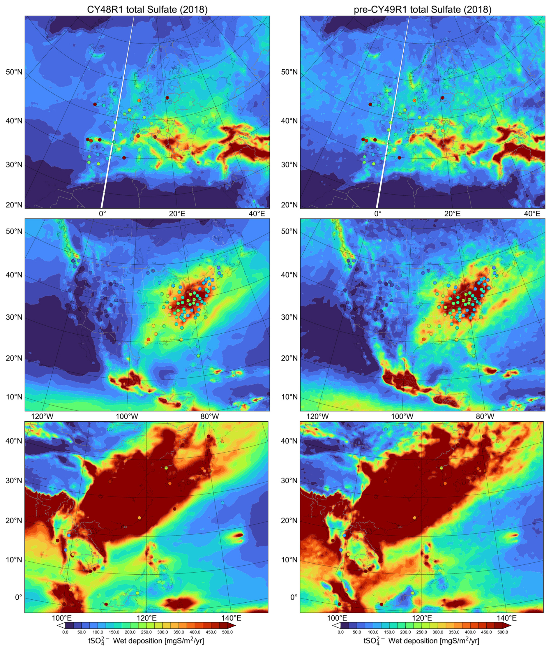
Figure 10 Yearly comparisons of the cumulative wet deposition totals of dissolved SO₂ and SO${}_{\mathrm{4}}^{\mathrm{2}-}$ aerosol (mgS m⁻² yr⁻¹) for 2018 as simulated in Cy48r1 (left column) and pre-Cy49r1 (right column) shown for Europe (top), the US (middle) and Southeast Asia (bottom). The corresponding statistics are provided in Table 9. Site locations and observed values, taken from the EMEP, CASTNET and EANET networks respectively, are shown in circles.

5.2 Total yearly wet NH_x deposition

In Fig. 11 we show the corresponding changes in the total yearly mean wet deposition of reduced N for both Cy48r1 and pre-Cy49r1 during 2018 for the three global regions. The location of the sampling stations is identical to those shown above for the wet S deposition evaluation. In Table 8, the global chemical budget terms for NH${}_{\mathrm{4}}^{+}$ show that for pre-Cy49r1_NOE4C there is an increase the tropospheric burden by one third (as for SO${}_{\mathrm{4}}^{\mathrm{2}-}$, with (NH₄)₂SO₄ being a dominant SIA, Seinfeld and Pandis, 2006). This is subsequently reversed when applying EQSAM4Clim in pre-Cy49r1 This results in significant decreases in both the total yearly global dry and wet deposition terms for reduced N (> 50 % from Table 8).

For Europe (top panels), where high summertime NH₃(g) mixing ratios are simulated (cf. Fig. 4 in Sect. 4), the EMEP observational yearly wet deposition totals show that peak values exist in the Balkans, Germany, Austria and northern Italy (Po valley), and that local regional variability exists in e.g. France (ranging between 250–350 mgN m⁻² yr⁻¹). For regions with low NH₃ emissions, such as Scandinavia and the Iberian Peninsula, wet deposition totals generally have a lower range, of between 50–200 mgN m⁻² yr⁻¹. For Cy48r1, the high resident surface mixing ratios of NH₃(g) (5–15 ppb; Fig. 1) results in a relatively high NH_x yearly total wet deposition values of between 350–500 mgN m⁻² yr⁻¹ for northwest and central Europe at a country-wide scale (e.g. the Netherlands and Belgium). Measured yearly mean values from EMEP are typically exceeded, which results in a yearly MB of 61 mgN m⁻² yr⁻¹ in Cy48r1, albeit with a high correlation of 0.69 (cf. Table 8), reflecting the positive local MB shown for [NH${}_{\mathrm{4}}^{+}$] shown in Fig. 6. Comparing the yearly mean temporal distribution simulated in pre-Cy49r1 shows a significant reduction in the area with maximal values (> 450 mgN m⁻² yr⁻¹), being limited to northern Italy only. The reduction in [NH${}_{\mathrm{4}}^{+}$] (cf. Table 4) reduces the yearly MB in wet deposition by nearly 60 %, without any notable degradation in the correlation coefficient. Thus, the application of EQSAM4Clim significantly improves the simulation of reduced N wet deposition in IFS-COMPO for Europe.

For the US (middle panels), the AMoN observations show that there is a similar east-west gradient in the total reduced N wet deposition totals as that for NH₃(g) surface mixing ratios and [NH${}_{\mathrm{4}}^{+}$] distributions (cf. Figs. 4 and 6, respectively). The range in observed total wet deposition values is between 30–400 mgN m⁻² yr⁻¹ showing that, in the absence of local NH₃ emission sources, that levels of deposition are low (lower than that observed for Europe). Comparing the temporal distribution of reduced N wet deposition in Cy48r1 shows that the continental gradient is captured, although maximal values which occur towards central US are not seen in the measurements (> 100 % MB) being influenced by the high local NH₃ emission flux. For the east coast, where most primary NH₃ sources are located, there is generally an overestimation in the wet deposition simulated in Cy48r1. Compared to Europe, the yearly MB for the US is low at 9 mgN m⁻² yr⁻¹ in Cy48r1. This is a result of the large positive MB towards the east being moderated by negative in other parts of the US. There is an improvement in the MB in pre-Cy49r1, albeit with a degradation in the Pearsons' R to 0.72.

For Southeast Asia, the EANET observational yearly mean wet deposition totals show that, similar to that shown for S deposition, much higher values occur than for the other two regions presented. The yearly deposition values range between 200–2400 mgN m⁻² yr⁻¹ (not shown), with the highest measured values occurring more inland and away from coastal regions. The simulated temporal distribution in wet reduced N deposition does capture the variability across individual stations quite well across a wide area (cf. from China to Japan). In Cy48r1, the yearly MB is 12 mgN m⁻² yr⁻¹ on high yearly totals resulting in it being the lowest for all the regions, with a high correlation coefficient of 0.75. For pre-Cy49r1, there is a larger negative MB (although still relatively small compared to the large totals), in-spite of the lower (positive) MB simulated for the [NH${}_{\mathrm{4}}^{+}$] comparisons as compared to Cy48r1 (cf. Table 5), again with a modest degradation in the correlation.

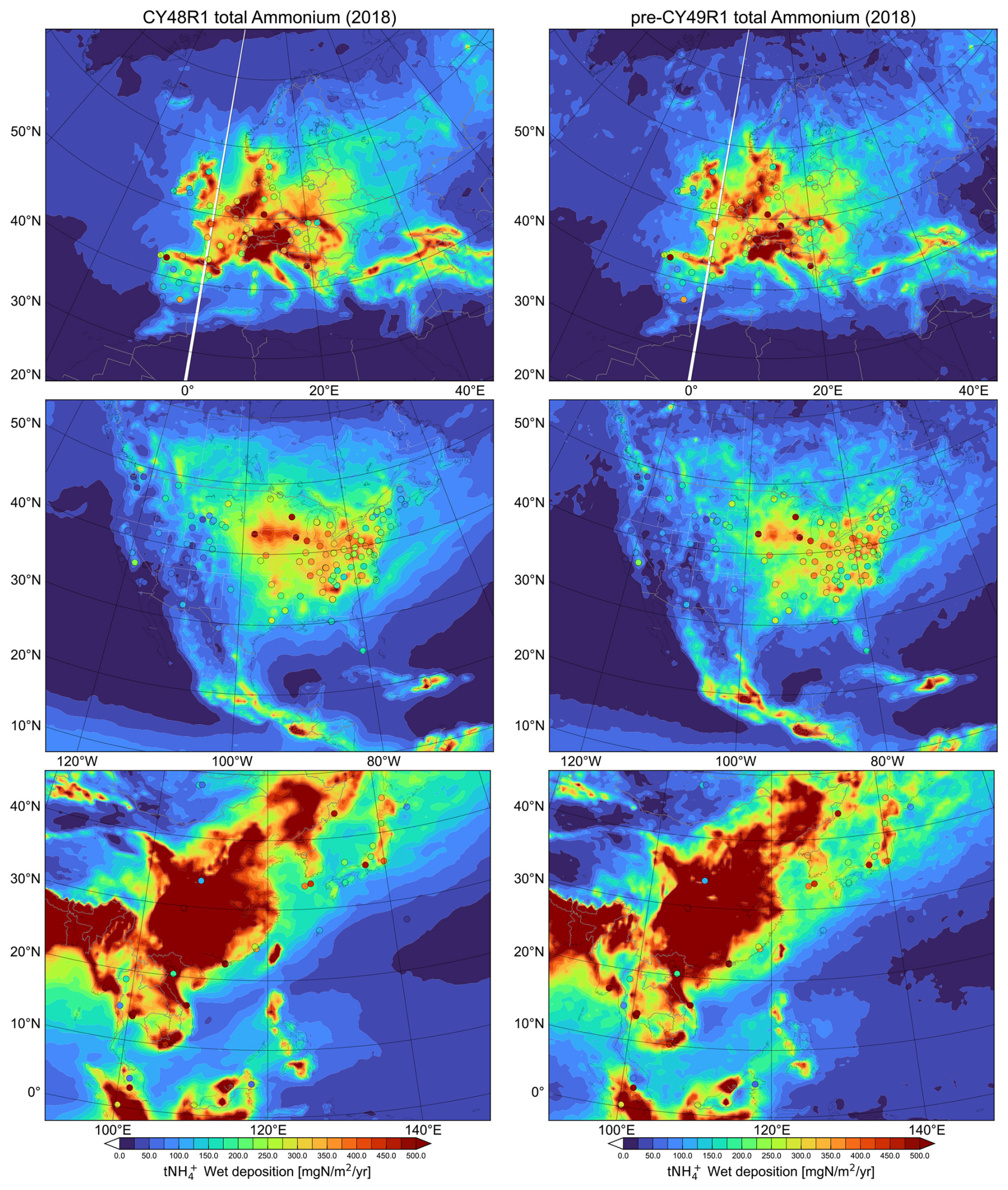
Figure 11 Yearly comparisons of the cumulative wet deposition totals of dissolved NH₃ and NH${}_{\mathrm{4}}^{+}$ aerosol (mgN m⁻² yr⁻¹) for 2018 as simulated in Cy48r1 (left column) and pre-Cy49r1 (right column) shown for Europe (top), the US (middle) and Southeast Asia (bottom). The corresponding statistics are provided in Table 9. Site locations and observed values, taken from the EMEP, CASTNET and EANET networks respectively, are shown in circles.

5.3 Total yearly wet NO_x deposition

Finally, in Fig. 12 the corresponding changes in the total yearly mean wet deposition of oxidised N for both Cy48r1 and pre-Cy49r1 during 2018 are shown. The global chemical budget terms provided in Table 6 reveal that there is an increase in the gas-phase production term for HNO₃, with a relatively constant heterogeneous conversion term for N₂O₅ when summed over the various reactive surfaces. Once formed, a significant fraction of HNO₃ is directly scavenged into aqueous cloud droplets and deposited to the surface as wet (acidic) deposition (cf. Rémy et al., 2024). However, the large biases shown for HNO₃(g) do reveal a limit to the loss via wet scavenging and deposition, with an excess remaining in the gas phase, which impacts the results shown in this section. Note that the particulate NO${}_{\mathrm{3}}^{-}$ takes various chemical forms in IFS-COMPO (Ca(NO₃)₂, NaNO₃, KNO₃, NH₄NO₃), therefore there is only partial commonality between the changes shown for NH${}_{\mathrm{4}}^{+}$ and NO${}_{\mathrm{3}}^{-}$. With the application of EQSAM4Clim in pre-Cy49r1, the surface concentration and burden of NH${}_{\mathrm{4}}^{+}$ decreases strongly, while the gas phase concentration of HNO₃ increases (cf. Tables 4 and 6; Figs. 5 and 8).

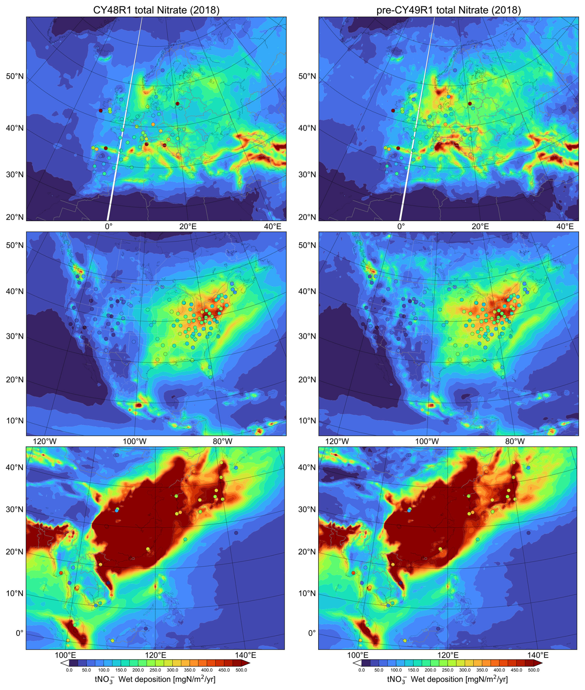
Figure 12 Yearly comparisons of the cumulative wet deposition totals of dissolved HNO₃ and NO${}_{\mathrm{3}}^{-}$ aerosol (mgN m⁻² yr⁻¹) for 2018 as simulated in Cy48r1 (left column) and pre-Cy49r1 (right column) shown for Europe (top), the US (middle) and Southeast Asia (bottom). The corresponding statistics are provided in Table 9. Site locations and observed values, taken from the EMEP, CASTNET and EANET networks respectively, are shown in circles.

For Europe (top panels), the observational yearly total wet deposition values from EMEP show that there is a rather constrained range in the deposition of total oxidised N deposition (150–275 mgN m⁻² yr⁻¹) apart from a few outliers such as on the southern coast of Ireland which have values > 500 mgN m⁻² yr⁻¹. In general, there are increases in the yearly wet deposition of [NO${}_{\mathrm{3}}^{-}$] between Cy48r1 and pre-Cy49r1, which increases the regional background totals improving agreement in e.g. Germany, which significantly reduces the yearly MB (cf. Table 9). In contrast to oxidized S, pre-Cy49r1_NOE4C simulates a reduction in the yearly wet deposition totals, for oxidized N which is further decreased for the coarse mode by applying EQSAM4Clim. The increase in [HNO₃(g)] means a larger fraction of oxidized N remains in the gas-phase thus reducing [NO${}_{\mathrm{3}}^{-}$] and improving the MB against observations as shown in Sect. 4. This subsequently leads to an improvement in performance for the regional yearly wet deposition totals. However, the large significant MB introduced for [HNO₃(g)] shows that another loss term is necessary for fully describe the budget of oxidized N across phases. For the US (middle panels), higher values of oxidised N deposition occur towards the east coast as defined by the distribution of NO_x emissions (Fig. 12). The range in the observational total wet deposition values from CASTNET is between 50–500 mgN m⁻² yr⁻¹, exhibiting a strong longitudinal gradient. Although this gradient is captured rather well, there is typically an overestimation of between 100–200 mgN m⁻² yr⁻¹ for e.g. New York state and the surrounding regions in Cy48r1. For the Western US, observations provide the range of between 0–100 mgN m⁻² yr⁻¹, with positive model biases of 100 mgN m⁻² yr⁻¹ for the northwestern states in both model versions. For the southern US, Cy48r1 exhibits overestimates of 50–70 mgN m⁻² yr⁻¹, which decreases noticeably in pre-Cy49r1. There is a large positive MB in Cy48r1 of 130 mgN m⁻² yr⁻¹ which is improved in pre-Cy49r1 decreasing by 23 %. Again, the Pearsons R value remains relatively unaffected showing the governing influence of the spatial distribution of the main point sources.

For Southeast Asia (bottom panels), the range in the EANET observational total wet deposition values is between 50–800 mgN m⁻² yr⁻¹ (not shown), with the highest values of > 2000 mgN m⁻² yr⁻¹ occurring on the Malaysian Coast. For northern and central China, total wet deposition values of up to 500 mgN m⁻² yr⁻¹ occur, covering a wide area including the similar to oxidised S. For Cy48r1, simulated values exceed observed values by 100 %–400 %, with a lack of spatial variability across the domain. Much better agreement occurs for Myanmar, Cambodia and Thailand related to much lower NO_x emissions. Comparing Cy48r1 and pre-Cy49r1 shows that a marked decrease in the MB of 31 % occurs between cycles, although the MB is at least twice that simulated for the other continents.

6 Conclusions

In this paper we build on the previous evaluations of the performance of IFS-COMPO pre-Cy49r1 presented in Rémy et al. (2024), and quantify the impact of applying the EQSAM4Clim module in IFS-COMPO for the revised calculation of aerosol and cloud pH (Metzger et al., 2024) on its ability to improve air quality forecasts of SIA. To scrutinise its effect on atmospheric composition, we have compared an operational IFS version (Cy48r1) with the next operational IFS version, which uses EQSAM4Clim in combination with a unified wet scavenging approach and other developments (pre-Cy49r1). Further improvements are also made with respect to both in-cloud and below cloud scavenging of soluble trace gases and aerosols through an implementation of updated parameterizations as detailed in Rémy et al. (2024).

EQSAM4Clim significantly influences wet deposition processes through its impact on aerosol loading and gas-aerosol partitioning. By altering the aerosol and cloud pH, the scheme modulates the chemical oxidation rates of precursor gases such as NH₃, SO₂ and HNO₃. This, in turn, affects the formation and partitioning of SIA, their hygroscopic growth, and their subsequent removal of both dry and wet deposition pathways – including in-cloud and below-cloud scavenging. These changes also influence the aerosol radiative effects, both directly and indirectly, underscoring the interconnected role of thermodynamic aerosol modeling in atmospheric composition and deposition simulations.

When applying EQSAM4Clim in a large-scale high resolution global modelling framework, we have shown that the most significant impacts of our IFS-COMPO updates concern the production efficacy of SIA and subsequent phase partitioning of reduced/oxidised nitrogen species. Comparing simulations with and without EQSAM4Clim, shows that changes in SIA are principally caused by altering the gas/aerosol partitioning as predicted. The gaseous precursors, SIA surface concentrations and wet deposition totals for the three dominant global source regions (Europe, the US, and Southeast Asia) have been evaluated against weekly/yearly observational composites for 2018.

For SO₂(g) $/$ SO${}_{\mathrm{4}}^{\mathrm{2}-}$, the conversion rate only exhibits moderate changes, with statistics being strongly impacted by the emission inventory employed. For SO₂(g), an increase in the global tropospheric burden of 7 % shows less phase transfer due to limitations in the uptake imposed by the increase in the pH of the solution. An increase in the gas phase production term of H₂SO₄(g), which is subsequently scavenged, offsets a modest reduction in the aqueous phase production term of 2 %. For surface [SO₂(g)], no significant impact has occurred with respect to the mean bias against observational means in Europe and the US. Moreover, the correlation in the weekly variability improves only marginally. For [SO${}_{\mathrm{4}}^{\mathrm{2}-}$] there is an increase in both the tropospheric burden and lifetime by one third due to the wet scavenging updates made to IFS-COMPO, with an associated reduction in the yearly mean biases for Europe and the US and increases in the corresponding correlation coefficients. However, for China there is a degradation in the performance which is associated with an increase in the positive yearly mean bias and a decrease in the correlation coefficient. For the wet deposition of oxidized S, results are mixed. Reductions in the mean bias are found for Europe and China, whilst for the US the MB increases markedly.

For NH₃(g) $/$ NH${}_{\mathrm{4}}^{+}$ the changes from applying EQSAM4Clim online are substantial, resulting in beneficial improvements in the global modelling of reduced nitrogen. For NH₃(g) the tropospheric burden almost doubles due to a halving of the conversion rate of NH₃(g) into NH${}_{\mathrm{4}}^{+}$, where more NH₃(g) is directly deposited to the surface. For surface [NH₃(g)], there is some similarity in the increases in the weekly mean bias between Europe and the US. For [NH${}_{\mathrm{4}}^{+}$], the application of EQSAM4Clim significantly reduces the associated mean bias against observational yearly means by approximately 45 % for all three global regions. This is explained by a reduction in the efficacy of particle formation, especially during summertime. For the yearly wet deposition component, the positive mean bias almost halves for Europe and the US, whilst increasing significantly for Southeast Asia. For HNO₃(g) $/$ NO${}_{\mathrm{3}}^{-}$ the changes due to EQSAM4Clim are similar to those simulated for the NH₃(g) $/$ NH${}_{\mathrm{4}}^{+}$ partitioning due to the speciation of the SIA being mainly linked via NH₄NO₃. The gas-phase production of HNO₃(g) increases by 15 %–20 % with a limited increase in the global tropospheric burden of 3 % due to compensating increases in the loss to surface via both dry and wet deposition. The application of EQSAM4Clim increases the fine aerosol component whilst reducing the coarse aerosol component, which reduces the fraction of HNO₃(g) held in the particulate phase by 50 % and increases transport lifetimes for smaller particles. For HNO₃(g) in Europe, there is a persistent negative bias during the summertime which is changed to a significant positive mean bias due to a larger fraction remaining in the gas phase. For the US, there is a degradation with a relatively low mean bias changing to a large positive bias for the entire year which indicates an incomplete process coupling when considering mineral cations without aerosol dynamics. For [NO${}_{\mathrm{3}}^{-}$], significant improvements in the yearly mean biases occur across the globe as illustrated by the three chosen regions, which comes with improvements in the simulated correlation coefficients. For the yearly wet deposition totals, there are reductions in the mean bias for all regions, without any significant change in the correlation.

In summary, although the impact on SO₂(g) $/$ SO${}_{\mathrm{4}}^{\mathrm{2}-}$ are rather small across various global regions, the impact on both particle concentrations and wet deposition totals for both reduced and oxidised N improve markedly for both Europe and the US, whereas for Southeast Asia changes are rather mixed. Significant improvements could be made by applying more accurate emission inventories and including additional anions such as chlorine from sea-salt to influence coastal regions and the significant changes simulated over the oceans in this study. Overall, the recent improvements brought by EQSAM4Clim (Metzger et al., 2024) as applied here and in Rémy et al. (2024), shows that the changes shown for pre-Cy49r1 are fit-for-purpose with respect to capturing regional particle concentration and the loss terms via wet deposition and improve the forecasting on PM at global scale.

Appendix A

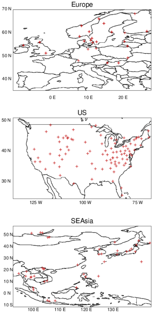
Figure A1 The location of the observational sites used for evaluating the surface concentration of SO₂ for Europe (top panel), the US (middle panel) and SEAsia (lower panel).