r.avaflow v4, a multi-purpose landslide simulation framework

We present r.avaflow  v4, an enhanced version of the open-source mass flow simulation tool r.avaflow. The updated version includes, among other new functionalities, (i) a layered model, where the individual phases move on top of each other instead of mixing; (ii) a mechanically controlled landslide deformation model, supporting the entire range from block sliding to full deformation; (iii) a slow-flow model, allowing for the simulation of landslides beyond extremely rapid processes, using an equilibrium-of-motion model; and (iv) an interface for 3D and virtual reality visualization of the results. We use four case studies to demonstrate the functionalities introduced to r.avaflow  v4 and to discuss the related chances and challenges: (i) a generic planar rock slide with interlayer shearing, and (ii)–(iv) semi-generic representations of the prehistoric Köfels rock slide (Austria), the prehistoric East Fogo landslide and tsunami (Cape Verde), and the Dösen rock glacier (Austria). Our results clearly reveal the high potential of the additional functionalities to widen the scope of r.avaflow beyond the simulation of extremely rapid and freely deforming mass flows. Combinations of the layered model, mechanically controlled deformation, and the slow-flow model unlock potentials yet barely explored in the field of GIS-based landslide simulations. In addition, the layered model facilitates a more realistic simulation of landslide-reservoir interactions. We also highlight the limitations regarding the physical basis and the application of the functionalities presented. Our enhancements are particularly useful for improved process visualization targeting at awareness building and environmental education. They are also suitable to be used for scenario-based predictive simulations in combination with a thorough empirical evaluation campaign.

1 Introduction

Mass flow simulation tools are used for numerically reconstructing, predicting, and communicating flow-type landslide processes. The first conceptual model for mass flows dates from the 1930s (Heim, 1932), and the first physically-based approach from the 1950s (Voellmy, 1955). More sophisticated models have evolved from the earlier models over time. By the mid-2020s, many practitioners still prefer physically rather simple models put into user-friendly interfaces, such as the RAMMS software (Christen et al., 2010). At the same time, scientific attention is paid to two-and multi-phase models such as OpenLISEM, integrating slope hydraulics, landslide release, and landslide runout (Bout et al., 2021) or r.avaflow, a flexible multi-phase computational framework focused on complex, cascading landslide processes, and on a full 3D implementation of the material point method (Cicoira et al., 2022).

We focus on r.avaflow, a Geographic Information System (GIS) based open-source simulation framework for mass flows and related process chains. It was first introduced by Mergili et al. (2017), at that time based on the two-phase mass flow model of Pudasaini (2012), with a solid and a fluid phase. The tool was then continuously extended and equipped with a third, fine-solid, phase (Pudasaini and Mergili, 2019). It was applied to a number of case studies, mainly regarding geomorphic process chains in high-mountain environments, such as the 2012 Santa Cruz glacial lake outburst flood (GLOF) (Mergili et al., 2018a), the complex landslides in 1962 and 1970 at Huascarán (Mergili et al., 2018b), the 2017 Piz Cengalo–Bondo process chain (Mergili et al., 2020a), the 1941 Palcacocha GLOF (Mergili et al., 2020b), the 2020 Salkantay GLOF (Vilca et al., 2021), the 2020 Jinwuco GLOF (Zheng et al., 2021), the 2021 Chamoli process chain (Shugar et al., 2021), and, most recently, the 2023 South Lhonak GLOF process chain (Sattar et al., 2025).

The various case studies have highlighted the potentials of the r.avaflow software, but also revealed remaining limitations and need for enhancement, which can be summarized as follows:

• 1.

  Forward simulations remain a particular challenge, especially for complex process chains, since parameters must be calibrated with observed and documented mass flow characteristics. Guiding parameter sets for future simulations would have to rely on a large number of back-calculations of documented events (Mergili et al., 2018b).

• 2.

  r.avaflow is only suitable for extremely rapid processes. It was not designed for slower processes dominated by viscosity. A prototype of a slow-flow model was nevertheless implemented recently (Su et al., 2024; Sect. 2.4).

• 3.

  r.avaflow is designed for more or less freely deforming flow-type processes. It is unsuitable for slide-type movements with limited deformation. However, a prototype for deformation control (Pudasaini and Mergili, 2024a) was included recently.

• 4.

  Each of the phases is clearly associated with a particular rheology, without a lot of flexibility (the solid, fine-solid and fluid phase in Pudasaini and Mergili, 2019). A Voellmy-type rheology (Voellmy, 1955) is only available with the single-phase model.

• 5.

  Even though the tool is able to cope with three phases, there is always a mixture of the phases assumed. E.g., the behaviour of a landslide moving and depositing at the bottom of a reservoir without substantial mixing with the water cannot be simulated. Preliminary computational experiments with large-scale volcanic flank collapses have revealed a strong need to revisit and to enhance the concepts of r.avaflow in regard to the simulation of landslide-to-reservoir impacts.

• 6.

  The user interface basically consists in a start script which has to be written manually, without a capable user interface. The software is tightly coupled with the Geographic Information System GRASS GIS (GRASS Development Team, 2025) and bound to UNIX systems.

• 7.

  Raster maps, text files and map and animation plots are provided as output, but there are no direct interfaces to more advanced visualization systems.

We do not consider challenge (1) in this work. The issue of guiding parameter sets and forward simulations has to be the subject of further investigations, e.g., by applying machine learning and artificial intelligence methods (Yildiz et al., 2023). Instead, we focus on the challenges (2)–(7), along with some other aspects, to enhance the scope and usability of the r.avaflow mass flow simulation framework. We note that for (2), (3), and (5), we are not aware of any comparable software tools appropriately dealing with the challenges mentioned. In Sect. 2, we will introduce r.avaflow  v4 and its new functionalities, compared to the older versions. Furthermore, in Sects. 3 and 4 we will demonstrate the functionalities using a set of generic and semi-generic case studies. We will discuss our findings in Sect. 5 and conclude in Sect. 6.

2 The simulation framework r.avaflow

2.1 General concept of r.avaflow

r.avaflow is a GIS-based open-source mass flow simulation framework. The model applies physically-based equations to numerically estimate and calculate the motion of mass and momentum of up to three phases through a regular grid. The two-phase model of Pudasaini (2012) was employed in the original version (Mergili et al., 2017). It was later upgraded by the three-phase model of Pudasaini and Mergili (2019), with a solid, a fine-solid, and a fluid phase, each associated with pre-defined rheologies: the solid phase is characterized through internal and basal friction, the fine-solid phase additionally through viscosity and yield strength, and the fluid phase through viscosity and yield strength. Interactions between the phases are considered through buoyancy effects, virtual mass, and drag. A Voellmy-type mixture model is available as an alternative. The mass and momentum balance equations in Pudasaini and Mergili (2019) are depth-averaged, and the phases are considered to be mixed over the flow height, even though the vertical distribution of the concentration of the individual phases can be controlled. A TVD-NOC (Total Variation Diminishing Non-Oscillatory Central Differencing) scheme on a staggered grid is used for mass and momentum transport (Tai et al., 2002). We use the scheme in the way described by Wang et al. (2004).

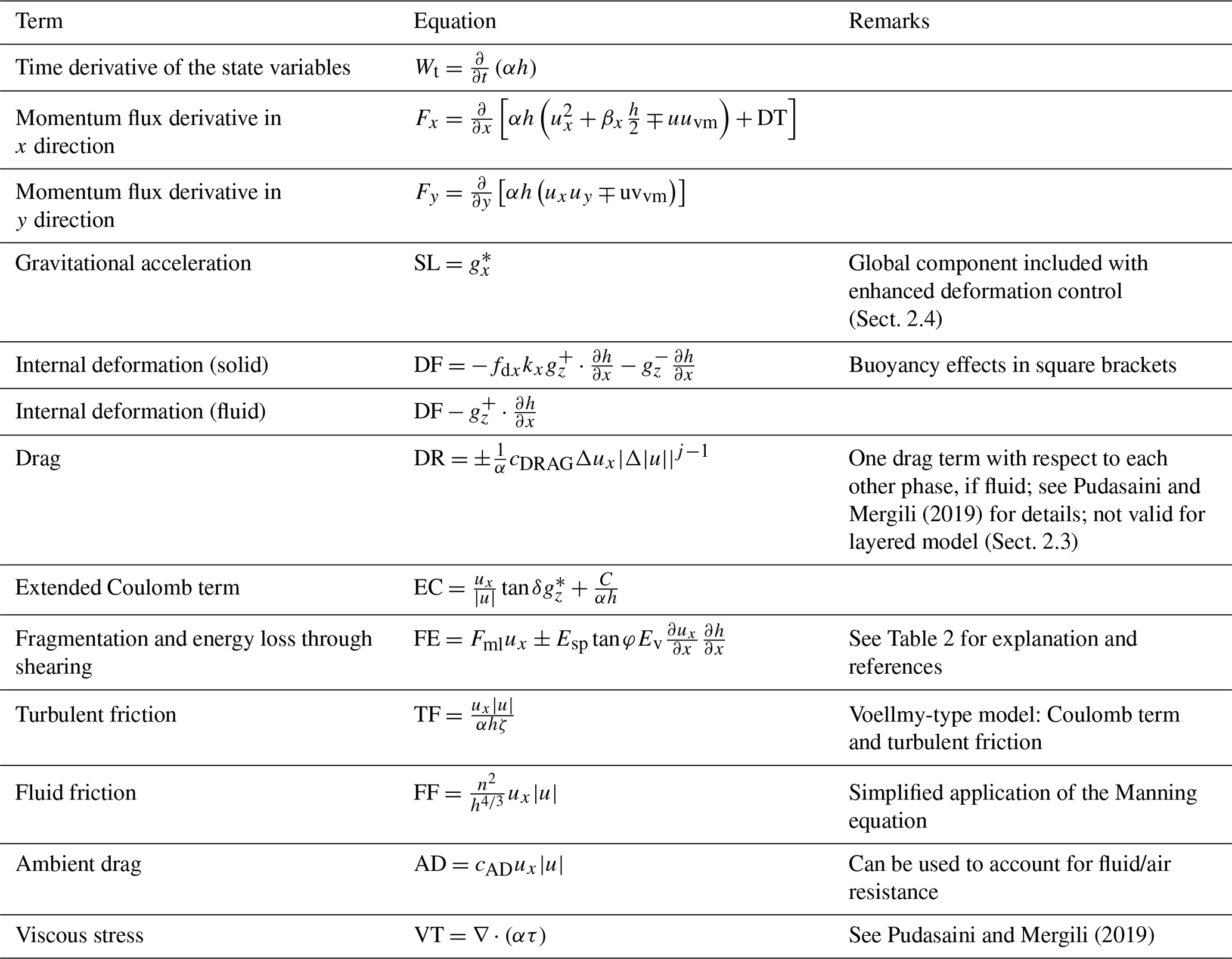
Table 1 x-directional flux and source terms governing flow dynamics in r.avaflow  v4, for any of the maximum of three phases. Terms in y direction are formulated in an analogous way. u_x and u_y = depth-averaged velocities in x and y direction; uu_vm and uv_vm = virtual mass contributions (Pudasaini and Mergili, 2019); DT = dispersion term (Pudasaini, 2023); $g_x^{\ast }$ = effective downslope component of gravity in x direction; f_dx = deformation coefficient in x direction (Pudasaini and Mergili, 2024a); k_x = x-directional earth pressure coefficient; $g_z^{+}$ and $g_z^{-}$ = effective slope-normal components of gravity, including the different buoyancy effects (Pudasaini and Mergili, 2019); $g_z^{\ast }$ = effective slope-normal components of gravity, including buoyancy and curvature effects; c_DRAG = drag coefficient (Pudasaini and Mergili, 2019), corrected for the relevant buoyancy effects; Δu_x = velocity difference in x direction with respect to another phase; Δ|u| = difference in absolute velocities with respect to another phase; δ = basal friction angle; c = cohesion; E_v = energy loss through shearing coefficient (Pudasaini and Mergili, 2024b); φ = internal friction angle; F_ml = fragmentation number (Pudasaini et al., 2024); ζ = turbulent friction number; n = Manning number, accounting for the roughness of the basal surface for the fluid phase; c_AD = ambient drag coefficient, and τ = viscous stress. Bold letters denote input parameters.

Typically, the release mass is defined through raster maps showing the release heights for each cell and each phase, imposed on a digital terrain model. Hydrographs defined by discharge and flow velocities are provided at those locations (not only for water, but for all types of materials considered in r.avaflow) and can also be used for the input of mass and momentum to the system. Additional functionalities include entrainment, stopping, non-hydrostatic dispersive motion, spatio-temporal variation of several parameters and controls, and empirical evaluation of the results. The readers are directed to the r.avaflow web site (Mergili and Pudasaini, 2025) for further information. The output of r.avaflow essentially consists in time series of ascii raster maps and plots of flow height and (optionally) kinetic energy and dynamic pressure, along with text files summarizing the simulation.

2.2 New features of r.avaflow  v4

In contrast to earlier versions of r.avaflow, with pre-defined solid, fine-solid, and fluid phases (Pudasaini, 2012; Mergili et al., 2017; Pudasaini and Mergili, 2019), there is no a-priori distinction between different rheologies in r.avaflow  v4: rheologies are automatically determined, depending on the user input. For the sole purpose of representation, we provide a quick and informal overview of the multi-phase momentum balance equation:

$$\begin{array}{}\text{(1)}& \begin{array}{rl}{W}_{\mathrm{t}}+F_x+G_y& =\mathit{\alpha }hH(\text{GA},\text{DF},\text{DR},\text{EC},\text{FE},\\ & \text{TF},\text{FF},\text{AD},\text{VT})\end{array}\end{array}$$

For the rigorous, formal descriptions of the model equations, we refer to Pudasaini and Mergili (2019) and the other relevant references mentioned above and in Table 1. Equation (1) applies to the x and y directions for each of the (minimum 1, maximum 3) phases. The flux terms W_t, F_x, and G_y are expressed as the time derivatives of the state variables, and the momentum flux derivatives in x and y direction. α is the volumetric fraction of the relevant phase, and h is the total flow height. H is a function of all the applied forces: the gravitational acceleration (GA), internal deformation (DF), drag (DR), an extended Coulomb term (EC), fragmentation and energy loss through shearing (FE), turbulent friction term (TF), fluid friction term (FF), ambient drag term (AD), and the viscous stress terms (VT). We note that EC, FE, TF, FF, AD, and VT can only decelerate motion. This implies that, in sum, these terms do not induce a change in the direction of motion. From a purely mathematical point of view, the flow at the given raster cell would stop if such a change of direction would occur. All terms are elaborated in more detail in Table 1. All key parameters used in the equations of Table 1 can be defined as global values or as raster maps, where individual values can be provided for each raster cell. Detailed information on all aspects exceeds the scope of this work and is provided in the referenced publications in Table 1.

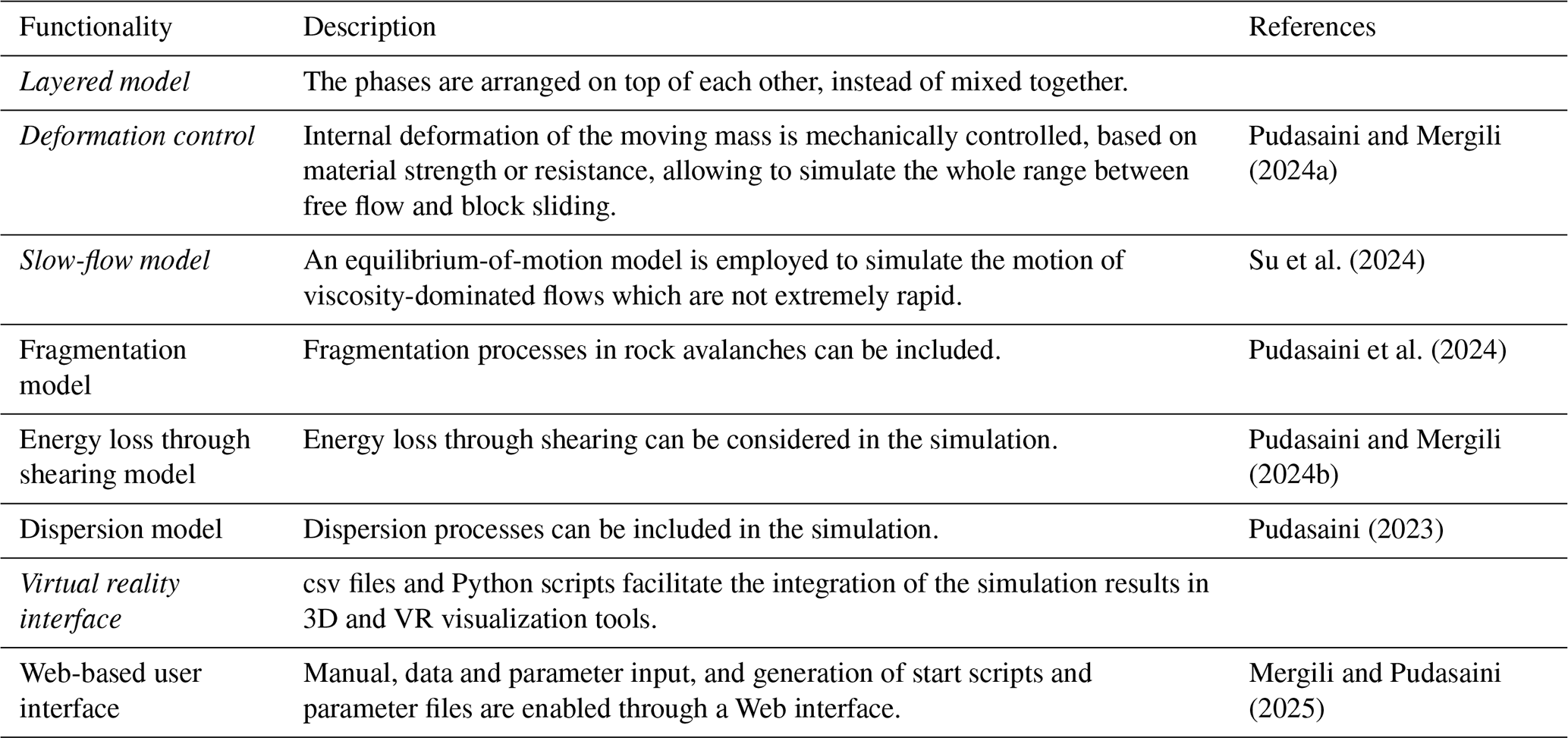
Table 2 Additional functionalities available in r.avaflow  v4. Those functionalities considered in detail in this study are written in bold letters.

The behaviour of the landslide depends on the definition of the parameters associated to each term. All terms can be deactivated by setting the governing input parameters to zero. Where necessary, it is automatically decided whether to consider a material as solid or as fluid: solid material is assumed if the internal friction angle φ > 0. Otherwise, the material is considered fluid. Buoyancy is only considered with respect to fluid phases of lower density. Not all combinations of terms are necessarily physically meaningful, so that the enhanced flexibility for users also implies an increased responsibility to combine terms in a meaningful way.

The Voellmy-type model is available for each phase, by combining the Coulomb term with the turbulent friction term. Apart from rethinking the general concept of the phases, some additional functionalities have been introduced (some of them as prototypes already in the previous version r.avaflow v3). They are summarized in Table 2.

The models for fragmentation (Pudasaini et al., 2024), energy loss through shearing (Pudasaini and Mergili, 2024b), and dispersion (Pudasaini, 2023), which have been introduced earlier, will not be further discussed here. The model for deformation control has been presented by Pudasaini and Mergili (2024a), but an enhanced version is used in the case studies presented in Sect. 3. We now introduce the layered model, the enhanced deformation control, the slow-flow model, and the virtual reality interface. We point out that all these models can be combined with each other (Sects. 3 and 4).

2.3 Layered model

When a landside hits a reservoir, simulation with a depth-averaged multi-phase mixture model results in a mixture of solid landslide material and fluid water. The solid and fluid column of material is not resolved, and the phases are mixed along the vertical or slope-normal profile of the flow mass. For example, for a two-phase model involving a frictional solid phase, this means that the entire column of material is effectively frictional. The way the pressure gradients are computed will prevent the fluid phase from behaving independently from the solid phase. In situations where the solid fraction is significant, the original water surface might not recover, depending on the specific situation and model parameterization. Such a behaviour is not realistic in those cases where a landslide deposits at the bottom of a reservoir. This phenomenon is particularly obvious in the results of simulations where large landslides deposit at the bottom of deep reservoirs, whereas it is less clearly visible where small landslides interact with rather shallow water bodies.

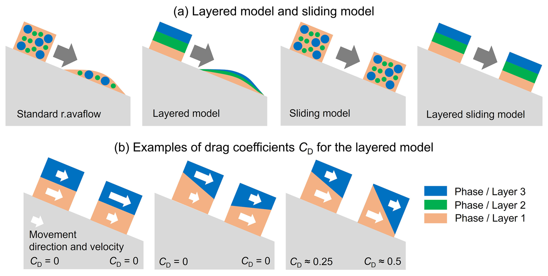
Figure 1 Schematic sketch illustrating the effects of the new model components of r.avaflow  v4, using profiles along the down-slope direction. (a) Comparison of the standard model used in r.avaflow, with maximum 3 phases (Pudasaini and Mergili, 2019); the layered model, where the phases are not mixed, but arranged on top of another; the model with deformation control, where the deformation of the moving mass is controlled; and the combination of the layered model and the deformation control. (b) Examples of drag coefficients computed with the layered model (examples here with two distinct layers) for selected idealized situations.

In many real-world-cases, however, we can assume such a solid-dominated bottom and a fluid-dominated top, connected by a mixture layer. In the present work, we simplify this pattern to a maximum of three layers, with phase 1 at the bottom, an optional phase 2 in the middle, and phase 3 at the top, i.e., the individual phases are arranged on top of each other instead of mixed together (Fig. 1a). Thereby, each layer represents one phase, meaning that individual layers cannot be multi-phase. To achieve this, we control the gravity components, the flow height gradients, and the drag forces:

Gravity components $g_x^{\ast }$, $g_y^{\ast }$, $g_z^{\ast }$, $g_z^{+}$, and $g_z^{-}$: with the layered model, the gravity components for phase 2 and phase 3 are not computed from the slope of the basal surface, but from the slope of the upper surface of the layer below. This means that the upper surface of phase 1 is considered the basal surface of phase 2, and the upper surface of phase 2 is considered the basal surface of phase 3. Buoyancy effects on the gravity components are not considered for the layered model.

Flow height gradients ∂h/∂x and ∂h/∂y: in the standard mixture model introduced in Sect. 2.1, the effective flow height for internal deformation is the total mixture height h_e = h. In the layered model each phase P1–P3 has its own effective material height, h_e = h_P1 for phase 1, h_e = h_P2 for phase 2, and h_e = h_P3 for phase 3. This ensures that each phase deforms individually, but with the effect of the evolving geometry of the underlying phase.

Drag DR: with the standard model, the drag is computed according to Pudasaini and Mergili (2019) for each phase in the mixture. This concept, however, is not applicable to layered movements, for which we introduce the following approximation for the drag coefficient in x direction C_Dx:

$$\begin{array}{}\text{(2)}& \begin{array}{rl}\text{if }\text{sgn}{\displaystyle \frac{\partial h_{\mathrm{P}\mathrm{1}}}{\partial x}}=& \text{sgn}\left(u_{x,P\mathrm{2}}-u_{x,P\mathrm{1}}\right)\\ & \text{ and }\mathrm{|}{u}_{x,P\mathrm{1}}\mathrm{|}>\mathrm{|}{u}_{x,P\mathrm{2}}\mathrm{|}:C_{\mathrm{D}x}\\ =& f_{\text{DR}}\cdot \sin \left(\text{arctan}{\displaystyle \frac{\partial h_{\mathrm{P}\mathrm{1}}}{\partial x}}\right)\cdot {\mathit{\alpha }}_{\mathrm{P}\mathrm{1}},\end{array}\end{array}$$

where P2 is a fluid phase moving on top of a solid phase P1. f_DR is a scaling factor. The drag coefficient in y direction C_Dy is computed in an analogous way. If the condition given in Eq. (2) is not met, C_Dx is set to 0. Note that P1 and P2 are only used as an example. The same principle applies to combinations of P1 and P3 or P2 and P3. The ideas behind this concept are that (i) drag only acts if the thickness gradient of the solid phase goes into the same direction as the relative velocity difference between the fluid and the solid phase; (ii) drag only acts when the solid moves faster than the fluid: and (iii) the drag coefficient is proportional to the sine of the gradient of solid flow height (i.e., there would be no drag if the surface of the solid part of the flow would run parallel to the terrain slope and, theoretically, the drag coefficient would be 1 in the case of a vertical wall and f_DR = 1). Figure 1b illustrates some selected examples of drag coefficients (assuming f_DR = 1) computed with this approach.

We note that the layered model is not only useful for landslide-reservoir interactions, but also for layered landslides (Sects. 3 and 4).

2.4 Enhanced deformation control

We use the controlled deformation model introduced by Pudasaini and Mergili (2024a). This model can be applied to all phases with internal friction angle φ > 0 and builds on the effective deformation factors f_dx in x direction and f_dy in y direction, both in the range 0–1, where f_dx, f_dy = 0 completely locks the deformation (as shown in Fig. 1a), and f_dx, f_dy = 1 allows full deformation (identical to the model without deformation control). f_dx and f_dy are no input parameters. The input value is the raw deformation factor $f_{\mathrm{d}}^{\ast }$, which is enhanced with the earth pressure coefficient K and the gravity components in z direction g_zx or g_zy, respectively:

$$\begin{array}{}\text{(3)}& f_{\mathrm{d}x}=\mathrm{1}-{\displaystyle \frac{\left(\mathrm{1}-f_{\mathrm{d}}^{\ast }\right)g_z^{\ast }}{K{g}_{zx}}},f_{\mathrm{d}y}=\mathrm{1}-{\displaystyle \frac{\left(\mathrm{1}-f_{\mathrm{d}}^{\ast }\right)g_z^{\ast }}{K{g}_{zy}}},\end{array}$$

where $g_z^{\ast }$ is the gravity component in z direction at the steepest raster cell of the release area.

In cases where landslides move as one rigid block, it might be reasonable to assume that the motion of the entire block is governed by global values of the gravity components, applied to each raster cell instead of the local gravity components depending on the local slope components. For this purpose, the global gravity components $g_x^{\mathrm{g}}$, $g_y^{\mathrm{g}}$, and $g_z^{\mathrm{g}}$ are introduced, representing the mean values of the local gravity components g_x, g_y, and g_z over the entire sliding mass, weighted for flow height and updated at each time step of the simulation. Global gravity components are optionally applied in the gravitational acceleration term (g_x = $g_x^{\mathrm{g}}$, g_y = $g_y^{\mathrm{g}}$) and the deceleration term (g_z = $g_z^{\mathrm{g}}$) for frictional material. For simplicity this is referred to as global sliding, whereas the conventional way to consider each raster cell individually is referred to as local sliding. Global and local sliding can also be combined, with the parameter f_g denoting the fraction of global sliding.

2.5 Slow-flow model

Hungr et al. (2014) describe all landslides moving at > 5 m s⁻¹ as extremely rapid. This velocity class roughly defines the scope of the momentum balance model used in r.avaflow. To extend the applicability to slower landslides, an equilibrium-of-motion model has been adopted. This method, outlined by Su et al. (2024), is founded on the premise of a viscous downslope mass flow, with the flexibility to include a viscous base layer of minor thickness. It represents a simple and intuitive approach, at the cost of neglecting or simplifying some aspects, such as the evolution of pore water pressure.

Assuming a planar Couette flow, the viscous forces in x and y direction are counterbalancing the gravitational force, which substitutes the forces exerted by the upper surface. Regarding the properties of individual cells, the mass is proportional to the landslide height h, while the landslide density ρ and the surface area A are normalized:

$$\begin{array}{}\text{(4)}& \begin{array}{rl}{F}_{\mathrm{L}}=\mathit{\mu }A{\displaystyle \frac{u}{h}}& \to ahA\mathit{\rho }=\mathit{\nu }\mathit{\rho }A{\displaystyle \frac{u}{h}}\\ & \to g_{x}h=\mathit{\nu }{\displaystyle \frac{u_{x\mathrm{e}}}{h}},g_{y}h=\mathit{\nu }{\displaystyle \frac{u_{y\mathrm{e}}}{h}}\\ & \to u_{x\mathrm{e}}={\displaystyle \frac{g_x{h}^{\mathrm{2}}}{\mathit{\nu }}},u_{y\mathrm{e}}={\displaystyle \frac{g_y{h}^{\mathrm{2}}}{\mathit{\nu }}},\end{array}\end{array}$$

where F_L is the force acting on the landslide mass, μ and v are the dynamic and kinematic viscosities, u is the flow velocity at the upper surface of the landslide, a is the acceleration of the landslide, and g_x and g_y are the downslope gravity components in x and y direction. u_xe and u_ye are the equilibrium velocities in x and y directions.

Multiplying u and v by h, yields the normalized momenta p_x and p_y. Thus, the velocities of the deforming mass (u_x in x direction and u_y in y direction) decrease linearly along the vertical profile from top to bottom (base velocities u_xb, u_yb). Accordingly, u_x and u_y represent the mean velocities within the landslide column of the depth-averaged model, while the surface velocities of the landslide are $\left[\mathrm{2}\right(u_x-u_{x\mathrm{b}}\left)\right]+u_{x\mathrm{b}}$ and $\left[\mathrm{2}\right(u_y-u_{y\mathrm{b}}\left)\right]+u_{y\mathrm{b}}$. The first terms of Eq. (5) thus describe the deformation of the landslide and the second terms represent the basal movement.

$$\begin{array}{}\text{(5)}& p_x=h\left({\displaystyle \frac{g_{x\mathrm{t}}{h}^{\mathrm{2}}}{\mathrm{2}\mathit{\nu }}}+{\displaystyle \frac{g_{x\mathrm{b}}^{\ast }}{\mathit{\xi }}}\right),p_y=h\left({\displaystyle \frac{g_{y\mathrm{t}}{h}^{\mathrm{2}}}{\mathrm{2}\mathit{\nu }}}+{\displaystyle \frac{g_{y\mathrm{b}}^{\ast }}{\mathit{\xi }}}\right),\end{array}$$

where g_xt and g_yt are the downslope components of gravity in x and y direction at the top of the landslide (i.e., including gradients of flow height), v is the kinematic viscosity of the mass, and $g_{x\mathrm{b}}^{\ast }$ and $g_{y\mathrm{b}}^{\ast }$ are the downslope components of the effective gravity (Sect. 2.3) in x and y direction at the bottom of the landslide. The ratio between the kinematic viscosity of the basal layer and the square of the basal layer thickness is represented by ξ.

Mass and momentum fluxes between cells follow the conventions of traditional flow models (Savage and Hutter, 1989; fluid terms in Pudasaini, 2012; Pudasaini and Mergili, 2019). Calculating momenta from Eq. (5) results in their evolution in equilibrium with accelerating and decelerating forces at the individual grid cells. Hence, those momenta cannot act as source of momentum production or dissipation. Compared to momentum balance models one major advantage is the simple approach to time-scaling. Time-scaling can be directly applied to u and v, without the necessity to adjust any additional variables. It is important to emphasize that the outlined method neglects inertial effects and consequently must not be applied for the simulation of extremely rapid mass flows (according to the definition of Hungr et al., 2014).

2.6 Virtual reality interface

r.avaflow  v4 includes an interface for 3D and virtual reality (VR) visualization of the model results. For this purpose, a time series of csv files – one for each output time step, based on a fixed interval defined by the user – is automatically produced, describing the geometric information (elevation of the landslide surface and, optionally, elevation of the terrain surface and individual layers) for each raster cell along with red, green, and blue (RGB) colour values to be used for visualization. The RGB values are composed of the following pieces of information, which can be combined in different ways:

• landslide heights and composition of phases (updated for each time step);

• shaded relief information (updated for each time step);

• and orthophoto information, if an orthophoto is provided by the user. Optionally, the raster cell values of the orthophoto can be shifted to follow the motion of the landslide, allowing for a more realistic visualization.

Along with the csv files, Python scripts are automatically generated to facilitate import to the 3D and VR visualization and animation tools Paraview and Blender, and to the game engine Unreal Engine 5. This workflow allows for the integration of r.avaflow  v4 simulation results with various levels of virtual reality.

3 Test cases and simulation design

3.1 Generic planar rock slide with interlayer shearing

A computer-generated simplified landscape with an extent of 5000 m × 5000 m is used for the demonstration of a planar rock slide, assuming the involvement of three discrete layers of rock. An inclined slope with a gradient of 0.5 runs out into a horizontal plane in down-slope (x) direction. The three planar sliding planes are aligned parallel to the main slope. They form the bases of the top, middle, and bottom layers, with heights of 100 m each (Fig. 2).

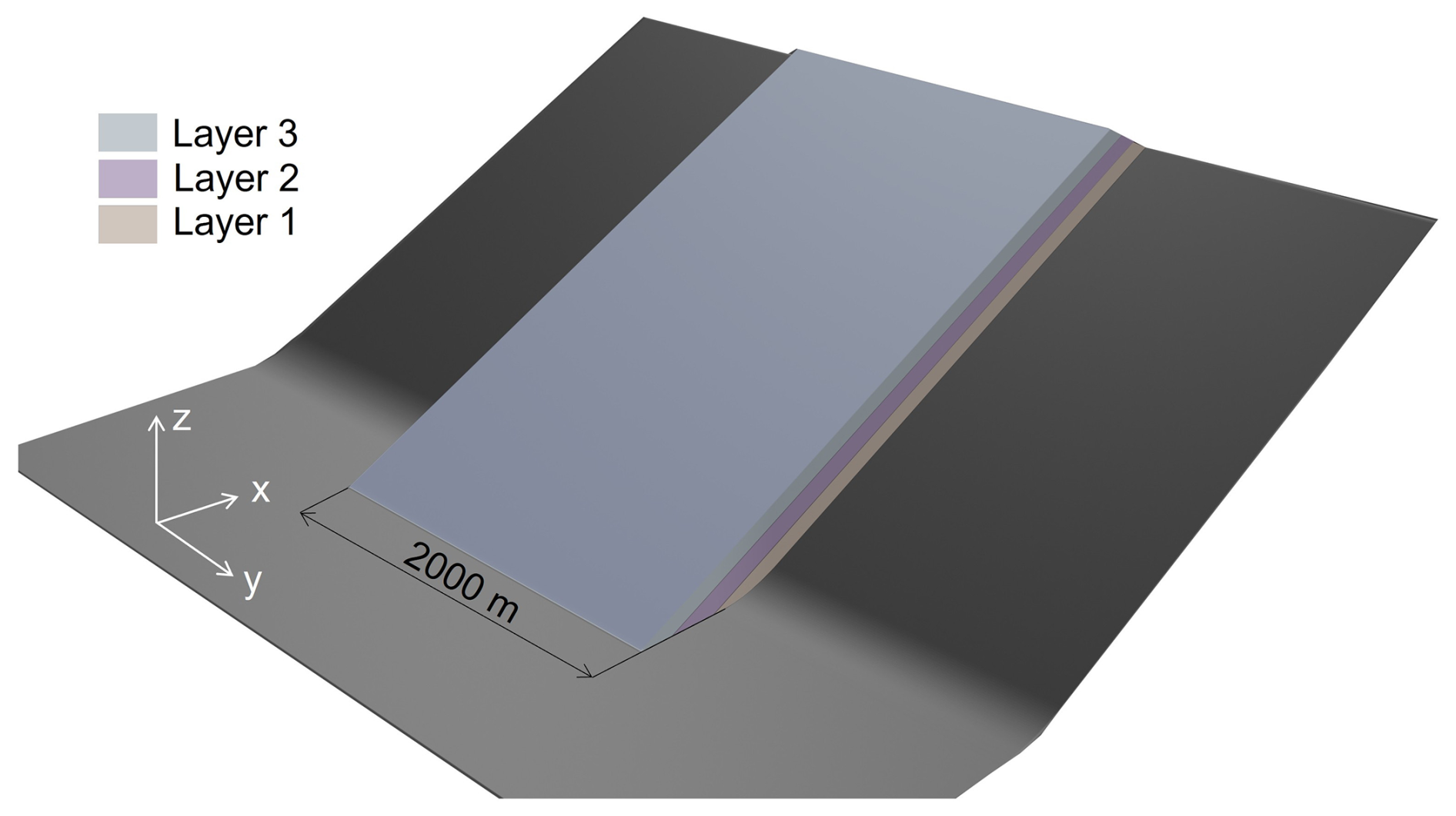
Figure 2 Oblique view of the generic landscape with a three-layer release mass, used for the experiment SD1 on a planar rock slide. The main bodies of all layers are of equal thickness (100 m), and the surfaces of the two lower layers (not visible in this view) are arranged parallel to the surface of the upper layer.

Table 3 Summary of the key parameter settings applied to the simulations on the generic slope deformation (SD1), the prehistoric Köfels rock slide (KF1–KF3), the prehistoric East Fogo event (FO1–FO3), and the semi-generic Dösen rock glacier (DO1). L = layered model.

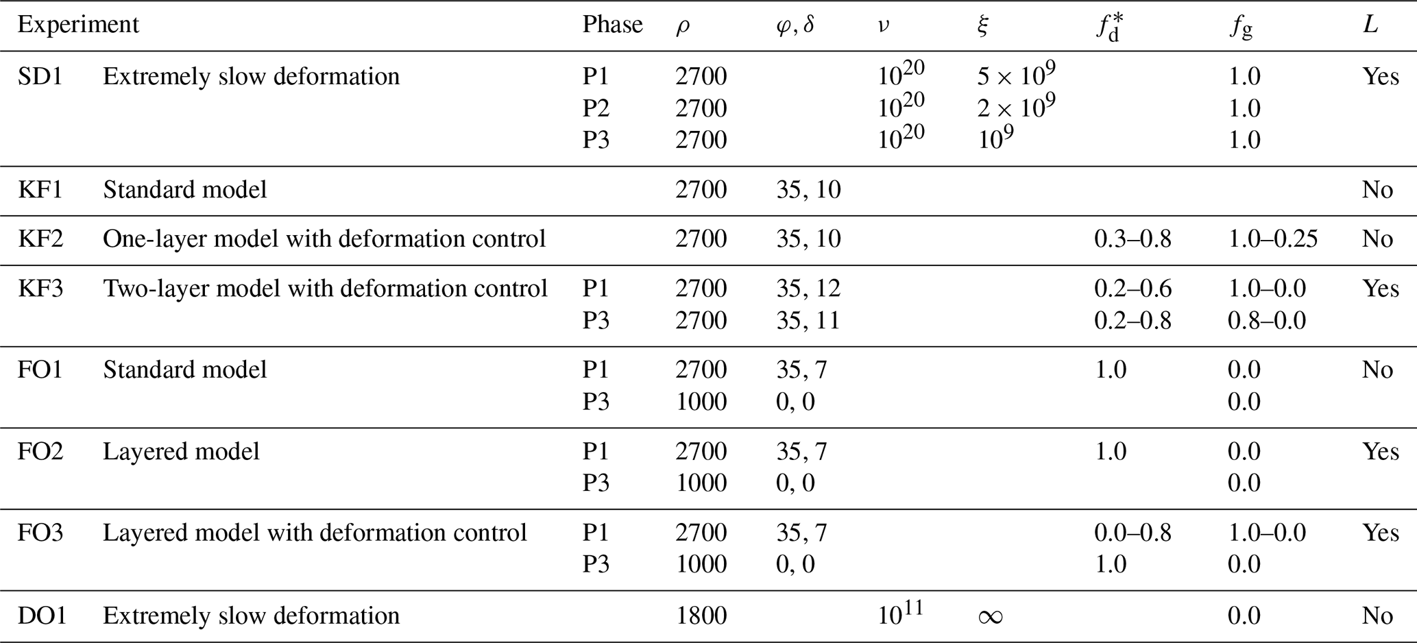
Experiment SD1 uses the equilibrium-of-motion model, assuming an extremely slow movement. Model parameters are calibrated towards a plausible representation of layered sliding, where the motion along the sliding planes clearly dominates over the internal deformation of the individual layers. The settings are detailed in Table 3. All simulations are executed with densities of ρ = 2700 kg m⁻³, and at a raster cell size of 10 m. The simulation is run for a process duration of 50 000 years, using a time scaling factor of 31.536 × 10⁹ (1 s → 1000 years).

3.2 Semi-generic Köfels rock slide

The Köfels rock slide (Fig. 3) has been thoroughly examined for more than a century (cf. Mergili and Prager, 2022 and references therein). The most recent reconstruction by Zangerl et al. (2021) builds the foundation for this case study. According to ¹⁴C-dating the event occurred 9527–9498 years before present (Nicolussi et al., 2015). The process originated from a head scarp at the western slope of the central Ötz Valley, Austria, where the steep terrain exhibits a dip angle of 40 to 80°. The centre of the mass was displaced 2.6 km downslope (Sørensen and Bauer, 2003). Erismann et al. (1977) suggested a movement velocity of 50 m s⁻¹.

The moved volume amounts to 3–4 km³ and rock mass fragmentation and fracturing induced an increase by a factor of 1.26 (Zangerl et al., 2021). The sliding rock mass reached the entrance of the tributary Horlach Valley on the opposite side of the slope, where massive bedrock forced a halt. Up to the present day, the deposit is blocking the main valley. The sliding rock mass possibly split up, as proposed by Erismann and Abele (2001): the lower part might have stopped and deposited after the collision with the opposite slope, whereas the upper part moved one kilometre farther. Preuss (1986) reported about some evidence of a potential internal shear zone. This finding, however, has not yet been supported by field evidence. An alternative more likely scenario is the emergence of several internal shear zones facilitating the adaptation to the terrain surface over the course of the substantial deformation of the rock mass. The rock slide deposit is extremely heterogeneous, with characteristics ranging from completely disintegrated and crushed material to almost solid fractured rock. The pronounced vertical and horizontal variability in the degree of cataclasis and fracturing indicates complex internal deformation phenomena during the rock slide. We consider this case study semi-generic, as there are considerable uncertainties regarding the pre-event topography and the characteristics of the rock slide and its internal deformation. Three computational experiments are performed (Table 3), using the standard flow model of r.avaflow (experiment KF1), the one-layer model with deformation control (KF2), and the multi-layer model with two layers and deformation control (KF3). For the multi-layer model, we assume a release mass composed of two layers of equal height distribution. All simulations only consider the released rock mass whereas, for simplicity, possibly entrained valley fill is neglected. The model parameters are optimized against the observed travel distance and deposit using an iterative trial-and-error procedure. Thereby, a time dependency of the deformation control and the fraction of global sliding is considered, in order to account for effects of increasing crushing and loss of coherence, related to the dynamic stresses the sliding mass is exposed to. All simulations are run with a density of ρ = 2700 kg m⁻³ and at a raster cell size of 15 m, considering a process duration of 120 s.

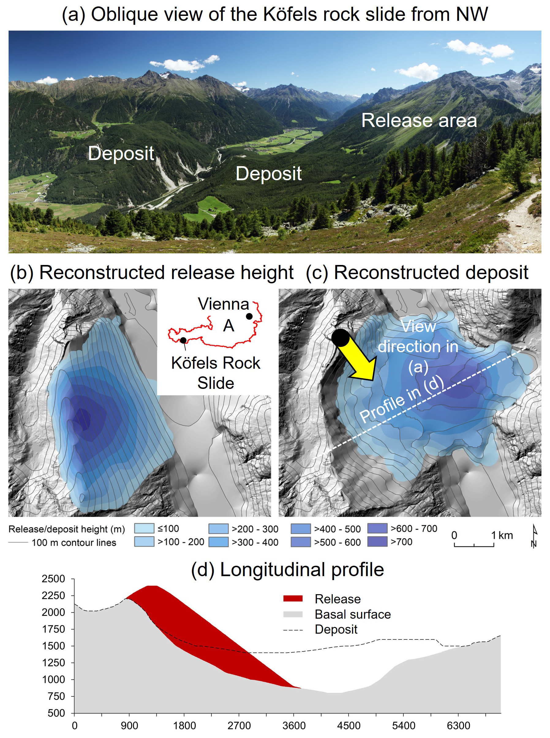
Figure 3 The prehistoric Köfels rock slide. (a) Oblique view from NW direction – author: M. Mergili (3 August 2015); (b) and (c) reconstructed release and deposition masses – modified after Zangerl et al. (2021); (d) longitudinal profile through the rock slide area from SW to NE.

3.3 Semi-generic East Fogo landslide and tsunami

Fogo is an active volcanic island, that forms part of the Cape Verde archipelago in the Atlantic Ocean off the coast of Senegal, West Africa. Its highest peak is the stratovolcano Pico do Fogo (2829 m a.s.l.), which sits at the bottom of a cauldron, bordered by a semi-circular, up to 1000 m high escarpment on the western, south-western, and north-western sides, and merging with the outer slope of the island on the eastern side (Fig. 4a). Various studies have investigated the volcanic and geomorphological history of the island, and there is broad agreement upon the fact that the cauldron was formed by giant landsliding, probably in various stages, and today's Pico do Fogo formed afterwards (e.g., Day et al., 1999; Marques et al., 2019; Barrett et al., 2020; Cornu et al., 2021). This has led to considerations of future risk. Possible tsunami deposits were found on the neighbouring island of Santiago, but their real origin is disputed, and so are the number and total volume of landslides, ranging from 20–300 km³, depending on the interpretation of the available evidence and the way of reconstructing the pre-event terrain.

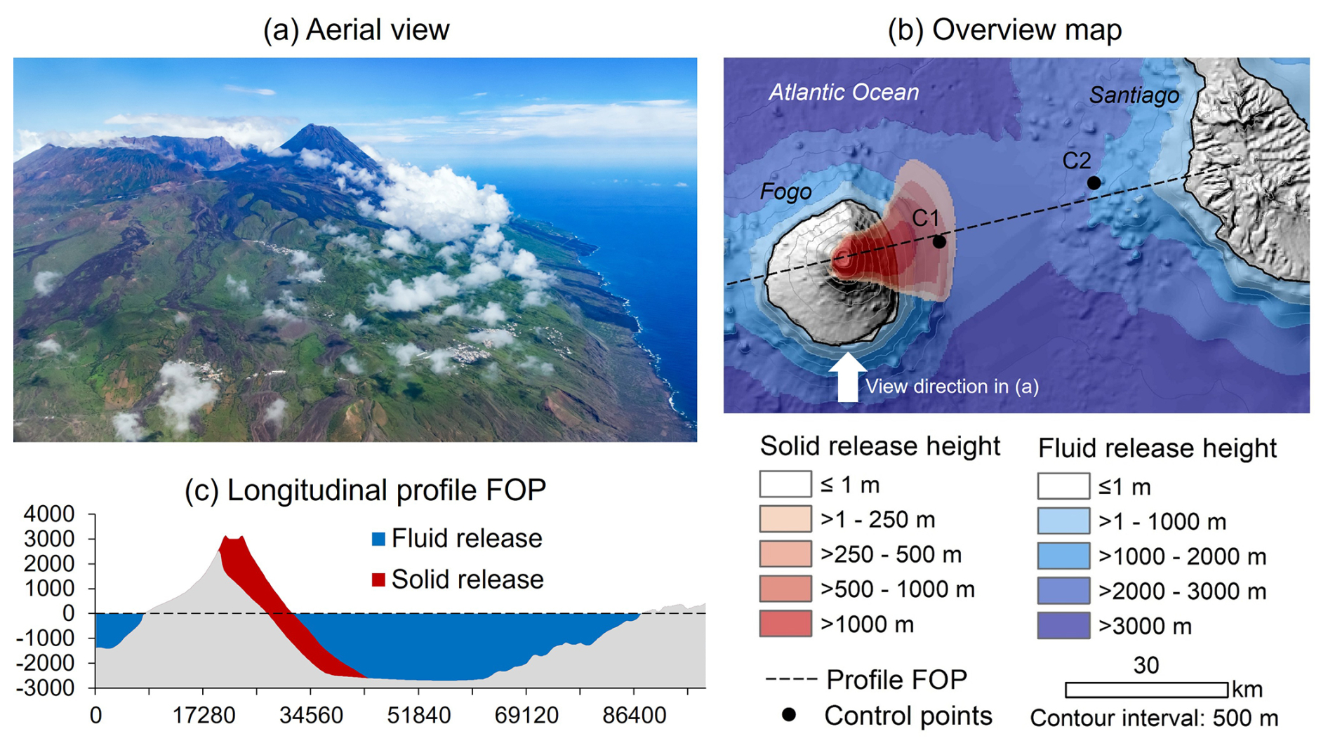
Figure 4 Prehistoric East Fogo event. (a) Aerial view of today's situation with Pico do Fogo – author: Martin Mergili (10 September 2022); (b) Overview map with reconstructed release height distribution; (c) profile along the dashed line in (b).

The aim of the present work is not to reconstruct the landsliding – often referred to as the East Fogo volcanic flank collapse(s) – in all detail, but we use this case to demonstrate the effects of layering and controlled deformation for a very large phenomenon. Our terrain reconstruction builds on the hypothesis of the existence of a former volcanic summit, named Monte Amarelo (Cornu et al., 2021), which collapsed in one single event, and the sliding surface reaching down to the basis of the volcanic edifice in the deep sea (worst-case assumption). Though our reconstruction is based on the available topographic evidence, using the SRTM V4 (Jarvis et al., 2008) and the GEBCO_2021 Grid (GEBCO Compilation Group, 2021) digital terrain models, it largely relies on the subjective reconstruction of the former terrain surface and the basal sliding surface. As a result, we characterize the outcome as a semi-generic data set (Fig. 4b and c). The derived collapse volume would be approx. 250 km³, which comes close to the maximum estimate of Day et al. (1999) (300 km³) and is much higher than more recent estimates of maximum 160 km² (Martínez-Moreno et al., 2018).

Three computational experiments are applied to the semi-generic East Fogo event (FO1–FO3). They are computed at a raster cell size of 270 m and for a duration of 900 s. The key parameters for each of the experiments are summarized in Table 3. For comparison, all simulations are repeated with the landslide material only, neglecting the ocean water.

3.4 Semi-generic Dösen rock glacier

Since the 1990s, the Dösen rock glacier has been an important site for interdisciplinary permafrost and periglacial research in the eastern Austrian Alps (Kellerer-Pirklbauer et al., 2018). Located at the valley head, this rock glacier extends over roughly 1 km in length with a maximum width of approx. 340 m, resulting in an area of some 0.2 km² (Fig. 5). The landform covers a span of about 300 m in elevation (terminus at approx. 2500 m) with a mean slope angle of 24° (Wagner et al., 2020). The Dösen rock glacier is talus-derived and tongue-shaped with distinct longitudinal and transverse furrows and ridges and a steep front of up to 40 m in height (Kellerer-Pirklbauer et al., 2022). A 10 to 40 m thick permafrost body exists below an active layer of several metres. The geomorphic setting and results of Schmidt-hammer exposure-age dating suggest that rock glacier formation started after the retreat of the Younger Dryas glaciation and sometimes before 8400 years before present (Kellerer-Pirklbauer et al., 2018). Long-term records of pluriannual (1954 to 1995) and interannual (1995 until 2024) movement rates are complemented with climate and ground climate datasets (Kaufmann et al., 2007; Kellerer-Pirklbauer and Kaufmann, 2012; Kaufmann, 2016). For the period between 1995 and 2022, starting with the establishment of annual geodetic surveys, these records amount to a mean annual displacement rate of roughly 35 cm yr⁻¹.

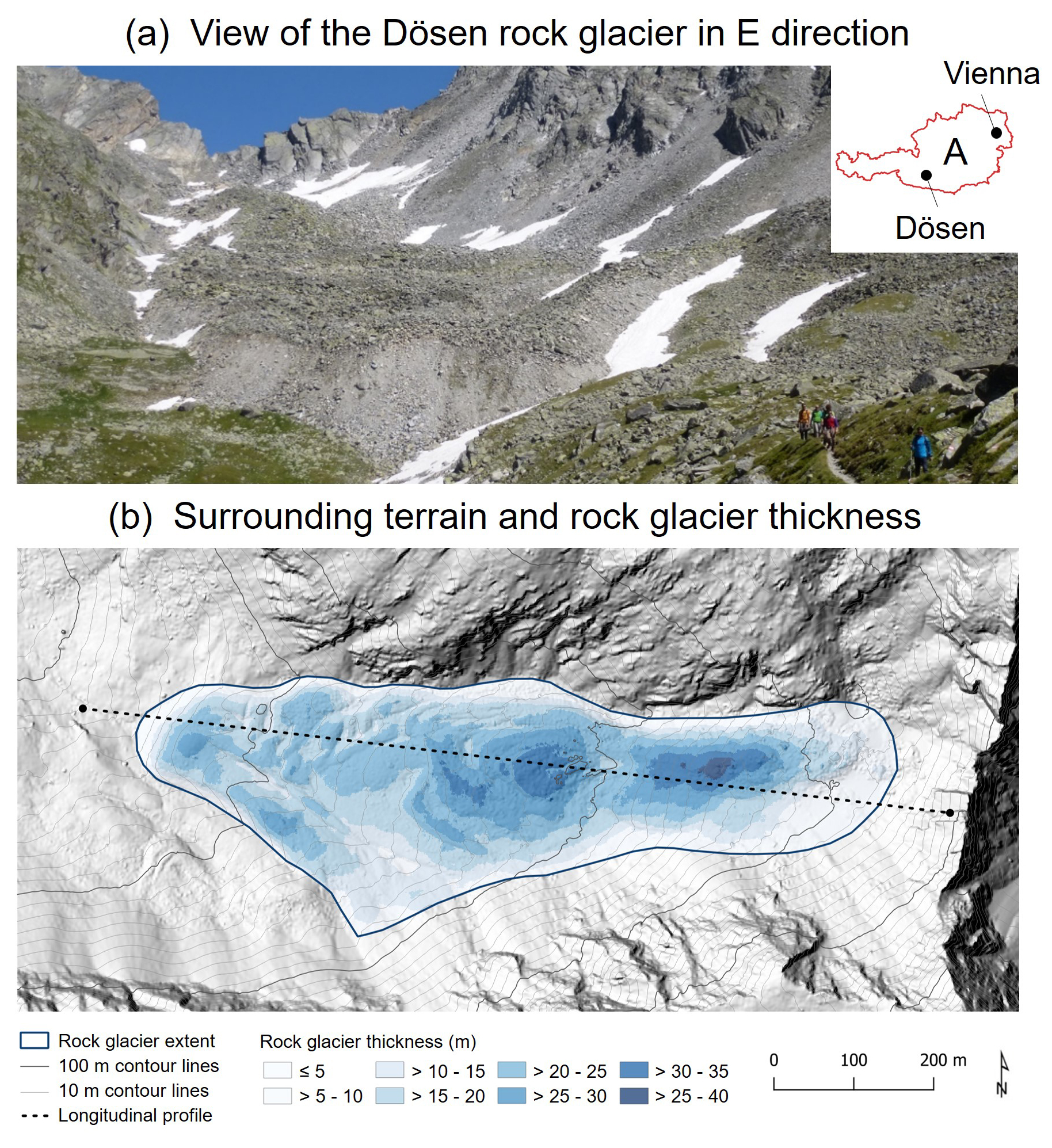
Figure 5 Dösen rock glacier. (a) Location of the rock glacier in Austria and view from the front towards the rooting zone – author: Gerhard K. Lieb; (b) Rock glacier extent and simulation release height, to be understood as the reconstructed thickness of the rock glacier body, based on geophysical evidence and extrapolation (Kellerer-Pirklbauer et al., 2018).

The computational experiment DO1 is applied to a simplified (therefore referred to as semi-generic) representation of the Dösen rock glacier (Fig. 5), using the slow-flow model. The simulation is executed at a raster cell size of 1 m for a duration of 300 years. Table 3 discloses the key parameters, which were calibrated to reach plausible velocities and movement patterns, related to the measurements. Visualization is performed with and without draping of the dynamically adapted orthophoto, in order to additionally analyse the visual effects of the draping.

4 Results

4.1 Generic planar rock slide with interlayer shearing

The equilibrium-of-motion model provides the expected results for the generic planar rock slide, including the formation of back-scarps characteristic for this type of process (Fig. 6). We note that the simulation outcomes are very sensitive to the parameterization, with plausibility strongly depending on the balance between time scaling, ν, and ξ in the equilibrium-of-motion model. Preliminary tests have shown that the result also strongly depends on the raster cell size applied to the simulation. With coarser cell size, numerical diffusion strongly blurs the layer heads, leading to a smoother deformation pattern.

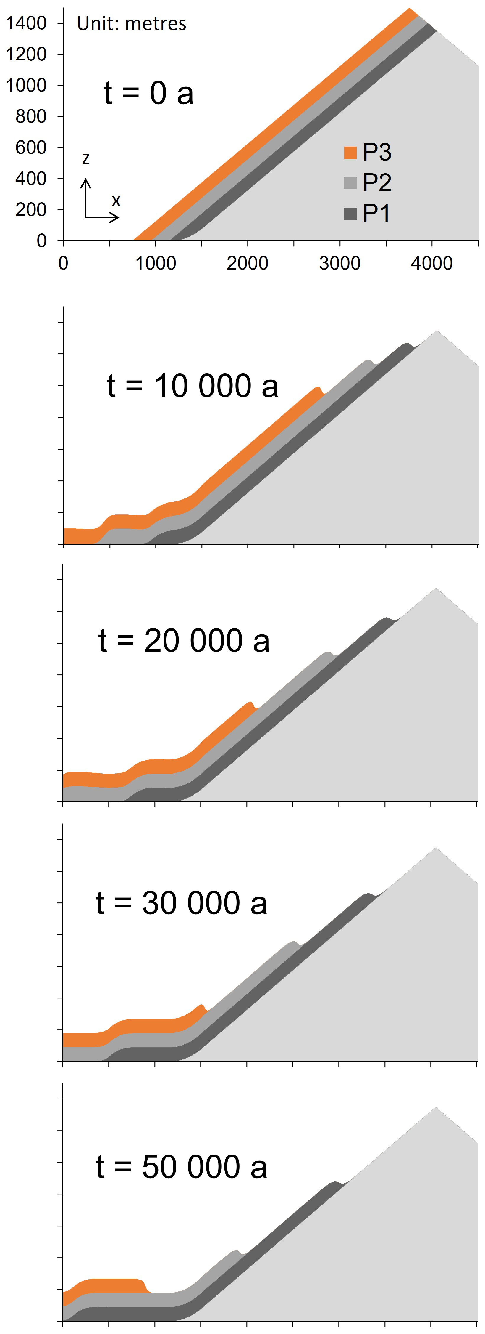
Figure 6 Flow height evolution for the experiment SD1 along a longitudinal profile in down-slope (x) direction, assuming an extremely slow movement.

4.2 Semi-generic Köfels rock slide

Figures 7 and 8 illustrate the differences between the standard r.avaflow model (with one solid phase and full deformation), the one-layer model with controlled deformation, and the two-layer model with controlled deformation. The lower density and therefore larger volume and height of the heavily fractured to crushed rock mass, compared to the release mass, is considered in Figs. 7 and 8: simulated heights are multiplied with a factor up to 1.26, following Zangerl et al. (2021), since the models used in r.avaflow assume a constant density of the material throughout the entire duration of the process.

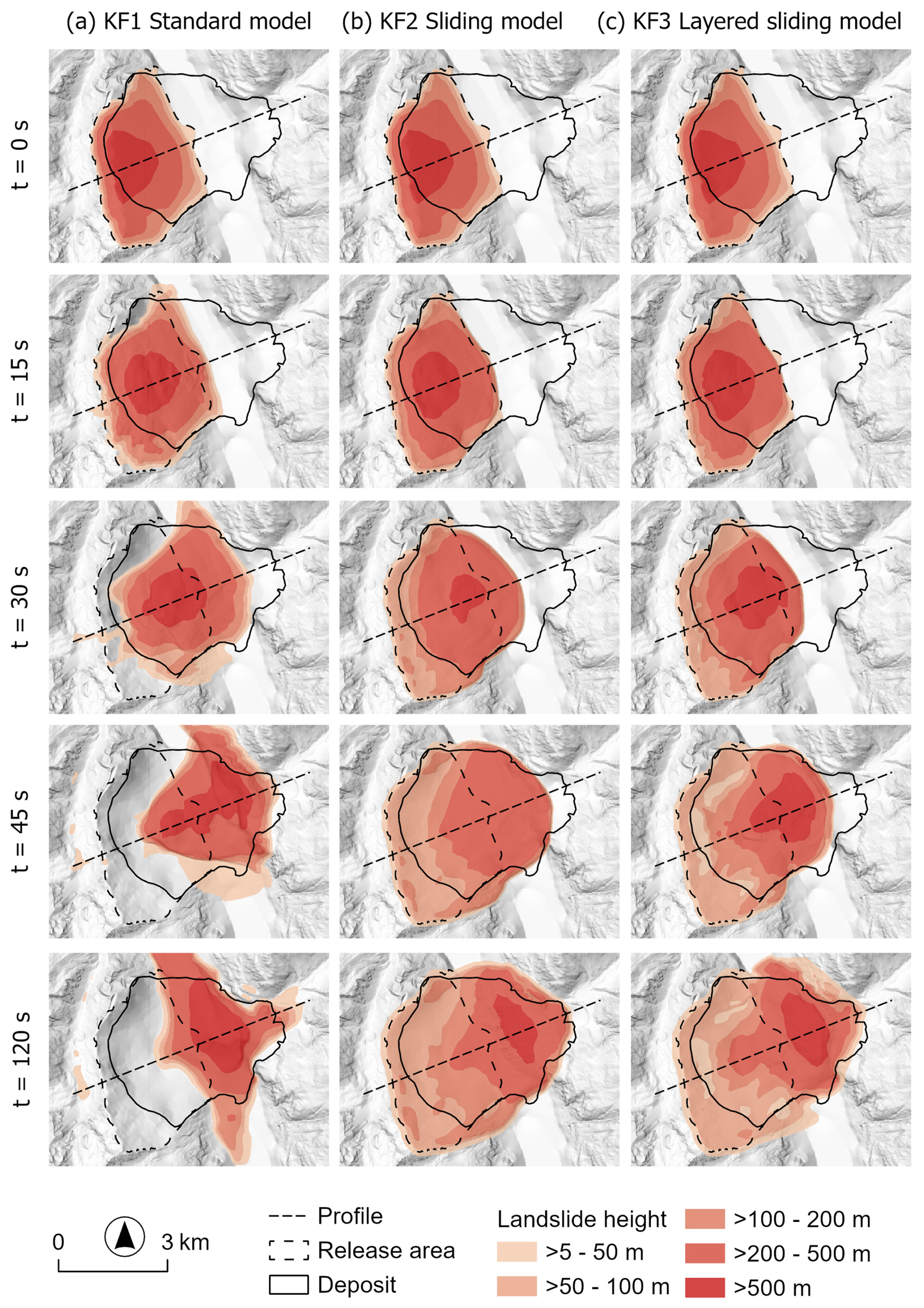
Figure 7 Evolution of flow height for the Köfels experiments KF1–KF3. (a) KF1: standard model without deformation control; (b) KF2: model with one layer, deformation control, and global sliding; (c) KF3: model with two layers, deformation control, and global sliding.

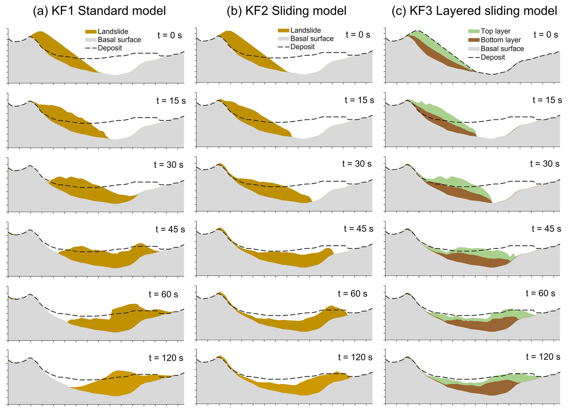
Figure 8 Flow height evolution for the Köfels experiments KF1–KF3 along the longitudinal profile depicted in Fig. 7. (a) KF1: standard model without deformation control; (b) KF2: sliding model with one layer (deformation control and global sliding); (c) KF3: sliding model with two layers (deformation control and global sliding).

With the standard r.avaflow model (experiment KF1), the moving mass displays a strong extension in lateral direction, flowing up and down the Ötz Valley – a behaviour not corresponding to the shape of the observed deposit. This overestimate of lateral spreading is the expected behaviour for a flow model and therefore underlines the call for an approach more adequately representing sliding behaviour. The one-layer model with deformation control (experiment KF2) provides a more realistic representation of the rock slide evolution and deposition. The extent of lateral spreading up and down the Ötz Valley is strongly reduced while the travel distance in sliding direction is in correspondence with the observation (with calibrated parameters). Control of deformation, however, is applied at the cost of a reduced flexibility of the rock mass to adapt to the funnel shape at the outlet of Horlach Valley, so that the front of the simulated rock slide deposit is too wide: the reconstructed impact area is exceeded particularly at the N side (Fig. 7b). Also, the profiles in Fig. 8 reveal that the deposition height is underestimated in the proximal part of the deposition area and overestimated in the distal part. The two-layer model with controlled deformation (experiment KF3) has a strong generic component, as the splitting of the release mass into a top and a bottom layer of equal height is considered due to a lack of more detailed information (Sect. 3.2; Zangerl et al., 2021). The main advantage of the siding surface between the two layers is that the lower layer can entirely deposit in the Ötz valley, whereas the upper layer can slide into the Horlach Valley, to correspond with the observed travel distance of the rock slide. This reduces the need to allow for a very strong deformation of the mass, resulting in a slightly more balanced distribution of the deposit along the flow path, compared to KF2 (Figs. 7 and 8).

In all simulations, process velocities and durations are plausible – considering the displacement of the centre of mass of 2.6 km and a velocity of 50 m s⁻¹ (Erismann et al., 1977), we arrive at a process time of 52 s. Assuming acceleration and deceleration phases, this is in line with the observation that, in all experiments, the mass has almost reached its final position (corresponding to the position at t = 120 s in Figs. 7 and 8) after 60 s.

4.3 Semi-generic East Fogo landslide and tsunami

The evolution of the displacement wave triggered by the semi-generic East Fogo volcanic flank collapse is illustrated in Figs. 9–11, with the standard model and the layered model. Without layering (simulation FO1), the deposition area of the collapsed solid material remains a massive depression until the end of the simulation at t = 900 s. Whilst it is expected that the displacement wave triggered by the impact of the collapse would create such a depression initially, it should be assumed that the restitution of the original sea surface starts soon thereafter – a behaviour which is, however, not reflected in the simulation results. Figure 11 also displays this effect very clearly for the simulation FO1, showing a decrease of the sea level by maximum approx. 980 m for point C1 (Fig. 4), not recovering beyond a level of −900 m until the end of the simulation. A much more realistic behaviour of the system is achieved when applying the layered model (simulation FO2): after an initial positive anomaly caused by the passing of the solid material, the sea level drops to approx. −850 m at the point C1 at about the same time when the minimum is approached in FO1. However, immediately afterwards, the sea level starts to recover, even though some secondary and tertiary waves prevent it from exactly reaching its original state until the end of the simulation. In general, the displacement wave has a much lower magnitude in the simulation FO2 than in the simulation FO1. This phenomenon is most probably related to the different drag concepts used for the standard and layered models and requires some further discussion (Sect. 5). An interesting insight is provided by considering the same landslide with the assumption of a dry ocean basin (Fig. 9a and b). Under such dry conditions there is, as expected, no difference between the simulation results with the standard model and the layered model. When including the ocean water, the landslide becomes less mobile with the standard model (FO1) and, to a much lesser extent, also with the layered model (FO2), due to the decelerating effect of the drag.

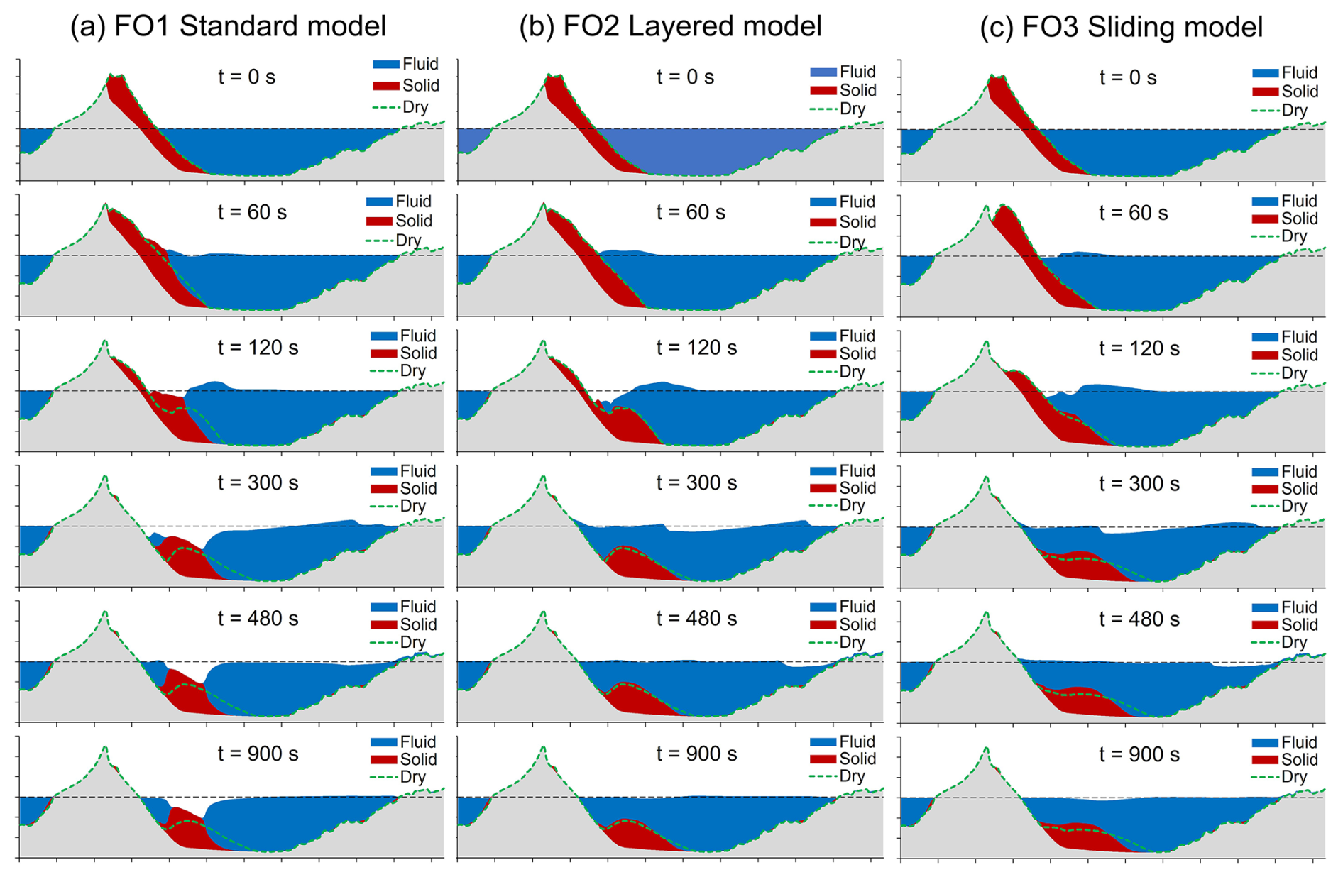
Figure 9 Prehistoric East Fogo event, effects of layering and deformation control on the evolution of flow height until t = 900 s. Sections along profile FOP (Fig. 4b) for the simulations (a) FO1 (standard model); (b) FO2 (layered model); and (c) FO3 (model with deformation control, also referred to as sliding model). Note that the landslide deposit neglecting the interaction with the ocean is included in all profiles, referred to as “Dry”.

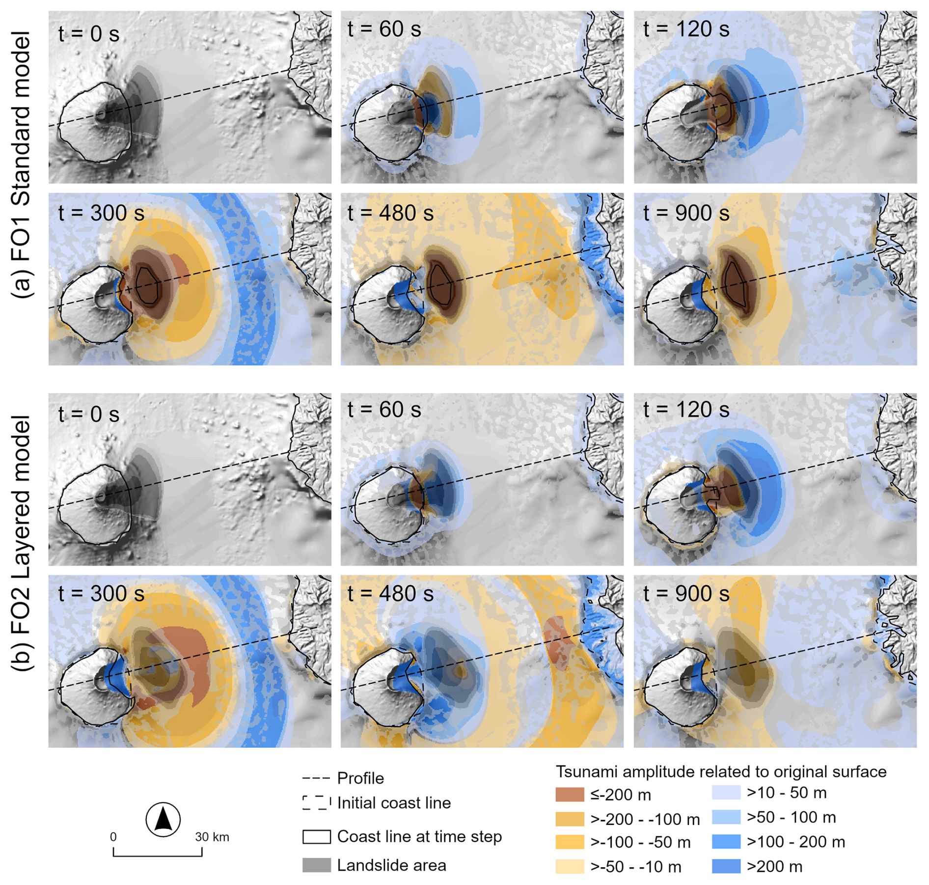
Figure 10 Prehistoric East Fogo event, effects of layering on the evolution of flow height until t = 900 s. Map plots for (a) FO1 and (b) FO2 for selected time steps.

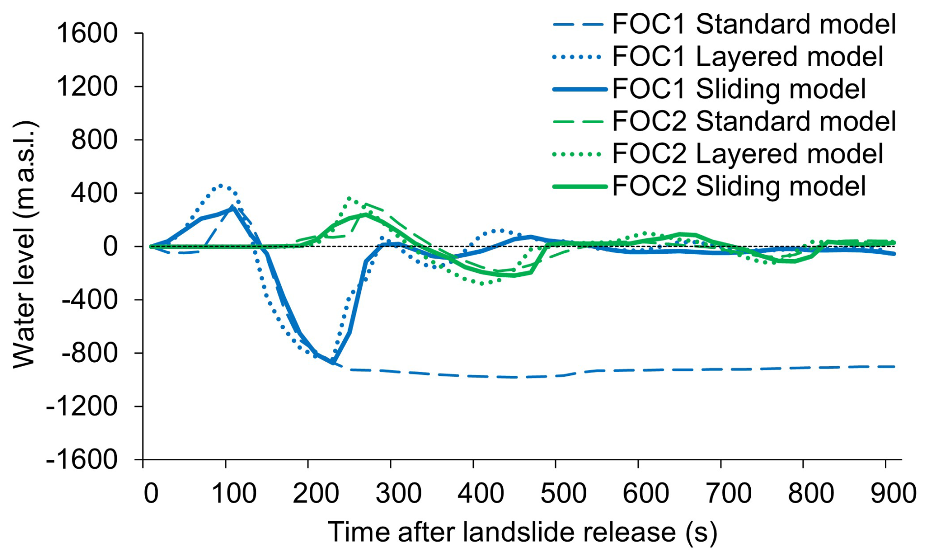
Figure 11 Prehistoric East Fogo event, evolution of the sea surface ($\mathrm{m}\mathrm{a}.\mathrm{s}.\mathrm{l}.$) at the control points C1 and C2 (Fig. 4b) until t = 900 s for the simulations (a) FO1 (standard model), (b) FO2 (layered model), and (c) FO3 (sliding model).

Figure 9c depicts the flow heights for selected time steps as derived with the assumption of a slide-type movement (FO3), applied together with the layered model, whereas the flow height evolution at the points C1 and C2 (Fig. 4b) is illustrated in Fig. 11. There is less compression of the landslide along the down-slope direction with deformation control (sliding model), compared to the other simulations. In the flow models of FO1 and FO2, the internal deformation of the mass is prescribed by its geometry and by topography (Sect. 3.2; Pudasaini and Mergili, 2024a). With the controlled deformation employed in FO3, the mass remains more stretched, mainly because the application of the global gravity components increases acceleration and decreases deceleration in the less steep frontal part, whereas the reverse is the case at the steeper tail. The magnitude of the displacement wave is smaller with FO3, compared to FO2. This phenomenon is most likely a consequence of the higher and steeper front of the flow-type landslide of simulation FO2: both the drag coefficient, as applied in the layered model, and the affected fraction of the water column are comparatively smaller in the case of the slide-type movement of simulation FO3 (Fig. 1b).

4.4 Semi-generic Dösen rock glacier

The simulation on the Dösen rock glacier provides plausible results, with a roughly continuous movement of few decimetres per year (Kaufmann et al., 2007; Kellerer-Pirklbauer and Kaufmann, 2012; Kaufmann, 2016). Figure 12 summarizes the main patterns obtained with the experiment DO1. Figure 12b and c clearly reveal the substantial smoothing effect during the simulation, which are most likely associated with the TVD-NOC numerical scheme applied in r.avaflow (Tai et al., 2002; Wang et al., 2004). This means that the simulation can potentially reproduce or predict the motion of the rock glacier as a whole, whereas the fine-scale movement patterns are lost or at least blurred. In particular, the smaller geomorphological features typical of rock glaciers, such as ridges and furrows, are lost during the 300 year modelling period. For visualization purposes, particularly in the field of science-to-public communication, such fine-scale patterns, representing the morphological characteristics of rock glaciers, are essential to convey rock glacier dynamics and its geomorphic implication. This can be achieved by draping the distorted orthophoto over the rock glacier – fine-scale patterns are preserved in this way, and motion looks much more realistic than with the draped shaded relief map (Fig. 12d).

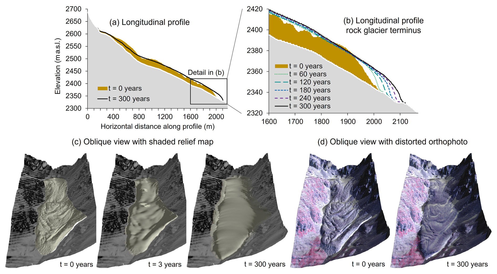
Figure 12 Simulation results for the semi-generic Dösen rock glacier case. (a) Longitudinal profile along the main flow line for t = 0 and t = 300 years including the rock glacier layer based on geophysical data. (b) Longitudinal profile, detail of the rock glacier terminus for six selected time steps. (c) Oblique view against the flow direction, shaded relief map for t = 0, t = 3 years, and t = 300 years. (d) Oblique view with distorted orthophoto for t = 0 and t = 300 years.

5 Discussion

r.avaflow  v4 strongly builds on earlier versions of r.avaflow (first introduced by Mergili et al., 2017), but includes some important enhancements presented in the previous sections. We now discuss the potentials and limitations of these enhancements.

Sliding components have already been included in mass flow models by other authors, such as Bout et al. (2022) who used quite a complex approach, or Cicoira et al. (2022) who employed a full 3D model, which is computationally fairly expensive for complex simulations. To avoid the introduction of a large number of additional, often unknown, parameters and the need for high-performance computers, we decided to introduce a comparatively simple and straightforward approach, based on a mechanical deformation control (Pudasaini and Mergili, 2024a) and on the global gravity components. Figures 6–8 reveal that the model with deformation control introduced in Sect. 2 can be used to produce empirically fairly adequate representations of the prehistoric Köfels rock slide, and plausible results for the generic slope deformation outlined in Sect. 4.1. This indicates that this model might be appropriate for the simulation of slide-type movements. However, it involves some physical, mathematical, and geometric/topographic simplifications, calling for an in-depth discussion of its scope of application and potentials for enhancement and improvement. First, this discussion picks up the complexity versus simplicity discourse regarding landslide modelling, following the hypothesis that simple models with fewer parameters can be preferable for practical application, compared to complex models with many parameters which are often unknown or, even if measurable, have to be calibrated to bring the models in line with the observations. In this sense, the deformation coefficient (Pudasaini and Mergili, 2024a), the fraction of global sliding, or the basal viscosity parameter can be considered either as mechanical or as empirical parameters with some physical background – a description which would, however, also be appropriate for established material parameters such as basal and internal friction, or viscosity. In contrast to established parameters, where a large pool of experiences can be used to choose plausible starting values for parameter optimization procedures and where, with other software packages, even well-established guiding parameter sets are available, the newly introduced values have to be calibrated from scratch. The deformation coefficient and the fraction of global sliding are intuitive quantities, strongly related to obvious characteristics of landslides. However, the time evolution of the model parameters, which can currently be prescribed based on “hard” time steps, relies on prior knowledge of the event. Coupling parameter evolution to dynamic flow characteristics such as velocity gradients could be an interesting future direction, increasing the physical meaning of the model. The possibility to divide the sliding mass into multiple layers, and therefore to define horizons of shearing, increases the flexibility of the model with deformation control. Layering, however, is also important in another context: the simulations on the semi-generic East Fogo event clearly reveal that the standard r.avaflow model is not suitable for those simulations of landslide-to-reservoir impacts where a large landslide body comes to rest at the seafloor without substantial mixing with the water body. The explicit consideration of a layered movement (solid beneath fluid) is appropriate to realistically simulate the restitution of the original water surface (Figs. 9–11). Technically, layering can be implemented in a relatively straightforward way, largely by the adaptation of the gravity components and pressure gradients. A major difference between the standard model and the layered model is the drag. The concept of drag applied by Pudasaini and Mergili (2019) has been developed for mixtures of solid particles and fluid material, but not for layered landslides. The drag concept for layered movements, introduced in Sect. 2.3, represents a rough approximation which is supposed to work best in areas of spatially constant gradients of landslide thickness. Therefore, a direct comparison of the results of the corresponding simulations remains problematic. More research is required in this respect.

The slow-flow model proved to be useful in plausibly reproducing two fundamentally different processes, a three-layer planar rock slide (Fig. 6) and a rock glacier moving downvalley (Fig. 12), A detailed analysis of the correspondence of the empirically optimized viscosity parameters and parameters measured in comparable real-world cases are out of scope here, but the computational experiments reveal an important general limitation of r.avaflow, related to the TVD-NOC numerical scheme: fine-scale geomorphological patterns such as furrows and ridges are smoothed and blurred. For the Dösen rock glacier, we have shown an approach to visually compensate for this issue by distorting the orthophoto, following the direction of motion. A similar approach was demonstrated for the Köfels rock slide, to allow for a more realistic visual impression (cf. Mergili, 2024). A solution to the blurring issue would have to rely on the implementation of a different numerical scheme, which should be a major direction for the future.

Another notable limitation regarding the simulation of large landslides is the application of depth-averaged models, where the height of the landslide should be much lower than the landslide length, and also much lower than the terrain curvature radius. For phenomena such as the Köfels rock slide or the East Fogo event, this condition might be violated, compromising the accuracy of the results. An in-depth benchmark comparison with full 3D models (e.g., Cicoira et al., 2022) would be helpful to learn about the magnitude of those effects. Until more benchmark tests and empirical evaluation efforts will be available, the proposed models should be used with utmost care when it comes to inform hazard zoning, technical protection measures, evacuation strategies, or other measures of “hard” risk management. The models are, however, useful for those purposes where a plausible representation of processes, achieved within short computational times and at high computational efficiency, is more important than high levels of mathematical, physical, and geometric accuracy.

Through the interfaces of r.avaflow  v4 with the 3D visualization and animation software packages Paraview and Blender, and with the game engine Unreal Engine 5, simulation results can be converted into ordinary 3D videos, anaglyph videos, or immersive virtual reality experiences in a straightforward way. Such visually realistic representation of one- or multi-layer slide-type movements over a broad range of time scales and velocities without major computational efforts will be important to feed “gamification” (Pfeffer and Mergili, 2024) to create awareness and interest towards landslides and related phenomena within a broader audience at schools, museums, nature parks, universities, and other relevant social environments.

6 Conclusions

We have equipped the mass flow simulation tool r.avaflow with several additional functions to simulate (i) slide-type landslides with controlled deformation, (ii) layered landslides, and (iii) mass movements which are not extremely rapid. All these enhancements, included in r.avaflow  v4, can be combined for the simulation of single- and multi-layer flow- and slide-type movements which can be extremely rapid to extremely slow. The model with deformation control builds on a small set of empirical parameters with a physical basis and yields plausible results for the test cases of the prehistoric Köfels rock slide and a generic three-layer planar rock slide. For landslide-reservoir interactions, when the mixing between the landslide material and the water body is insignificant, the consideration of a layered movement results in a much more realistic restitution of the pre-event water level after alleviation of the primary displacement wave, compared to the standard multi-phase model used in r.avaflow that assumes phase mixing. Direct comparison between the standard model and the layered model remains a challenge due to different drag concepts to be applied. The slow-flow model proves capable of simulating even very slow movements such as a generic planar rock slide or a slowly downward moving rock glacier in a plausible way. Topographic details of modelled landforms (e.g., furrows and ridges of rock glaciers) are lost for numerical reasons but can be at least visually recreated through draping of a dynamically distorted orthophoto.

The enhanced flexibility of r.avaflow  v4, compared to earlier versions of the software, increases the responsibility of the users to combine terms in a meaningful way. All the extensions introduced, and their interconnection, use simplifications and generalizations, which may lead to the loss of some physical details on the one hand, and a more straightforward parameterization on the other hand. Therefore, these models have to be exposed to additional benchmarking and empirical evaluation with well-documented real-world cases, in order to learn more about the effects of possible limitations of the new functionalities and to constrain suitable parameter values, to become ready for predictive applications in risk management. Furthermore, we plan to implement in a further tool-development step an intelligent warning function to inform users when they enter inappropriate combinations of parameter values. Until then, caution should be exercised when using the proposed models in “hard” risk management contexts, such as early warning systems and spatial planning. Nevertheless, the models represent an important resource for raising awareness and environmental education when used in combination with the newly implemented 3D animation and virtual reality interfaces of r.avaflow  v4.