Development of UI-WRF-Chem (v1.0) for the MAIA satellite mission: case demonstration

The Multi-Angle Imager for Aerosols (MAIA) satellite mission, to be jointly implemented by NASA and the Italian Space Agency, aims to study how different types of particulate matter (PM) pollution affect human health. The investigation will primarily focus on a discrete set of globally distributed Primary Target Areas (PTAs) containing major metropolitan cities, and will integrate satellite observations, ground observations, and chemical transport model (CTM) outputs (meteorology variables and PM concentrations) to generate maps of near-surface total and speciated PM within the PTAs. In addition, the MAIA investigation will provide satellite measurements of aerosols over a set of Secondary Target Areas (STAs), which are useful for studying air quality more broadly. For the CTM, we have developed a Unified Inputs (of initial and boundary conditions) for WRF-Chem (UI-WRF-Chem) modeling framework to support the MAIA satellite mission, building upon the standard WRF-Chem model. The framework includes newly developed modules and major enhancements that aim to improve model simulated meteorology variables, total and speciated PM concentrations as well as AOD. These developments include: (1) application of NASA GEOS FP and MERRA-2 data to provide both meteorological and chemical initial and boundary conditions for performing WRF-Chem simulations at a fine spatial resolution for both forecast and reanalysis modes; (2) application of GLDAS and NLDAS data to constrain surface soil properties such as soil moisture; (3) application of recent available MODIS land data to improve land surface properties such as land cover type; (4) development of a new soil NO_x emission scheme – the Berkeley Dalhousie Iowa Soil NO Parameterization (BDISNP); (5) development of a stand-alone emission preprocessor that ingests both global and regional anthropogenic emission inventories as well as fire emissions.

Here, we illustrate the model improvements enabled by these developments over four target areas: Beijing in China, CHN-Beijing (STA); Rome in Italy, ITA-Rome (PTA); Los Angeles in the U.S., USA-LosAngeles (PTA), and Atlanta in the U.S., USA-Atlanta (PTA). UI-WRF-Chem is configured as 2 nested domains using an outer domain (D1) and inner domain (D2) with 12 and 4 km spatial resolution, respectively. For each target area, we first run a suite of simulations to test the model sensitivity to different physics schemes and then select the optimal combination based on evaluation of model simulated meteorology with ground observations. For the inner domain (D2), we have chosen to turn off the traditional Grell 3D ensemble (G3D) cumulus scheme. We conducted a case study over USA-Atlanta for June 2022 to demonstrate the impacts of the cumulus scheme on precipitation and subsequent total and speciated PM_2.5 concentrations. Our results show that keeping the G3D cumulus scheme turned on results in higher precipitation and lower total and speciated PM_2.5 than the simulation with the G3D cumulus scheme turned off. Compared with surface observations of precipitation and PM_2.5 concentration, the simulation with the G3D scheme off shows better performance. We focus on two dust intrusion events over CHN-Beijing and ITA-Rome, which occurred in March 2018 and June 2023, respectively. We carried out a suite of sensitivity simulations using UI-WRF-Chem by excluding chemical boundary conditions or including MERRA-2 chemical boundary conditions. Our results show that using MERRA-2 data to provide chemical boundary conditions can help improve model simulation of surface PM concentrations and AOD. Some of the target areas have also experienced significant changes in land cover and land use over the past decade. Our case study over CHN-Beijing in July 2018 investigates the impacts of improved land surface properties with recent available MODIS land data on capturing the urban heat island phenomenon. Model-simulated surface skin temperature shows better agreement with MODIS observed land surface temperature. The updated soil NO_x emission scheme in July 2018 also leads to higher NO₂ vertical column density (VCD) in rural areas within the CHN-Beijing target area, which matches better with TROPOMI observed NO₂ VCD. This in turn affects the simulation of surface nitrate concentration. Lastly, we conducted a case study over USA-LosAngeles to tune dust emissions. These examples illustrate the fine-tuning work conducted over each target area for the purpose of evaluating and improving model performance.

1 Introduction

Ambient particulate matter (PM) pollution has been ranked as the top environmental risk factor for premature deaths (Forouzanfar et al., 2016). The integrated use of satellite and chemical transport model (CTM) outputs have shed light on the impacts of PM_2.5 (PM with aerodynamic diameter less than 2.5 µm) on public health in the past decade (Cohen et al., 2017; Wang et al., 2021a). Satellite-retrieved aerosol data products such as aerosol optical depth (AOD) have been widely used to estimate ground-level PM_2.5 concentration over the past two decades (e.g., Shin et al., 2020; Van Donkelaar et al., 2006; Wang and Christopher, 2003) due to the wide spatial coverage achievable from spaceborne observations. Because of uncertainties in remote sensing retrievals and the complex AOD-PM_2.5 relationship (Wang and Christopher, 2003), satellite-derived ground-level PM_2.5 have been combined with ground observations of PM_2.5 and/or CTM simulated PM_2.5 to form a hybrid method of providing a new data source for epidemiological health studies (e.g., Van Donkelaar et al., 2010; Holloway et al., 2021; Diao et al., 2019). This hybrid method has also been used for estimating PM_2.5 component concentration and its application in health-related studies (Philip et al., 2014; Li et al., 2021; Hu et al., 2019; Wei et al., 2023). The association between exposure to PM and mortality has been well established. However, since ambient PM is a complex mixture of particles that vary in size, shape and chemical composition, there remains uncertainty in understanding the relative toxicity of different PM types to human health (Sangkham et al., 2024; Weichenthal et al., 2024).

The Multi-Angle Imager for Aerosols (MAIA) satellite mission to be jointly implemented by the National Aeronautics and Space Administration (NASA) (Diner et al., 2018) and the Italian Space Agency (ASI) has a key objective to map PM composition and study the impacts of different types of PM on human health (Liu and Diner, 2017). The MAIA instrument builds upon the work of the Multi-angle Imaging SpectroRadiometer (MISR) instrument onboard NASA's Terra spacecraft, which has been retrieving aerosol properties including aerosol type since February 2000 (Diner et al., 1998; Kahn et al., 2005). MISR has also been one of the commonly used satellite instruments for mapping global PM concentration for studying air quality and public health (Liu et al., 2009; Holloway et al., 2021; Meng et al., 2018). The MAIA instrument contains a pointable 14-wavelength pushroom camera, spanning the ultraviolet (UV), visible and near-infrared (VNIR) and shortwave infrared (SWIR) regions of the electromagnetic spectrum to measure the spectral radiance of sunlight scattered by the Earth's atmosphere and surface. Three of the bands are polarimetric to further help constrain aerosol particle properties. The MAIA investigation will focus on a globally distributed set of primary target areas (PTAs) (https://maia.jpl.nasa.gov/mission/#target_areas, last access: 7 November 2025) for PM health studies, which include metropolitan cities. For each PTA, it will employ Geostatistical Regression Models (GRMs), to generate maps of surface total PM_2.5, PM₁₀ and speciated PM including sulfate, nitrate, dust, organic carbon (OC) and elemental carbon (EC). The GRMs use satellite retrieved aerosol parameters, CTM outputs (meteorological variables along with total and speciated PM mass concentrations) and other ancillary information such as population density data as predictors. Surface observations of total and speciated PM are used to train the GRMs (i.e., determine the coefficients of the model predictors) (Jin et al., 2024).

Our work here introduces the development of the Unified Inputs (of initial and boundary conditions) for WRF-Chem (UI-WRF-Chem) as the CTM for supporting the MAIA satellite mission, based on the standard WRF-Chem model (Fast et al., 2006; Grell et al., 2005). Since meteorological variables as well as total and speciated PM mass concentrations from UI-WRF-Chem outputs are used in the GRMs to derive the total and speciated PM maps, we have implemented major updates in UI-WRF-Chem that aim to improve model simulated meteorology variables or PM concentration through the integrated use of satellite and ground-based observations. Because WRF-Chem is an online coupled chemical transport model, the improvement of aerosol concentration simulation could also enhance the simulation of meteorology through the incorporation of aerosol radiation feedback, especially in polluted regions such as Delhi, India (Chutia et al., 2024).

The UI-WRF-Chem modeling framework builds upon the standard WRF-Chem model with newly developed modules and major enhancements that enable integration of NASA Goddard Earth Observing System (GEOS) data for unified meteorology and chemistry inputs, updates of land surface properties with recent available Moderate Resolution Imaging Spectroradiometer (MODIS) land data, and expanded emission processing capabilities:

• First, we use the NASA GEOS products including both GEOS Forward Processing (FP) and Modern-Era Retrospective analysis for Research and Application, version 2 (MERRA-2) data to provide both meteorological and chemical initial and boundary conditions for performing WRF-Chem simulation with a finer spatial resolution in forecasting and reanalysis modes, which allows for consistency between meteorology and chemistry. The NASA GEOS system assimilates satellite observations of aerosol products (Randles et al., 2017). Using these assimilated data to provide chemical initial and boundary conditions for WRF-Chem simulations over MAIA target areas would be computationally efficient for capturing long-range or regional transport without enlarging the model domain to include the emission sources. A number of studies have demonstrated the influence of chemical boundary conditions on regional air pollution in the domain of interests, when running WRF-Chem (e.g., Mo et al., 2021; Ukhov et al., 2020; Roozitalab et al., 2021; Wang et al., 2004).

• Second, we employ data from the Global Land Data Assimilation System (GLDAS) (Rodell et al., 2004) or the North American Land Data Assimilation System (NLDAS) (Mitchell et al., 2004) to constrain soil properties such as soil moisture in WRF-Chem. Soil properties are critical for weather forecasts, biogenic emission estimates and dust storm simulation (Han et al., 2021), and ultimately, air quality prediction (Thomas et al., 2019; Jenkins and Diokhane, 2017; de Rosnay et al., 2014). Both GLDAS and NLDAS provide optimized initial soil conditions with a high spatial and temporal resolution for numerical weather forecasting (Dillon et al., 2016; Xia et al., 2014). Better estimates of soil properties also enhance the simulation of soil NO_x emissions, serving as an important part of the total global NO_x budget (Jaeglé et al., 2005), and subsequently improve the simulation of nitrate aerosols.

• Third, we use recent available MODIS land data to update static land surface properties such as land cover type in WRF-Chem. Some of the default land surface properties used in WRF-Chem are out of date. Using recent available MODIS land data to update land surface properties would help improve mesoscale model performances (Li et al., 2014, 2017a; Aegerter et al., 2017; Wang et al., 2023).

• Fourth, we develop the Berkeley Dalhousie Iowa Soil NO Parameterization (BDISNP) scheme for simulating soil NO_x (NO + NO₂) emissions, building upon the Berkeley Dalhousie Soil NO Parameterization (BDSNP) scheme (Hudman et al., 2012). Previous study showed that the default soil NO_x emissions in WRF-Chem could be underestimated by a factor of 10 in some regions (Oikawa et al., 2015). Since soil NO_x emissions play a critical role in the formation of ozone (O₃) and nitrate aerosols (Sha et al., 2021; Lin et al., 2021), their accurate representation in the model is essential.

• Finally, we develop a stand-alone WRF-Chem Emission Preprocessing System (WEPS) that ingests both global and regional anthropogenic emission inventories as well as fire emissions. Because anthropogenic and fire emissions are important for aerosol simulations in the model, building our own emission preprocessor allows us the opportunities to optimize existing emission inventories and add new ones, including those from top-down estimates (Wang et al., 2020b, c).

In this paper, we present the developments of the UI-WRF-Chem modeling framework and illustrate the resulting model improvements. We focus on four target areas, three of which are MAIA PTAs: Rome, Italy (ITA-Rome), Los Angeles, California (USA-LosAngeles) and Atlanta, Georgia (USA-Atlanta). We also include Beijing, China (CHN-Beijing), which is MAIA secondary target areas (STAs). STAs are regions that will be observed by the MAIA satellite instrument but not necessarily processed to the same level as PTAs. These four target areas together provide a good representation of the range of PM pollution levels from low (Los Angeles and Atlanta), to high (Beijing) with Rome in the middle. Some of our previous studies have focused on other MAIA PTAs using the UI-WRF-Chem modeling framework. Li et al. (2024) developed an inverse modeling method to improve the diurnal profile of anthropogenic emissions in the Addis Ababa, Ethiopia PTA, using surface-based PM observations from both U.S. Embassy sites and PurpleAir sensors. Chutia et al. (2024) investigated the impacts of aerosol-radiation interaction on air quality in the Delhi, India PTA. Overall, current work along with previous work can provide a good picture of the model performance for different applications. This paper is organized as follows: Sect. 2 focuses on the description of the UI-WRF-Chem model development; Sect. 3 provides the model configuration used in the target areas; Sect. 4 analyzes the case studies for different target areas; and Sect. 5 presents conclusions and discussion.

2 UI-WRF-Chem development

In this section, we first provide a brief overview of the MAIA PM products to illustrate the role of UI-WRF-Chem. We then describe the development of the UI-WRF-Chem modeling framework, emphasizing the major updates and key components designed to address the needs of the MAIA satellite mission.

2.1 Overview of MAIA PM products

The MAIA PM products to be generated in the PTAs include a Level 2 (L2) PM product and a Level 4 (L4) Gap-Filled PM (GFPM) product. Both L2 and L4 PM products include 24 h averaged total and speciated PM mass concentration with a spatial resolution of 1 km within bounding boxes measuring 360 km × 480 km (east-west × north-south) size. The L2 PM data are only available for days corresponding to MAIA satellite overpasses (typically 3–4 times per week in the PTAs) at locations with valid MAIA aerosol retrievals. The L4 PM data merge L2 satellite-derived PM concentration with bias-corrected PM concentrations from UI-WRF-Chem outputs and are therefore spatially (covering the whole target area) and temporally (daily) “complete”. The L2 PM product is derived using GRMs which take the satellite retrieved aerosol parameters, meteorological variables and total and speciated PM concentrations from UI-WRF-Chem and other ancillary information such as population density data as predictors and surface observations of total and speciated PM concentrations as target variables. GRMs are trained for each PM type and each PTA. For the launch-ready version of the GRMs, four meteorological variables from UI-WRF-Chem are used: 2 m air temperature, 10 m wind speed, surface relative humidity (RH) and planetary boundary layer height (PBLH). To generate the L4 GFPM product, separately trained GRMs are employed to generate a bias-corrected, CTM-based PM product where the primary predictor is the CTM-generated PM concentration, rather than the satellite-retrieved aerosol optical depth. Other predictors and target variables are the same as those used in the generation of L2 PM product. For areas where both satellite-derived L2 PM and CTM-based PM products are available, these two products are then combined using weights derived from a Bayesian Ensemble Averaging model to generate the final L4 GFPM product. More detailed information can be found in Jin et al. (2024).

Two versions of the MAIA L2 PM and L4 GFPM products will be generated as part of the routine processing: the “forecast” and the “reanalysis” version. For the forecast product version, GEOS FP meteorology is used for model initial and boundary conditions and GEOS FP fields of aerosols and aerosol precursors will also be used to specify boundary conditions of atmospheric composition. The reanalysis versions replace GEOS FP variables with outputs from MERRA-2 data. Due to the ∼ 6 month latency of speciated PM_2.5 data from surface monitors, the forecast versions will rely on previously available measurements. Generation of the reanalysis products will nominally occur on an annual basis and will benefit from more complete surface monitor datasets. More detailed information about the PM products can be found at https://maia.jpl.nasa.gov/resources/data-and-applications/ (last access: 7 November 2025).

2.2 Overview of UI-WRF-Chem modeling framework

To meet these needs, UI-WRF-Chem is designed to operate in both forecasting (or near real time, NRT) and reanalysis modes. We use the NASA GEOS model data: GEOS FP in forecasting or NRT mode and MERRA-2 in reanalysis mode to drive WRF-Chem simulations by providing self-consistent and unified meteorological and chemical initial and boundary conditions, referred to as the Unified Inputs (of initial and boundary conditions) for meteorology and chemistry. Figure 1 presents the flowchart of the UI-WRF-Chem modeling framework. Here, we provide a brief description of the UI-WRF-Chem framework, outline the components included in the standard WRF-Chem model and highlight the major updates we have introduced.

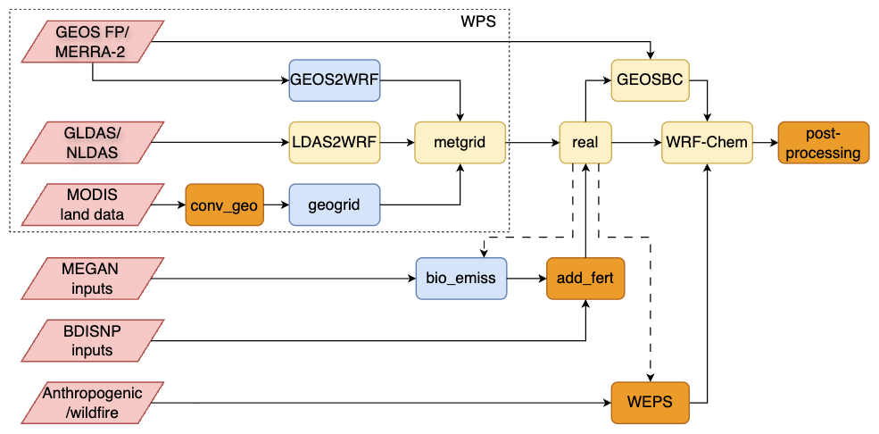
Figure 1 Flowchart of UI-WRF-Chem modeling framework. Pink parallelogram represent input datasets used, including meteorological, land surface and emission data. Rounded rectangles represent different modules and processes within the UI-WRF-Chem framework. Blue rounded rectangles denote standard WRF-Chem components without any changes, except for GEOS2WRF, which is from NASA's NU-WRF framework. Yellow round rectangles represent modified modules based on standard WRF-Chem components, except for LDAS2WRF, which is adapted from GEOS2WRF. Orange rounded rectangles indicate new modules developed in this work. The input datasets and modules enclosed within the dashed box corresponds to the WPS in the standard WRF-Chem model, where meteorological files (met_em.d*.nc) are generated. The conv_geo process converts MODIS land data into binary files, for the geogrid process. Both GEOS2WRF and LDAS2WRF convert input data in the NetCDF file format to an intermediate file format, equivalent to the ungrib process. GEOSBC is adapted from the mozbc module, where GEOS FP and MERRA-2 data are used to update chemical initial and boundary conditions. The bio_emiss module reads MEGAN emission input datasets (e.g., isoprene emission factor) and generates files (wrfbiochemi_d0*) for WRF-Chem to calculate biogenic emissions. The add_fert module is used to add the BDISNP input datasets (e.g., fertilizer data) into the wrfbiochemi_d0* files for the real process. WEPS processes both anthropogenic and fire emission datasets and converts them into WRF-Chem ready emission files (*wrfchemi*). Dashed lines from real to bio_emiss and WEPS indicate that real needs to be executed once before running the full flow to generate wrfinput_d0* files, which provide domain information to these two modules.

Compared with the standard WRF-Chem model, the UI-WRF-Chem modeling framework incorporates new modules and significant modifications to enable the seamless use of NASA GEOS data, updates of land surface properties with recent available MODIS land data and expanded emission capabilities. First, we incorporate the GEOS2WRF module from NASA's Unified-Weather Research and Forecasting model (NU-WRF) (Peters-Lidard et al., 2015), which functions similarly to the standard ungrib process, by converting GEOS FP or MERRA-2 data to an intermediate file format. We also develop the LDAS2WRF module, adapted from the GEOS2WRF module to convert the GLDAS or NLDAS data into the same intermediate file format. The standard metgrid process then converts these intermediate files into meteorological files in the NetCDF format (met_em.d*.nc), respectively. These two NetCDF files are subsequently merged to generate the final meteorological files for the real process. Second, to integrate the MODIS land data into the static geographical datasets, we develop the conv_geo Python-based module, where we convert the MODIS land data into the standard binary file formats required by the geogrid process. This enables updates of land surface properties with recent available MODIS land data, not available in the standard WRF-Chem model. We also develop the GEOSBC module, by modifying the standard mozbc module to use GEOS FP or MERRA-2 data for updating both chemical initial and boundary conditions, which improves the consistency between meteorology and chemistry inputs. Additionally, we modify WRF-Chem's chemistry scheme to ensure compatibility between dust fields from GEOS FP or MERRA-2 and the dust representation in the chemistry scheme itself (see Sect. 2.7 for more information).

For emissions, we develop the BDISNP scheme for soil NO_x emissions by extending the workflow of the standard MEGAN-based biogenic VOC calculation. Same as the MEGAN process, we first use the standard bio_emiss module to read the MEGAN emission input datasets (e.g., isoprene emission factor) and then convert them into the wrfbiochemi_d0* files for the real process. We then apply the add_fert module that we have developed here to incorporate emission input datasets (e.g., fertilizer data), specific to the BDISNP scheme into wrfbiochemi_d0* files. Additionally, we modify WRF-Chem codes to calculate soil NO_x emissions. We also develop the WEPS module to process both anthropogenic and fire emissions, adopting some functionalities from the widely used anthro_emiss and EPA_ANTHRO_EMISS utilities in the WRF-Chem community. This provides flexibility for incorporating additional emission inventories into the WEPS. Lastly, we develop a Python-based postprocessing module to calculate selected WRF-Chem variables and compile hourly WRF-Chem output files into daily files in the formats required by the GRMs.

2.3 Updates of meteorological and chemical initial and boundary conditions as well as soil properties

Here, we have adopted the functionality of the NASA's NU-WRF to drive WRF-Chem by providing unified meteorological and chemical initial and boundary conditions using GEOS FP and MERRA-2 data. Both GEOS FP and MERRA-2 data are generated within the GEOS atmospheric and data assimilation system (Rienecker et al., 2008), in which meteorological and aerosol observations are jointly assimilated. GEOS FP uses the most recent GEOS system to produce the real-time forecasting data while MERRA-2 uses a frozen version of the GEOS system to conduct the long-term atmospheric reanalysis since 1980. The GEOS native model is on a cubed sphere grid with 72 hybrid-eta layers from surface to 0.01 hPa. Products are saved on a 0.5° × 0.625° latitude by longitude grid for MERRA-2 and 0.25° × 0.3125° latitude by longitude for GEOS FP (Gelaro et al., 2017).

MERRA-2 assimilates multiple streams of aerosol products including bias corrected AOD calculated from observed radiances measured by the Advanced Very High Resolution Radiometer (AVHRR) over ocean prior to 2002 and by MODIS on Terra and Aqua satellites over dark surfaces and ocean since 2000 and 2002, respectively; also assimilated are the MISR AOD over bright land surface and AOD measurements from Aerosol Robotic Network (AERONET) before 2014 (Randles et al., 2017). In the NRT mode, GEOS FP only assimilates AOD derived from MODIS Terra and Aqua. The aerosol module used in the GEOS system is the Goddard Chemistry, Aerosol, Radiation, and Transport (GOCART) model (Colarco et al., 2010; Chin et al., 2002). The GOCART module simulates major aerosol species including sulfate, BC, OC, dust (five bins with lower and upper radius range as: 0.1–1, 1–1.8, 1.8–3, 3–6, 6–10 µm), and sea salt (five bins with lower and upper radius range as: 0.03–0.1, 0.1–0.5, 0.5–1.5, 1.5–5.0, 5.0–10 µm). These aerosol products are available in both GEOS FP and MERRA-2 products. Since 2017, nitrate aerosols have been added into the GEOS system and GEOS FP products thus include nitrate aerosols.

Our work differs from the past work that uses the GEOS FP or MERRA-2 data to drive WRF-Chem in several aspects. For example, Peters-Lidard et al. (2015) presented the NU-WRF model that can be driven by GEOS FP and MERRA-2, but its atmospheric chemistry process is simplified with the GOCART module (without prognostic simulation of aerosol size distribution and nitrate for example) and is designed to be an observation driven integrated modeling system that represents aerosol, cloud, precipitation, and land processes at satellite-resolved scales (∼ 1–25 km). Hence, its real-time application for atmospheric chemistry and aerosol composition forecast is rather limited. Nevertheless, the NU-WRF's concept and framework (GEOS2WRF, Fig. 1) of using GEOS FP and MERRA-2 to drive WRF-Chem are adopted by UI-WRF-Chem development here to provide meteorological initial and boundary conditions for WRF-Chem, using meteorological variables other than soil properties.

Adopting of GEOS FP or MERRA-2 soil properties into WRF-Chem needs special treatment. In the GEOS system, the land surface model (LSM) is a catchment-based model (Koster et al., 2000), which is fundamentally different from the LSMs available in WRF-Chem. The commonly used LSMs in WRF-Chem include the Noah scheme (Chen et al., 1996; Chen and Dudhia, 2001), the Rapid Update Cycle (RUC) (Smirnova et al., 2000), and the Community Land Model (CLM) (Oleson et al., 2004), which are all column-based models with different soil layers. To resolve this issue, Peters-Lidard et al. (2015) used the Land Information System (LIS) (Kumar et al., 2006) to process GEOS outputs and provide initial conditions of soil properties such as soil temperature and soil moisture for running WRF and NU-WRF (Kumar et al., 2008). Since land surface process is slow and usually requires years of LIS simulation to stabilize the soil properties in the model, we have here developed a module (LDAS2WRF, Fig. 1) to utilize soil data products from two land data assimilation systems, GLDAS (Rodell et al., 2004) and NLDAS (Mitchell et al., 2004), which use LIS to focus on the analysis of soil properties in near real time. This way, we reduce the computational cost and complexity of running LIS within the UI-WRF-Chem. The initial conditions of soil properties can have an important impact on boundary layer processes for days to weeks (the so-called memory effect). Hence, the special treatment of soil properties by using observation-constrained GLDAS and NLDAS in UI-WRF-Chem is warranted.

We have developed the capability to use GEOS FP and MERRA-2 data to provide chemical initial and boundary conditions in our UI-WRF-Chem modeling framework. Since WRF-Chem is a regional chemical transport model, time-varying chemical boundary conditions from global chemical transport models are typically used to specify concentrations of different chemical species at the domain boundaries. This is especially important for long-lived chemical species, such as O₃, or capturing regional or long-range transport events. The common practice is to use global model outputs such as the Community Atmosphere Model with Chemistry, CAM-Chem (Emmons et al., 2020) for reanalysis or the Whole Atmosphere Community Climate Model (WACCM) (Gettelman et al., 2019) for forecasts. Unlike CAM-Chem or WACCM, which do not assimilate satellite aerosol observations, GEOS FP and MERRA-2 incorporate satellite-based aerosol data assimilation, which provides observational constraints for the day-to-day variations in aerosol concentrations over a given domain. To leverage this unique capability, we have modified the WRF-Chem preprocessor tool – mozbc (https://www2.acom.ucar.edu/wrf-chem/wrf-chem-tools-community, last access: 10 May 2022) to create the GEOSBC module (Fig. 1), enabling direct ingestion of GEOS FP and MERRA-2 data for updating chemical initial and boundary conditions.

Lastly, we have developed a method to constrain the chemical boundary condition for the allocation of dust concentration in the MERRA-2 data as a function of different dust size bins. While assimilating satellite-derived aerosol optical parameters can improve the simulation of dust in MERRA-2 data, uncertainties remain in simulating the dust size distribution from emission sources and along the transport pathway in the MERRA-2 data (Kramer et al., 2020). These uncertainties are particularly evident during long-range dust transport events, due to factors such as the deposition process and the quality of satellite data being assimilated (Zhu et al., 2025). To address this, we have developed a method to further constrain the MERRA-2 simulated dust size distribution with AERONET observation, which can be incorporated into the chemical boundary conditions for simulating the impacts of dust transport on the domain of interest. This method is applicable in regions where AERONET sites with long-term data are available. We compare the dust particle size distribution (PSD) from MERRA-2 data with AERONET observations to improve the allocation of dust concentration into different size bins in the chemical boundary conditions. A detailed description and application of this approach are provided in Sect. 4.1 and 4.2.

2.4 Updates of land surface properties

We develop capabilities within UI-WRF-Chem to update land surface properties using recent available satellite-based land data products through the WRF Preprocessing System (WPS). MODIS land products are applied here to update four key land surface properties in the Noah LSM: land cover type on an annual basis and green vegetation fraction (GVF), leaf area index (LAI), and surface albedo on a monthly basis. These variables are among the key surface properties in the land model that regulate the exchanges of energy, water, and momentum (Mölders, 2001). The major technical development and its application to study the impacts of land use/cover changes on urban temperature in Eastern China during 2003–2019 were described in Wang et al. (2023). Below we briefly describe the updates of each land surface property.

The standard WRF-Chem model provides different sources of data for land surface properties. For land cover type, one data source is from the U.S. Geological Survey (USGS) map with 24 land cover types, which is derived from the monthly AVHRR Normalized Difference Vegetation Index (NDVI) observations from April 1992 to March 1993. Another one is from the MODIS land cover data including 17 land cover types, based on the International Geosphere-Biosphere Program (IGBP) scheme (Friedl et al., 2002) and three classes of tundra (Justice et al., 2002). Historically, MODIS land cover data inputs used in WRF-Chem have been fixed to years such as 2001 or 2004, or to 2001–2010 climatology data (Broxton et al., 2014). For GVF, the default data is derived from the AVHRR NDVI observations (1985–1990). An alternative option is to use the MODIS Fraction of Photosynthetically Active Radiation (FPAR) (early 2000s) to substitute for GVF. For LAI and surface albedo, one option is to calculate the values online using a look-up table, based on each land cover type. Another option is to use the MODIS LAI and albedo data directly (early 2000s).

Since these data sources are outdated, we have developed the conv_geo Python-based module (Fig. 1) to update all four land surface properties in UI-WRF-Chem via the WPS using recent available MODIS land data. This approach provides self-consistence among the key land surface properties used in the land model as they come from the same satellite observations and offers a flexible way to apply the data for WRF-Chem simulations across different spatial resolutions. Specifically, the land cover type is updated with the MODIS yearly land cover type product (MCD12Q1). GVF can be updated by: (1) deriving from the MODIS monthly NDVI product (MOD13A3) or (2) substituting with MODIS 8-day FPAR product (MCD15A2H). LAI is updated directly from MODIS 8-day LAI product (MCD15A2H). Surface albedo can be updated using either the MCD43A3 daily albedo product or the MODIS combined Terra and Aqua Bidirectional Reflectance Distribution Function (BRDF) and Albedo daily product (MCD43C3). For the MAIA project, MODIS land data from 2018–2020 are used as static inputs to the UI-WRF-Chem simulations, except for CHN-Beijing where only 2018 data are applied.

2.5 Development of the BDISNP soil NO_x emission scheme

The new BDISNP soil NO_x emission scheme is also integrated as part of the UI-WRF-Chem framework. The detailed development of the scheme has been described in Sha et al. (2021) and Wang et al. (2021c). Briefly, in the standard WRF-Chem model, soil NO_x emissions are calculated using the Model of Emissions of Gases and Aerosols from Nature (MEGAN) (Guenther et al., 2006; Guenther et al., 2012), which is intended for estimating biogenic emissions of volatile organic compounds (VOCs). In the MEGAN model, emission factors are based on four global plant function types (broadleaf trees, needleleaf trees, shrubs/bushes and herbs/crops/grasses). Previous work by Oikawa et al. (2015) has suggested that soil NO_x emissions calculated from the MEGAN model using WRF-Chem can be a factor of 10 underestimated in the Imperial Valley, California, compared with ground observations. The BDSNP soil NO_x emission scheme, currently implemented in the global 3-D GEOS-Chem model (Hudman et al., 2012), was added into the UI-WRF-Chem, as the BDISNP, with several of our own updates.

As in BDSNP, the BDISNP includes a more physical representation of the soil NO_x emission process compared with the MEGAN model. The BDISNP considers available nitrogen (N) in soils from biome specific emission factors, online dry and wet deposition of N, and fertilizer and manure N. It also includes the pulsing of soil NO_x emission following soil wetting by rain and the impacts of soil temperature and moisture. Compared to BDSNP, we have made four major updates in the BDISNP: (1) updating the land cover type data with the recent available MODIS land cover type data to better reflect the land cover change; (2) using the GLDAS soil temperature data for calculating soil NO_x emissions rather than using the 2 m air temperature as a proxy for soil temperature; (3) using the modeled GVF data to determine the distribution of arid and non-arid regions to replace the static climate data used in the BDSNP scheme. With these three updates, Sha et al. (2021) has shown that the WRF-Chem simulation with the BDISNP scheme leads to a better agreement with TROPOspheric Monitoring Instrument (TROPOMI) retrieved NO₂ columns over California for July 2018, compared with using the default MEGAN scheme. The increased soil NO_x emissions with the BDISNP scheme result in a 34.7 % increase in monthly mean NO₂ columns and 176.5 % increase in surface NO₂ concentration, which causes an additional 23.0 % increase in surface O₃ concentration in California. The work of Zhu et al. (2023) used derived soil NO_x flux measurements from a field campaign over the San Joaquin Valley in California during June 2021 to evaluate three soil NO_x emission schemes: the MEGAN in the California Air Resource Board (CARB) emission inventory, the Biogenic Emission Inventory System (BEIS) and the BDISNP developed here. It was found that both MEGAN and BEIS inventories were lower than the observation by more than one order of magnitude, and the BDISNP was lower by a factor of 2.2. Even though being underestimated, the BDISNP and the observation showed a similar spatial pattern and temperature dependence.

The fourth update revises the default soil temperature response function in the BDSNP scheme, as described in Wang et al. (2021c). In the default scheme, the soil temperature response follows an exponential function for soil temperature between 0 and 30 °C and stays the same as 30 °C after the soil temperature is above 30 °C. In the work of Oikawa et al. (2015), which found high soil NO_x emissions in high-temperature agricultural soils, an observation-based soil temperature response function was developed. This function is used here to update the default soil temperature response function. Specifically, for soil temperature in the range of 20 and 40 °C, it is a cubic function of soil temperature. When soil temperature is greater than 40 °C, the value of the response function is set the same as the value of soil temperature at 40 °C. In addition, final soil NO_x emissions are reduced by 50 % following the work of Silvern et al. (2019) and Vinken et al. (2014). With this update, Wang et al. (2021c) showed that the GEOS-Chem simulated tropospheric NO₂ vertical column density (VCD) agrees better with Ozone Monitoring Instrument (OMI) observed NO₂ VCD for 2005–2019 summer in the U.S., compared with the GEOS-Chem simulation that uses the default soil temperature function. This model improvement further helps explain the slowdown of tropospheric NO₂ VCD reduction during 2009–2019 observed by OMI in the U.S.

2.6 Development of WRF-Chem Emission Preprocessing System (WEPS)

The WEPS Fortran utility is developed to map both global and regional anthropogenic emissions as well as fire emissions for running UI-WRF-Chem simulations. WEPS builds upon a few tools used in the WRF-Chem community (https://www2.acom.ucar.edu/wrf-chem/wrf-chem-tools-community, last access: 10 May 2022). For example, the anthro-emiss utility creates WRF-Chem ready emission files from global anthropogenic emission inventory datasets. There is also another Fortran program (emission_v3.F) to process the U.S. EPA National Emissions Inventory (NEI) 2005 and 2011. Recently, a new tool EPA_ANTHRO_EMIS has been developed to create WRF-Chem ready anthropogenic emission files from Sparse Matrix Operator Kernel Emissions (SMOKE) Modeling System netcdf outputs for NEI 2014 and 2017. We have adopted some of the functionalities in these tools into the WEPS.

Currently in WEPS, we can ingest the following global anthropogenic emission inventories: (1) HTAP_v2.2 (Janssens-Maenhout et al., 2015) and HTAP_v3 (Crippa et al., 2023), created under the umbrella of the Task Force on Hemispheric Transport of Air Pollution (TF HTAP), which is the compilation of different emission inventories over specific regions (North America, Europe, Asia including Japan and South Korea) with the independent Emissions Database for Global Atmospheric Research (EDGAR) inventory filling in for the rest of the world; (2) EDGARv5.0 for year 2015 (Crippa et al., 2020). The HTAP_v3 includes regional emission inventories from U.S. EPA NEI, CAMS-REGv5.1 for Europe, the Regional Emission inventory in Asia (REASv3.2.1), the Clean Air Policy Support System (CAPSS-KU) inventory over South Korea, the JAPAN emission inventory (PM2.5EI and J-STREAM) in Japan and EDGARv6.1 (https://data.jrc.ec.europa.eu/dataset/df521e05-6a3b-461c-965a-b703fb62313e, last access: 1 December 2023) for the rest of the world. It consists of 0.1° × 0.1° grid maps of species: CO, SO₂, NO_x, non-methane volatile organic compound (NMVOC), NH₃, PM₁₀, PM_2.5, BC and OC for year 2000–2018 (Crippa et al., 2023). Four sectors are included for these species: energy (mainly power industry), industry (manufacturing, mining, metal, cement, etc.), transport (ground transport such as road) and residential (heating/cooling of buildings etc.). For NH₃, an additional sector – agriculture is also included. The datasets have a monthly temporal resolution, and we have interpolated them to daily data. In addition, we have added sector-based diurnal profiles, following the work of Du et al. (2020). For UI-WRF-Chem simulation over the U.S. domain or China domain, we have added the capability to use U.S. EPA NEI 2017 or the Multi-resolution Emission Inventory model for Climate and air pollution research (MEIC) (Zheng et al., 2018; Li et al., 2017b) emission inventory to replace the global emission inventory HTAP_v3, respectively.

For fire emissions, the WEPS can process several emission inventories as described in Zhang et al. (2014). They include: Fire Locating and Modeling of Burning Emissions inventory (FLAMBE) (Reid et al., 2009); Fire INventory from NCAR version 1.0 (FINN v1.01) (Wiedinmyer et al., 2011); Global Fire Emission Database version 3.1 (GFED v3.1) (van der Werf et al., 2010); Fire Energetics and Emissions Research version 1.0 using fire radiative power (FRP) measurements from the geostationary Meteosat Spinning Enhanced Visible and Infrared Imager (FEER-SEVIRI v1.0) (Roberts and Wooster, 2008; Ichoku and Ellison, 2014); Global Fire Assimilation System (GFAS v1.0) (Kaiser et al., 2012); NESDIS Global Biomass Burning Emissions Product (GBBEP-Geo) (Zhang et al., 2012); Quick Fire Emissions Dataset version 2.4 (QFED v2.4) (Darmenov and Da Silva, 2015). Our recent work involves developing a Visible Infrared Imaging Radiometer Suite (VIIRS) based fire emission inventory, FIre Light Detection Algorithm (FILDA-2) (Zhou et al., 2023). Our past work has mainly focused on OC and BC emissions from the FLAMBE emission inventory (e.g., Ge et al., 2014; Zhang et al., 2022, 2020). We have now included gas species such as CO from FLAMBE emission inventory. The injection height by default is set to range from 500 to 1200 m, based on our previous work (e.g., Yang et al., 2013; Wang et al., 2013; Ge et al., 2017) and users have the option to specify the injection height on their own.

2.7 Updates of WRF-Chem chemistry scheme

The MAIA investigation not only focuses on the total PM_2.5 and PM₁₀ mass but the speciated PM_2.5 including sulfate, nitrate, BC or EC, OC and dust. We have therefore selected the Regional Acid Deposition Model, Version 2 (RADM2) for gas-phase chemistry (Stockwell et al., 1990) and the Modal Aerosol Dynamics model for Europe (MADE) (Ackermann et al., 1998) and the Secondary ORGanic Aerosol Model (SORGAM) (Schell et al., 2001) as the aerosol module for MAIA model simulations, using WRF-Chem Version 3.8.1. The RADM2-MADE/SORGAM chemistry mechanism in WRF-Chem simulates the above-mentioned aerosol species and has been widely used to study air quality (e.g., Georgiou et al., 2018; Zhang et al., 2020; Tuccella et al., 2012). The MADE/SORGAM aerosol module also includes ammonium, sea salt and water. The aerosol size distribution is represented by the modal approach (Binkowski and Shankar, 1995), which uses three modes (the Aitken, accumulation and coarse mode). A log-normal size distribution and internal mixing of aerosol species are assumed in each mode.

In the MADE/SORGAM aerosol scheme, dust is not explicitly simulated but rather blended into other species. For smaller size bins of dust, they are represented by the unspecified PM_2.5 chemical species, which have Aitken and accumulation modes. For larger size bins of dust, they are counted as the “soila”, which are used for coarse soil-derived aerosol species. To output the dust proportion of the surface PM_2.5 mass concentration as required by the MAIA project, we add dust species in five size bins (same as the GOCART dust bins in MERRA-2) into the MADE/SORGAM aerosol scheme. This way, when using GEOS FP or MERRA-2 to provide chemical initial and boundary conditions, dust species from the boundary file can also be consistent with the dust species in the aerosol scheme. WRF-Chem currently provides three dust emission schemes: the original GOCART dust emission scheme (Ginoux et al., 2001), GOCART dust emission with the Air Force Weather Agency (AFWA) modifications (LeGrand et al., 2019), and the University of Cologne (UOC) scheme (Shao et al., 2011). Both GOCART and GOCART-AFWA emission schemes release dust in five size bins with lower and upper radius range of 0.1–1, 1–1.8, 1.8–3, 3–6, 6–10 µm, same as the dust size bin used in the MERRA-2 system. The UOC dust emission scheme considers dust in four size bins with lower and upper radius range of 0–1.25, 1.25–2.5, 2.5–5, and 5–10 µm. Here, we have selected the GOCART-AFWA emission scheme in the UI-WRF-Chem framework, which matches the dust size bins in the GEOS FP and MERRA-2 aerosol scheme.

Subsequently, a new chemistry scheme (MADE/SORGAM-DustSS) is created in UI-WRF-Chem to include the dust in five size bins and sea salt aerosols as additional chemical tracers while all other gas and aerosol species are the same as in the MADE/SORGAM scheme. The standard WRF-Chem model currently supports the GOCART sea salt emission scheme, which releases sea salt aerosol species in four bins. The lower and upper radius range of sea salt aerosols species are: 0.1–0.5, 0.5–1.5, 1.5–5.0, 5.0–10 µm. We have then added sea salt aerosols in these four bins into the MADE/SORGAM-DustSS scheme in the UI-WRF-Chem framework. The GOCART sea salt aerosols in MERRA-2 data have five bins with lower and upper radius range as: 0.03–0.1, 0.1–0.5, 0.5–1.5, 1.5–5.0, 5.0–10 µm. This way, the GOCART sea salt aerosols in the aerosol scheme would also match the aerosols in the chemical boundary file provided by MERRA-2 data. In the newly added scheme of MADE/SORGAM-DustSS, we have followed the simple GOCART aerosol scheme in the standard WRF-Chem model to add different transport processes for dust and sea salt aerosol species such as dry deposition. We have also added a simple wet scavenging scheme for dust and sea salt aerosols, which is described more in Sect. 4.2.

Aerosol optical properties such as extinction and single scattering albedo are calculated based on a sectional approach (Barnard et al., 2010) with 8 bins in WRF-Chem, regardless of the aerosol scheme selected. For aerosol species in the MADE/SORGAM-DustSS aerosol scheme, the mass and number concentrations of each aerosol species in the three modes will be matched to the 8 bins. For dust and sea salt aerosol species, the dust and sea salt aerosols in their original 5 and 4 bins, are matched to the 8 bins. In each bin, the particles are assumed to be internally mixed and spherical. The bulk properties such as refractive index for each bin is based on volume approximation. Then, Mie theory is called to calculate the optical properties such as the absorption efficiency and asymmetry parameter for each bin. The optical properties are computed and outputted at four wavelengths (300, 400, 600 and 1000 nm). In addition, the work of Ukhov et al. (2021) has found a few inconsistencies in WRF-Chem related to dust emissions coupled with the GOCART aerosol module, which also impacts other aerosols schemes such as the MADE/SORGAM module. These inconsistencies were found in the calculation of surface PM_2.5 and PM₁₀ concentration, calculation of aerosol optical properties and estimation of gravitational settling. We have incorporated the corrections of these inconsistencies made by Ukhov et al. (2021) in our UI-WRF-Chem framework.

2.8 Postprocessing and evaluation codes, and repository management

Python-based modules are developed in house to postprocess UI-WRF-Chem hourly outputs as part of the UI-WRF-Chem framework. They include diagnostics of some commonly used variables which are not directly outputted such as relative humidity (RH) and the capability to extract and compile hourly model output into daily output to facilitate file management. We have also created Python modules to evaluate UI-WRF-Chem model performance against ground-based and satellite observations, e.g., comparing model simulated column concentration of trace gases NO₂ with satellite observed column concentration of NO₂. In addition, bash scripts are developed to automatically run UI-WRF-Chem framework for both forecasting and reanalysis modes. It needs minimal work to specify the paths of the codes and data on the servers before running the UI-WRF-Chem model. The UI-WRF-Chem framework uses the GitHub, a git-based version control system to manage its codes and developments. The repository stores the main codes of UI-WRF-Chem. When major developments from our group and collaborators are made and validated, a new version will be released. The WRF-Chem community updates the WRF-Chem code and releases new versions periodically and we also check the major bug fixes and developments to incorporate them in our codes accordingly.

3 Evaluation statistics and model configuration

3.1 Evaluation statistics

Several statistics are used to evaluate the model performance against ground and satellite observations, including linear correlation coefficient (R), root mean square error (RMSE), mean bias (MB), normalized mean bias (NMB), mean absolute error (MAE), normalized standard deviation (NSD) and normalized centered root mean square error (NCRMSE). NSD is the ratio of the standard deviation of the model simulation to the standard deviation of the observation. NCRMSE is like RMSE except that the impact of the bias is removed. Some of these statistics are summarized in a Taylor Diagram (Taylor, 2001), which includes R (shown as the cosine of the polar angle), NSD (shown as the radius from the quadrant center), and NCRMSE (shown as the radius from the expected point, which is located at the point where R and NSD are unity).

To determine whether the performances among model sensitivity simulations for different case studies over different target areas are statistically significant, we conduct the paired t-test on collocated model-observation samples or between model simulations. We focus on the MAE as the evaluation metric. For comparison of hourly data, we account for the temporal autocorrelation by estimating the lag-1 autocorrelation and applying the effective sample size adjustment (Wilks, 2011). For cases with smaller sample size, we also apply the non-parametric Wilcoxon signed rank test (e.g., Menut et al., 2019; Tao et al., 2025) to ensure the robustness of our test. In addition, when multiple model sensitivity simulations are evaluated, we apply a Bonferroni correction procedure (SIMES, 1986) to both paired-t and Wilcoxon tests, following previous work (Crippa et al., 2017). Under this approach, the null hypothesis is rejected if $p\le \frac{\mathit{\alpha }}{m}$, where p is the raw p value, α is the significance level (0.05 in this study) and m is the number of hypothesis tests. For testing the significance over spatial maps, where a large number of tests are performed simultaneously, we instead apply the Benjamini-Hochberg false discovery rate (FDR) correction (Benjamini and Hochberg, 1995). We hence report adjusted p-value throughout this work unless noted otherwise.

3.2 Model configuration

All the UI-WRF-Chem model simulations for MAIA target areas are set up as 2 nested domains (Fig. 2) with a 4 km × 4 km horizontal spatial resolution for the inner domain (D2) focusing on the MAIA target area and a 12 km × 12 km horizontal spatial resolution for a larger outer domain (D1). The inner and outer domain have nominal dimension of ∼ 360 km (east-west) × 480 km (north-south) and ∼ 1080 km (east-west) × 1000 km (north-south), respectively. Both domains have 48 vertical levels extending from the surface to 50 hPa. For the inner domain (D2), we have turned off the cumulus scheme to let the model fully resolve the convective process while all other model configurations are kept the same for both domains. A summary of model configurations regarding different schemes used for the four targets areas is provided in Table 1. For each target area, we first run a suite of sensitivity simulations to test the model sensitivity to different physics schemes by evaluating model simulated meteorology variables with ground observations and then select the optimal combination of physics schemes based on evaluation results. A description of the satellite and ground observation datasets used are provided in Sect. S1 in the Supplement.

Table 1 A summary of model physics, chemistry and emissions configurations for CHN-Beijing, ITA-Rome, USA-LosAngeles, and USA-Atlanta target areas.

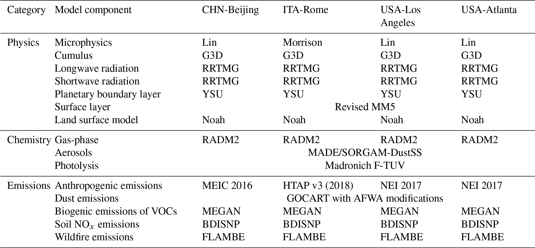
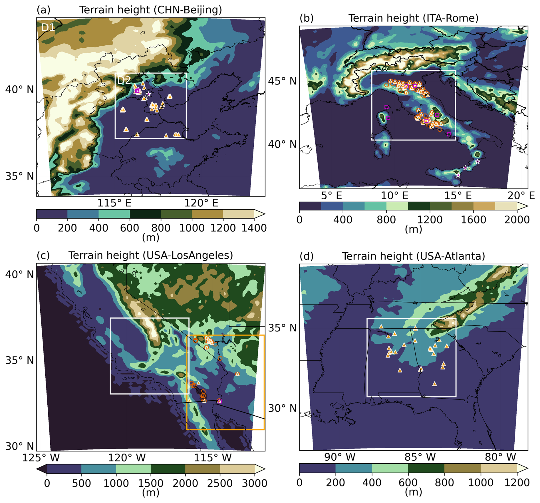
Figure 2 Terrain height for (a) CHN-Beijing, (b) ITA-Rome, (c) USA-LosAngeles and (d) USA-Atlanta target areas of the 2 nested domains: the outer domain (D1) and the inner domain (D2) shown as the white box. For (a), the orange filled triangles represent the ground observation sites of PM_2.5 and PM₁₀ mass concentration. Both open magenta squares and stars represent the AERONET ground observation sites. The sites denoted by the stars are used to constrain the dust particle size distribution as described in Sect. 4.1, while the sites denoted by squares are used to evaluate model simulated AOD. (b) is same as (a), except that the orange open circles represent ground observations of PM₁₀ mass concentration, and orange filled triangles are the ground observations sites of PM_2.5 mass concentration. (c) is the same as (b) except that the orange box is defined as the dust-prone region, which is used to tune dust emissions. For (d), orange filled triangles represent the ground observation sites of PM_2.5 mass concentration.

There are many physics schemes that can be used in WRF-Chem. We select the commonly used schemes for each target area based on literature review and our previous work (e.g., Yang et al., 2013; Sha et al., 2021; Zhang et al., 2022). We also consider a few other factors as described below. For the cumulus scheme, we consider the Grell 3D ensemble (G3D, Grell and Dévényi, 2002) scheme, which also accounts for cloud radiation feedback. For model spatial grids greater than 10 km, they usually rely on the cumulus parameterization to determine the subgrid convective processes. For model spatial grids smaller than 10 km, it is generally considered as the convective gray zone, where the use of convective parameterization or explicit resolving treatment of the convective process remains to be an ongoing question (Jeworrek et al., 2019). Typically, for model spatial grids larger than 5 km, convective parameterization has been used in regional model studies (e.g., Zhang and McFarlane, 1995; Clark et al., 2009; Dudhia, 2014). For model spatial grids smaller than 5 km, generally considered convection-permitting scale, numerous regional model studies have suggested to turn off the cumulus scheme (e.g., Prein et al., 2015; Wang et al., 2021b; Weisman et al., 1997; Weisman et al., 2008; Done et al., 2004; Gao et al., 2017), especially if the cumulus scheme is not scale-aware (Wagner et al., 2018). Therefore, we have chosen to turn off the cumulus scheme here for the inner domain (D2) with the 4 km spatial resolution.

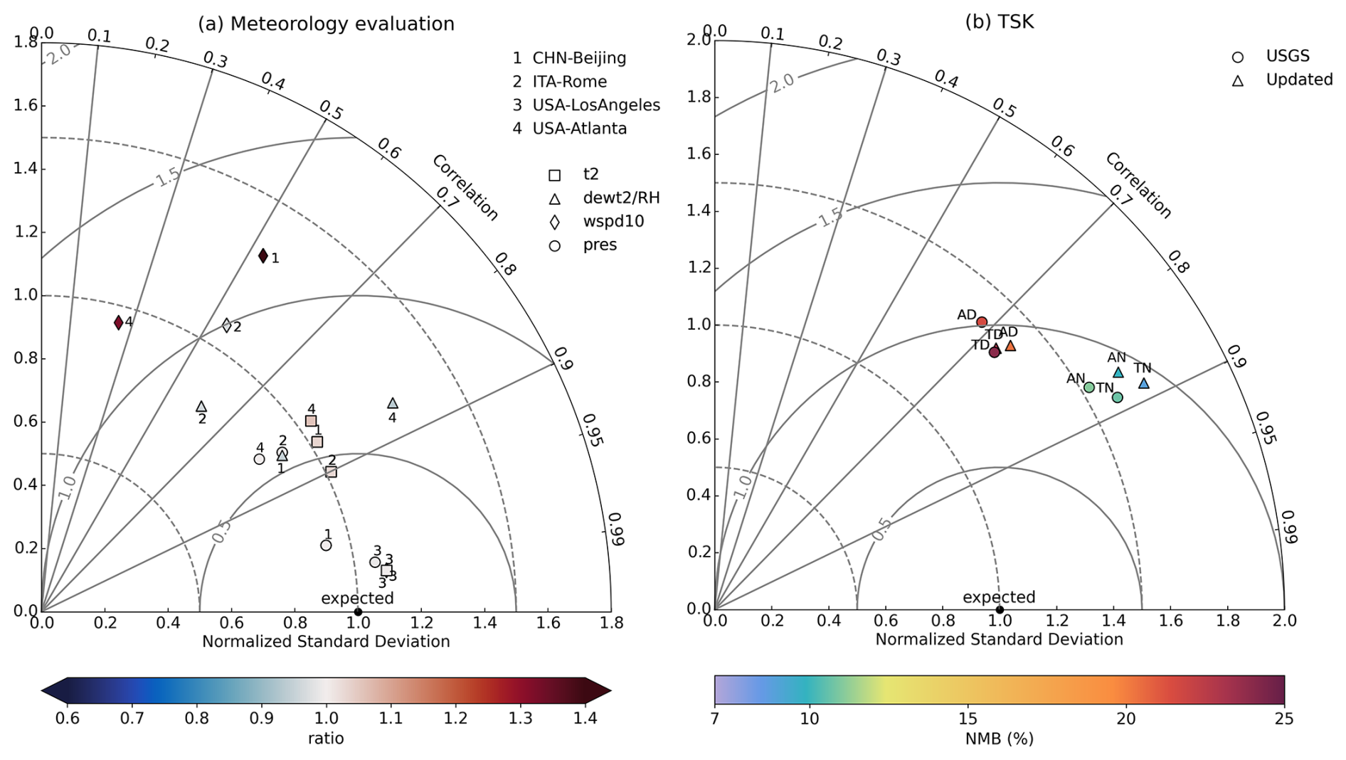
Figure 3 Taylor Diagrams for evaluating UI-WRF-Chem model simulated (a) meteorological variables (t2, dewt2 or RH, wspd10 and pres) with ground observations for CHN-Beijing, ITA-Rome, USA-LosAngeles and USA-Atlanta target areas, and (b) surface skin temperature (TSK) with MODIS observed land surface temperature (LST) for CHN-Beijing during July 2018. In (a), evaluation results of daily meteorology variables are based on the model final configuration for each target area (Table 1). Color bar represents the ratio between model results and ground observations. In (b), USGS and updated refer to the UI-WRF-Chem sensitivity simulations 2N_def (default USGS land cover type and subsequently derived GVF, LAI and albedo) and 2N_upd (updated land cover type, GVF, LAI and albedo with MODIS land data) in Table 2, respectively. UI-WRF-Chem simulated TSK averaged over the Terra and Aqua overpass time during daytime (TD and AD) and nighttime (TN and AN), respectively are compared to the corresponding Terra and Aqua observations. Color bar represents the normalized mean bias (NMB) between model results and satellite observations.

With the current version (WRF-Chem v3.8.1) of the code, chemical species are transported using the G3D scheme, regardless of which cumulus scheme is used, while other scalars are transported with the selected cumulus scheme. Therefore, the G3D scheme is used to ensure the consistency between chemistry and physics. Additionally, WRF-Chem v3.8.1 was selected as the base version at the beginning of this project due to its stability. We have maintained this version over the course of the project to ensure the consistency and reproducibility of the results. Although there are several scale-aware cumulus schemes available in WRF-Chem such as the Kain-Fritsch scheme (KF, Kain, 2004) and the Grell-Freitas scheme (GF, Grell and Freitas, 2014), only the GF scheme has been updated to ensure the consistent transport of both chemical species and other scalars, as described by Li et al. (2018, 2019). We acknowledge the limitation of using only the G3D scheme in this work and plan to update the UI-WRF-Chem modeling framework to a newer version to enable the use of the GF scheme and incorporate other recent improvements as well.

For the microphysics scheme, an inexpensive scheme is typically sufficient for model spatial grids greater than 10 km but a more complex scheme that accounts for the prediction of the mixed phases (6-class schemes, including graupel) and number concentrations (double-moment schemes) is required (Han et al., 2019). Therefore, we consider these three schemes in the current work: the Lin scheme (Lin et al., 1983; Chen and Sun, 2002), the WRF Single-Moment 6-Class Microphysics Scheme (WSM6) (Hong and Lim, 2006) and the Morrison scheme (Morrison et al., 2009). The former two is a single-moment 6 class scheme and the latter one is a double-moment scheme, which also predicts the number concentration of the hydrometer besides the total amount. All the three schemes include the simulations of graupel which is shown to help with the simulation of convection for higher resolution simulation (Brisson et al., 2015). At convective-permitting scales, the graupel size representation could play a more important role in the precipitation prediction than the number of moments (single vs. double) in certain cases (Adams-Selin et al., 2013).

For the shortwave radiation scheme, we only consider the two-stream multiband Goddard scheme (Chou et al., 1998) and the Rapid Radiative Transfer Model for GCMs (RRTMG) (Iacono et al., 2008), which both include the direct aerosol radiation feedback. For the longwave radiation, we select the RRTMG and the Rapid Radiative Transfer Model (RRTM) schemes (Mlawer et al., 1997). RRTMG for both shortwave and longwave radiation schemes are recommended to pair together in the model by the developing team of WRF-Chem. For the planetary boundary layer (PBL) scheme and the corresponding surface layer scheme, we consider the nonlocal boundary layer scheme – the Yonsei University scheme (YSU, (Hong et al., 2006)) with the revised fifth-generation Pennsylvania State University – National Center for Atmospheric Research Mesoscale Model (MM5) (Grell et al., 1994; Jiménez et al., 2012) surface layer scheme. We also consider two commonly used local boundary layer schemes: Mellor-Yamada-Janjic (MYJ, (Janjic, 2001)) with the ETA similarity surface layer scheme; Mellor-Yamada-Nakanishi-Niino level 2.5 (MYNN2.5, (Nakanishi and Niino, 2004)) with the MYNN surface layer scheme. When using the YSU scheme, we also turn on the surface drag parameterization (Jiménez and Dudhia, 2012) to improve topographic effects on surface winds over a complex terrain. The land surface model is the Noah land model (Chen and Dudhia, 2001), which incorporates our updates of the land surface properties as described in Sect. 2.4. Additionally, for a specific target area, other physics schemes not mentioned here but commonly used in that area will also be tested.

Details regarding the selection and evaluation results of the physics scheme for the four target areas are available in Sect. S2. Here, we provide a summary of the evaluation results. Sensitivity simulations performed for each target area are listed in Table S1 and we focus on testing the following schemes: microphysics, shortwave and longwave radiation and PBL. We evaluate four UI-WRF-Chem simulated meteorology variables with surface observations: air temperature at 2 m (t2), dew temperature at 2 m (dewt2) or relative humidity (RH), wind speed at 10 m (wspd10) and sea level pressure (pres). Results of the hourly or 3-hourly evaluation of the meteorology variables are summarized in Table S2 and Fig. S1. Overall, all the sensitivity simulations of t2 and pres for all the target areas show the highest correlation (> 0.8). Dewt2 or RH also show good correlation (0.59–0.84) with ITA-Rome showing the lowest correlation. The case study of ITA-Rome is conducted over June 2023, where some regions in Italy experienced rainfall events about one third of the month. Uncertainties of UI-WRF-Chem capturing the rainfall events (discussed in Sect. 4.2) could result in the lower correlation of RH. Comparatively, wspd10 shows lower correlation (0.22–0.52) over USA-Atlanta. Across the target areas, we find that wspd10 is most sensitive to the PBL scheme compared with other schemes tested, which is also found in previous studies (e.g., Yu et al., 2022). It is found that no single combination of the physics scheme will result in the best performance for each meteorology variable evaluated. The interaction of these different parameterized processes mentioned above (e.g., convection, boundary layer mixing, microphysics and radiation) are complex (Prein et al., 2015) and it is region, case and variable specific. Therefore, model performance can vary from region to region or case to case.

Based on the evaluation results, we select the optimal combination of various physics schemes tested as the final configuration for each target area (Tables S1 and 1). We summarize the statistics of the evaluation of the daily meteorology variables for the four target areas in Fig. 3a, for the final configuration only. We find that UI-WRF-Chem simulated daily t2, dewt2 and pres all show high correlation (> 0.7) and low NMB (−10 % to +10 %) across the target areas. For evaluation of daily wspd10, correlation increases, and bias decreases compared with hourly evaluation. For USA-Atlanta, the daily wspd10 still shows lower correlation (∼ 0.25) compared with other target areas. The sensitivity simulation over USA-Atlanta is conducted over June 2022 and majority of the wspd10 are under 5 m s⁻¹. It can be challenging for the model to capture this stable condition very well. Future work could focus on trying nudging with ground observation to improve the model performance over this area. We also recognize that our sensitivity tests are limited to one month for each target area. We are not able to test the performance for different seasons. Nevertheless, it provides values for understanding the model sensitivity to different schemes at different locations.

Biogenic emissions for VOCs are from the MEGAN scheme and soil NO_x emissions are from the BDISNP scheme. Fire emissions are from the FLAMBE emission inventory and dust emissions use the GOCART with AFWA modification. Here, we use MEIC 2016 as the anthropogenic emission for CHN-Beijing and NEI 2017 emission inventory for USA-LosAngeles and USA-Atlanta. The HTAP_v3 2018 is used for ITA-Rome. The gas-phase chemistry is the RADM2, and the aerosol module is the newly added scheme MADE/SORGAM-DustSS: the MADE/SORGAM scheme with the addition of dust and sea salt aerosol species as described in Sect. 2.7. Lastly, we use the Madronich Fast Tropospheric UV and Visible Radiation Model (F-TUV) as the photolysis scheme (Madronich, 1987; Tie et al., 2003).

4 Case studies for different target areas

4.1 Case study – CHN-Beijing

Beijing and its surrounding area in China, are affected by both local and regional emissions as well as long-range transport (Wu et al., 2021; Zhang et al., 2018). In recent decades, the North China Plain including the Beijing area has experienced severe PM pollution problems as a result of the rapid economic growth and urbanization (Zhang et al., 2016). In addition to the impacts of anthropogenic emission on surface PM levels, strong dust storms from the Taklamakan Desert and the Gobi Desert sometimes can be transported downwind to the Beijing area and affect local air quality in the springtime. Here for the CHN-Beijing target area (Fig. 2a), we first focus on a dust intrusion event during 24–31 March 2018, to study the impacts of chemical boundary conditions on surface PM. Figure 4 shows the MODIS Aqua observed AOD over part of China for the period of this event. The dust storm can be seen on 26 March 2018, at both Taklamakan and Gobi Deserts and by 28 March, strong dust clouds have been transported to Beijing and its surrounding areas. Figure S2 displays the movement of surface observations of daily PM₁₀ mass concentration across China from 24 March to 31 March 2018. On 27 and 28 March 2018, high surface PM₁₀ concentration were observed in Beijing, Tianjin and Hebei province with hourly concentration exceeding 1000 µg m⁻³ (not shown here). Then, we focus on July 2018 to study the impacts of updating land surface properties and soil NO_x emission scheme on model performances.

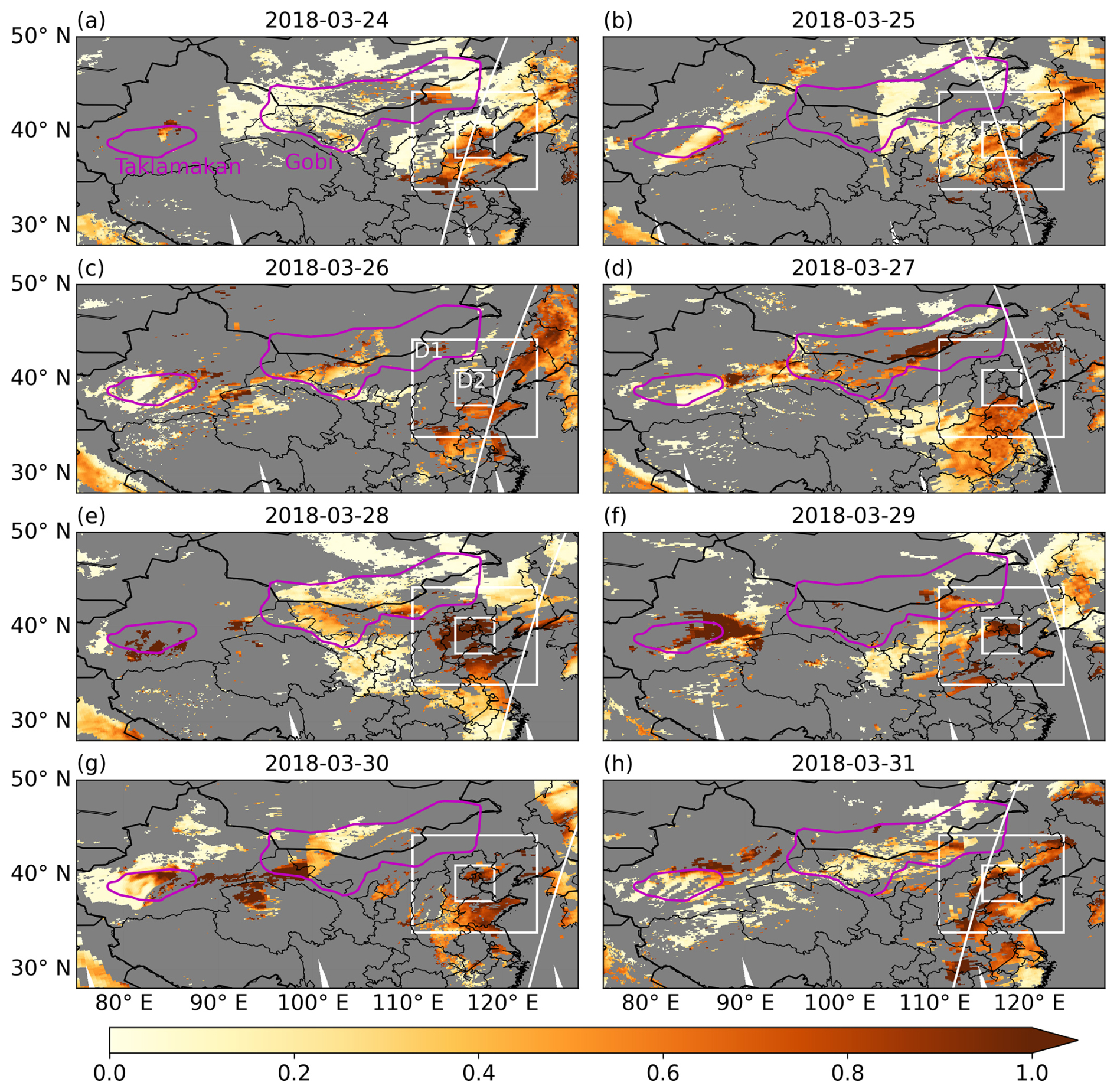
Figure 4 (a–h) MODIS Aqua Deep Blue (DB) AOD from 24–31 March 2018. The white boxes represent the UI-WRF-Chem 2 nested domains for outer (D1) and inner domain (D2) over CHN-Beijing, respectively. The white diagonal lines indicate the CALIOP tracks. The magenta contour lines represent the boundaries of Taklamakan and Gobi Deserts.

4.1.1 Sensitivity experiment design

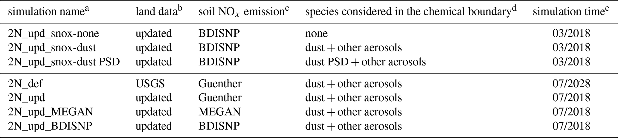
For CHN-Beijing target area, we carry out a suite of sensitivity simulations using the UI-WRF-Chem framework as shown in Table 2 to investigate the impacts of chemical boundary conditions, updated land surface properties and soil NO_x emission scheme on model performance. First, three simulations are conducted during March 2018 to study the impacts of using MERRA-2 data to provide chemical boundary conditions on model performance. Additionally, four simulations are carried out for July 2018 to investigate the impacts of updating land surface properties as well as surface soil NO_x emission scheme. The simulation with “2N_def” uses the default USGS land cover type and subsequently derived GVF, LAI and albedo, using a predefined look-up table. The simulations with “2N_upd” uses the corresponding updated land cover type, GVF, LAI and albedo, based on the MODIS land data products for the simulation period, as described in Sect. 2.4. The simulations with “2N_*_snox*” use our newly developed BDISNP soil NO_x emission scheme.

Table 2 A suite of UI-WRF-Chem sensitivity simulations with different chemical boundary conditions, land data and soil NO_x emission schemes for CHN-Beijing.

^a The simulation name starting with “2N*” refers to the 2 nested domains used for CHN-Beijing as shown in Fig. 2a. The 2 nested domains have a horizontal spatial resolution of 4 km × 4 km and 12 km × 12 km for the inner and outer domain, respectively.
^b We test different land surface properties used for the UI-WRF-Chem static input data. The simulation name with “^*def^*” refers to the use of USGS land cover type data and subsequently derived GVF, LAI and albedo, with a predefined look-up table. The simulation name with “^*upd^*” refers to the use of updated land cover type, GVF, LAI and albedo data with MODIS land data products.
^c We test different soil NO_x emission schemes. The Guenther scheme calculates biogenic emissions including soil NO_x emissions, without any external input datasets needed. The MEGAN scheme requires external input files to calculate biogenic emissions including soil NO_x emissions. The BDISNP is our newly developed scheme. Since the USGS land data is only compatible with the Guenther scheme, we conduct sensitivity simulations “2N_def” and “2N_upd” to evaluate the impacts of updating land surface properties. The simulation name with “^*snox^*” means that the BDISNP soil NO_x emission scheme is used.
^d We test different scenarios of chemical species used in MERRA-2 data for updating UI-WRF-Chem chemical boundary conditions. “None” (simulation name with “*none*”) means that chemical boundary conditions from MERRA-2 data are not used but instead the model default chemical boundary conditions are used. They represent a clean North American summer day, which includes a limited number of chemical species and most of them are gas species. For aerosol species, the concentrations are close to zero values. “dust + other aerosols” (simulation name with “*dust*”) means that dust and other aerosols including sulfate, BC and OC are considered in the chemical boundary conditions from MERRA-2 data. “dust particle size distribution (PSD) + other aerosols” (simulation name with “^*dust PSD^*”) is the same as “dust + other aerosols” except that we use the ratio of averaged PSD from AERONET observations and MERRA-2 data over 2000–2020 to scale the dust concentration for each size bin in the MERRA-2 data. More details can be found in Sect. 4.1.1.
^e We conduct the sensitivity simulations in two different time periods: March and July 2018, respectively. The simulations in March focus on evaluating the impacts of using MERRA-2 data to provide chemical boundary conditions on model performance while the simulations in July focus on the impacts of updating land surface properties with MODIS data and soil NO_x emission scheme.

The impacts of chemical boundary conditions are evaluated from several sensitivity experiments. In the simulation “2N_upd_ snox-none”, no chemical species from MERRA-2 data are transported into the domain. In the simulation “2N_upd_ snox-dust”, dust and other aerosols including sulfate, BC and OC are considered in the chemical boundary condition from MERRA-2 data. Furthermore, to constrain the chemical boundary condition for the allocation of dust concentration as a function of different size bins, we analyze the AERONET measured aerosol volume size distribution (AVSD) data from 2000 to 2020. If the fine mode fraction (FMF) of AOD at 500 nm is less than 0.3 (Lee et al., 2017), it is considered as a dust event. Figure 5a shows the averaged dust particle size distribution (PSD) over the AERONET sites (Fig. 2a) between 2000–2020 from both AERONET and MERRA-2 data for all the dust events that occurred in CHN-Beijing. The ratio between the mean of the AERONET PSD and MERRA-2 PSD for each of the five dust size bins is then used as a constraint to scale the dust concentration in each bin in the MERRA-2 chemical boundary data. The sensitivity run “2N_upd_snox-dust PSD” in Table 2 is based on this result.

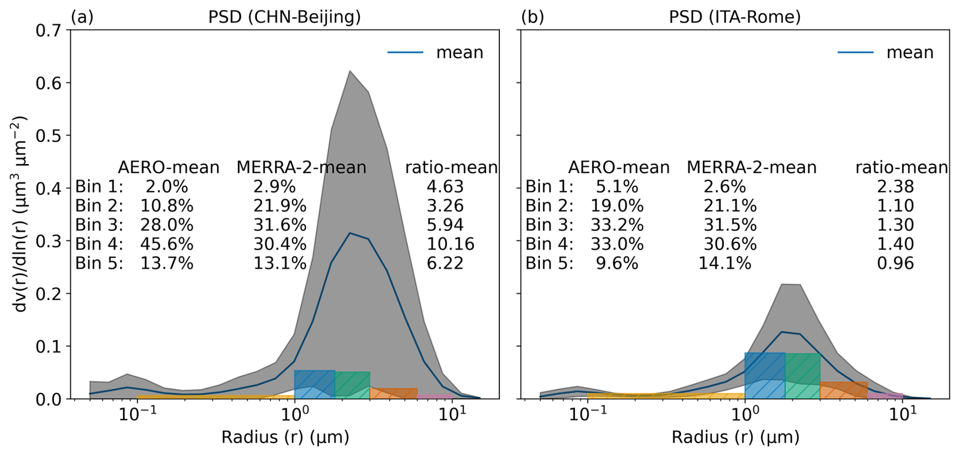
Figure 5 Averaged particle size distribution (PSD) from AERONET observations (blue line) and MERRA-2 data (the 5 colored bins) for (a) CHN-Beijing and (b) ITA_Rome over 2000–2020 and 2000–2023, respectively. The AERONET sites used are shown as stars in Fig. 2a and b, respectively. The dark gray areas represent the AERONET variability. AERO-mean and MERRA-2 mean represent the fraction of the PSD from each bin over the sum of the 5 bins. Ratio-mean is the ratio of the total PSD of AERONET over MERRA-2 for each bin.

Three UI-WRF-Chem sensitivity simulations in Table 2 are run from 18 to 31 March 2018, for evaluating the impacts of using MERRA-2 data to provide chemical boundary conditions. The simulation results with the first 6 d are used as initialization. Model output from 24 to 31 March 2018, are used for analysis, unless noted otherwise. The rest of the four simulations are used for evaluating the impacts of updating land surface properties and soil NO_x emission scheme on model performance. They are carried out from 24 June to 31 July 2018, and model outputs from 1 to 31 July are used for data analysis. We mainly use model output from the inner domain (D2) for data analysis unless noted otherwise.

4.1.2 Impacts of chemical boundary conditions on surface PM and AOD

First, we evaluate the effectiveness of using MERRA-2 data to provide chemical boundary conditions in capturing this dust long-range transport event in spring 2018. Figure 6 shows the overall evaluation of model simulated hourly surface PM_2.5 mass concentration against ground observations over PTA-Beijing during 24–31 March 2018. Results are presented for three sensitivity experiments, as described in Sect. 4.1.1. WRF-Chem PM data are regridded onto the MERRA-2 grid to ensure a fair comparison. Without considering any chemical species in the boundary, the UI-WRF-Chem simulated PM_2.5 concentration (2N_upd_snox-none) substantially underestimates ground observations with a MB of −66.4 µg m⁻³. After including dust and other aerosols in the boundary conditions, the UI-WRF-Chem simulated PM_2.5 concentration (2N_upd_snox-dust) increases from 18.7 to 35.5 µg m⁻³ and thus reduces the MB to −49.6 µg m⁻³. The correlation (R) increases from 0.19 to 0.51 and MAE decreases from 66.7 to 50.2 µg m⁻³ (paired t-test, adjusted p<0.05; Bonferroni correction). By constraining the dust PSD in the MERRA-2 data with the AERONET climatology data, the UI-WRF-Chem simulated PM_2.5 (2N_upd_snox-dust PSD) further improves the model performance with MB of −24 µg m⁻³, R of 0.54 and MAE of 37.0 µg m⁻³ (paired t-test, adjusted p < 0.05; Bonferroni correction). This sensitivity simulation also outperforms the MERRA-2 simulated surface PM_2.5 concentration with MB of −33.7 µg m⁻³, R of 0.39 and MAE of 41.7 µg m⁻³ (paired t-test, adjusted p < 0.05; Bonferroni correction).

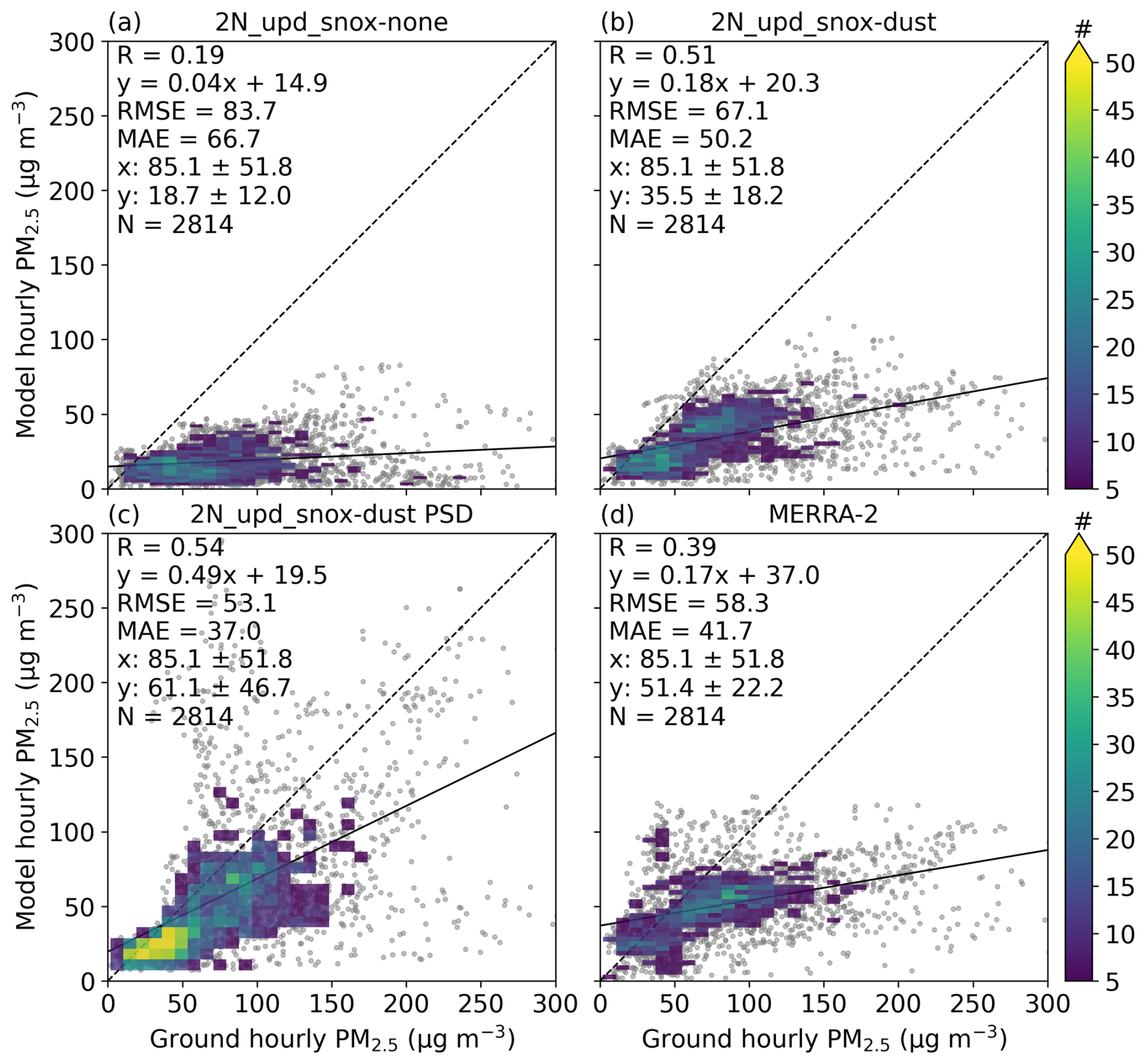
Figure 6 Scatter plot of hourly surface PM_2.5 concentration between model (y axis) and ground observation (x axis) for surface sites in the inner domain (D2) of CHN-Beijing for 24–31 March 2018. (a)–(c) refer to the UI-WRF-Chem sensitivity simulations with different chemical boundary conditions being considered using MERRA-2 data (Table 2). (a) no chemical species, (b) dust and other aerosols and (c) same as (b) except that the dust concentration is scaled based on constraining MERRA-2 dust PSD data with AERONET PSD climatology data. (d) is from MERRA-2 simulated surface PM_2.5 concentration. Also shown on the scatter plot is the correlation coefficient (R), the root-mean-square error (RMSE), the mean absolute error (MAE), the mean ± standard deviation for observed (x) and model-simulated surface PM_2.5 (y), the number of collocated data points (N), the density of points (the color bar), the best fit linear regression line (the solid black line) and the 1:1 line (the dashed black line). WRF-Chem PM data are regridded onto the MERRA-2 grid, and when multiple surface sites fall within the same MERRA-2 grid, the observations are then averaged to represent a single collocated site.

Figures 7a and S3 show the time series of hourly surface PM_2.5 and PM₁₀ concentration from 24–31 March 2018 for both model simulations and ground observations. During 27–28 March, when the dust front intruded PTA-Beijing, hourly observations of surface PM_2.5 and PM₁₀ concentration averaged over all the sites could reach approximately 150 and 900 µg m⁻³, respectively. The UI-WRF-Chem simulation without chemical boundary conditions (2N_upd_ snox-none) misses this peak for both PM_2.5 and PM₁₀ while both the UI-WRF-Chem simulation with chemical boundary condition (2N_upd_snox-dust) and MERRA-2 data capture this peak for PM_2.5 but miss the peak for PM₁₀. The UI-WRF-Chem simulation with dust PSD constrained (2N_upd_snox-dust PSD) capture the peaks of both PM_2.5 and PM₁₀. Compared with the simulation without boundary conditions (2N_ upd_snox-none), adding chemical boundary conditions (2N_upd_snox-dust) improves model performance with increased correlation for both PM_2.5 (0.41 to 0.72) and PM₁₀ (0.06 to 0.23). The simulation with dust PSD constrained (2N_upd_snox-dust PSD) does not improve the correlation of PM_2.5 (0.65) but does for PM₁₀ (0.28), compared with the simulation using dust in the chemical boundary (2N_upd_snox-dust). Time series of UI-WRF-Chem simulated hourly speciated PM_2.5 (e.g., OC, EC, sulfate, nitrate) and dust components in both PM_2.5 and PM₁₀ from the two sensitivity simulations (2N_upd_snox-dust and 2N_ upd_snox-dust PSD) (not shown here) indicate that only the dust components exhibit similar peaks as in the total PM_2.5 and PM₁₀, while other speciated PM_2.5 components do not follow the same temporal pattern. This demonstrates that the observed peaks in both PM_2.5 and PM₁₀ are primarily driven by the dust intrusion event. Moreover, the magnitude of the peak from the sensitivity simulation – 2N_upd_snox-dust PSD is larger and matches better with surface observations, especially for PM₁₀, than that of the 2N_upd_snox-dust. This further highlights the effectiveness of our method in improving the representation of dust size distribution in MERRA-2 data.

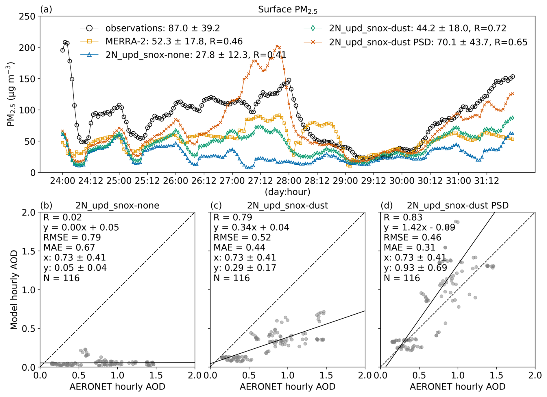
Figure 7 (a) time series of hourly surface PM_2.5 concentration averaged over surface sites in the inner domain (D2) of CHN-Beijing for 24–31 March 2018, from model simulations and ground observations. 2N_upd_snox-none/dust/dust PSD refer to the UI-WRF-Chem sensitivity simulations with different chemical boundary conditions being considered using MERRA-2 data (Table 2): no chemical species; dust and other aerosols; dust concentration is scaled based on constraining MERRA-2 dust PSD data with AERONET PSD climatology data. Also shown on the plot is the mean ± standard deviation of surface PM_2.5 for model simulations or observations as well as the correlation coefficient (R). (b–d): scatter plot of hourly AOD between model (y axis) and AERONET observation (x axis) for 24–31 March 2018. Also shown on the scatter plot is R, the root-mean-square error (RMSE), the mean absolute error (MAE), the mean ± standard deviation for observed (x) and model-simulated AOD (y), the number of collocated data points (N), the best fit linear regression line (the solid black line) and the 1:1 line (the dashed black line).

Not only does considering chemical boundary conditions improve surface PM mass concentration, it also enhances the total aerosol column amount and vertical distribution. Figure 7b–d shows the AOD evaluation between model simulations and AERONET observations. Without considering boundary conditions, the UI-WRF-Chem simulation (2N_upd_snox-none) significantly underestimates the AERONET observed AOD (0.05 vs. 0.73) and shows poor correlation (0.02). Including dust and other aerosols (2N_upd_snox-dust) increases UI-WRF-Chem simulated AOD (0.29), improves correlation (0.79) and reduces MAE from 0.67 to 0.44 (paired t-test, adjusted p > 0.05; Wilcoxon, adjusted p < 0.05; Bonferroni correction). Further constraining the dust in the boundary (2N_upd_snox-dust PSD) yields the best model performance with simulated AOD of 0.93 and correlation of 0.83, reducing MAE from 0.44 to 0.31 (paired t-test, adjusted p > 0.05; Wilcoxon, adjusted p < 0.05; Bonferroni correction). The paired t-test does not find statistically significant changes in the MAE, likely due to the smaller sample size, whereas the Wilcoxon test shows that changes in the MAE are statistically significant.

We then compare the UI-WRF-Chem simulated vertical aerosol profile with the Cloud-Aerosol Lidar with Orthogonal Polarization (CALIOP) data for the outer domain (D1) during 26–28 March, when dust reaches the PTA-Beijing domain. Figure 8 shows the CALIOP derived aerosol extinction coefficient, aerosol type as well as UI-WRF-Chem simulated extinction coefficient. The CALIOP ground tracks are located within the UI-WRF-Chem outer domain (D1) (Fig. 4) and model grids that overlap with the tracks are selected. From both CALIOP aerosol extinction coefficient and aerosol type, we can see that dust is dominating the vertical distribution above ∼ 3–4 km and mixed with marine and anthropogenic aerosols in the boundary layer. Without considering aerosols in the chemical boundary conditions, the UI-WRF-Chem simulated extinction coefficient is negligible above the boundary layer (not shown here). After considering dust and other aerosols in the chemical boundary, we can see the increase in the extinction coefficient in the vertical distribution (Fig. 8g–i). Constraining the dust PSD in the boundary (2N_upd_snox-dust PSD, Fig. 8j–l) further enhances the vertical distribution of the aerosol extinction coefficient, which matches better with the CALIOP observations. This reflects the effectiveness of including dust and other aerosols in the chemical boundary condition to better capture the vertical distribution of aerosol properties in this dust intrusion event. We note that CALIOP data is also subject to uncertainties of the lidar ratio used in deriving the extinction, and so is the extinction modeled by UI-WRF-Chem (Yang et al., 2013). Hence, CALIOP data is used as a relative reference to assess the model improvement.

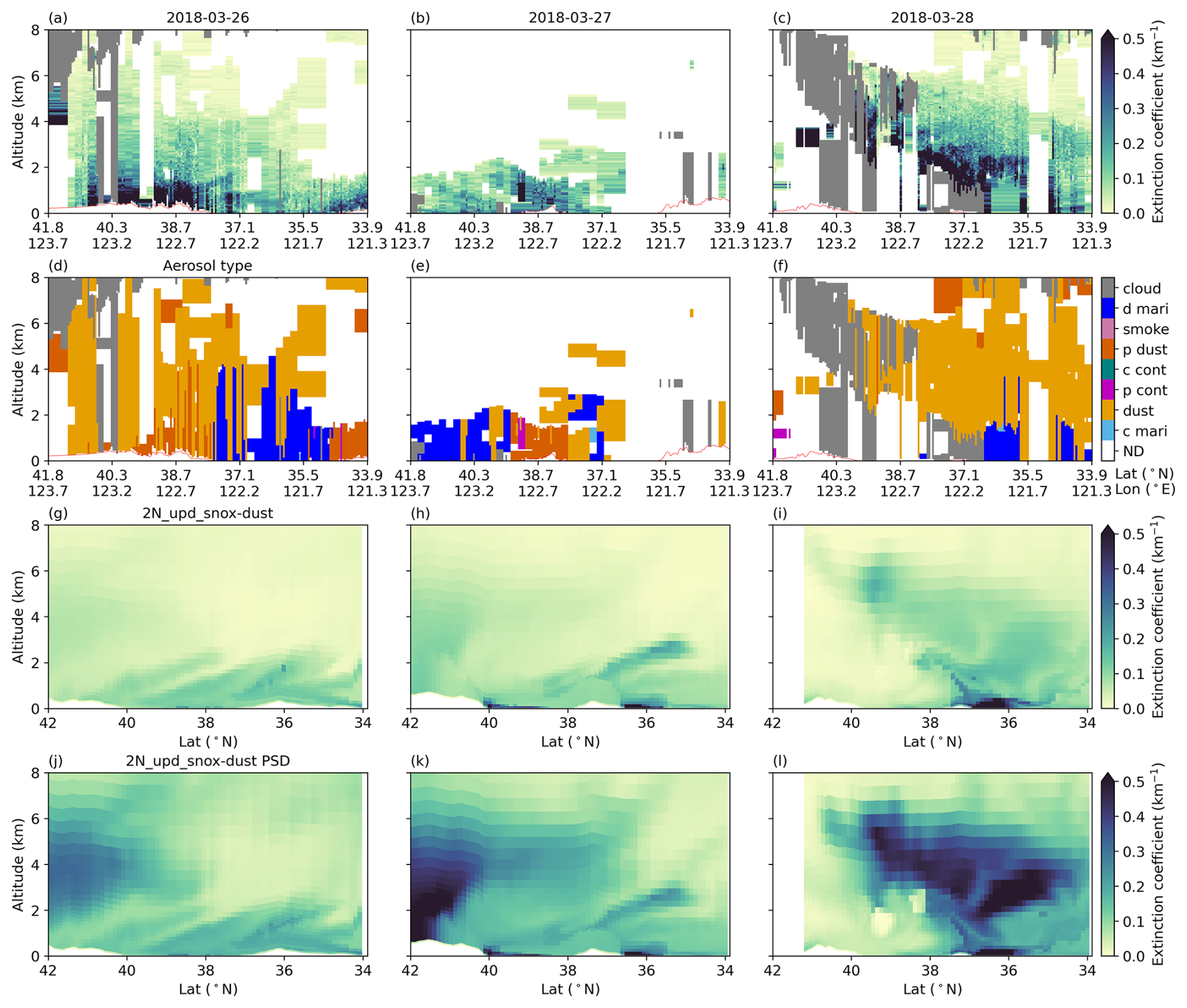
Figure 8 Comparison of CALIOP–derived vertical profile of aerosol extinction coefficient (532 nm, a–c) and aerosol type (d–f) with UI-WRF-Chem simulated extinction coefficient for CHN-Beijing over 26–28 March 2018. UI-WRF-Chem outputs are from the outer domain (D1) that overlap with CALIOP tracks (Fig. 4). (g)–(i) are the extinction coefficients from the UI-WRF-Chem sensitivity simulation 2N_upd_snox-dust, where dust and other aerosols are considered in the MERRA-2 chemical boundary conditions. (j)–(l) are the extinction coefficients from UI-WRF-Chem sensitivity simulation 2N_upd_snox-dust PSD where dust concentration is scaled in the MERRA-2 chemical boundary conditions, based on constraining MERRA-2 dust PSD data with AERONET PSD climatology data. In (a)–(f), the gray areas represent cloud. In (d)–(f), different aerosol types are classified: d mari for dusty marine, p dust for polluted dust, c cont for clean continental, p cont for polluted continental and c mari for clean marine. ND includes areas that have clean air and aerosol type not being determined.

Since PTA-Being is located downwind of the dust source regions in this case, there could be uncertainties in simulating the transport of different dust size bins in MERRA-2 data from source regions. Thus, our constraining method could provide an effective way to improve the dust size distribution in the boundary conditions and subsequently improve model simulated surface PM concentration as well as vertical distribution of aerosols. This method could also benefit other PTAs such as ITA-Rome, that can be affected by dust transport events, which will be discussed in Sect. 4.2.

4.1.3 Impacts of updated land surface properties on model performance

The UI-WRF-Chem model simulated surface skin temperature (TSK) is evaluated with satellite observations of land surface temperature (LST) from MODIS onboard Terra and Aqua for July 2018. We first regrid the MODIS daily LST data onto the WRF-Chem model grid, and then mask the WRF-Chem output based on the spatial and temporal availability of MODIS data to ensure a fair comparison. The Beijing-Tianjin-Hebei region is one of the highly urbanized clusters in the world and has experienced intense urban heat island (UHI) effects in the past decade (Wang et al., 2016; Clinton and Gong, 2013). First, by comparing the default and updated land cover type (Fig. 9a and f), we can see that the updated land cover type captures the urban growth over the region. The corresponding land surface properties including LAI, GVF and albedo also show changes with the updated data (Fig. S4). Both daytime (∼ 10:30 a.m. and ∼ 01:30 p.m. LT) (Figs. 9b and S5a) and nighttime (∼ 10:30 p.m. and ∼ 01:30 a.m. LT) (Figs. 9g and S5e) LST from MODIS Terra and Aqua show the UHI phenomenon over the region. Our UI-WRF-Chem model simulated TSK with updated land surface properties using MODIS data can capture the UHI spatial pattern with higher temperature in urban areas than rural areas for both daytime and nighttime. It matches the spatial pattern of satellite observed LST UHI better than the UI-WRF-Chem simulation with the use of the default USGS land cover type and other surface properties, which is consistent with our previous work (Wang et al., 2023). Figure 3b shows the Taylor Diagram of comparing UI-WRF-Chem simulated LST with MODIS Terra and Aqua daytime and nighttime, respectively. We find that the UI-WRF-Chem simulated TSK with updated land surface properties decreases the relative bias for both Terra and Aqua daytime and nighttime, compared with the UI-WRF-Chem simulation using the default USGS land surface properties. The model simulated TSK with updated land surface properties also results in an increase in correlation for the Aqua daytime period compared with the model simulation using the USGS land surface properties.

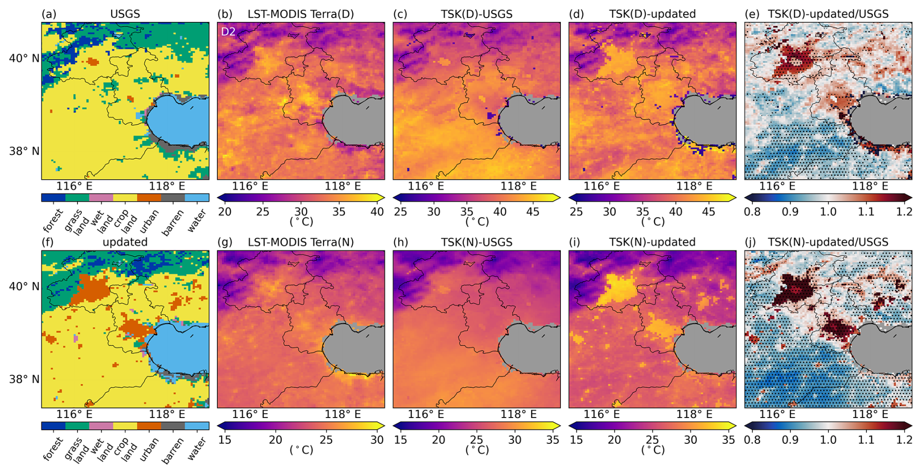
Figure 9 Comparison of UI-WRF-Chem simulated monthly mean surface skin temperature (TSK) with MODIS Terra observed land surface temperature (LST) over the inner domain (D2) of CHN-Beijing for July 2018. (a) and (f) are the land cover type from the default USGS data and updated MODIS land data. (b) and (g) are the MODIS Terra LST during daytime (D) and nighttime (N), respectively. (c) and (d) are model simulated TSK averaged over Terra overpass time during daytime from UI-WRF-Chem sensitivity simulations 2N_def (default USGS land cover type and subsequently derived GVF, LAI and albedo) and 2N_upd (updated land cover type, GVF, LAI and albedo with MODIS land data) in Table 2, respectively. (e) is the ratio between (d) and (c), expressed as the geometric mean of daily ratio, with stippling indicating model grids where the difference is statistically significant (Wilcoxon test, adjusted p<0.05; FDR correction). (h)–(j) are the same as (c)–(e) but averaged over Terra overpass time during nighttime. Oceans are masked as gray colors.

Figure S6 shows the potential impacts of updated land surface properties on model simulated planetary boundary layer height (PBLH) and subsequently on surface PM_2.5 concentration. We find that the PBLH mainly increases in the urban areas where the land surface temperature increases, which in turn leads to a decrease in surface PM_2.5. Our work shows the promising use of updated land surface properties with timely satellite data to better capture the land cover type and other land surface properties for regions with fast urban development. To better study the impacts of UHI in the region, an urban canopy model could be used to include more details about the underlying urban surface feature and better simulate the physical processes in the boundary layer (He et al., 2019; Liang et al., 2021) with a finer spatial resolution, which is beyond the scope of the current work.

4.1.4 Impacts of updated soil NO_x emission scheme on model performance

Our previous work (Sha et al., 2021) has shown the improvement of model simulated NO₂ VCD, when evaluated against TROPOMI NO₂ VCD over croplands in California, using the BDISNP soil NO_x emission scheme. Here, we also use TROPOMI NO₂ VCD to evaluate UI-WRF-Chem simulated NO₂ VCD over croplands in the outer domain (D1) of CHN-Beijing for July 2018. Daily TROPOMI NO₂ data are regridded to UI-WRF-Chem grids with averaging kernels being applied. Hourly data from UI-WRF-Chem output, close to the TROPOMI overpass time (∼ 01:30 p.m. LT) are averaged to compare with TROPOMI data. First, Fig. S7 shows the UI-WRF-Chem simulated monthly mean soil NO_x emissions using the default emission scheme – MEGAN (2N_upd_MEGAN in Table 2) and the updated scheme – BDISNP (2N_upd_BDISNP in Table 2), respectively. The MEGAN scheme (Fig. S7a) simulates low soil NO_x emissions over the whole domain and the BDISNP (Fig. S7b) instead simulates higher soil NO_x emissions in non-urban areas. Croplands show the largest soil NO_x emissions due to the use of fertilizer.

We compare the model simulated tropospheric NO₂ VCD with TROPOMI NO₂ VCD for July 2018 (Figs. 10 and 11). We can find that both simulations underestimate TROPOMI NO₂ VCD (2.2 × 10¹⁵ molec. cm⁻²) by 1.4 × 10¹⁵ and 1.3 × 10¹⁵ molec. cm⁻² for the MEGAN and BDISNP respectively (Fig. 11a and b) over the whole domain. The model simulated NO₂ VCD increases from 1.4 × 10¹⁵ using the MEGAN scheme to 1.7 × 10¹⁵ molec. cm⁻² using the BDISNP scheme over croplands. The BDISNP decreases MAE from 1.59 × 10¹⁵ to 1.53 × 10¹⁵ molec. cm⁻² (paired t-test, adjusted p < 0.05; Bonferroni correction) over the whole domain mainly due to the improvement over croplands. Over croplands, we can see the enhancement in the model simulated NO₂ VCD (Fig. 10c). MAE for croplands decreases from 1.88 × 10¹⁵ molec. cm⁻² to 1.77 × 10¹⁵ (paired t-test, adjusted p<0.05; Bonferroni correction). Both reductions in MAE are statistically significant, underscoring that the improvements are robust, though moderate in magnitude. The increase in soil NO_x emissions has potential impacts on surface nitrate. Figure S8 shows that the increase in surface soil NO_x emissions leads to the increase in surface nitrate up to 30 % in rural areas. Due to the lack of surface observation of nitrate, we are limited to quantify the impacts of the improvement of soil NO_x emissions on surface nitrate. The MAIA satellite mission coupled with the Geostationary Environment Monitoring Spectrometer (GEMS) (Kim et al., 2020) satellite mission could provide a synergetic opportunity to evaluate both gas and aerosol chemistry.

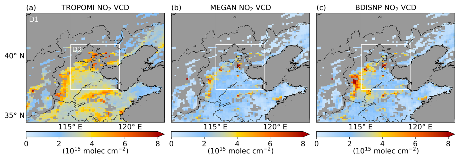
Figure 10 Monthly mean tropospheric NO₂ vertical column density (VCD) over the outer domain (D1) of CHN-Beijing for July 2018 from TROPOMI observation and model sensitivity simulations. Only model grids identified as croplands are shown on the plots and the rest are marked as gray colors. (a) TROPOMI observations; (b) UI-WRF-Chem sensitivity simulation 2N_upd_MEGAN (Table 2) using the MEGAN scheme to calculate soil NO_x emissions; (c) UI-WRF-Chem sensitivity simulation 2N_upd_BDISNP (Table 2) using the BDISNP scheme to calculate soil NO_x emissions. The white box represents the inner domain (D2).

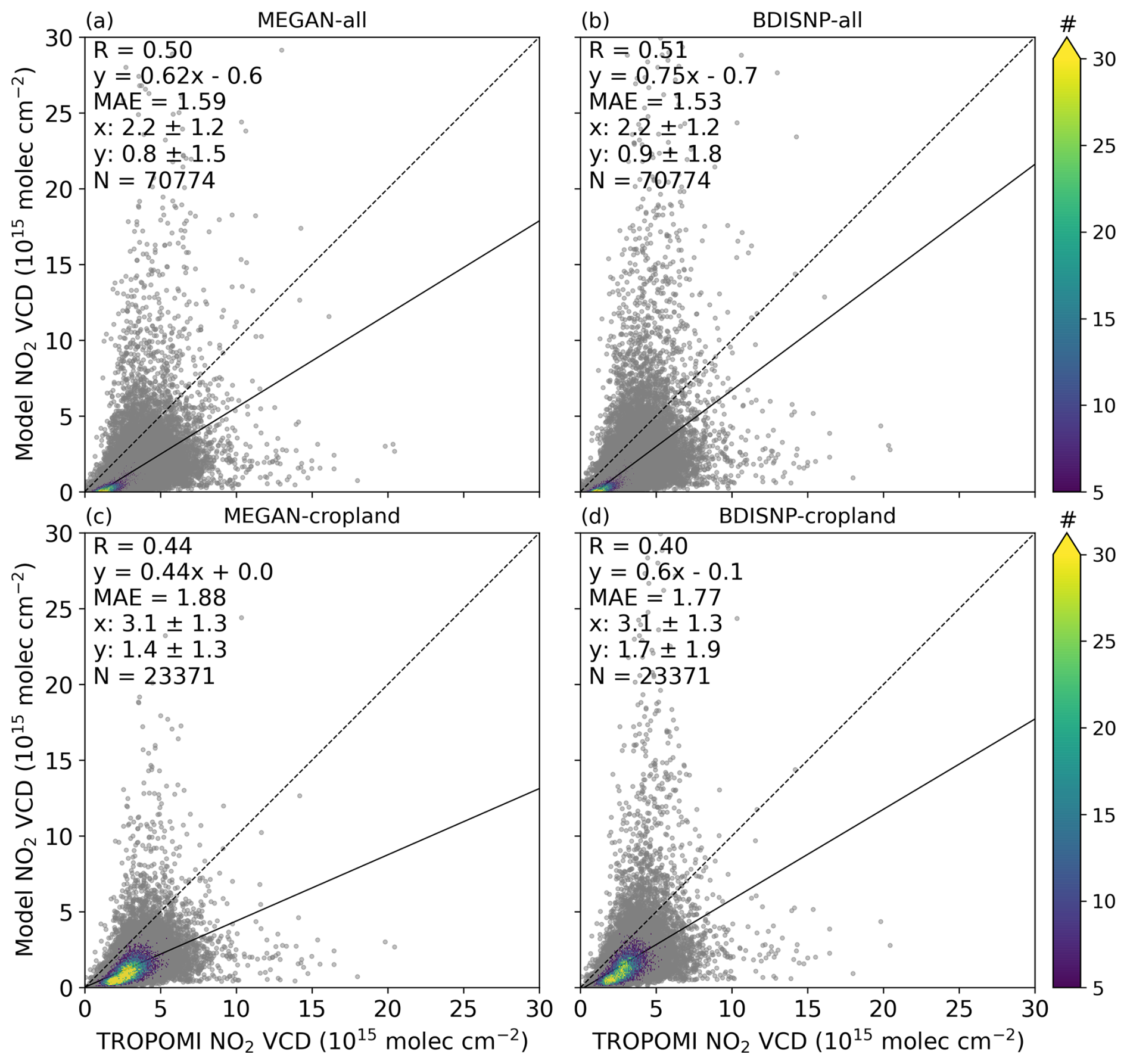
Figure 11 Scatter plot of daily tropospheric NO₂ VCD between model (y axis) and TROPOMI observation (x axis) over the outer domain (D1) of CHN-Beijing for July 2018. (a) and (c) refer to the UI-WRF-Chem sensitivity simulation using the MEGAN scheme (2N_upd_MEGAN in Table 2) and (b) and (d) refer to the sensitivity simulation using the BDISNP scheme (2N_upd_BDISNP in Table 2) to calculate soil NO_x emissions, respectively. (a) and (b) are for model grids over the whole domain while (c) and (d) are for model grids that are identified as croplands. Also shown on the scatter plot is the correlation coefficient (R), the mean absolute error (MAE), the mean ± standard deviation for observed (x) and model simulated tropospheric NO₂ VCD (y), the number of collocated data points (N), the density of points (the color bar), the best fit linear regression line (the solid black line) and the 1:1 line (the dashed black line).

4.2 Case study – ITA-Rome

Our case study over CHN-Beijing target area has demonstrated the benefits of using MERRA-2 data to provide chemical boundary conditions for capturing long-range transport events such as dust intrusion. Some of the other target areas including ITA-Rome are also impacted by dust transport. Saharan dust transport poses a significant concern on air quality in Europe and the Mediterranean Basin. Previous studies have shown that Saharan dust outbreaks are more frequent in southern Europe including Italy than northern Europe (Querol et al., 2009; Viana et al., 2014; Pey et al., 2013; Wang et al., 2020a). For example, Pey et al. (2013) showed that across the Mediterranean Basin, African dust outbreaks occurred from 30 % to 37 % of the annual days in the southern sites and less than 20 % of the days in the northern sites. The work of Barnaba et al. (2022) investigated the impacts of African dust on surface PM₁₀ concentrations in Italy using surface monitoring sites in Italy from 2006–2012 and found that African dust affected surface PM₁₀ levels in Northern and Southern Italy for about 10 % and 30 % of dates in a year, respectively.

Here, we focus on June 2023, where Saharan dust affected PM concentrations in ITA-Rome, and investigate the benefits of using MERRA-2 data to provide chemical boundary conditions for driving UI-WRF-Chem. For example, one Saharan dust intrusion into Italy occurred from 19–22 June 2023 as seen from the VIIRS AOD (Fig. S9) and MERRA-2 simulated dust AOD (not shown here) also captures this dust intrusion event. We conduct three UI-WRF-Chem model sensitivity simulations with different chemical boundary conditions to evaluate model simulated surface PM concentrations and AOD: (1) simulation “2N-none”: no chemical species from MERRA-2 data are transported into the domain; (2) simulation “2N-dust”: dust and other aerosols including sulfate, BC and OC are considered in the MERRA-2 chemical boundary condition; (3) simulation “2N-dust PSD”: dust concentration of different size bins in the MERRA-2 boundary conditions is constrained using the AERONET PSD climatology data from 2000–2023. AERONET sites close to the Saharan dust source region are used for constraining MERRA-2 PSD (Fig. 2b). Figure 5b shows the averaged PSD over the AERONET sites between 2000–2023 from both MERRA-2 and AERONET data. The ratio between the mean of the AERONET PSD and MERRA-2 PSD for each of the five dust size bins is then used as a constraint to scale the dust concentration in each bin in the MERRA-2 chemical boundary data in the simulation “2N-dust PSD”.

Like the case study in CHN-Beijing, using MERRA-2 data to provide chemical boundary conditions for UI-WRF-Chem over ITA-Rome also improves both model simulated surface PM concentration and AOD (Fig. 12). WRF-Chem PM data are regridded onto the MERRA-2 grid for a fair comparison. Compared with the sensitivity simulation 2N-none, the correlation (R) from the sensitivity simulation 2N-dust increases from 0.12 to 0.54, 0.38 to 0.70, and 0.15 to 0.62 for surface PM_2.5, surface PM₁₀ and AOD, respectively, for the whole month of June. The MB decreases from −6.8 to −2.1, −13.8 to −2.3 µg m⁻³, and −0.23 to −0.13 for surface PM_2.5, PM₁₀ and AOD respectively. The MAE decreases significantly from 6.9 to 3.8 µg m⁻³, 13.7 to 9.1 µg m⁻³, and 0.23 to 0.13 (paired t-test, adjusted p<0.05; Bonferroni correction) for surface PM_2.5, PM₁₀ and AOD respectively. Using constrained dust concentration in the MERRA-2 data (2N-dust PSD) further reduces the MB for surface PM_2.5 and AOD and slightly overestimates surface PM₁₀, compared with simulation 2N-dust. In contrast, both MERRA-2 simulated surface PM_2.5 and PM₁₀ overestimate surface observations with MB of 6.4 and 21.8 µg m⁻³, respectively. Both simulations (2N-dust and 2N-dust PSD) show higher correlation than MERRA-2 (0.70 vs. 0.66) when evaluating surface PM₁₀ concentration against ground observations, while simulation 2N-dust PSD shows slightly lower correlation than MERRA-2 for surface PM_2.5 (0.52 vs. 0.54). MAEs from both simulations are also improved significantly (paired t-test, adjusted p<0.05; Bonferroni correction), compared to those of MERRA-2 for both surface PM_2.5 (3.8 vs. 6.7 µg m⁻³; 4.1 vs. 6.7 µg m⁻³) and PM₁₀ (9.1 vs. 22.0 µg m⁻³; 10.3 vs. 22.0 µg m⁻³). Compared with simulation 2N-dust, simulation 2N-dust PSD improves model simulated AOD with MB decreasing from 0.13 to 0.09 and MAE decreases from 0.13 to 0.11 (paired t-test, adjusted p<0.05; Bonferroni correction). MERRA-2 data has the best AOD performance as expected since it assimilates satellite AOD.

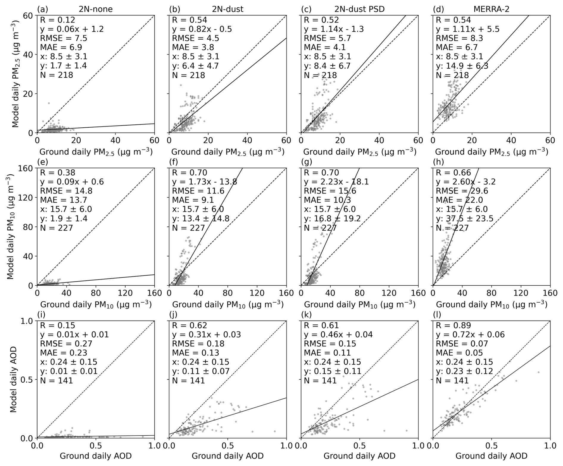
Figure 12 Scatter plot of daily PM_2.5 concentration (a–d), PM₁₀ concentration (e–h), and AOD (i–l), between model (y axis) and ground observation (x axis) over the inner domain (D2) of ITA-Rome for June 2023. (a)–(c), (e)–(g), and (i)–(k) refer to the UI-WRF-Chem sensitivity simulations with different chemical boundary conditions being considered using MERRA-2 data. 2N-none: no chemical species; 2N-dust: dust and other aerosols; 2N-dust PSD: same as 2N-dust except that the dust concentration is scaled based on constraining MERRA-2 dust PSD data with AERONET PSD climatology data. (d), (h) and (l) show the MERRA-2 simulated daily PM_2.5, PM₁₀ and AOD, respectively. Also shown on the scatter plot is the correlation coefficient (R), the root-mean-square error (RMSE), the mean absolute error (MAE), the mean ± standard deviation for observed (x) and model-simulated PM_2.5/PM₁₀/AOD (y), the number of collocated data points (N), the best fit linear regression line (the solid black line) and the 1:1 line (the dashed black line). WRF-Chem PM data are regridded onto the MERRA-2 grid, and when multiple surface PM sites fall within the same MERRA-2 grid, the observations are then averaged to represent a single collocated site.

During June 2023, some parts of the ITA-Rome domain experienced precipitation events (Fig. S10), which occurred mostly during the first half of the month. Compared to the Global Precipitation Measurement (GPM) mission observed precipitation and MERRA-2 simulated precipitation (Fig S10), UI-WRF-Chem simulates higher precipitation, which could result in higher wet deposition of aerosols and lower concentration. Figure S11 shows the comparison of model simulated surface daily PM_2.5 and PM₁₀ with ground observations for the first and second half of the month in June 2023, respectively. We can see that UI-WRF-Chem simulation 2N-dust underestimates both surface PM_2.5 and PM₁₀ during the first half of the month (Fig. S11a–h) with MB of −3.1 and −5.7 µg m⁻³, respectively, while MERRA-2 overestimates surface PM_2.5 and PM₁₀ with MB of 5.1 and 15.7 µg m⁻³, respectively. During the second half of the month (Fig. S11i–p), UI-WRF-Chem simulation 2N-dust underestimates surface PM_2.5 with MB of −1.3 µg m⁻³ but slightly overestimates surface PM₁₀ with MB of 1.3 µg m⁻³. MERRA-2 still overestimates surface PM_2.5 and PM₁₀ with MB of 7.4 and 28.4 µg m⁻³, respectively. Due to the coarse spatial resolution of MERRA-2 data, it may not resolve the localized convective processes well, which could affect the subsequent wet deposition. There are also uncertainties associated with the dust size distribution in MERRA-2 data, which could also affect the wet deposition.

Additionally, uncertainty in UI-WRF-Chem model simulated wet deposition of aerosols could play a role in the model results discussed above. Previous studies have mostly focused on dry dust events (e.g., Zeng et al., 2020), and less has focused on wet dust events, especially dust wet deposition. Jung and Shao (2006) implemented a below-cloud dust wet deposition scheme for the UOC dust emission scheme in WRF-Chem. Currently, no dust wet scavenging scheme is implemented for the original GOCART or GOCART AFWA dust scheme in WRF-Chem. As in previous work (Su and Fung, 2015), we have implemented a simple scheme to allow dust wet scavenging by large scale and convective precipitation by assigning a scavenging efficiency for different dust size bins in the model. Future work will focus on implementing a more complex dust wet deposition scheme to better account for the scavenging processes that consider the dust particle size distribution etc., such as the work of Tsarpalis et al. (2018) and Zhao et al. (2003). Nevertheless, the case study over ITA-Rome again demonstrates the benefits of using MERRA-2 data to drive UI-WRF-Chem for capturing dust transport events.

4.3 Case study – USA-LosAngeles

Each target area has its unique feature of aerosol composition and various factors that affect the aerosol concentration, we have demonstrated the impacts of dust transport on surface PM concentration and AOD over CHN-Beijing and ITA-Rome target areas. Here, we focus on some fine tuning over USA-LosAngeles target area to improve the model simulation of surface PM concentration and AOD.

For the USA-LosAngeles target area (Fig. 2c), we investigate the impacts of dust emissions on surface PM concentration and AOD. Part of the outer domain (D1) over the USA-LosAngeles target area (here defined as the dust-prone region, the orange box in Fig. S12), located in the southwestern U.S., are desert regions with higher soil erodibility than other parts of the domain. It is common in WRF-Chem to tune some of the parameters in the dust emission scheme including the soil erodibility to better match model simulated PM₁₀ concentration and AOD with satellite- and ground-based observations (e.g., Su and Fung, 2015). This approach has been mainly focusing on the total atmospheric dust load instead of an individual dust event and it is sufficient to capture the general magnitude of dust aerosol patterns. We have adopted this simple approach here to do some dust parameter tuning to improve model simulated surface PM₁₀ concentration and AOD with a focus on the overall magnitude.

There are several parameters that can be used to tune dust emissions in the WRF-Chem model. One is the dust_gamma (gamma for short here), which tunes the soil erodibility in an exponential manner. Soil erodibility serves as an important factor for identifying dust source and estimating dust emission flux in the model. The other one is the dust_alpha (alpha for short here), which linearly tunes the total dust emissions. If we use the default setting (gamma = 1, alpha = 1), both model simulated surface daily PM₁₀ concentration and hourly AOD overestimate surface measurements of PM₁₀ and AOD in the dust-prone region (Figs. 13a and j, S13 and S14). Model simulated surface PM_2.5 concentration also overestimates surface measurements of PM_2.5 (Fig. S13a). We conduct two groups of sensitivity simulations to test the responses of model simulated PM₁₀ and AOD to a range of gamma and alpha values, respectively. For the first group test, we set the gamma with 1.5, 2, 2.5 and 3 respectively, while keeping the alpha value as 1. For the second group test, we set the alpha with 0.2, 0.3, 0.4, and 0.5 respectively, while keeping the gamma value as 1. As gamma increases from 1 to 3 with the constant alpha value of 1, correlation increases for AOD and decreases for surface PM₁₀ (Fig. 13). RMSE also decreases with increasing gamma value until when gamma value reaches 2.5 for both AOD and PM₁₀. MAE also decreases significantly for both AOD (0.08 to 0.04) and PM₁₀ (46.7 to 21.5 µg m⁻³) (paired t-test, adjusted p<0.05; Bonferroni correction) when gamma increases from 1 to 2.5. As alpha value decreases from 1 to 0.5 with the constant gamma of 1, both MB and RMSE for surface PM₁₀ and AOD decrease until alpha value drops to 0.3. The correlation almost stays the same or slightly increases for both PM₁₀ and AOD with decreasing alpha value. MAE also decreases significantly for both AOD (0.08 to 0.04) and PM₁₀ (46.7 to 17.9 µg m⁻³) (paired t-test, adjusted p<0.05; Bonferroni correction) when alpha decreases from 1 to 0.3. Furthermore, the sensitivity simulation (gamma = 1, alpha = 0.3) outperforms the sensitivity simulation (gamma = 2.5, alpha = 1) with enhanced correlation (0.48 vs. 0.37) and statistically significant decrease in MAE (17.9 vs. 21.5, paired t-test, adjusted p<0.05; Bonferroni correction). Therefore, we choose gamma of 1 and alpha of 0.3 as the final configuration to account for the model performance of both PM₁₀ and AOD.

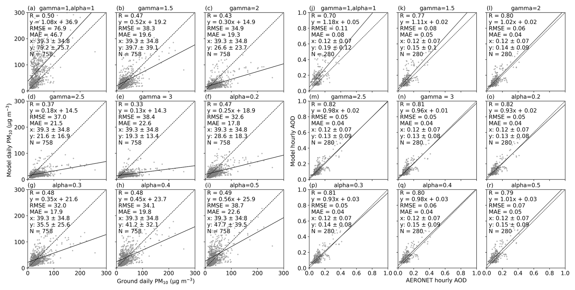
Figure 13 Scatter plot of daily surface PM₁₀ concentration and hourly AOD between model (y axis) and ground observation (x axis) over the dust-prone region of USA-LosAngeles for July 2018. (a)–(i) are for surface daily PM₁₀ and (j)–(r) are for hourly AOD from two groups of sensitivity simulations: (1) gamma = 1, 1.5, 2, 2.5, 3 while alpha stays as 1; (2) alpha = 0.2, 0.3, 0.4, 0.5 while gamma stays as 1, respectively. Also shown on the scatter plot is the correlation coefficient (R), the root-mean-square error (RMSE), the mean absolute error (MAE), the mean ± standard deviation for observed (x) and model-simulated surface PM₁₀/AOD (y), the number of collocated data points (N), the best fit linear regression line (the solid black line) and the 1:1 line (the dashed black line).

Here, we use one month of data to tune the dust emissions by focusing on the magnitude of the total dust load. It is challenging to fine tune each individual dust event and acquire consistent results. The work of Hyde et al. (2018) simulated nine dust storms in south-central Arizona with WRF-Chem using the GOCART AFWA dust emission scheme and the model unevenly reproduced the dust-storm events with some cases overestimating surface PM₁₀ and some cases underestimating surface PM₁₀. Our evaluation of AOD with AERONET observation is rather limited spatially as we only have one AERONET site available over the dust-prone region. We also conduct the same set of sensitivity simulations for July 2019 (results not shown here) and the sensitivities to the tuned parameters are comparable to results shown here in general, which further confirms the validity of the simple approach we have used. Additionally, more recent work has incorporated the albedo-based drag partition (Chappell and Webb, 2016) from satellite data into the GOCART AFWA dust emission scheme to better represent the impacts of roughness features from vegetation and non-vegetation such as soil and rocks, which demonstrated improved model performance in capturing individual dust event over the Southwestern U.S. (LeGrand et al., 2023; Dhital et al., 2024). It is beyond the scope of this work to implement this method, but future work could explore the use of this advanced method and focus on longer periods of model simulation to further evaluate model performances.

4.4 Case study – USA-Atlanta

As described in Sect. 3, for the standard PTA nested domain setup, we have chosen to turn off the cumulus parameterization in the inner domain (D2) with the spatial resolution of 4 km and allow the microphysics scheme to explicitly resolve the convection. Here, we use PTA-Atlanta as an example to examine the impacts of different setups of microphysics and cumulus schemes on model simulated precipitation and surface total and speciated PM_2.5. Since the MAIA satellite mission focuses on speciated PM, we also use PTA-Atlanta here to demonstrate how UI-WRF-Chem simulates speciated PM_2.5 mass concentrations in addition to total PM_2.5.

4.4.1 Impacts of microphysics and cumulus schemes on precipitation and surface total PM_2.5

Southeastern U.S. including the PTA-Atlanta (Fig. 2d) target area experiences pulse-type summer convective precipitation due to the interplay of land-sea breezes, outflow boundaries and complex terrain etc. (Case et al., 2011). Here, we focus on June 2022 over PTA-Atlanta to demonstrate the impacts of different setups of microphysics and cumulus schemes on model simulated precipitation and subsequent surface total PM_2.5 concentration. We perform six UI-WRF-Chem sensitivity simulations with different setups of microphysics and cumulus schemes while keeping other schemes the same as shown in Table 3: (1) mp2cu5: both domain 1 and domain 2 have the Lin microphysics scheme on. Domain 1 and domain 2 have the G3D cumulus scheme on and off, respectively; (2) mp2cu5bothon: same as (1) except that both domain and 1 and domain 2 have the G3D cumulus scheme on; (3) mp2cu3bothon: same as (2) except that both domain 1 and domain 2 have the GF cumulus scheme on; (4) mp10cu5; (5) mp10cu5bothon; and (6) mp10cu3bothon. (4)–(6) are the same as (1)–(3) except that both domain 1 and domain 2 have the Morrison microphysics scheme on. Here, the difference between (1) and (2) illustrates the impacts of turning on/off the cumulus scheme at the 4 km resolution. The difference between (1), (2) and (1), (3) evaluates the impacts of using a traditional cumulus scheme vs. a scale-aware cumulus scheme. Corresponding difference between (1), (3) and (4), (6) represents the impacts of the microphysics scheme.

Table 3 A suite of UI-WRF-Chem sensitivity simulations performed over PTA-Atlanta with different setups of microphysics and cumulus schemes for the outer domain (D1) and inner domain (D2), respectively.

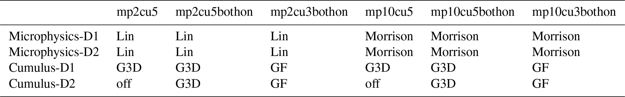
We first focus on the evaluation of daily precipitation. Although, hourly precipitation rate can be important to tell the intensity of the precipitation event, verification of the hourly precipitation can raise double-penalty issues at the finer resolution (Rossa et al., 2008; Gilleland et al., 2009), where a slight shift in the prediction of the timing or location of the precipitation event compared with the ground truth could result in the verification penalties in both space-time. Here, we accumulate the hourly precipitation into daily precipitation to help offset the errors associated with the timing of the event. Figure S15 shows the monthly averaged daily precipitation from UI-WRF-Chem model sensitivity simulations (1)–(6) with surface observations. In general, all the sensitivity runs overestimate the precipitation. Turning on the cumulus scheme in domain 2 when using the traditional G3D scheme results in larger bias compared to the results of turning the G3D scheme off. The work of Zhang et al. (2021) also found that the WRF model had better prediction of precipitation in the central Great Plains in the U.S. when turning off the G3D cumulus scheme with the spatial resolution of 4 km, compared to the sensitivity run of turning on the G3D cumulus scheme. Turning off the cumulus scheme in domain 2 when using the G3D scheme is comparable to the results of the simulation using the scale-aware GF cumulus scheme.

We then investigate the impacts on surface total PM_2.5 concentration. Figure S16 shows the spatial map of surface total PM_2.5 concentration for June 2022 and Fig. 14 compares model simulated daily total PM_2.5 concentration with ground observation. Both sensitivity simulations (2) and (4) with the G3D scheme on for the inner domain (D2) simulate higher precipitation than other simulations, which leads to lower surface PM_2.5 concentrations (Fig. S16b and e). Overall, the surface PM_2.5 concentrations from sensitivity simulations (2) and (4) have the lowest correlation (0.34 and 0.49) compared to other simulations (0.52–0.61) (Fig 14). They also have higher MB (−5.1 and −5.9 µg m⁻³) compared with other simulations (−4.7 to −3.2 µg m⁻³) (Fig. 14). Sensitivity simulations over CHN-Beijing also show similar results related to surface PM_2.5 concentration when contrasting the sensitivity simulation with or without the G3D cumulus on for the inner domain (not shown here). This validates our choice of turning the cumulus scheme off for the inner domain (D2) when using the traditional cumulus scheme such as G3D. When only using the Lin microphysics scheme (mp2), the MAE from simulation (1) mp2cu5 improves on both simulation (2) mp2cu5bothon and simulation (3) mp2cu3bothon (3.7 vs. 5.7; 3.7 vs. 5.1 µg m⁻³) (paired t-test, adjusted p<0.05; Bonferroni correction). When only considering using the Morrison microphysics scheme (mp10), simulation (4) mp10cu5 shows statistically lower MAE than that of simulation (5) mp10cu5bothon (5.0 vs. 6.2 µg m⁻³), while simulation (6) mp10cu3bothon shows statistically reduced MAE than simulation (4) (4.8 vs. 5.0 µg m⁻³) (paired t-test, adjusted p<0.05; Bonferroni correction). Furthermore, simulation (1) outperforms simulation (6) with reduced RMSE (4.6 vs. 5.6 µg m⁻³) and statistically significant lower MAE (3.7 vs. 4.8 µg m⁻³) (paired t-test, adjusted p<0.05; Bonferroni correction). Therefore, we have selected simulation (1) as the final configuration for PTA-Atlanta. It also indicates that surface PM_2.5 concentrations from sensitivity simulations, which turn off the G3D cumulus scheme (1 and 4) are comparable to or even better than the results from the sensitivity simulations (3) and (6), which turn on the scale-aware cumulus scheme GF, although further tests using the GF are needed.

Figure 14 Scatter plot of daily surface PM_2.5 concentration between model (y axis) and ground observation (x axis) over the inner domain (D2) of USA-Atlanta for June 2022. (a)–(f) are the UI-WRF-Chem sensitivity simulations with different setups of microphysics and cumulus schemes. (a)–(c) all have the Lin microphysics scheme on for domain 1. (a) has the Lin microphysics scheme on for domain 2 and no cumulus scheme is used for domain 2. (b) is the same as (a) except that the G3D cumulus scheme is turned on for domain 2. (c) is same as (b) except that the GF cumulus scheme is used for domain 2. (d)–(f) are the same as (a)–(c) except that the Morrison microphysics scheme is used for both domain 1 and domain 2. Also shown on the scatter plot is the correlation coefficient (R), the root-mean-square error (RMSE), the mean absolute error (MAE), the mean ± standard deviation for observed (x) and model-simulated surface PM_2.5 (y), the number of collocated data points (N), the best fit linear regression line (the solid black line) and the 1:1 line (the dashed black line).

There are some uncertainties in this case study. First, our evaluation is limited in time. A longer dataset would be more helpful to reveal model performances in other seasons too (Jeworrek et al., 2021). Also, we have only considered a limited number of model configurations. Previous studies have shown that the prediction of precipitation is also sensitive to other schemes in the model such as the PBL scheme (Klein et al., 2015; Argüeso et al., 2011). Most previous work have focused on the impacts of microphysics and cumulus schemes on precipitation and less have focused on the coupling with the aerosol fields. The process of handling aerosol-cloud interactions would be another source of uncertainty here. Lastly, deficiencies in MERRA-2 meteorology boundary conditions could also introduce uncertainties or biases in the WRF-Chem simulation (Zhang et al., 2021).

4.4.2 Evaluation of model simulated speciated PM_2.5

Surface measurements of total and speciated PM_2.5 mass concentration from the Interagency Monitoring of Protected Visual Environments (IMPROVE) (Malm et al., 1994; Solomon et al., 2014) and the Chemical Speciation Network (CSN) (Solomon et al., 2014) networks (see Fig. S17 for sites location information) are used to evaluate model performance. We compare UI-WRF-Chem simulated speciated PM_2.5 (OC, EC, Sulfate + Nitrate, Dust) and total PM_2.5 against these observations. Figure S18 shows the comparison of daily speciated PM_2.5 between the model and ground observations for the six different sensitivity simulations (Table 3), while Fig. S17 shows the spatial distribution of total and speciated PM_2.5 for the “mp2cu5” sensitivity simulation only.

During this month of June, both surface observations and model simulations indicate that OC, sulfate and dust are the dominate components of total PM_2.5, consistent with previous studies, which show that OC and sulfate are the primary contributors to total PM_2.5 in the Southeastern U.S. (Hand et al., 2024; Zhu et al., 2024). Prescribed burns in the Southeastern U.S. including the states of Alabama and Georgia are a major source of OC emissions in this region (Li et al., 2023; Cummins et al., 2023), some of which are represented by the FLAMBE emission inventory in this work. All the model sensitivity simulations for OC show good correlation (0.45–0.60, Fig. S18) but underestimate ground observations with MB from −1.78 to −1.36 µg m⁻³. Model simulated EC concentrations also show good correlation (0.45–0.72, Fig. S18) but underestimate ground observations with MB from −0.28 to −0.21 µg m⁻³. For the dust component, correlation ranges from 0.42–0.72 (Fig. S18) but all the model sensitivity simulations overestimate ground observations with MB from 0.35–1.53 µg m⁻³. In contrast, the combined sulfate + nitrate for all the sensitivity simulations show relatively lower correlation (−0.03 to 0.23) and underestimate ground observations with MB from −0.71 to −0.35 µg m⁻³. The nitrate concentration from ground observations is low in this region with an average value of 0.198 µg m⁻³ for this month, which makes it challenging for the model to reproduce such a low level. Also due to limited samples used for comparison here, sulfate and nitrate are combined for evaluation. Overall, the “mp2cu5” sensitivity simulation (Table 3) yields the best performance.

Figure 15 shows the variability in total and speciated PM_2.5 mass concentration from model simulation mp2cu5 (Table 3) compared with surface observations as well as the ratio of model simulation to observation. The simulated-to-observed ratio for dust (1–5.8) exhibits much larger variability than other PM_2.5 components (0–2), with model simulation consistently overestimating dust. During this month, PTA-Atlanta may have been affected by long-range transport of Sahara dust in the model simulation. These biases are likely due to uncertainties in the MERRA-2 simulated dust particle size distribution, as also demonstrated by the case studies over CHN-Beijing and ITA-Rome, motivating future work to tune the dust particle size distribution of MERRA-2 data for this region. Ratios for other components mostly remain below 2. Both sulfate and nitrate aerosols are predominantly secondary aerosols in the atmosphere, formed through chemical reactions and are also highly water-soluble, making them sensitive to uncertainties in the aerosol chemistry and wet deposition schemes. As discussed earlier, this month experiences some convective precipitation events, which likely contributes to the uncertainty and large variability in the simulated speciated PM_2.5 concentration.

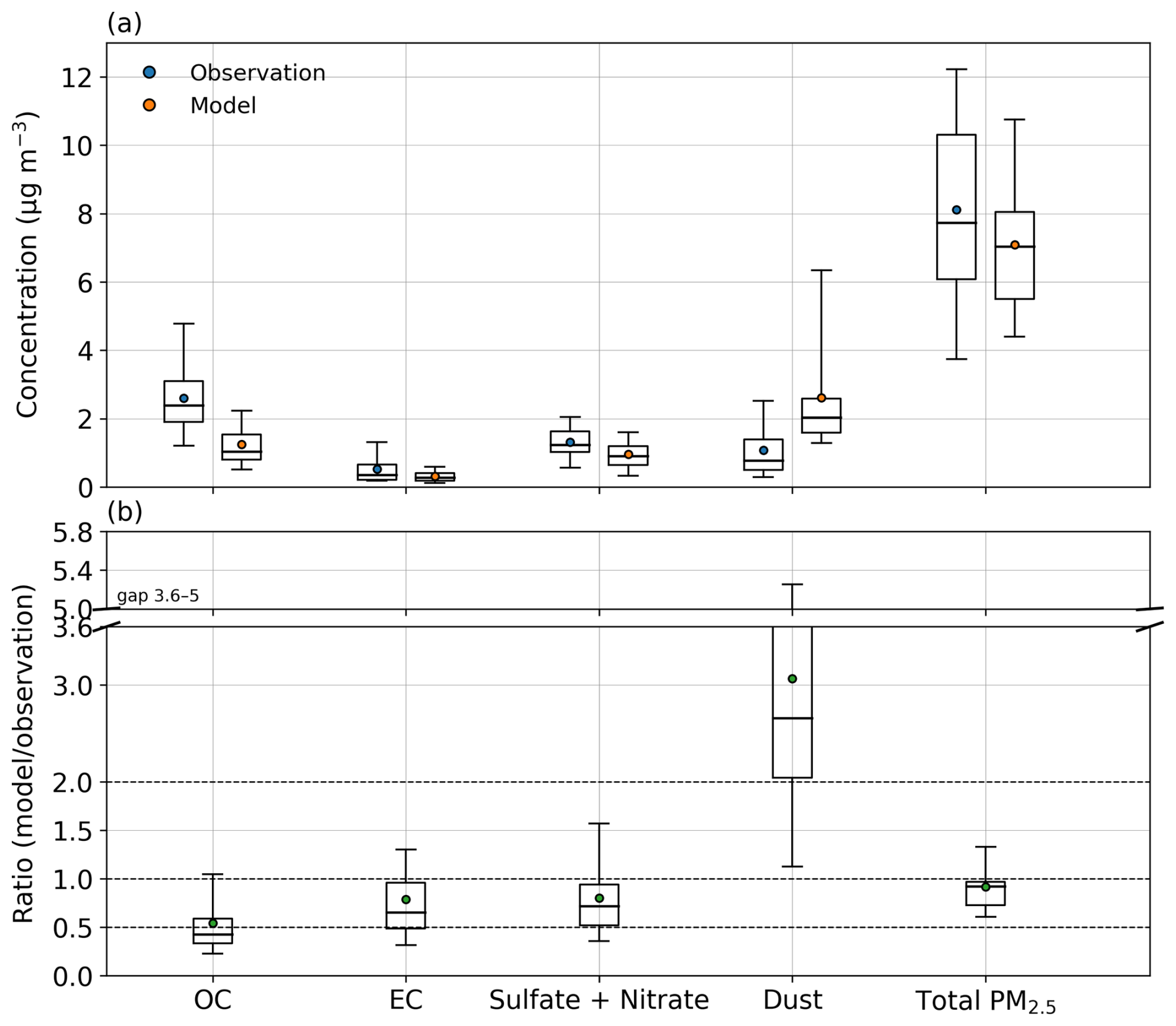
Figure 15 Box-whisker plots of (a) total and speciated PM_2.5 concentrations from UI-WRF-Chem simulation (mp2cu5 in Table 3) and surface observations from IMPROVE and CSN sites over the inner domain (D2) of PTA-Atlanta for June 2022, and (b) the ratio of model simulated to observed PM_2.5. Speciated PM_2.5 include OC, EC, dust and the combined sulfate + nitrate. Also Shown on the boxer plot are the 5th and 95th percentiles (the whiskers), the interquartile range (the boxes), the median (the black lines) and the mean (the filled circles). Note on (b), the y axis is truncated between 3.6–5.0 for improved visualization.

Although our analysis here is limited to one month and one PTA, it provides a valuable case study of how the UI-WRF-Chem modeling framework simulates speciated PM_2.5. Moreover, previous work by Jin et al. (2024) using the same UI-WRF-Chem framework demonstrated its broader robustness over the Boston PTA. It illustrated the feasibility of the MAIA modeling framework for generating L2 and L4 PM products with a full year (2018) of UI-WRF-Chem outputs of total and speciated PM_2.5 mass concentrations and showed the correlation of evaluating model total and speciated PM_2.5 mass concentrations against ground observations ranging from 0.40 to 0.73 (Table S1 therein). Together, these results suggest that while the single-month evaluation such as the case study here only provides a partial picture of model performance, the framework has been shown to produce reliable and robust results for longer time periods. Future work will therefore focus on a more comprehensive assessment of model performance with respect to the PM composition using longer datasets across different PTAs.

5 Conclusions and discussion

We have developed the Unified Inputs (of initial and boundary conditions) for WRF-Chem (UI-WRF-Chem) modeling framework as the CTM, to support the MAIA satellite mission, which aims to study how different types of PM air pollution affect human health. The UI-WRF-Chem outputs including meteorology variables as well as total and speciated PM concentrations will be integrated together with satellite and ground-based observations data to generate surface total and speciated PM maps. Building upon the standard WRF-Chem model, we have developed new modules and included major enhancements in the UI-WRF-Chem framework to improve model simulated meteorology variables, PM concentration and AOD. These major developments include: (1) using NASA GEOS data including GEOS FP and MERRA-2 data to provide both meteorological and chemical initial and boundary conditions to drive WRF-Chem simulations at a finer spatial resolution for both forecasting and reanalysis modes; (2) using a global or regional land data assimilation system (GLDAS or NLDAS) to constrain soil properties (e.g., soil moisture); (3) updating land surface properties (land cover type, LAI, GVF and albedo) with recent available MODIS land data products; (4) developing a new soil NO_x emission scheme – BDISNP; (5) developing the WEPS stand-alone module to process both global and regional anthropogenic emissions as well as fire emissions.

In this work, we focus on four target areas to demonstrate the application of the UI-WRF-Chem modeling framework: CHN-Beijing, ITA-Rome, USA-LosAngeles, and USA-Atlanta. Each target area is set up with 2 nested domains with a 12 and 4 km spatial resolution for the outer domain (D1) and inner domain (D2), respectively. First, we conduct a suite of sensitivity simulations over each target area to select the optimal combination of physics schemes used in the model. We have chosen to turn off the cumulus scheme for the inner domain (D2), since we are using the traditional G3D cumulus scheme, which is not a scale-aware scheme. We investigate the impacts of cumulus and microphysics schemes on model performance over the USA-Atlanta target area for June 2022. Our case study shows that turning on the G3D cumulus scheme in the inner domain (D2) produces higher precipitation than the sensitivity simulation with the G3D scheme off, which in turn leads to lower surface total and speciated PM_2.5 concentrations. Compared with surface observations of precipitation and PM_2.5 concentration, the sensitivity simulation with the G3D scheme off shows better performance than keeping it on. Due to the problem with the scale-aware GF cumulus scheme in the model (not coupled to the chemistry), we are not able to fully investigate the impact of a scale-aware scheme on model performance in the current work. Future work will explore the use of this scale-aware scheme with longer periods of simulation or across different target areas.

Both CHN-Beijing and ITA-Rome target areas are affected by dust long-range transport events. We select two dust intrusion events that impacted these two target areas. A dust storm originated from the Taklamakan and Gobi Deserts around 24 March 2018 and moved downwind to CHN-Beijing from 27 to 28 March 2018. For ITA-Rome, we focus on June 2023, where Saharan dust transported to the target area. For both target areas, we conduct UI-WRF-Chem sensitivity simulations with different chemical boundary conditions from MERRA-2 data being considered: no chemical species; including dust and other aerosols. Here, we develop a method to constrain the dust concentration for each size bin in the MERRA-2 data using AERONET data. We compare the dust PSD from MERRA-2 data with AERONET observations to better distribute the dust concentration in different size bins in the MERRA-2 chemical boundary conditions, based on long-term datasets. Our results show that including the dust and other aerosols in the boundary improve model simulated surface PM concentration and AOD during dust intrusion events for both target areas, compared to the model run without using MERRA-2 chemical boundary conditions. Using the constrained dust concentration in the MERRA-2 data further improves model performance. This method helps reduce the computational cost when long-range transport or regional transport affects a target area. Otherwise, we would need to add a third nested domain with expanded domain size to cover the pollution sources such as the dust source region. Since our work mainly focuses on improving the representation of the dust size distribution in MERRA-2 data, we recognize that other global models such as CAM-Chem may also provide useful information for chemical boundary conditions in different applications. While a comprehensive understanding of how different global models affect WRF-Chem simulations of special events such as the dust long-range transport, would provide valuable insights to the community, our work here demonstrates an efficient way for improving the simulation of dust transport using WRF-Chem.

Updating land surface properties (land cover type, LAI, GVF and surface albedo) with recent available MODIS land data improves model simulated TSK compared with MODIS LST, which is demonstrated over the CHN-Beijing target area for July 2018. This could help better capture the UHI phenomenon, which leads to better simulation of processes that are important for surface PM simulation. For other PTAs, which have experienced rapid urbanization, updating land cover type and other land surface properties with recent MODIS land data can be important since the default datasets used in the standard WRF-Chem model are outdated. We also recognize that we have not investigated the use of an urban canopy model to simulate the UHI effect in the UI-WRF-Chem framework. The newly updated BDISNP soil NO_x emission scheme improves the simulation of NO₂, which subsequently affects surface nitrate. Evaluated against TROPOMI NO₂ VCD, the updated BDISNP soil NO_x emission scheme increases NO₂ VCD, mainly over croplands in CHN-Beijing target area than the simulation using the default MEGAN soil NO_x emission scheme, which is mainly due to the application of fertilizer use. Since ground observations of surface NO₂, O₃, and PM_2.5 concentrations are mostly located in urban areas, we acknowledge that our current work is limited in scope, and additional efforts will be needed to further evaluate the impacts of this updated BDISNP scheme in rural areas. Nevertheless, the launch of the GEMS and the Tropospheric Emissions: Monitoring of Pollution (TEMPO) (Zoogman et al., 2017) satellites will provide good opportunities to further refine the BDISNP scheme. The synergy between MAIA and GEMS/TEMPO will also provide opportunities to evaluate both gas and aerosol composition simultaneously.

We perform a case study over the USA-LosAngeles target area, where we tune dust emissions inside the target area. Southwestern U.S., covering part of the USA-LosAngeles target area are desert regions, which experience dust outbreaks. If we use the default dust emission scheme, the model simulated surface PM and AOD overestimate ground observations. We conduct sensitivity simulations to fine tune the parameters in the dust emission scheme as commonly done in the literature to find the optimal parameter. The case study over USA-LosAngeles together with other case studies give an example of the fine-tuning work we are doing as we continue evaluating and improving model performance.

We also use PTA-Atlanta as an example to demonstrate how UI-WRF-Chem simulates speciated PM_2.5. Overall, model simulated daily OC, EC and dust show higher correlation (0.5, 0.71 and 0.72) while the combined sulfate + nitrate aerosol concentration shows relatively lower correlation (0.23), when evaluated against measurements from IMPROVE and CSN networks. Since our work is based on only one month of data with precipitation events, the simulated total and speciated PM_2.5 concentrations are subject to large uncertainty and variability, particularly due to chemistry and wet deposition schemes associated with precipitation. As a result, this analysis only provides a partial picture of the model performance. Nevertheless, previous work by Jin et al. (2024) demonstrated the robustness of the UI-WRF-Chem framework over the Boston PTA, showing its feasibility for generating MAIA L2 and L4 PM products. Using a full year (2018) of UI-WRF-Chem outputs, they reported correlations of 0.40–0.73 between simulated and observed total and speciated PM_2.5 (Table S1 in the Supplement therein).

The MAIA project leverages existing PM monitoring networks where available and has deployed additional PM speciation monitors in PTAs where such data were otherwise unavailable, including through the Surface Particulate Matter Network (SPARTAN) (Snider et al., 2015). At the time of writing, long-term datasets of speciated PM_2.5 from observations are only available for some PTAs and extended model outputs are not yet available for all PTAs. We have since generated extended UI-WRF-Chem model outputs for each PTA and longer observations of speciated PM_2.5 are being collected. As part of the MAIA satellite mission, these expanded UI-WRF-Chem model outputs will enable a more comprehensive assessment of UI-WRF-Chem model performance, especially for speciated PM_2.5 across diverse PTAs. Such evaluation will enhance the robustness of UI-WRF-Chem for its role in the MAIA satellite mission and provide valuable insights for simulating PM composition in support of air quality and public health studies.