the Creative Commons Attribution 4.0 License.
the Creative Commons Attribution 4.0 License.
 | 24 Nov 2025
The Lagrangian moisture source and transport diagnostic WaterSip V3.2
WaterSip is a diagnostic software tool that identifies the evaporation sources and transport pathways of precipitation or water vapour over a target area based on Lagrangian model output. In addition to the geographic location, WaterSip identifies select thermodynamic properties of the moisture sources, during atmospheric transport, and arrival over the target area based on Lagrangian particle dispersion or trajectory model output. WaterSip software thereby employs the Lagrangian diagnostic algorithm for quantitative moisture source accounting of Sodemann et al. (2008b). Moisture sources are identified from changes in specific humidity along trajectories at each output time step. The ratio between changes in specific humidity and the specific humidity of the air parcel allow to estimate the quantitative contribution of a moisture source to an air parcel at a specific time and location. This contribution and its temporal sequence provides the basis for identifying moisture source contributions to the final precipitation. WaterSip is designed to operate on large datasets of trajectories filling regional to global domains. The results are provided as gridded information in a variety of output files in netCDF format. This paper revisits the relevant methodological foundations, describes the configuration and technical set-up, and provides a consistent example case study to illustrate the use and interpretation of the software tool and its results. A short sensitivity study supports the choice of the main parameters of the diagnostic. Key uncertainties and caveats are described and discussed throughout the text. Users of WaterSip should be aware of these uncertainties to obtain a valid and reliable interpretation of the diagnostic results.
- Article
(11528 KB) - Full-text XML
- BibTeX
- EndNote


Atmospheric dynamics transports water vapour from an evaporation source to a precipitation sink, as manifested in the global spectrum of weather systems. Knowledge about how weather systems shape the atmospheric water cycle from source to sink is key for understanding the causes of hydro-meteorological extremes (e.g., Brubaker et al., 2001; Winschall et al., 2014b; Holgate et al., 2020), precipitation seasonality (e.g., Sodemann and Zubler, 2010; Singh et al., 2017), and climatological averages (e.g., Brubaker et al., 1993). Process studies have for example investigated how oceans contribute to precipitation on land (Stohl and James, 2004), and how land areas recycle precipitation (Eltahir and Bras, 1996; Dominguez et al., 2016). On paleoclimate time scales, knowledge of the variation of sources and transport pathways of water vapour are central to the interpretation of archives of the past hydroclimate, including ice cores (e.g., Johnsen et al., 1989; Sodemann et al., 2008a) and cave deposits at lower latitudes (e.g., Breitenbach et al., 2010; Moerman et al., 2013; Baker et al., 2015).
Measurements of precipitation and atmospheric water vapour do not directly reveal information about their evaporation sources. In specific situations, the stable water isotope composition of atmospheric waters may allow to separate the contribution of different source regions from the effect of phase changes during transport (Sodemann et al., 2008a; Aemisegger et al., 2014; Weng et al., 2021). In general, however, due to the multitude of influences, the problem is underdetermined. Furthermore, the interpretation of water isotope measurements themselves can require additional diagnostic numerical tools to disentangle the contribution of different processes and evaporation sources. As a consequence, results from moisture source studies generally suffer from a lack of definitive, observable constraints.
Different approaches from atmospheric models and model data have been used over time to access information on water vapour's sources and transport conditions (Dominguez et al., 2020). Conceptual studies evaluated the water balance in domains over a given region, for example to determine precipitation recycling over the Continental US (Eltahir and Bras, 1994) and the Amazon region (Salati et al., 1979). Much more complex approaches release water vapour tracers within a numerical atmospheric model's water cycle (Numaguti, 1999; Sodemann and Stohl, 2009). Hereby, water vapour is transported forward within a secondary water cycle of the numerical model for selected 'tagged' subsets of total evaporation. Such tagging approaches require a very substantial computational effort to obtain detailed representation of the sources, and over seasonal to inter-annual time scales. To reduce the computational efforts, Eulerian offline methods with reduced complexity have been developed (Yoshimura et al., 2004; van der Ent et al., 2014). As an intermediate in terms of complexity and computational demand, Lagrangian methods have been employed to diagnose the water budget along air parcel trajectories (Dirmeyer and Brubaker, 1999; Stohl and James, 2004; Gustafsson et al., 2010). Since trajectories can be calculated off-line from stored atmospheric fields, for example reanalysis data, such an approach is computationally more efficient than tagging studies. In addition, Lagrangian methods can more easily provide the spatial extent of moisture sources, and thus provide an intuitive connection between source and receptor areas.
This paper describes the concepts and use of the WaterSip1 software. WaterSip consists of an implementation of the widely used Lagrangian moisture source and transport diagnostic of Sodemann et al. (2008b). WaterSip provides a means to identify and characterise the source regions and transport conditions of water vapour and precipitation from Lagrangian air parcel trajectories. The algorithm of the WaterSip software includes an accounting procedure. This processing step provides quantitative estimates of the moisture source contributions to precipitation (or water vapour) in a target area. This quantitative information can then be used to provide, for example, the average sea surface temperature at the moisture source (Sodemann et al., 2008b), the fraction of land versus ocean surface contribution (Sodemann and Zubler, 2010), the duration and transport distance from evaporation to precipitation (Laederach and Sodemann, 2016), as well as the extent of mixing and rainout during transport (Dütsch et al., 2018). For comparison, the algorithms of Stohl and James (2004), Dirmeyer and Brubaker (1999), and Gustafsson et al. (2010) are also available in the WaterSip tool.
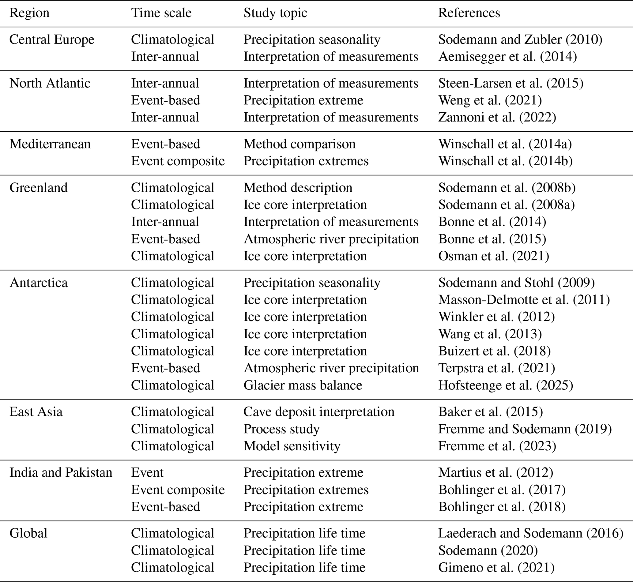
A bibliographic overview of studies that have used the Sodemann et al. (2008b) algorithm with the WaterSip software shows the global to regional coverage of previous work, and the variety of study objectives, from event-scale to climatological studies, process studies, sensitivity studies, and the interpretation of measurements and paleoclimate records (Table 1). Since the original publication of this diagnostic method, numerous technical and conceptual developments have taken place, which are either fragmented across several publications, or not coherently described in the current literature. The main objective of this work is therefore to provide a consistent reference point for the use and interpretation of the method and software, including its wide array of additional diagnostic output of moisture transport characteristics. Users will therefore no longer need to re-implement the diagnostic algorithm behind WaterSip themselves, and can focus on the application of the tool to different subject areas.
Sodemann and Zubler (2010)Aemisegger et al. (2014)Steen-Larsen et al. (2015)Weng et al. (2021)Zannoni et al. (2022)Winschall et al. (2014a)Winschall et al. (2014b)Sodemann et al. (2008b)Sodemann et al. (2008a)Bonne et al. (2014)Bonne et al. (2015)Osman et al. (2021)Sodemann and Stohl (2009)Masson-Delmotte et al. (2011)Winkler et al. (2012)Wang et al. (2013)Buizert et al. (2018)Terpstra et al. (2021)Hofsteenge et al. (2025)Baker et al. (2015)Fremme and Sodemann (2019)Fremme et al. (2023)Martius et al. (2012)Bohlinger et al. (2017)Bohlinger et al. (2018)Laederach and Sodemann (2016)Sodemann (2020)Gimeno et al. (2021)Table 1Previous studies using the Sodemann et al. (2008b) method with the WaterSip software. Studies have been classified by their study region, time scale, and study topic.
The WaterSip software in current version 3.2 described here gives users flexibility in its configuration with regard to different threshold parameters, and gives access to a multitude of additional moisture source and moisture transport characteristics obtained from the algorithm. WaterSip currently works with two common models providing air parcel trajectories (LAGRANTO, Sprenger and Wernli, 2015) and particle dispersion trajectories (FLEXPART, Stohl et al., 2005), and can be extended to read in trajectory files produced from other trajectory calculation tools. Implemented as a C++ code with parallelisation in openMP, and writing output files in netCDF format, the WaterSip code can be easily integrated in common scientific computing environments and workflows.
The paper starts with a overview of the working principle of the algorithm and introduces key quantities (Sect. 2). This is followed by a description of the configuration of a run (Sect. 3), followed by practicalities such as input data, running the software, and an output file description (Sect. 4). A case study is used as a consistent example throughout the manuscript to get users started with the diagnostic output capabilities and the interpretation, providing guidance in applying WaterSip to new research topics. Readers who are new to the method may choose to first look at the description of the results from the example case (Sects. 4.4 and 5) before reading through the method description. Being an off-line diagnostic based on air parcel trajectories, WaterSip makes several simplifying assumptions that introduce uncertainty to the results. Causes of uncertainty are mentioned throughout the text and discussed in Sect. 6. Users are advised to think carefully about the inherent limitation of the method to obtain valid and reliable conclusions from applying WaterSip during their research efforts.
The original publication of the diagnostic algorithm of Sodemann et al. (2008b) was implemented as a set of FORTRAN routines and shell scripts for use with trajectories from LAGRANTO (Sprenger and Wernli, 2015). Since then, there has been a considerable growth in studies with this algorithm (Table 1). Alongside, there have been new conceptual and technical developments that require an updated reference publication. These developments include the use of WaterSip with FLEXPART model output (Sodemann and Stohl, 2009), assessing the role of convection and assimilation increments (Sodemann, 2020; Fremme et al., 2023), the distinction of mixing and rainout events during transport (Dütsch et al., 2018), the analysis of lifetime distribution of water vapour (Winschall et al., 2014b; Laederach and Sodemann, 2016; Sodemann, 2020), interpretation of stable isotope characteristics (Weng et al., 2021), the identification of water vapour in addition to precipitation, as well as technical developments regarding input and output files, configuration and output quantities. This section provides a coherent description of the working principle of the algorithm, including the mathematical formalism that will be used in the remainder of the manuscript.
2.1 Description of the diagnostic accounting algorithm
Generally, the Sodemann et al. (2008b) algorithm used in WaterSip works based on trajectories of atmospheric air parcels, described by a time-dependent coordinate vector x(t) of positions given by longitude λ, latitude ϕ, and height z:
Air parcel trajectories on the way to a target area A (Fig. 1a, black frame) may pass over the underlying surface of either ocean (blue area) or land regions (green area), thereby acquiring moisture at the moisture sources (hatched area). Acquisition of moisture by an air parcel is termed a moisture uptake, and the ensemble of all moisture uptakes to an air parcel then comprises the moisture source. Identifying the relevant set of air parcels arriving over a target domain and their corresponding trajectories is the first step of the Sodemann et al. (2008b) algorithm (Fig. 1c, step 1).
Next, in order to determine the moisture sources of an air parcel, specific humidity q and air temperature T, or relative humidity RH and T, must be available along the same trajectory. These are commonly obtained by interpolation from four-dimensional NWP model output fields. For example, the 4-D specific humidity field Q is used to obtain q(t) along the transport pathway of air parcels towards a target area at every time interval i with time step Δt:
The conceptual starting point of the algorithm is then the Lagrangian water budget, describing the change in specific humidity along an air parcel trajectory resulting from evaporation (e) and condensation (c) (Stohl and James, 2004):
The discretized Lagrangian water budget, giving the change in q along a trajectory with time step Δt of ∼ 1–6 h at time step i is then
The arrival time at target area A is given by t=0 at step 0, and i increases backward in time along the trajectory (Fig. 1d, horizontal axis). The change in specific humidity from the previous interval, i+1, to interval i is then obtained from
Importantly, Δqi can either be positive, zero, or negative (Fig. 1d). A positive Δq (i.e., Δq>0) is interpreted as a so-called moisture uptake, while a negative Δq (i.e., Δq<0) is interpreted as a moisture loss along the trajectory. Thereby, Δqi is always a net effect of both ei and pi that may have affected the water budget of the air parcel during time step i. The algorithm necessarily assumes that either evaporation or precipitation exclusively act on an air parcel during discretisation time Δt, which introduces uncertainties depending on the discretisation time Δt (see Sect. 6). In practice, a critical specific humidity threshold Δqc is used to filter out smaller variations in Δq that are due to numerical noise (see Sect. 3.1, Fig. 1d).
Conceptually, each moisture uptake Δqn along the trajectory path contributes a share Δqn to the arriving moisture q0:
Thereby, qr is a residual amount of moisture that already was present in the air parcel at the earliest available time step of the trajectory with unidentified sources (see Sect. 3.3.3). Due to rainout and mixing effects along the further transport, a part of the uptake moisture can be lost, and Δqn will only contribute with a fraction fn to the moisture at the arrival location:
The objective of the accounting step of the Sodemann et al. (2008b) algorithm is now to obtain an estimate of the contributing fraction fn for each of the U identified moisture uptakes (Fig. 1c, step 2). The moisture accounting provides all fn, which then allow to diagnose where, when, and under what conditions the air parcel water budget changed, and to what extent this is reflected in the precipitation falling from the air parcel (Fig. 1c, step 3).
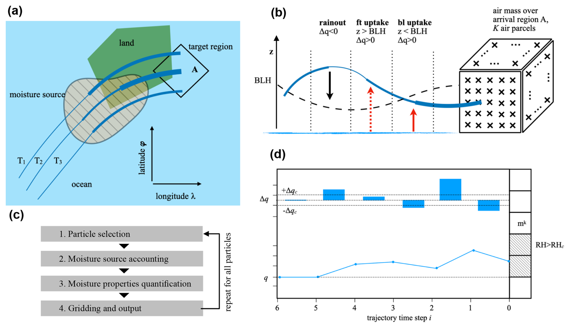
Figure 1Schematic illustration of the moisture source diagnostic. (a) Horizontal view of a bundle of trajectories (, dark blue lines) arriving in a target region A (black frame). The trajectories pass over ocean (light blue) and land regions (green). An area of moisture uptake (hatched, orange) is detected where the specific humidity increases along trajectories (broadening blue lines). (b) 3-dimensional view of an air mass represented by air parcels that are traced backward using trajectories. Crosses denote arrival points in the air mass over the arrival domain A (black box). Locations of moisture increase from evaporation above the boundary layer (dashed red arrow), within the boundary layer (solid red arrow), and decrease from precipitation (black arrow) are detected from changes in the specific humidity along trajectories (width of blue line). Moisture uptakes (Δq>0) can be within the boundary layer (bl uptake) or in the free troposphere (ft uptake). Note that many trajectories at different vertical levels contribute to the Lagrangian precipitation estimate in the arrival region. Dashed black line denotes boundary-layer height (BLH). (c) Flow diagram of processing steps in the WaterSip diagnostic. (d) Schematic of moisture uptakes and losses along 6 time steps of an air parcel with mass mk arriving at grid-scale saturation, identified by RH above a threshold value RHc (shading). Note that some of the specific humidity changes are smaller than a set threshold value for significant specific humidity changes Δqc. See text for details.
At the time of a moisture uptake, the fractional contribution fn for each uptake n is directly obtained from
If at a later time another moisture uptake contributes to the specific humidity in the same air parcel, qn will change, and fn needs to be recalculated to reflect its decreased share. This sequential updating of the fractional contributions is referred to as the accounting of specific humidity along the trajectory. In Fig. 1d, a moisture increase between time intervals 4 and 5, for example, that is larger than the threshold value Δqc, gains a smaller relative share of the arriving moisture q0 after a large uptake occurs between time steps 1 and 2. A more detailed, quantitative example is given in Sodemann et al. (2008b).
In the case of another moisture uptake at a later time step i, the fractions fm of all previous uptakes m>i simply need to be recalculated using Eq. 8 as
In the case of a moisture loss (due to precipitation) at a later time i, some of the moisture contributed from previous uptakes m<i will be lost. Since the Sodemann et al. (2008b) algorithm assumes that the water vapour is well mixed within a given air parcel, precipitation events do not change the fractional contributions at that time. However, a later moisture loss Δqi does remove moisture from previous uptakes Δqm according to their fractional contribution fm at time m:
The accounting is complete when the above steps in Eqs. (7)–(9) have been applied from the earliest time of the trajectory up to the arrival time t=0. Dütsch et al. (2018) compactly expressed the final result of this accounting method in two update equations. While the algorithm is presented here in a detailed representation of each of the computational steps, the equations in Dütsch et al. (2018) are almost entirely equivalent, and may facilitate a numerical implementation of the algorithm (for one exception see below). WaterSip currently implements only this stepwise accounting procedure.
The vertical location of the air parcel as moisture uptakes take place can be used to infer the reliability of the assumption that water vapour stems from evaporation at the current location. If air parcels are within or close the the height of the (well-mixed) boundary layer, this assumption is considered more likely to be valid than if the uptake is detected well into the free troposphere (Fig. 1b, dashed line). The boundary-layer height scale factor sh is used to separate between uptakes considered to be within the boundary layer or within the free troposphere (see Sect. 3.1.4).
2.2 Precipitation estimate
Up to this point, the algorithm has provided quantitative information about the contributions of uptakes to the moisture within an air parcel at x(t=0) at some height z. While it is possible to directly use the information about the sources of the water vapour, more commonly one would be interested in the moisture sources of surface precipitation. In order to transfer the water vapour information to surface precipitation at the arrival point of trajectories, moisture loss from a precipitating air parcel at the last time step before arrival (Δq0<0) is assumed to directly contribute to surface precipitation. To obtain a reliable estimate of the total precipitation in an area, a sufficiently large set of particle trajectories is required to faithfully represent the atmospheric column above a target area (Fig. 1b, crosses). Then, the Lagrangian precipitation estimate (in units of kg m) can be computed as the column integral of all for all K air parcels with mass mk residing over the target area A at time t=0:
To obtain a spatially coherent view, the contribution of each individual air parcel is gridded onto the arrival grid using a gridding kernel (see Sect. 5.3). Thereby only air parcels fulfilling certain requirements are considered in the analysis of precipitation moisture sources. For example, to further support the presence of clouds leading to precipitation, a critical relative humidity threshold RHc is applied, where clouds are assumed when the grid-scale relative humidity exceeds 80 % (see Sect. 3.1.3).
2.3 Accounted fraction
The sum of all fractional contributions from identified moisture uptakes U along trajectory k, the total accounted fraction , provides information about the known sources of and thus :
Hereby, U is the number of all moisture uptake events identified along trajectory k. Based on the vertical position (particle elevation) z where the uptake is identified, the fractional contributions are subdivided into the two categories: the accounted fraction in the boundary layer, , and the accounted fraction in the free troposphere, . The sum of both fractions is the total explained fraction , which should obey the relation
Then, provides information about the consistency of the algorithm. In general, and on average, this relation is found to be indeed fulfilled. However, if the Δqc threshold is set to values outside a meaningful range, the total explained fraction can exceed 1.0. Typically, this will happen for large values of the precipThreshold parameter, which can lead to undetected rainout events (see Sect. 3.1.2). Users are thus advised to inspect in their results and to make adjustments if needed. Notably, this is a difference to the algorithm of Dütsch et al. (2018) where ftot≤1 by definition.
The explained fractions , can be used further to subdivide the Lagrangian precipitation estimate into its respective explained fractions. The total explained precipitation is obtained from
Corresponding quantities and can be computed for fbl and fft. A choice to consider in this respect is which precipitation should be used for the weighted average of diagnosed quantities, or only the explained fractions of (, , ). Given that the Lagrangian precipitation estimate is typically in error by about 20 %–30 % or more (Stohl and James, 2004), this choice might be secondary for the interpretation of the final results. In the Sodemann et al. (2008b) algorithm as implemented in WaterSip, is used, rather than .
WaterSip has a long list of configuration parameters that control the workings of the algorithm. The configuration is supplied as a text-based input file, that consists of sets of parameters, which are organised into thematic sections. This section describes how to control core algorithm parameters (Sect. 3.1), how to handle the discretisation of the arrival air mass (Sect. 3.2), and how to configure the output grids (Sect. 3.4). While the detailed format of the text-based input file is described in Appendix B, the following sections mention the name of the relevant parameters and input file sections, exemplify typical values, and describe relevant findings from the literature along the way. A brief sensitivity study of several key parameters is provided in Sect. 6.1.
3.1 Core algorithm parameters
The core parameters of the Sodemann et al. (2008b) algorithm are a set of threshold parameters that determine the identification of moisture uptakes and precipitation events from the Lagrangian moisture budget along trajectories.
3.1.1 Uptake threshold Δqc
Specific humidity changes along air parcel trajectories are not only reflecting e−p, but also contain spurious noise due to interpolation from gridded NWP output and inaccuracies in trajectory calculations (Stohl, 1998). There may also be an impact from parameterised atmospheric processes, such as convection and turbulence, that act at a time scale shorter than the trajectory time interval, and that are only detected by their residual effects (see Sects. 3.3.2 and 6).
In order to suppress or dampen such noise, the uptake threshold Δqc is introduced in the distinction of evaporation and precipitation events. Specifically, a moisture uptake is identified if Δq>Δqc, while a moisture loss is correspondingly identified if Δq<Δqc (Fig. 1c). The uptake threshold is set as parameter uptakeThreshold in the settings group Diagnostics of the configuration file (Table B3). Thereby, the value must be given per trajectory time step (in ).
At a default value of Δqc=0.2 that is typically used in a broad range of mid-latitude conditions, only relatively substantial uptake events are detected by the diagnostic. In Tropical and sub-tropical regions, a larger threshold value may be suitable, whereas in colder and drier conditions, such as in polar or high-altitude regions, a lower threshold of Δqc=0.1 has been recommended (Sodemann and Stohl, 2009). A lower value for Δqc will lead to the inclusion of a larger part of the noise spectrum as moisture uptakes. A larger number of uptakes in turn leads to a higher chance of discounting previous moisture uptakes, and thus may induce a bias towards more local moisture sources.
As an alternative, WaterSip can be instructed to use a relative threshold value Δqcr. In this case, noise is considered as a relative error, and thus the threshold value is computed at every time step as . The relative threshold value is activated by setting the parameter relativeThreshold =1 in the settings group Diagnostics (Table B3). The value of the uptake threshold is then interpreted as Δqcr (as fraction with unit 1). The impact of this relative threshold option has not yet been tested extensively for different climate zones and events.
In the context of the uptake threshold, it is interesting to consider the impact of data assimilation on the specific humidity of gridded NWP data, such as reanalysis data. Data assimilation methods can introduce non-physical perturbations to the moisture field, the so-called assimilation increment. Assimilation increments are another reason to apply Δqc in the diagnostic. If trajectories are calculated using a model forecast without data assimilation, such as for climate model data, no assimilation increments are present in the gridded fields, and thus less noise would be expected in Δq. Fremme et al. (2023) investigated the impact of different Δqc in CESM and NorESM climate model data compared to reanalysis data, and found quantitative but no clear qualitative differences in the result of the diagnostic that could be related to assimilation increments. Users should thus consider testing lower Δqc when using trajectories based on free-running model forecast data rather than reanalyses.
3.1.2 Precipitation threshold Δqp
Similar to the uptake threshold, a corresponding threshold value exists for the identification of moisture losses due to precipitation along trajectories, the precipitation threshold Δqp. As the same amount of numerical noise can lead to spurious identification of moisture losses as for moisture uptakes, the value of is commonly used in mid-latitudes (Sodemann et al., 2008b), while a lower value such as appears more suitable for polar regions (Sodemann and Stohl, 2009). In general, it is recommended for reasons of consistency to use symmetric settings for the uptake and precipitation threshold. The precipitation threshold is set as parameter precipThreshold in the settings group Diagnostics of the configuration file (Table B3). As the detection of moisture losses along trajectories leads to a discount of the remaining contribution from earlier uptake events, a lower precipitation thresholds can lead to relatively less remote moisture sources. The parameter relativeThreshold also affects the interpretation of the value in precipThreshold as absolute or relative parameter value.
3.1.3 Critical relative humidity threshold RHc
The Lagrangian precipitation estimate is based on moisture losses during the last time step of arriving trajectories. In order to further support that a detected moisture loss is likely due to cloud processes, the critical relative humidity threshold RHc is introduced. If RH0≥RHc or RH1≥RHc, the air parcel is associated with clouds during arrival, and thus any negative Δq is assumed to be due to precipitation. RHc is set as parameter arrivalRHMin in the settings group Diagnostics of the configuration file (Table B3). The default value for RHc is 80 (in units of %), corresponding to a common threshold value in parameterisations of sub-grid cloud cover. Several studies indicate that depending on latitude and predominant weather regime, the Lagrangian precipitation estimate increases with lowering of RHc. Such lower threshold values may be argued for in particular in cold, mixed-phase and ice cloud regimes (Terpstra et al., 2021), and in the case of predominantly convective precipitation, that are not necessarily associated with grid-scale cloud cover (Fremme and Sodemann, 2019). An additional parameter arrivalRHMax in the settings group Diagnostics allows to focus the analysis on a a specified range of RH during air parcel arrival, for example if one would be interested in the source properties of water vapour during cloud-free arrival conditions only (Table B3).
Note that a decrease in specific humidity, detected as a moisture loss, can also be a consequence of mixing with drier air, for example due to dry convection. Moisture loss events that take place in an unsaturated environment, i.e., when RH<RHc at both time steps used to calculate any Δqi are therefore counted and processed as dry mixing events, rather than precipitation events (see Sect. 3.1.2). While these mixing events are written to a different output variable (see Sect. 5.1), the consequences for the accounting of moisture losses is the same for saturated and unsaturated conditions.
3.1.4 Boundary-layer height scale factor sh
Another important parameter is the distinction between uptake events that are detected when an air parcel is within the boundary layer, and when it is in the free troposphere. Since air parcel trajectories are 3-dimensional, uptakes are identified when the parcels are at a given height above ground. Evaporation from the surface is assumed to be most plausibly contributing to the moisture increase in an air parcel location if it is within or close to the turbulently mixed atmospheric boundary layer. This resembles the “footprint analysis” of the lowermost 100–300 m above ground, which is commonly used in atmospheric chemistry applications (e.g., Hirdman et al., 2010). Detrainment and venting of boundary-layer air to the nearby free troposphere is another likely pathway for producing moisture uptakes close to the boundary-layer top. Therefore, and to take into account diurnal boundary-layer height variability and the general uncertainty of boundary-layer height calculations, a boundary-layer height scale factor sh with a default value of sh=1.5 is introduced in the diagnostic. All moisture uptakes that are identified when height (with zh the current boundary layer height) are assigned to the output field category of boundary-layer moisture uptake, while all other uptakes are in the free-tropospheric moisture uptake category (see Sect. 5.1). The distinction between these two categories is also carried over to the accounted fractions (Sect. 5.3), and the forward projection of different quantities (Sect. 5.4). The relative threshold value is set as parameter blhScale=1.5 in the settings group Diagnostics (Table B3).
Studies with the WaterSip methodology have used sh in different ways. While Sodemann et al. (2008b) introduced this parameter to obtain more reliable results, free-troposphere and boundary-layer uptakes have since been observed to commonly overlap spatially (e.g., Sodemann and Zubler, 2010). In a detailed investigation of atmospheric conditions associated with free-troposphere uptakes in the Mediterranean, Winschall et al. (2014a) found that these were connected to deep venting of boundary-layer air to the free troposphere due to moist convection. Furthermore, free-troposphere uptakes are generally the lesser fraction of total uptakes, typically on the order of 20 %–40 % (Sodemann and Zubler, 2010; Laederach and Sodemann, 2016). Several studies have therefore in the past considered both uptake categories jointly, in particular in warmer climates (e.g., Martius et al., 2012; Fremme and Sodemann, 2019; Fremme et al., 2023). Users will have to ultimately decide according to their scientific objectives on how to apply sh, and how to make use of the boundary-layer and free-troposphere uptake categories.
3.1.5 Water vapour diagnostics
In addition to tracing back water vapour that leads to precipitation, WaterSip also allows to identify the source and transport properties of water vapour that resides in the atmosphere within a target area at a given time. If WaterSip is used as a water vapour source and transport diagnostic, rather than a precipitation diagnostic, the gridding weight of each traced air parcel is obtained from the total water mass mw of an air parcel of trajectory k at arrival time t=0, computed as
This water mass is then used to weight different quantities during gridding, instead of the loss of water mass during the last time step (, Eq. 17). Apart from this change, the moisture source diagnostic works in the same way when tracing the sources and properties of precipitation water. The water vapour diagnostic option allows for instance to identify the transport properties of water vapour in regions where no precipitation occurs. The water vapour diagnostic is activated by setting parameter analyzeVapour as 1 in the setting group Diagnostic (Table B3).
3.1.6 Other available moisture source diagnostics
To enable comparison of the Sodemann et al. (2008b) algorithm to other approaches, three additional moisture source diagnostics have been implemented into the software tool. These include the e−p diagnostic by Stohl and James (2004), in which all particles arriving in a region and precipitating are gridded without further distinction according to vertical location, and without accounting. Second, the method of Gustafsson et al. (2010), where the moisture source region is identified as the trajectory segment between the first maximum and the trajectory location where the specific humidity becomes lower than the arrival specific humidity for the first time. Third, the method of Dirmeyer and Brubaker (1999) is available, where the evaporation flux below the trajectory location is continuously accumulated until reaching the value of the arrival specific humidity. In order for this method to work, surface evaporation needs to be available on the trajectory input data. The method of Stohl and James (2004) is included by default in the output files. To select one of the two other diagnostic methods, rather than the Sodemann et al. (2008b) algorithm, the parameter processingAlgorithm in settings group Diagnostics needs to be changed from its default value 0 to a value of 1 for the Dirmeyer and Brubaker (1999) method, and to 2 for the Gustafsson et al. (2010) (Table B3).
3.2 Air mass discretisation
When used to diagnose precipitation origin, air parcels are retained for analysis if (i) they reside within the target region, (ii) during the preceding time step had a specific humidity decrease larger than the precipitation threshold value (see Sect. 3.1.2), and (iii) had a relative humidity within chosen bounds (see Sect. 3.1.3). The geographic location of the target region and the considered time period are therefore fundamental choices for an analysis with WaterSip. Other important elements regarding how the air mass is discretised are the format and length of trajectories, and the time interval between particle locations.
3.2.1 Target region and time period specification
In the WaterSip configuration file, the target region is specified by a set of latitude and longitude bounds, namely the parameters arrivalGridMinLon, arrivalGridMinLat, arrivalGridMaxLon, arrivalGridMaxLat in the settings group Grid (Table B2). The grid spacing of the arrival grid in latitude, longitude increments, is defined by parameters arrivalGridDx and arrivalGridDy in the same settings group.
Moisture transport can be strongly modulated by topography, such as for example over Greenland and Antarctica. In order to focus the analysis on different altitude ranges within the target area, but also on selected ground elevation, several parameters are available in the settings group Diagnostics. The parameters arrivalOroMin and arrivalOroMax allow to only retain air parcels for analysis if they arrive over ground elevations within the two parameters. Similarly, air parcels can be filtered according to their altitude above sea level using parameters arrivalAltMin and arrivalAltMax. In order to include all parcels arriving within a domain, the parameters should be set to a height below zero (e.g., −100 m) for the lower, and a large height (e.g., 50 000 m) for the upper threshold value. The used topography is ingested from the netCDF file specified at parameter orographyFile in settings group Case.
3.3 Time period specification
Another fundamental setting is the start- and end-time of the analysis, regulated by parameters startDate and endDate in setting group Case. Since the analysis proceeds backward from the time of arrival, the start date is larger than the end date. Importantly, in order to obtain results for, e.g., 20 d accounting along a trajectory, the time difference between start date and end date must be at least 20 d plus one time step (to enable calculating the required number of specific humidity changes). The length of the analysis period is defined by parameter trajPoints in settings group Case, and the duration of the entire accounting period for each trajectory is then given by the parameter timeStep times trajPoints (see Sect. 3.3.3).
3.3.1 Trajectory input data
Trajectory input data consist of the vectors xk with position and other necessary variables for the K air parcels representing the air mass over the target region (Fig. 1b, box). Such trajectory data can be obtained from different modelling tools. Currently, WaterSip is able to handle input from the Lagrangian trajectory model LAGRANTO (Sprenger and Wernli, 2015), and from the Lagrangian particle dispersion model FLEXPART (Stohl et al., 2005; Pisso et al., 2019). Minimum requirements with regards to the variables that are included on the trajectories are position, T, and q or RH. The input data parameters are set in either settings group Lagranto (Table B7) or Flexpart (Table B6), depending on the used trajectory model.
An important user choice for the WaterSip diagnostic is the discretisation of the atmosphere above the target region into individual particles. In general, the more particles represent a particular air mass, the smaller the mass of air associated with one air parcel (mk), and the more detailed and statistically reliable the results will become. For example, Sodemann and Stohl (2009) used the global FLEXPART dataset of Stohl (2006) from a global domain-filling run with 2.4 million air parcels. With a total global atmospheric mass of 5.14×10¹⁸ kg, each air parcel represents 2.14×10¹² kg of air. Laederach and Sodemann (2016) used 5 million air parcels, resulting in a particle mass of kg. For FLEXPART input data, the particle mass is set by parameter partMass (in kg) in the settings group Flexpart (Table B6).
When using LAGRANTO for the trajectory calculation, the atmospheric mass of one air parcel results from the calculation start grid. For LAGRANTO input data, the particle mass is first computed from the chosen discretisation as
with Δp in units of hPa and Δx, Δy in units of km. Then, is set as parameter partMass (in hPa km2) in the settings group Lagranto (Table B7), which is then internally in WaterSip converted to units of kg. For example, Sodemann et al. (2008b) computed backward trajectories from a 50×50 km horizontal grid over Greenland, with a vertical spacing of 25 hPa for every 6 h time step over a given time period. Accordingly, each trajectory on this grid represents 680×109 kg of air arriving at a specific time interval.
3.3.2 Trajectory time interval Δt
Another important property of the input trajectory data for the Sodemann et al. (2008b) algorithm is temporal discretisation, i.e., the time interval Δt at which meteorological and position information from air parcel locations is available. Typically, Δt corresponds to the time interval of NWP boundary data used during the trajectory calculation. For global reanalyses a common interval is 6 h, but also 1 to 3 h time intervals have been used (Fremme et al., 2023). While trajectory location accuracy increases with a higher input data frequency, there are also potential complications from higher time-resolution input data. As Δqc is well-tested for Δt=6 h with regard to separating signal from noise, smaller threshold values need to be used at shorter time intervals, which do not necessarily have the same filtering effect (see Sect. 3.1). The trajectory time interval Δt is set as parameter timeStep (unit h) in the settings group Case (Table B1).
In a sensitivity study with WaterSip and FLEXPART using climate model data at 1.8×1.8° resolution as input, Fremme et al. (2023) found that the time interval influenced the moisture source distance, with substantially smaller moisture source distances for time intervals of less than 6 h. In that study, the authors then chose to compute trajectories at a time resolution of 1 h to obtain smaller position errors, while the WaterSip diagnostic was run at 6 h time interval to obtain the desired filtering of interpolation noise. With such a combination of time intervals, a compromise can be obtained between trajectory accuracy and sufficient separation between signal and noise in the WaterSip diagnostic.
3.3.3 Trajectory length L
One important consideration for computing trajectories is the trajectory length L, the number of time intervals over which the air parcel movement is traced. Typical trajectory lengths in atmospheric analyses are 5–20 d. Since trajectories become increasingly uncertain for longer calculation time (Stohl, 1998), the trajectory length is an important consideration for WaterSip applications. In the approach of Stohl and James (2004), the results were strongly dependent on the chosen integration time intervals. This choice introduces a subjective element in the analysis, since results may not only vary with climate region, but also with seasons and weather systems. The accounting algorithm implemented in WaterSip does not require a pre-defined trajectory length for its analysis. The trajectory length is set as the number of time steps along a trajectory as parameter trajPoints in the settings group Case (Table B1). One obtains the value of trajPoints from dividing L by Δt. For example, 20 d trajectories with a 6 h time interval results in trajPoints set to 81.
The often-cited global mean residence time of water vapour of 8–10 d (e.g. Trenberth et al., 2007), as obtained from a global budget of atmospheric water vapour and precipitation fluxes, can provide some guidance on how long trajectories need to be. Recent studies (based on Lagrangian moisture source diagnostics with WaterSip) provide arguments that the residence time, or life time of water vapour, may be better described by a heavily skewed life time distribution with a median value of about 4–5 d and a very long, thin tail at 20 d and beyond (Sodemann, 2020; Gimeno et al., 2021). According to these findings, many relevant moisture uptakes can therefore take place within a time scale of 10 d before precipitation. Except at high latitudes, where life times are particularly long, source contributions from the Sodemann et al. (2008b) algorithm are generally not sensitive to a trajectory length beyond 15 d. Using the WaterSip diagnostic with trajectories of 10, 15, or 20 d length will therefore lead to relatively less differing results than with the Stohl and James (2004) method. A generally recommended choice of trajectory length that also allows for the detection of long-range transport of water vapour is 20 d.
3.4 Output grid and output configuration
WaterSip uses the mass represented by each air parcel to transfer the results of the diagnostic onto a grid which will then be written to an output file for further use. There are two output grids in WaterSip. The coarser source and transport grid covers the entire potential source regions of the traced moisture, and is typically of hemispheric or global dimensions. The typically smaller arrival grid covers the target region of the analysis, and usually has a finer grid spacing to reveal spatial details within the arrival domain.
Both grids are specified by a respective set of parameters in the setting group Grids (Table B2). The source grid is defined by the parameters sourceGridMinLon, sourceGridMaxLon, sourceGridMinLat, sourceGridMaxLat, which provides the boundaries in latitude-longitude coordinates. The parameters sourceGridDx, sourceGridDy set the grid spacing in longitude and latitude direction, respectively. A corresponding set of grid parameters exists for the arrival grid (arrivalGridMinLon, arrivalGridMaxLon, arrivalGridMinLat, arrivalGridMaxLat, arrivalGridDx, arrivalGridDy).
Quantities are gridded onto both grids using weighting factors. The weight for gridding a quantity ξ (for example the air temperature at the time of arrival) is obtained from the water mass lost from an arriving air parcel k as
With K trajectories arriving as a vertical stack (Fig. 1b), the weighted average of all ξk at a location λ,ϕ is thus obtained as
This arrival point information needs to be transferred onto the arrival grid. Instead of simply gridding the information to the grid cell closest to the air parcel location, WaterSip allows to specify a spatial representativeness of this information, which is then used to distribute it to surrounding grid cells. Representativeness is provided by a gridding radius rg, specifying a circular distance from the arrival point. The areal overlap between the circular weight and neighbouring grid cells are then used as weights to distribute air parcel quantities ξ onto the arrival grid. For example, with trajectories computed at a horizontal distance of 50×50 km, quantities can be assumed to be representative for a circular area with radius 30 km. If the arrival grid for this setup is then chosen to be arrivalGridDx = arrivalGridDy =0.25°, and the gridding radius is set to rg=30 km, one can expect to reveal finer interpolated structures within the arrival domain. The gridding radius is set as parameters arrivalGridRadius in settings group Grids. Corresponding reasoning applies to the source grid radius sourceGridRadius. Here, a common combination for a hemispheric output grid is sourceGridDx = sourceGridDy =1.0°, and sourceGridRadius =110 km.
The gridding proceeds by finding the area overlaps between the circular gridding area and each grid box. A corresponding fraction of the total quantity to be gridded is then added to each grid box (Škerlak et al., 2014). It is important to be aware of the impact user choices have on the results. A too small gridding radius for a given grid will lead to gaps between grid points, while a too large gridding radius will cause smoothing and potentially loss of detail in the gridded fields.
A final choice regarding the gridding is whether uptake events are gridded with the time stamp of the arrival in the target region, or to the time when uptakes take place. The choice of the assigned time is important for later analysis of the results. In the first case, moisture sources are valid for all precipitation arriving within a chosen time period in the target area, and can be compared to other quantities regarding the arrival time. In the second case, the moisture sources can be compared to properties at the source regions during valid time, for example total evaporation fields. The assignment time is set as parameter assignToUptake in settings group Grids, where 0 denotes that the uptakes are assigned to arrival time, and 1 denotes assignment to uptake time (see Sect. 5.1 for an example).
In order to run the WaterSip diagnostic, a set of suitable input data needs to be available. In this preparatory step of the moisture source analysis, users need to make a number of necessary and optional choices as detailed below. Running the WaterSip tool then produces a set of output files in netCDF format, which are also described in this section.
4.1 Creating and reading trajectory input data
There are some general considerations for the input data to be made such that the WaterSip diagnostic output becomes representative for the chosen target area. The setup for creating trajectory input data to WaterSip varies depending on whether a particle dispersion model (FLEXPART) or an air mass trajectory model (LAGRANTO) is used.
When using the particle dispersion model FLEXPART, commonly, hemispheric or global domain-filling forward simulation are set up. In domain-filling mode, FLEXPART automatically discretises the air mass over the chosen target area into a specified number of particles of equal mass, and distributed according to pressure. With a larger number of particles, WaterSip will provide statistically more robust results, in particular for more long-range and long-duration water vapour transport. Within FLEXPART, particles are advected forward continuously for the simulation time. WaterSip then extracts a sub-set of these trajectories according to the run parameters. A global domain-filling setup has also been applied in the example case presented here (Sect. 4.4). So-called particle dump needs to be activated in FLEXPART to obtain the input data needed by WaterSip. Writing out additional variables with each particle position requires modification of the routine partoutput_pos.f90 or partoutput_short.f90 of the FLEXPART code. Example code for this modification for FLEXPART versions 8.2 through 10.4 is available in the online supplement (Sodemann, 2025a).The most recent version 11 of FLEXPART (Bakels et al., 2024) writes particles in netCDF output. Until WaterSip has been enabled to ingest this input directly, users will have to convert the FLEXPART version 11 particle dump from netCDF to the binary format. A corresponding helper tool is planned to be made available on the WaterSip respository. Running FLEXPART in backward mode can be a more efficient alternative to a global domain-filling run, but requires a new release interval to be defined for every time step. General instructions for setting up and running FLEXPART are available in the respective literature (Stohl et al., 2005; Pisso et al., 2019; Bakels et al., 2024).
When used together with FLEXPART input, the WaterSip configuration file needs to contain a setting group Flexpart, where several parameters need to be specified (Table B6). The parameter particleMass contains the mass per particle as either specified in the FLEXPART releases file, or as written out by FLEXPART in domain filling mode in the output file part_mass. The input files need to be contained in a folder specified by parameter inputDir in setting group Case in the configuration file. As individual particle dump files are read in from FLEXPART output for each time step, the pathname is specified with a wild card pattern (%s) representing the date string, e.g. inputDir = /path/to/directory/partoutput_pos_%s.
When using output from a trajectory model, such as LAGRANTO, the air mass over the target area needs to be discretised manually. This is achieved by defining the start locations of the trajectory calculations in LAGRANTO's startf file. One common way to discretise a target region is to define a regular distance spacing in projected coordinates (e.g., one starting point every 25 or 50 km in both directions). In the vertical, it is recommended to space the starting points at equal pressure intervals. This way, each air parcel trajectory represents an equal amount of mass, which can be entered in the configuration file for a LAGRANTO setup as described earlier (Eq. 16 and Sect. 3.3.1).
It is recommended to run the LAGRANTO program caltra with the flag “-j” to prevent trajectories from intersecting with topography. WaterSip currently only works with the text-based output format of LAGRANTO. Since trajectory variables such as air temperature and specific humidity can be at any column in these files, the column number for each variable needs to be specified explicitly in the configuration file as parameters (Table B7). The input path for LAGRANTO trajectory files is again specified using parameter inputDir in setting group Case of the configuration file, using a file name pattern with wildcard %s to match trajectory files to the desired date range.
4.2 Running the WaterSip diagnostic
The WaterSip code is written in the programming language C. A sample makefile is included with the code repository (https://git.app.uib.no/GFI-public/watersip, last access: 20 November 2025) (Sodemann, 2025b) to compile the program code, and that users may adapt to their computational environment. Installed netCDF, netCDF-C, and netCDF-C4 libraries are in addition required to compile the program code. Lightweight parallelisation has been included by means of OpenMP directives in the code, but compiling with OpenMP is optional. Results of some performance tests are described in Sect. 6.4.
After compiling WaterSip, the input files need to be made available from an external source, such as running FLEXPART or LAGRANTO. The input data and configuration file for the test case in Scandinavia presented throughout this manuscript is available as a supplement to this manuscript (Sodemann, 2025a). A script is included with the test dataset that sets up a recommended directory structure to run WaterSip. Users are invited to experiment with the test case before creating their own setup to get familiar with the usage and output from WaterSip. When running an own case, the directory names for input and output data need to be specified in the configuration file. Then, all other configuration file settings, such as the time period, the target region, diagnostic parameters, need to be set by the user. Importantly, the sections in the configuration file specific for the used input data need to be included and edited to match the input data (Tables B6 and B7).
To start a diagnostic run, the compiled WaterSip program is then executed from the command line. The name of the configuration file is the only argument that needs to be provided when WaterSip is started. WaterSip then starts executing, and provides either output to the terminal about the progress of the analysis, including a time estimate until completion, or an error message that will give an indication how the setup and configuration file need to be adjusted.
4.3 Output files
When a diagnostic run completes, a set of output files is written to the file location specified as parameter outputDir in the configuration file setting group Case. The main output files, containing gridded fields and time series for different averaging times (time step, daily, monthly, annually, all), are created in netCDF format (Table 2). In particular the grid files for days and time steps can become rather large for longer runs. The creation of gridded output files for selected averaging times can therefore be deactivated by setting the respective parameters in parameter set Output from 1 (true) to 0 (false, see Table B5). The series files for different intervals contain time averages of the gridded fields, characterised by the precipitation-weighted mean of each quantity, the unweighted standard deviation, and the minimum and maximum values in the grid area. A sectorisation of the results into user-specified latitude/longitude regions are also contained in the series files (Sect. 5.7). Further output files comprise histogram files (Sect. 5.8) and trajectory files (Sect. 5.9).
Table 2Description of the available output files in WaterSip, including file format, and file name semantics.
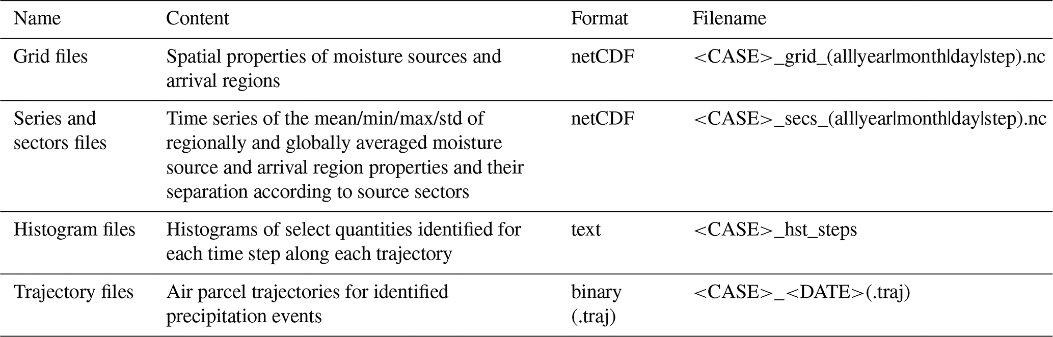
Which variables are contained in the output files can be controlled by the parameters in setting group Variables in the configuration file (Table B5). Output variables are included in the output by setting the corresponding parameter values from 0 to 1. Users can also choose to include static fields, such as topography or the land-sea mask using parameter staticFields. The choice in the setting group Variables affects both grid and series files. If output is activated for variables that are not contained in the input file, WaterSip calculates these from the available information if possible, and otherwise fills in missing values during output. Finally, WaterSip can optionally write out air parcel trajectories in a compact binary format to inspect the result of the moisture diagnostics in detail for individual air parcels (Sect. 5.9).
4.4 Example run configuration
To exemplify the use of the WaterSip diagnostic, a case study for a 10 d Northern Hemisphere summer period (5 to 15 August 2022) over Scandinavia is now presented. The weather situation during the period was characterised by westerly flow, which was steered to higher latitudes by a high pressure system over Eastern Europe. This flow configuration brought several low-pressure systems from the North Atlantic from southwesterly directions towards the Norwegian coast and land areas downstream, which then shed precipitation over Scandinavia.
In order to obtain the required input data for the WaterSip diagnostic, the FLEXPART particle dispersion model in Version 10.4 was run with input fields from the ERA5 reanalysis for a Northern Hemisphere domain with 10 000 000 particles in domain filling mode. The simulation was initialised on 00:00 UTC on 15 July 2022 and run forward for 31 d until 00:00 UTC on 15 August 2022. FLEXPART particle output files (see Data availability section) contain latitude, longitude, height, air temperature, specific humidity, boundary-layer height, and air density at each particle's location, as well as skin temperature, 2 m specific humidity and topography height below the particle. WaterSip was then configured to identify the moisture source and transport properties for a time period of 10 days (5 to 15 August 2022) in the region 54–71° N and 4–32° E. A 6 h time step, 20 d backward tracing, and threshold parameter values RHc=80 and Δqc=0.2 were used for identifying moisture uptakes and losses along the trajectories. Output was activated for all available variables and time steps. The WaterSip setup and output files for this example run are available with the sample data (Sodemann, 2025a).
The following sections describe the different output fields that characterise and quantify conditions at the moisture source, during moisture transport, and during the arrival of the moisture as part of the output. The results and interpretation are thereby exemplified using the case study setup over Scandinavia as described above.
5.1 Moisture source quantities
The most fundamental result of the moisture source diagnostic are the moisture sources, that is the spatial distribution of the moisture uptakes that contribute to precipitation in the target region. Figure 2 shows an example for the total moisture sources of precipitation in a arrival domain over Scandinavia (yellow frame). This moisture source area (shading) may be interpreted as the subset of all evaporation at the moisture sources that ends up as precipitation in the target region. The units of , also corresponding to mm d−1, are obtained from gridding the contribution of moisture uptakes to precipitation in the target region (fi⋅Δq0). When integrated spatially, taking the area of each source grid box into account, one obtains the total precipitation mass in the target area during this time interval. If divided by the target area, the precipitation rate for the analysis period then corresponds exactly to the value of the Lagrangian precipitation estimate (see Sect. 5.3).
In the example case, the largest contributions to precipitating water come from southern Scandinavia and the western North Atlantic, but the moisture sources also stretch into Central and Eastern Europe (Fig. 2a, grey to red areas). In addition, a large area is covered by moisture uptakes with 0.25 mm d−1 or less (blue shading), reaching deep into continental North America. In the example here, the gridding radius on the global maps with a 1.0 × 1.0° spacing was set to 120 km (see Sect. 3.4). A coarser grid spacing and a larger gridding radius would give more smoothed output fields. It is important to consider that a large area with relatively small contributions can still be an overall important moisture source. To quantify the overall contributions for different areas, the source contributions can be averaged within predefined geographic sectors (Sect. 5.7).
The interpretation of moisture source maps can be greatly facilitated in a percentile representation (Fremme and Sodemann, 2019; Fremme et al., 2023). This can be obtained by determining, for example, the 50th and 80th percentiles of the accumulated moisture source contributions, sorted from largest to smallest grid point values. Such a percentile representation is particularly helpful to compare the shape of a moisture source footprint across different events or seasons. In this example case, the 50th and 80th percentile contours for the total moisture source footprint (Fig. 2a, solid and dotted red lines) highlight that almost half of the precipitation is contributed by areas bounded by the orange shading (contour value 0.06 mm d−1), and the large majority is bound by the light blue area (contour value 0.24 mm d−1).
The moisture source detection algorithm distinguishes between uptakes that take place within or close to the boundary layer top, and those that are in the free troposphere, above the boundary layer. For the example case, the moisture sources in the boundary layer dominate (Fig. 2b), while the free-troposphere moisture sources supplement the boundary-layer uptakes over the North Atlantic and Central Europe (Fig. 2c). The collocation of free-troposphere and boundary-layer sources for this event suggests that boundary-layer air may have been vented, moistening the free troposphere. The interpretation could therefore for this case focus on the total moisture uptakes (Fremme et al., 2023).
The moisture source footprint is here compared to the result of the Stohl and James (2004) method for the same case (Fig. 2d). The vertical integral of e−p of all the particle trajectories over 10 d (the quantity (e−p)20 d introduced by Stohl and James (2005) shows patches where evaporation dominates (red shading) and where precipitation dominates (blue shading). While evaporation regions dominate further away, precipitation overcompensates north of Iceland and over the arrival domain, masking potential evaporation from these regions. The presence of such compensating effects, as well as the strong dependency on a selected time scale (not illustrated here), are two of the most important differences compared to the results from the Sodemann et al. (2008b) algorithm. The red contours, indicating the 50th and 80th percentile of total moisture sources from WaterSip, further underline the differences between the results from the two methods.
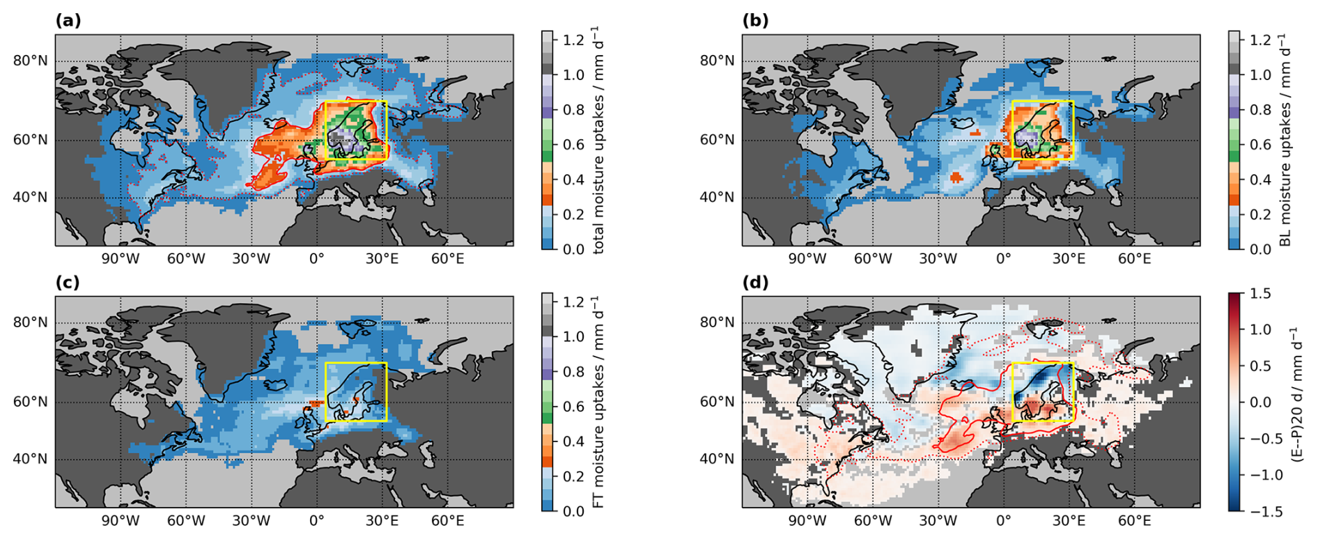
Figure 2Source grid quantities identified for the case study period in 2022. (a) Total moisture uptakes (shading, mm d−1), (b) Boundary-layer moisture uptakes (shading, mm d−1), (c) Free-troposphere moisture uptakes (shading, mm d−1), (d) Lagrangian evaporation minus precipitation budget over 20 d ((e−p)20 d in mm d−1, shading), following Stohl and James (2005). Red contours indicate the 50th (solid) and 80th (dotted) percentile of the total moisture uptakes from WaterSip. Yellow box denotes the target region over Scandinavia. Regions with moisture uptakes of less than are masked out.
In addition to providing the moisture source footprint for an entire analysis period, the WaterSip diagnostic provides gridded moisture sources for each time step in the steps grid file (Sect. 4.3 and Table 2). At 06:00 UTC on 10 August 2022, the precipitation in the target area was sourced from a rather large banded region stretching across the North Atlantic, and reaching into Eastern North America (Fig. 3a). This map shows the moisture uptakes corresponding to precipitation on that day in the arrival region. If one wants to compare the moisture uptakes directly with, for example, gridded evaporation fields, one can use the parameter assignToUptake (Sect. 3.4). The corresponding plot for uptakes on 06:00 UTC at 10 August 2022 shows all evaporating moisture at the synoptically valid time, irrespective of when it will precipitate over the target area. In the given example, relevant uptakes at that time are detected south of Iceland, over Scandinavia, and over western Eurasia (Fig. 3b). The moisture from uptakes at that time will end up as precipitation over the target area at a later time.
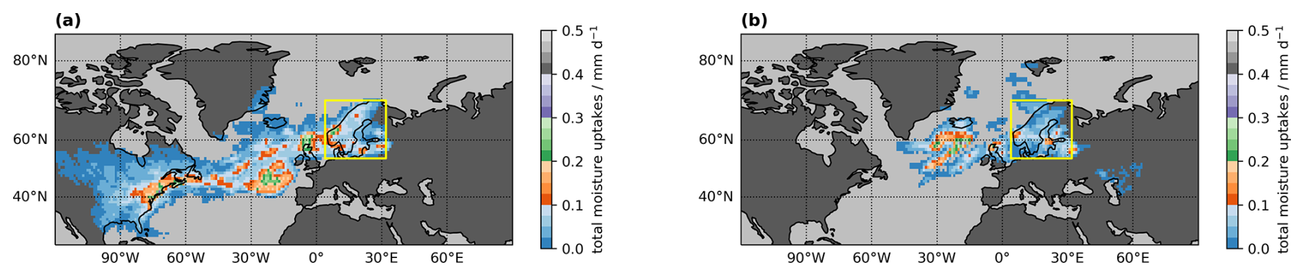
Figure 3Instantaneous snapshot of source grid quantities identified during the case study period with different assignment times. (a) Total moisture uptakes arriving in the target area on 06:00 UTC at 10 August 2022 (shading, mm d−1), (b) Total moisture uptakes taking place on 06:00 UTC at 10 August 2022 (shading, mm d−1). Yellow box denotes the target region over Scandinavia.
5.2 Transport quantities
A number of additional quantities that are indicative of the moisture transport conditions can be obtained on the same grid as the moisture source information. These so-called transport quantities can support the interpretation of the obtained moisture sources in various ways.
The transport pathways of air parcels towards the target region are visible from the particle mass density (Fig. 4a). The particle mass density is an integral of the pathways of all particles' mass bound to the target region in a given time interval. It is obtained by gridding for all time steps of a trajectory. The example case shows the relatively large overall area from where air parcels originate in a 20 d time frame, and the important role of Greenland's topography for guiding the air parcel transport. The quantity “moisture transport” shows the water vapour movement in these air parcels towards the target area. The moisture transport field is obtained by gridding the water mass in tracked air parcels on the way to the target area using for each time step. For the example case, the moisture transport map highlights a dense area of moist air west and south of the target area, and where the moist air crosses the North Atlantic and advances towards the target area (Fig. 4b). This map can be interpreted as a share of total column water bound to the Scandinavia domain. In combination, these two transport quantities allow one to assess the main pathways of air mass transport and the differences to moist air advection to the target region.
Decreases of specific humidity in air parcels during transport can be due to either precipitation events or mixing with drier air (Sect. 2). The moisture rainout field contains the amount of humidity lost from trajectories that are identified when RHi≥RHc from the diagnostic, gridded using Δqi⋅mk along each trajectory. In the example case, moisture rainout events are concentrated over the arrival domain and narrow transport pathways over the North Atlantic and east of Greenland (Fig. 4d), probably related to precipitation formation in air masses that ascend as they approach the target area. In contrast, mixing events are identified as moisture decreases if RHi<RHc, and also gridded using Δqi⋅mk. Both quantities are therefore easy to relate to the (e−p)20 d field (Fig. 2d). For the present example case, air mass mixing is mostly identified over continental North America and over Central Europe (Fig. 2c). It is interesting to note that for this case only a small part of the events are classified as mixing, while the large majority are rainout events. Note that it does not make a difference to the source identification and accounting whether a specific humidity decrease is classified as a mixing or as a rainout event.
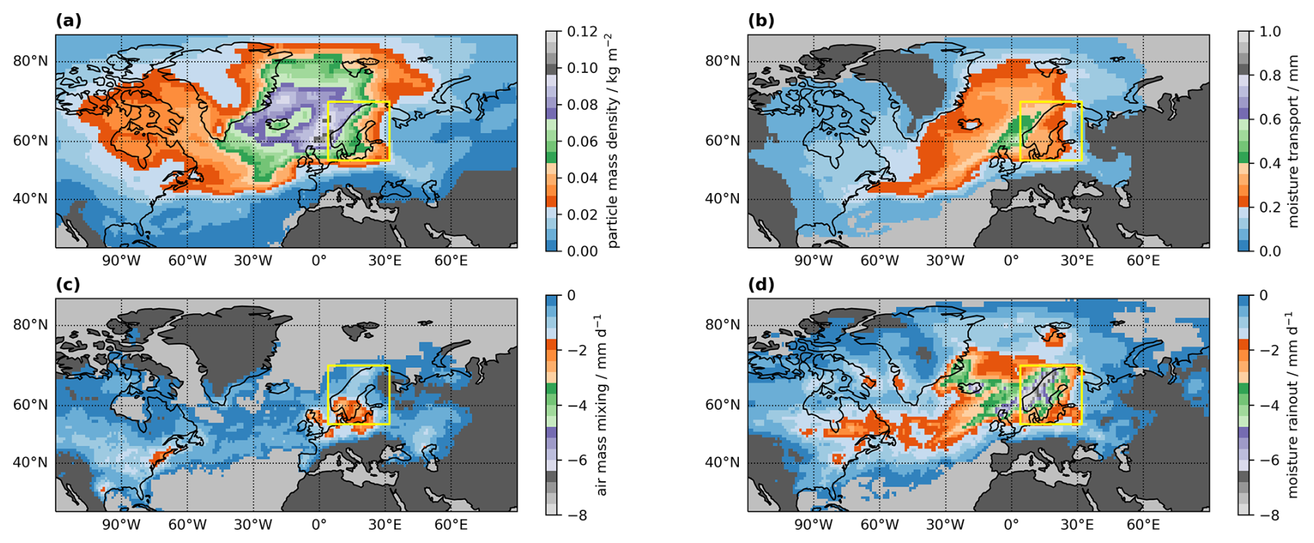
Figure 4Transport quantities identified within air masses bound to the target region for the entire case study period. (a) Particle mass density (shading, kg m−2), (b) moisture transport (shading, mm), (c) air mass mixing (shading, mm d−1), (d) moisture rainout (shading, mm d−1). Yellow box denotes the target region over Scandinavia.
5.3 Moisture arrival quantities
For larger target areas, there can be spatial differences in the atmospheric conditions during air parcel arrival within the domain. It can be interesting to investigate different quantities that are connected to the arrival of air parcel trajectories. These quantities are termed here arrival quantities.
One of the most important arrival quantities is the Lagrangian precipitation estimate (Sect. 2.2). In the example case, there are clear distinctions between the coastal regions of western Scandinavia with an estimated precipitation of above 6 mm d−1, and large parts of the Baltic Sea, southern Sweden and Finland with below 2 mm d−1 during the case study period of 5–15 August 2022 (Fig. 5a, shading). The diagnosed precipitation pattern corresponds qualitatively to ERA5 simulated precipitation during the period (white contours), even though the domain average during the period is about 25 % larger in ERA5 (2.43 mm d−1 compared to 2.07 mm d−1). A direct comparison of the two fields shows that is more smoothed out compared to the sharper pattern in ERA5 (Fig. A1). Regions with high approximately correspond to locations where more air parcels arrive that precipitate according to the selection criteria, as reflected by the arrival count (Fig. 5d). In regions where only few air parcels contribute to arrival quantities, gridded results may show large spatial variations that are not statistically robust. The arrival count can be used for masking such grid points.
Another set of important arrival quantities are the accounted fractions (Sect. 2.3). The total accounted fraction in the example case is uniformly above 95 % (Fig. 5f). Subdividing this quantity into the fractions accounted for by boundary layer uptakes (Fig. 5d) and free troposphere uptakes (Fig. 5e) shows a uniform split into approximately 60 %–70 % boundary layer and 30 %–40 % free troposphere contributions. These shares appear consistent with the corresponding moisture source maps (Fig. 2b, c).
In addition, some thermodynamic conditions of the air parcels at the time of arrival over the target domain are gridded onto the arrival grid. For example, the arrival temperature is the temperature of each air parcel at arrival, gridded using weights corresponding to at arrival grid location (λ,ϕ) for the total accounted fraction:
In the case of water vapour diagnostics, weighting is instead done using the air parcel specific humidity (Sect. 3.1.5). In the present example, arrival temperatures vary between about 0 and 8 °C (Fig. 5c). Thereby, regions where most precipitation fell have arrival temperatures that are lowest, with 0–2 °C. The air pressure at arrival is also available as gridded quantity (not shown, Table D2).
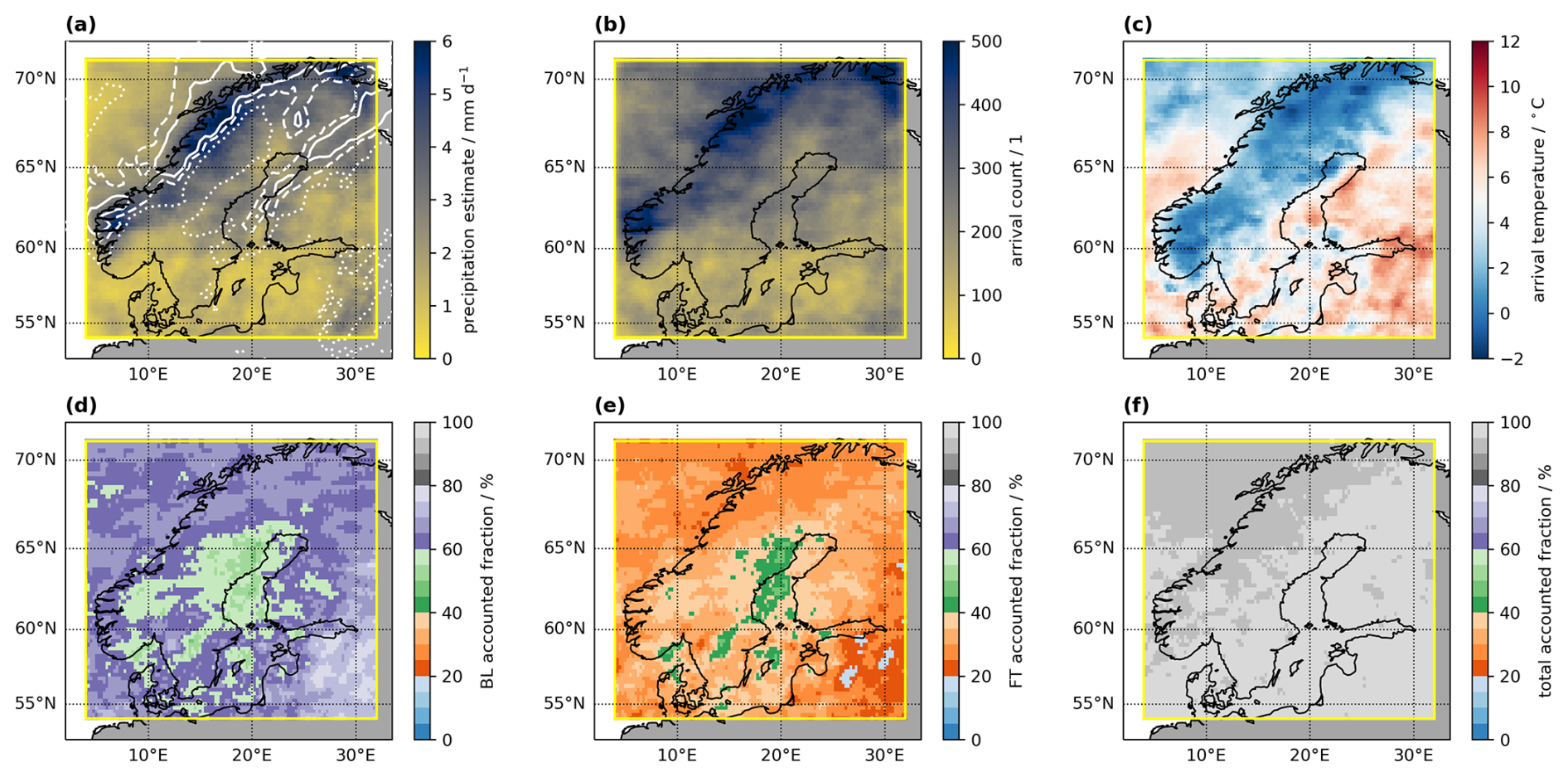
Figure 5Arrival quantities identified for the example case in 2022. (a) Lagrangian precipitation estimate (mm d−1), (b) arrival count (shading, 1), (c) arrival temperature (shading, °C), (d) accounted fraction of from boundary-layer uptakes (shading, %), (e) accounted fraction of from free-troposphere uptakes (shading, %), (f) total accounted fraction of (shading, %). Quantities in (c)–(f) are weighted averages, using the specific humidity decrease during the last time step before arrival as a weight.
5.4 Lagrangian forward projection of moisture source quantities
As WaterSip identifies the location of a moisture source, different properties of the source region can be computed, such as the average sea surface temperature, or its latitude and longitude. In particular for larger arrival regions, and for those that contain geographic or climatic gradients, the source region location and its properties may vary substantially within the arrival domain. In order to make such spatial differences in the source region properties visible, WaterSip provides Lagrangian forward projections (LFPs) of the source region properties on a spatial grid covering the arrival domain.
LFPs are obtained as the weighted average of a given moisture source property for each trajectory. The weighted average is then gridded on the arrival grid, weighted by fk. Thus, for each trajectory k, a moisture source or transport quantity ζ is transferred from the geographic uptake location (λu,ϕu) to the geographic location at the arrival region (λa,ϕa) using the fractional contributions obtained from the accounting step as a weight, and resulting in LFP quantity for air parcel k:
Hereby, U is again the number of all moisture uptake events identified along trajectory k. The different are then again gridded using Eq. (19). In creating LFPs, an important choice is whether the total accounted fraction of the precipitation estimate is used in the gridding, or only the boundary layer or free troposphere fraction. Parameter forwardProjectionMode in parameter section Diagnostics determines this choice (1: boundary layer, 2: free troposphere, 3: total fraction).
For the case study over Scandinavia, the mass-weighted moisture source latitude (centroid latitude) ranges from 50–60° N, with a clear latitudinal gradient (Fig. 6a). Corresponding moisture source longitudes range from −60 to 40° E (Fig. 6b). The source distance map for the example case shows a similar pattern as the source longitude, with more nearby sources (< 1500 km) over Denmark and southern Sweden in the southwest, and patches of more long-distant transport (> 3500 km) in the north of the domain (Fig. 6c). The distance of the moisture sources is computed as a spherical distance for each uptake location and then gridded according to Eq. (20). These examples already illustrate how forward projections of source region properties provide insight into the spatial variability within the arrival domain. When used on large (global) domains, Lagrangian forward projections can provide interesting hydro-climatic insights (Laederach and Sodemann, 2016; Sodemann, 2020).
The source land fraction (Fig. 6d) reveals a northwest-southeast oriented gradient in land uptakes. While land sources in the northwest of the domain are < 30 %, their share reaches above 80 % over the Baltic states. The fraction of land sources is obtained from evaluating a land-sea mask at the locations below the moisture uptakes. In the case where the mask file contains fractional land cover information, values above a threshold of >0.5 will classify the source location as land.
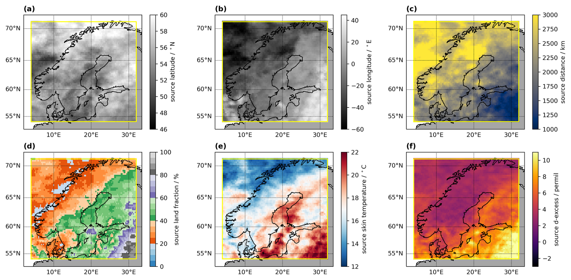
Figure 6Lagrangian forward projection of source quantities for the example case in 2022. (a) Moisture source latitude (shading, ° N), (b) moisture source longitude (shading, ° E), (c) moisture source distance (shading, km), (d) moisture source land fraction (shading, %), (e) moisture source skin temperature (shading, °C), (f) d-excess of water vapour at the moisture source following Pfahl and Sodemann (2014) (shading, ‰). All quantities are weighted averages, using the Lagrangian precipitation estimate as a weight.
The moisture source temperature is obtained here from the skin temperature (SST over ocean regions, SKT over land) using Eq. (20) (Fig. 6e). For the present case, moisture source temperatures are warmest in regions where land sources dominate with up to 22 °C. Additionally, the LFP of moisture source relative humidity, air pressure at the sources, and specific humidity at 2 m (q2 m) at the sources may be available, depending on what has been written out to the FLEXPART and LAGRANTO input files (Table D1).
Stable water isotopes are an important diagnostic in moisture source analyses (e.g., Aemisegger et al., 2014). Measurements of the secondary water isotope parameter d-excess can reflect the relative humidity environment during evaporation. In the case that SKT and q2 m or RH and T2 m are available on the input files, an approximation for the stable water isotope parameter d-excess at the moisture sources dsrc can be computed from the relation of Pfahl and Sodemann (2014):
Thereby, the relative humidity with respect to SST (RHSST) is obtained using saturation vapour pressure according to Flatau et al. (1992). For the example case, the computed dsrc shows a gradient that mirrors land properties, with higher values (8 ‰–10 ‰) where land sources dominate, while ocean source dominated regions show with ∼ 4 ‰ values below the global average in precipitation of 10 ‰ (Araguás-Araguás et al., 2000). The d-excess parameter is both an interesting diagnostic for paleoclimatic studies, and can be used to relate moisture transport to water isotope measurements on meteorological time scales (e.g., Weng et al., 2021).
5.5 Lagrangian forward projection of moisture transport quantities
In a similar way as moisture source quantities (Eq. 20), it is possible to project transport quantities onto the arrival region. The only difference is that all trajectory points, and not just the uptake points are included, using the current accounted fraction. For example, , the forward projected moisture transport temperature valid during arrival of air parcel k is obtained by averaging the air parcel quantity ξk along the entire transport path of N time steps, using the explained fraction at step as a weight:
The LFP of the moisture transport temperature obtained this way shows relatively warm transport for the majority of air masses between 6–12 °C (Fig. 7a). In comparison, the condensation temperature, computed as transport temperature conditioned on RH >80°C, shows that saturation is reached at colder and more variable temperatures of between 2–8 °C throughout the domain (Fig. 7b). Comparison to the transport pressure shows transport at higher pressures in the regions of warmer condensation temperatures, with air pressure of above 990 hPa over the Norwegian Sea, compared to ∼ 950 hPa over the Baltic Sea (Fig. 7c).
A quantity that allows to inspect the time scale of moisture transport is the transport time, obtained as the difference between the time of each uptake event and the corresponding arrival time. For the example case, the transport time shows the largest values with 5–7 d in northern Scandinavia, whereas Denmark and southern Sweden have transport times of 3 d and below (Fig. 7d). The transport time in this case thus bears similarities with the transport distance (Fig. 7e) and the direct source distance map (Fig. 6c). In contrast to the moisture source distance, the transport distance is obtained as the total distance along an air parcel trajectory. The difference plot between both distance quantities underlines that the transport distance is always larger than the source distance, and more so for regions where transport takes more time, with a differences of up to 2000 km in Northern Scandinavia (Fig. 7f). In combination, these transport quantities enable one to interpret the transported moisture in terms of processes that occurred underway from source to sink. Such information can for example be relevant for understanding changes of isotope composition and the mixing with other air masses. For more detailed discussion of the transport time from WaterSip, see Sodemann (2020) and Gimeno et al. (2021).
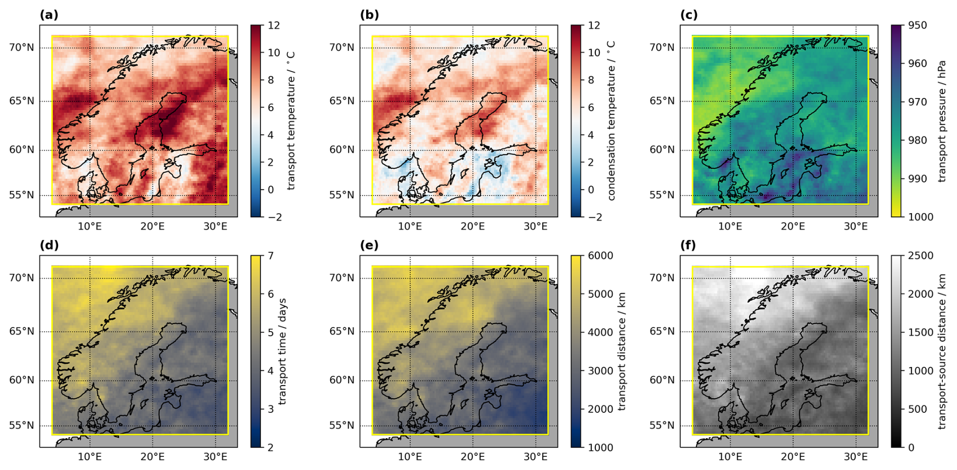
Figure 7Lagrangian forward projection of transport quantities for the example case in 2022. (a) transport temperature (shading, °C), (b) condensation temperature (shading, °C), (c) transport pressure (shading, hPa), (d) transport time (shading, days), (e) transport distance (km), and (f) difference between transport and source distance (km). All quantities are weighted averages, using the Lagrangian precipitation estimate as a weight.
5.6 Time series of diagnostic quantities
The temporal evolution of different diagnostic quantities in the arrival domain can provide further insight into moisture transport dynamics. WaterSip provides time series output of all arrival and forward-projected source (ζ) and transport quantities (ξ) described above (Sect. 5.3–5.5). Thereby, the mean, median, and the maximum and minimum value are reported for different integration times, from the trajectory time step to daily, monthly, yearly, and the entire analysis time period (Table 2). Longitude is thereby converted to a Cartesian grid for the averaging operation. Averaging over time steps is done by weighting the contribution at each time step i of the analysis period with the corresponding precipitation estimate at grid location (λa,ϕa), and dividing by the total of the precipitation estimate for a given averaging period T:
Time series of of the case study obtained this way show a pronounced precipitation maximum in the first half of the study period on 5 to 7 August 2022 with 1.0 mm (6 h)−1 (Fig. 8a, black solid line). A second maximum occurred with about 0.8 mm (6 h)−1 on 10 August 2022. The ERA5 precipitation shows that WaterSip underestimates domain average precipitation during these periods, but not during weaker rainfall events (Fig. 8a, blue line). The standard deviation of the precipitation estimate in the arrival domain reflects some of the peak values present in ERA5 (dashed line).
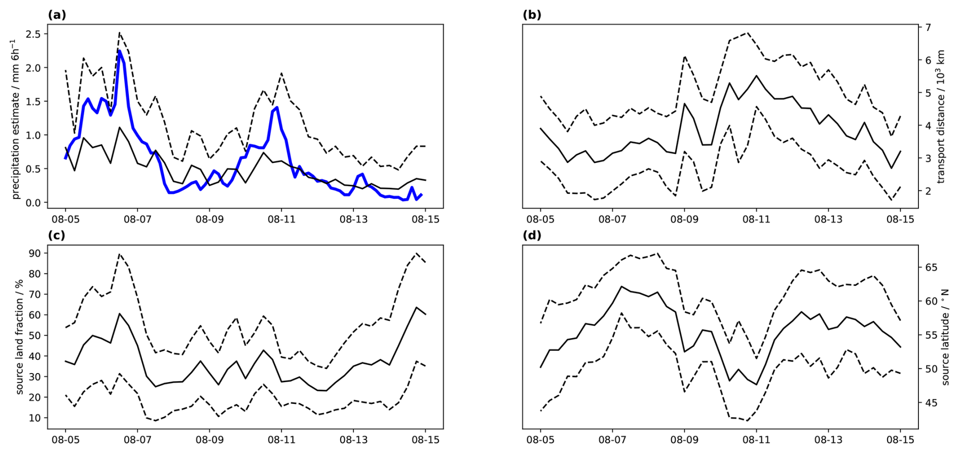
Figure 8Time series output from WaterSip for the Scandinavian precipitation from 5–15 August 2022 for the variables (a) precipitation estimate (mm (6 h)−1, black line) and ERA5 simulated precipitation (thick blue line), (b) transport distance (103 km), (c) source land fraction (%), (d) source latitude (° N). Each panel shows the weighted mean (solid line) and unweighted 1σ standard deviation (dashed lines) over the arrival grid.
The period with most intense precipitation was associated with gradually shorter transport distances of less than 3000 km (Fig. 8b). Land sources were dominating in the first period, with a fraction up to 60 % on 6 August 2022, compared to below 30 % on 12 August 2022 (Fig. 8c). Source latitudes were more northerly during the first half of the case study, and dropped to below 50° N on 10 August 2022 (Fig. 8d). Both characteristics match well with the moisture source snapshot for that day (Fig. 3a).
During the forward projection, some grid points have only a very small number of trajectories arriving, which can then lead to relatively large grid maximum and minimum values compared to the overall spread. For some applications, a more refined statistical quantification of the gridded fields may be required, for example such as excluding grid locations below a minimal precipitation estimate. In such a case, users may choose to output the gridded fields for every time step, and then follow up with their own post-processing steps.
5.7 Sectorisation of source region maps
Another post-processing available within WaterSip is the option to categorise the moisture source maps by geographic domains, the so-called sectorisation (Sodemann and Zubler, 2010). During sectorisation, the coordinates of each uptake in the boundary layer and free troposphere are checked to be within a set of J latitude and longitude bounds [λj,ϕj], which define the source sectors Sj. The geographic bounds of each sector are implemented in the program code as a function that returns the sector number corresponding to a given geographic coordinate. Currently, 11 different sectorisations are available in WaterSip (Table C1). Implementing additional sectors requires users to modify the WaterSip code. Further details are given in the Appendix C.
The output from the sectorisation is included in the time series files (Table D3). All quantities available on the source and transport grids contain an additional dimension for the sector number. Furthermore, quantities are given for land regions only, sea only, and for the total. This allows to define relatively simple geographic sector shapes that still make the important distinction between land and ocean regions, based on the land-surface information provided to WaterSip. The sector areas are also available to convert the fractional output to mass units.
For the case study over Scandinavia, the sectorisation “Norway” has been chosen, which includes 8 latitude sectors (Fig. 9c). The total arriving precipitation is dominated by sources at 50–60° N (Fig. 9a, light green) in the first half of the study period, before being dominated by more southerly sources in the second half (40–50° N, dark green). Splitting up the moisture originating from land areas only further emphasises that the shift to more northerly sources is driven by land contributions from 30–40° N (Fig. 9c). In a tabular summary, it becomes evident that ocean sources still dominate for the entire event period, and that less than 10 % of the precipitation originate from south of 40° N (Table 3).
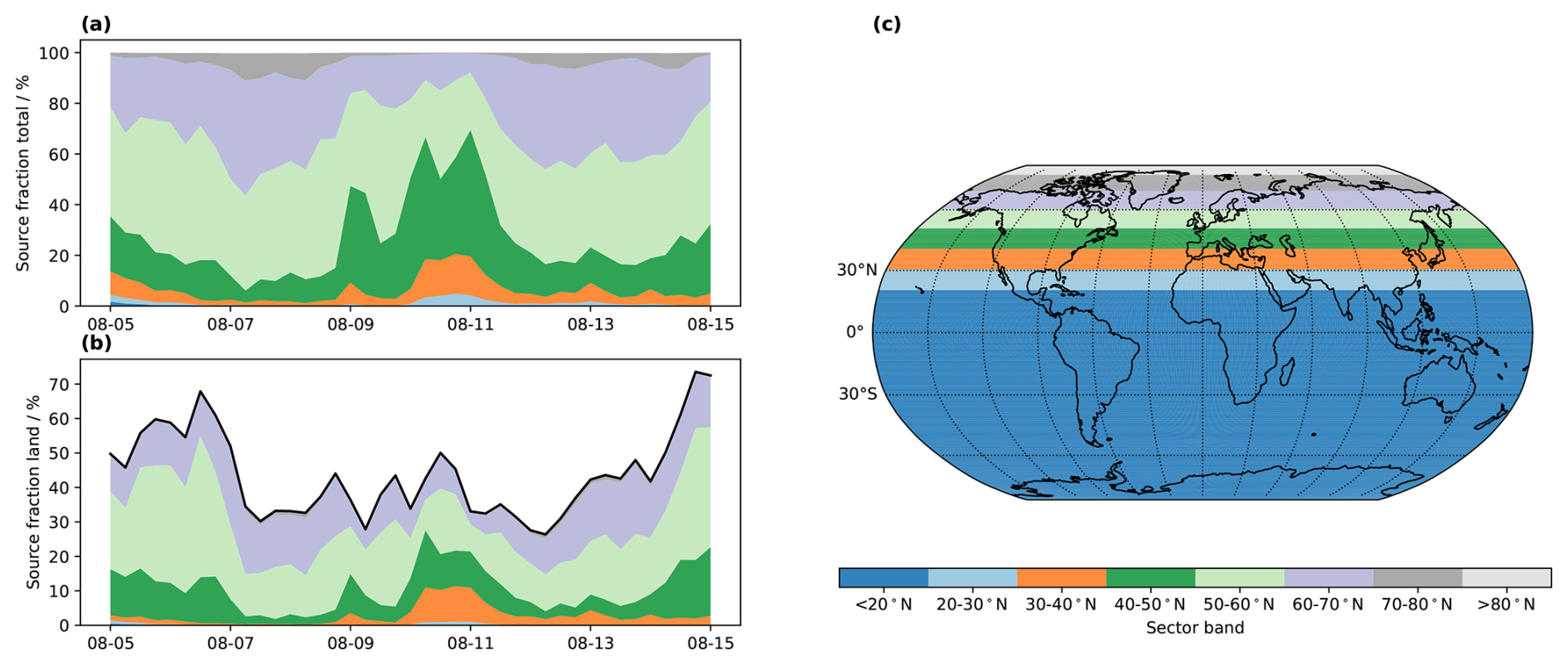
Figure 9Sectorisation example for the Scandinavian case study for August 2022. (a) Classification of the total (land and ocean) moisture sources into latitude bands between 20–80° N during the study period. (b) Classification of the land sources only. Solid black line indicates the total fraction of all land sources. (c) Sector map of sectorisation “Norway” (#3) used in the case study.
Table 3Sectorisation results in percent separated into boundary layer and free-troposphere moisture sources for the total, and over land and sea regions only, for the Scandinavian case study for August 2022.
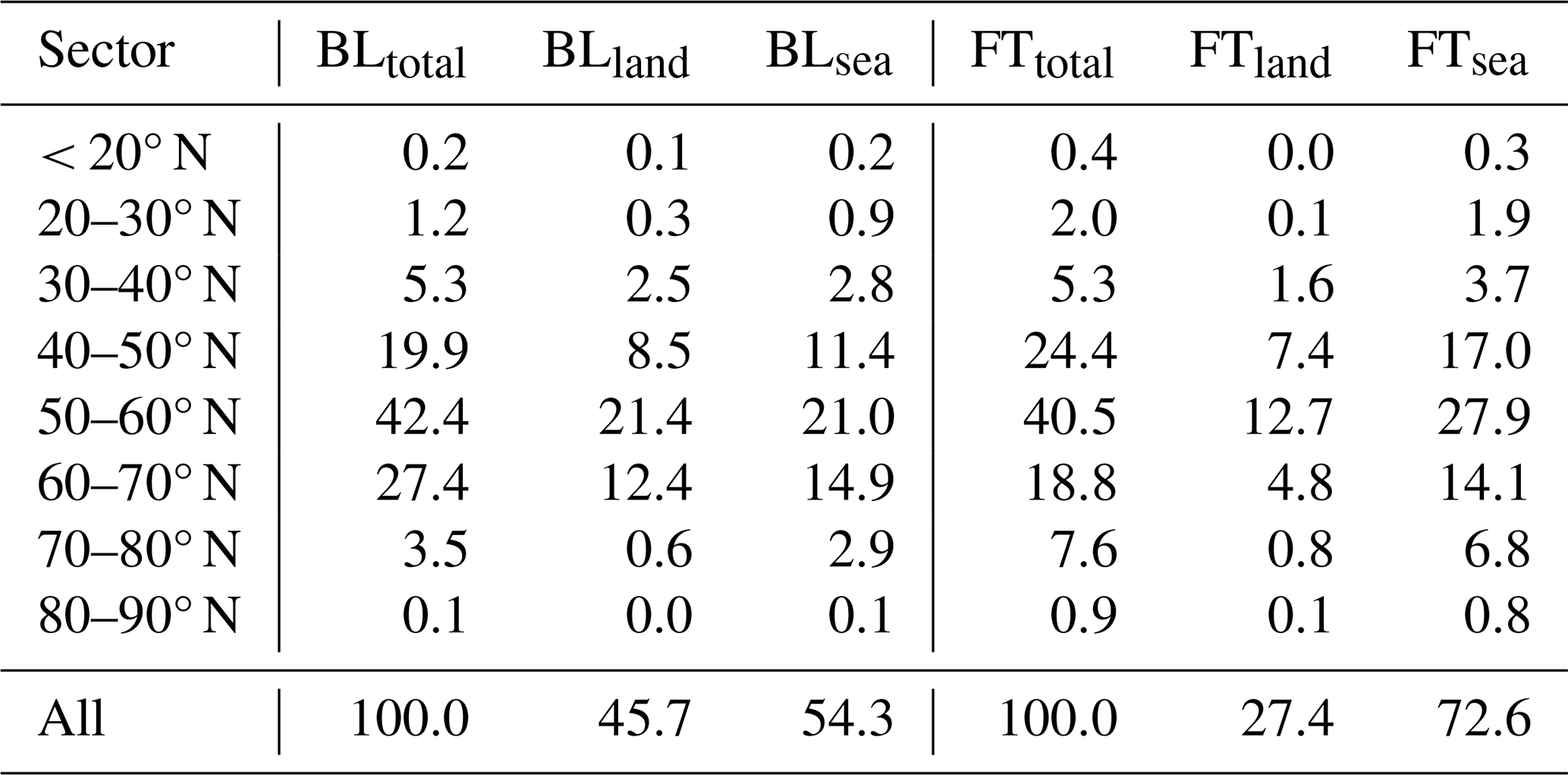
5.8 Histograms of moisture source and transport properties
For some applications, it may be valuable to have the source and transport information from WaterSip available from every single uptake event. During the gridding to source or arrival grids, this detail of information is lost. Since the number of individual uptakes can be very large, histograms are a convenient way to aggregate such data. For example, Winschall et al. (2014b) used histograms of transport time to identify the age spectrum of precipitation. Other examples for the use of such output are the distribution of SSTs at the moisture sources (Weng et al., 2021). WaterSip creates an output file in comma separated value (csv) format containing histograms of a fixed set of variables as output if the parameter saveHistogram in setting group Output is set to 1 (true). These variables include convection count and depth, uptakes, rainout, air mass mixing, source SST or T2m, source distance, source d-excess, and RHSST at the sources (Table 4). As the histogram classification is implemented directly within WaterSip, changes to the classification parameters, or adding more variables requires changes to the WaterSip program code in file Water.cpp.
For the example case of Scandinavia during August 2022, the probability density function of the uptake contributions shows a maximum at 2 d before arrival, and a rapidly decreasing tail thereafter to 10 d before arrival (Fig. 10a). The distribution of rainout events (not weighted by f) also peaks at 2 d before arrival time, but has otherwise an even distribution throughout the 20 d analysis period (Fig. 10b). The PDF of mixing events (also not weighted by f) peaks at 4 and 8 d before arrival (Fig. 10c). Finally, the PDF of source distances shows a rapidly flattening tail with the majority of sources within about 5000 km (Fig. 10d). These examples illustrate the additional insight that one can gain from the histogram data, beyond the mass-weighted averages provided by the gridded and time series output.
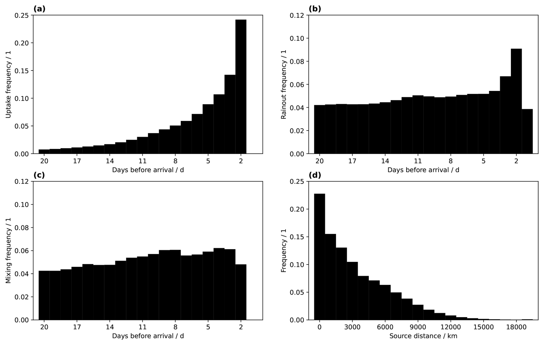
Figure 10Histograms of moisture source and transport quantities for the example case. (a) frequency of uptake events by time before arrival, (b) frequency of rainout events by time before arrival, (c) frequency of mixing events by time before arrival, and (d) frequency of uptakes by source distance. All histograms are valid for the entire analysis period and have been converted to probability density functions. The weighting for each quantity is listed in Table 4.
Table 4Histogram variables currently built into WaterSip, with corresponding lower and upper bounds, and number of categories for the classification.
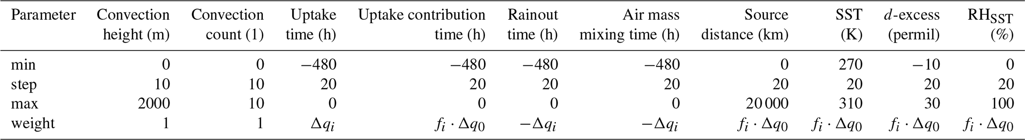
5.9 Air parcel trajectory output
WaterSip processes air parcel trajectory data obtained from the Lagrangian models LAGRANTO and FLEXPART. During the processing of these data, trajectories are filtered based on criteria such as being located within the arrival domain, precipitating during arrival, and so on. Essentially, thus, the WaterSip tool creates a subset of the original trajectory data, enhanced by additional information, such as the identified uptakes, and the accounted fraction. Setting parameter saveTraj of settings group Output to either 1 (output every time step) or 2 (output in monthly files) instructs WaterSip to write out these trajectory data in a compact binary format (*.traj). Since the total output size can become rather large, it is possible to use parameter skipTraj with a value n>1 to only write out trajectories for every nth particle. A python script for reading the binary format is provided in the WaterSip code repository.
The potential value of the trajectory output is illustrated here for a subset of the air masses arriving over the target area in Scandinavia at 06:00 UTC on 10 August 2022. During this time, 20 d backward trajectories tap into moist air masses in the Gulf of Mexico and the subtropical North Atlantic, and to a lesser extent into the Pacific basin (Fig. 11a). The colour shading by moisture uptakes and losses emphasises regions of moisture gain over the eastern and western North Pacific (blue), over North America, and the North Atlantic, as well as moisture loss as air parcels approach Scandinavia (red). The time vs. height diagram illustrates that in this case much of the moisture gained more than 10 d before arrival has been lost due to the vertical lifting and drying of air masses at about −10 d (Fig. 11b). Another branch of air descended from the upper troposphere between 6–10 km (dark brown colours) before taking up moisture in the lower troposphere. In some cases, the remaining moisture may also have been been overwritten by uptake events during the last 10 d before arrival, as exemplified by the trajectory highlighted in red that rises and then sinks again towards the surface multiple times.
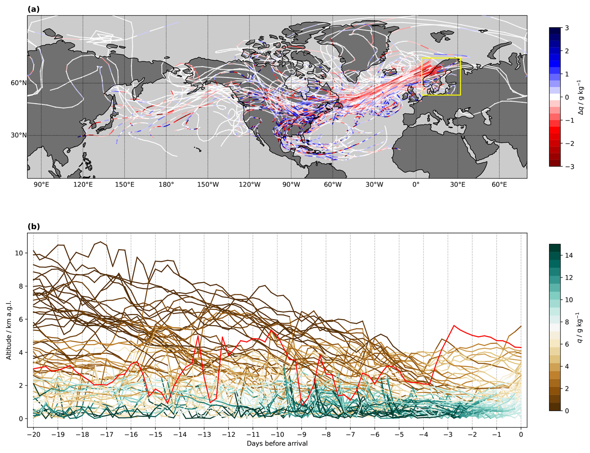
Figure 11Trajectory output from WaterSip for 06:00 UTC on 10 August 2022. (a) Map of the moisture transport pathway of 20 d trajectories shaded by specific humidity changes per time step (Δq in g kg−1 6 h−1). (b) Time vs. height diagram shaded by specific humidity (g kg−1) for water vapour arriving in the Scandinavia domain. For illustrative purposes, a random selection of 70 out of 8000 air parcel trajectories is displayed. The trajectory highlighted in red illustrates the repeated vertical movement of some particles on the way to the target region.
As mentioned throughout the description of the method, there are a number of uncertainties connected to the use of the WaterSip diagnostic. A sensitivity study for the Scandinavia case illustrates how WaterSip responds to variations in key parameters (Sect. 6.1). Users need to carefully consider the impact such uncertainties may have on the interpretation and validity of their results (Sect. 6.2). Underlying this uncertainty is the lack of a direct observable quantity that would serve as a reference for finding out moisture source information. In that context, method inter-comparisons and sensitivity studies can be a pathway to quantify and potentially bound uncertainty (Sect. 6.3). Lastly, some computational performance characteristics of the software are presented (Sect. 6.4).
6.1 Sensitivity analysis of key parameters
Using the Scandinavia case study discussed above, a range of sensitivity experiments was conducted to illustrate the sensitivity of the diagnostic to several core parameters. The domain averages of the precipitation estimate , total accounted fraction ftot, and the source distance have been chosen as bulk properties of the moisture sources during the event. When the critical relative humidity RHc was varied from the reference value 80 % to 70 % and 90 %, increased or decreased about 25% compared to the reference value of 2.074 ± 1.162 kg m−2 (Table 5). This can be expected due to more (less) precipitation events being detected at arrival for a lower (higher) RHc. In comparison to the domain-average ERA5-simulated precipitation of 2.43 kg m−2 d−1, the underestimation amounts to 17 % for the reference case. The moisture source distance increases slightly with a higher RHc, while ftot remains nearly unchanged.
Table 5Sensitivity experiments with key parameters using the Scandinavia case study from August 2022 as a reference. Source characteristics are given in terms of domain averages of precipitation estimate , total accounted fraction ftot, and source distance. The reference experiment uses RHc=80 %, Δqc=0.2 g kg−1, Len = 81, and Tstep = 6 h. Differences are computed as Experiment – Reference. For details see text.
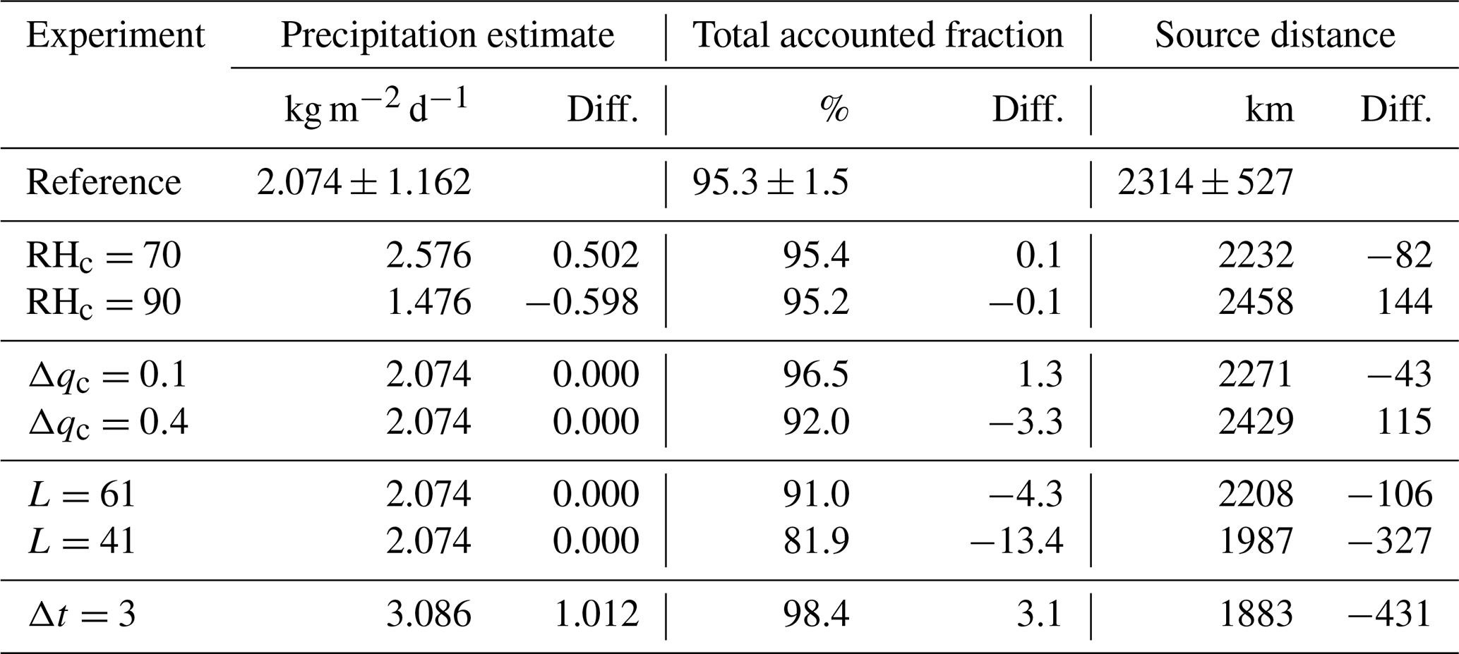
Sensitivity with regard to the value of Δqc was tested with 0.1 and 0.4 g kg−1 6 h−1. The precipitation estimate remained unaffected by this change, since the humidity change during the last time step is set by the separate parameter arrivalPrecipThreshold. The total accounted fraction decreases with increasing Δqc, since less events are identified as moisture uptakes. A higher Δqc also favours slightly more distant moisture sources, as less discounting of remote moisture takes place for the case study.
The trajectory length has a clear imprint on ftot, with 13.4 % less accounted sources for 10 d (L=41) compared to 20 d (L=81) trajectories. In comparison, the difference between 15 and 20 d trajectories is only 4.3 %. The moisture source distance is also sensitive to the trajectory length, with on average 327 km closer moisture sources for the 10 d trajectories. Still, the average value is less than the 1σ standard deviation within the domain of 527 km, and remains within 15 % of the reference value for all of the above parameter variations.
Finally, the sensitivity to the time step Δt has been tested using a 3 h time interval. To enable a fair comparison to the reference, this run also required adjustment of Δqc to 0.1 g kg−1 3 h−1, and increase of the trajectory length to 161 time steps to maintain 20 d trajectories. The results for this sensitivity test deviate more markedly from the reference than the previous sensitivity experiments, with a 50 % higher precipitation estimate, a 3.1 % higher ftot, and a 431 km closer source distance than the reference. This kind of response in the results of the diagnostic can be explained by the increasingly ambiguous distinction between variations in specific humidity from moisture uptakes that the diagnostic aims to identify, and variations from interpolation errors and other random factors. Users should carefully evaluate which time step and specific humidity thresholds are suitable for their study.
6.2 Error sources and uncertainties
As other Lagrangian moisture source diagnostics, WaterSip calculates the Lagrangian water budget of air parcels that are moving with the atmospheric flow. At initial time t0, these air parcels are defined by their location, an assumed spatial extent, and represent an atmospheric mass mk. As air parcels move horizontally and vertically, their shape is assumed to be maintained, as well as the total mass. However, exchange processes across the air parcel's imaginary walls can modify the amount of water vapour within the air parcel, as quantified by the specific humidity q (g kg−1). Interpolation errors can then, among others, cause spurious variations in the specific humidity. Another assumption that is made in the Sodemann et al. (2008b) algorithm is that during one time step, all specific humidity changes are assumed to either be due to uptakes or losses, while in fact it is a net change that may include both uptakes and losses in the time interval. While this assumption is more valid the shorter the time interval between trajectory points, shorter time intervals also lead to using smaller Δqc between time steps, which then becomes more difficult to separate from interpolation noise. Another assumption in WaterSip is that diagnosed evaporation took place at the geographic location where the moisture uptake has been detected. However, this does not necessarily need to be the case, for example when water vapour that had evaporated earlier is at a later time mixed into an air parcel as a result of mixing from turbulence or convection.
While threshold parameters, such as Δqc are used to suppress some of the numerical noise introduced during the trajectory calculation and interpolation, there may either be too many uptakes diagnosed, or some uptake events may be missed. The total explained fraction ftot can then provide important guidance whether the accounting works consistently (i.e., ftot≤1) with the chosen threshold parameters. Spurious variations that are larger than the threshold value will lead to more remote moisture being discounted in the favour of later uptakes, while the assumption that either evaporation or precipitation take place during one time step acts to overestimate remote sources. Such potential biases are important to keep in mind during interpretation.
Other important sources of uncertainty are the number of particles chosen to represent the investigated air mass, as well as the time step of the trajectory output. In general, a larger number of trajectories will provide better statistical representation of the diagnosed quantities, in particular when used with a particle dispersion model such as FLEXPART that parameterises turbulent and convective motions. The number of particles should also be chosen in line with the resolution of the source and arrival grids, providing reasonably smooth and continuous gridded output. Other considerations of offline trajectory diagnostics are the effects of data assimilation, which provides humidity increments during the process (Fremme et al., 2023), and from parameterisation schemes in the parent numerical model. Here in particular the role of convection schemes is important to consider, providing both a pathway for rapid specific humidity changes and vertical particle motion that are hard to capture in offline calculations, even when using parameterisation schemes for convection in the trajectory model (Sodemann, 2020). Here, the use of online trajectory calculation methods (Miltenberger et al., 2013) could provide a pathway towards quantifying such uncertainty.
Table 6Overview over computational time and memory demand when running the WaterSip diagnostic for the Scandinavia test case and a test case covering a larger domain (0–90° N and 90° W–90° E). Sensitivity experiments with different number of particles and different cores illustrate performance characteristics. All runs were performed on a Linux machine running on a 36-core Intel(R) Xeon(R) Gold 6140 CPU at 2.30 GHz.
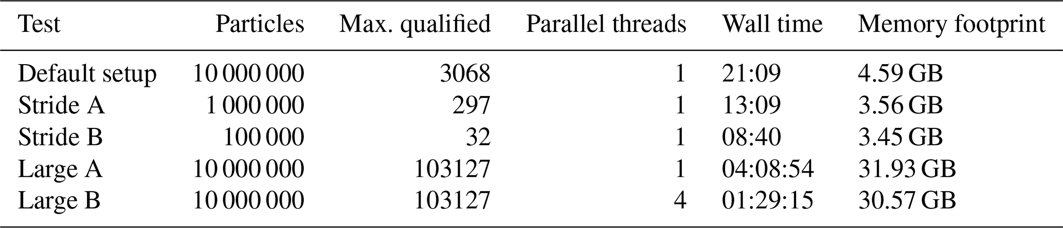
6.3 Quantifying and reducing uncertainty
Future development of the WaterSip software and similar approaches will benefit from quantifying uncertainty, and from identifying the contribution of different factors to uncertainty. In the absence of a direct observable quantity for the water vapour origin, model inter-comparison efforts are important. First steps in this direction have been made by van der Ent et al. (2013) who employed a regional tagged water tracer simulation as the reference standard for a Eulerian moisture source identification algorithm. Similarly, Winschall et al. (2014a) and Laederach (2016) compared the WaterSip diagnostic to tagged tracer simulations from a regional model. While tagged tracers do have limitations with regard to the representation of different processes in the atmospheric water cycle at small scales, it can be expected that using such online simulations as input data for offline diagnostics can help to quantify uncertainty, essentially serving as an internal “gold standard” for such inter-comparison efforts (Sodemann, 2020). Thanks to the availability of an increasing number of approaches to provide (Lagrangian and Eulerian) offline moisture source diagnostics as open access software (van der Ent et al., 2014; Keune et al., 2022; Fernández-Alvarez et al., 2022), the feasibility of such an inter-comparison effort has greatly increased in recent years. The present description of the WaterSip diagnostic is another piece in the puzzle that may help to advance ongoing debates. On the longer run, the availability of suitable water vapour isotope measurement data sets, in particular such that connect moisture source signals with measurements along the transport pathway and the arrival region, have the potential to indeed constrain diagnostic methods by measurements (Gimeno et al., 2021).
6.4 Computational performance characteristics
The test case here is run only for a short time period and over a spatially limited domain. Running on a single core on a 36-core Intel(R) Xeon(R) Gold 6140 CPU at 2.30 GHz, the diagnostic completes after about 21 min, with a peak memory use of 4.6 GB (Table 6). Important aspects of the duration of the computational time are the amount of input/output (I/O) operations, and the number of particle trajectories to be processed. The test case has at most about 3000 new particles that are qualified for tracking within each time step of the test case period. This means that here I/O dominates over the amount of time spent for evaluating the moisture source changes and gridding the results. When the amount of particles considered for analysis is reduced by a factor of 10 (Test “Stride A”) or 100 (Test “Stride B”), the computation time only decreases by a factor of 0.4 or 0.6, respectively. Nonetheless, a stride larger than one provides results substantially faster, which is useful for example when testing an analysis setup. Note that results will however contain more gaps with fewer particles due to the stride setting. The memory footprint scales less than the computational time, since this demand is dominated by the output grids and thus the length of the analysis period. Finally, the parallelisation performance is illustrated with a run over the same time period, but with a larger domain covering half the Northern Hemisphere. The use of 4 cores (Test “Large B”) shows a 2.75× speedup compared to the single-core run (Test “Large A”). However, performance gains quickly become lower with additional cores due to the need for processes to wait for one another (not shown). It may be possible to gain faster computation times and better scaling if the code were further optimised for parallelisation.
The WaterSip software is a versatile implementation of the Lagrangian moisture source and transport diagnostic of Sodemann et al. (2008b). Besides providing a detailed, formal description of the diagnostic algorithm and its key parameters, this manuscript provides practical information to set up and run the WaterSip tool, and serves as a reference describing the format and contents of the different output files from the diagnostic. Using an exemplary case study for a precipitation period over Scandinavia in August 2022, guidance on the use and interpretation of different maps and output products from the software is provided. Using the available setup with the same input data as the case study (Sodemann, 2025a), users can get quickly accustomed with the wide range of configuration options of the software tool, and the varieties of diagnostic output, before setting up their own cases.
As other off-line diagnostics, WaterSip and its accounting algorithm have several underlying assumptions. When interpreting results from WaterSip, users are therefore advised to carefully consider all sources of uncertainty. Uncertainty arises from the choice of different parameters in the set-up of the input data in the form of air parcel transport trajectories, but also with regard to several parameters that influence the sensitivity and performance of the method. In order to obtain physically meaningful results, threshold parameters may need to be set to different values depending on the geographic region, the season, and the height in the atmosphere that is considered during an analysis. Users are therefore advised to carefully test their particular set-up in order to determine the sensitivity of their results to the chosen parameter configurations.
Availability of the software tool enables a wider use of this diagnostic for studies of the moisture source location and properties, as well as for identifying the conditions during atmospheric transport, and during arrival at the target region. Making the software code available in a public repository removes the requirement for other researchers to re-implement the diagnostic algorithm, and enables future contributions from the community such as reading output from other Lagrangian particle and trajectory models.
It is the hope of the author that documenting and making the code of WaterSip available here will lead to the further application of the tool in a wide range of regions and scientific applications, from understanding the factors of precipitation extremes, to climatological studies, and paleoclimate studies. Furthermore, WaterSip in its current version 3.2 may be compared to the results of other available moisture source diagnostics, helping to understand the overall state of the art in this scientific branch, thereby contributing to progress in the field and future methods with reduced uncertainty.
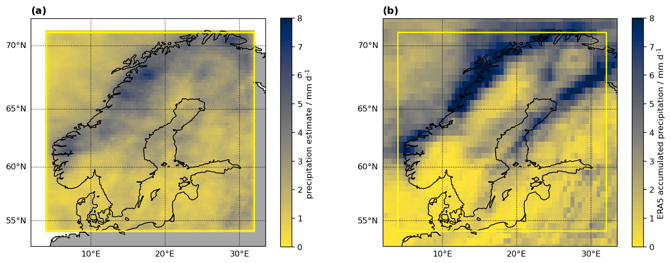
Figure A1Comparison between precipitation during the case study period (06:00 UTC on 5 July to 00:00 UTC on 15 July 2022) over Scandinavia (a) estimated from the WaterSip diagnostic and (b) from ERA5 in mm d−1.
The Lagrangian precipitation estimate for the period from 06:00 UTC on 5 July 2022 to 00:00 UTC on 15 July 2022 over Scandinavia shows a pattern that roughly follows the topography along the west coast of Norway (Fig. A1a). In contrast, southern Scandinavia and the Baltic Sea have lower total precipitation averages of 0–1 mm d−1. The ERA5-simulated precipitation has a much stronger contrast between coastal regions and the drier interior of the domain. The period average reaches above 8 mm d−1 in Northern Norway, but has also a larger extent of regions where no precipitation was predicted.
The WaterSip configuration file contains all control parameters of the WaterSip diagnostic in one text file. The control parameters are each specified on one line in the format . Parameters can be either a string, integer, boolean, or float value. Parameters are grouped into one of 7 settings groups. Corresponding tables referred to in the Appendix provide an overview over all parameters in this group, including example values.
-
Case. The settings in this group concern the basic settings of a diagnostic run (Table B1).
-
Grids. The parameters in this category specify the different output grids and the gridding method (Table B2).
-
Diagnostics. The parameters in this category control the way how the diagnostic works, and which trajectories should be considered in the run (Table B3).
-
Output. The parameters in this category determine which output files should be created (Table B4).
-
Variables. The parameters in this category allow to include or exclude specific variables from the output files. Setting the output for unused variables to 0 (disabled) will speed up computation time, reduce the memory footprint, and reduce the output file size (Table B5).
-
FLEXPART. The parameters in this category describe the properties specific to FLEXPART input files (Table B6).
-
LAGRANTO. The parameters in this category describe the properties specific to LAGRANTO input files (Table B7).
Settings groups are identified in the configuration file by their name included within in square brackets (e.g. [Case]). The 7 settings groups and control parameters within them can appear in random order in the input file. WaterSip will display an error message if a parameter name is unknown or in the wrong settings group. An error message will also be displayed if the parameter value is of wrong type. Space characters and empty lines will be ignored in the input file and can be used to format the content. In addition, comments can be added after the character “#” anywhere in the file to facilitate documentation.
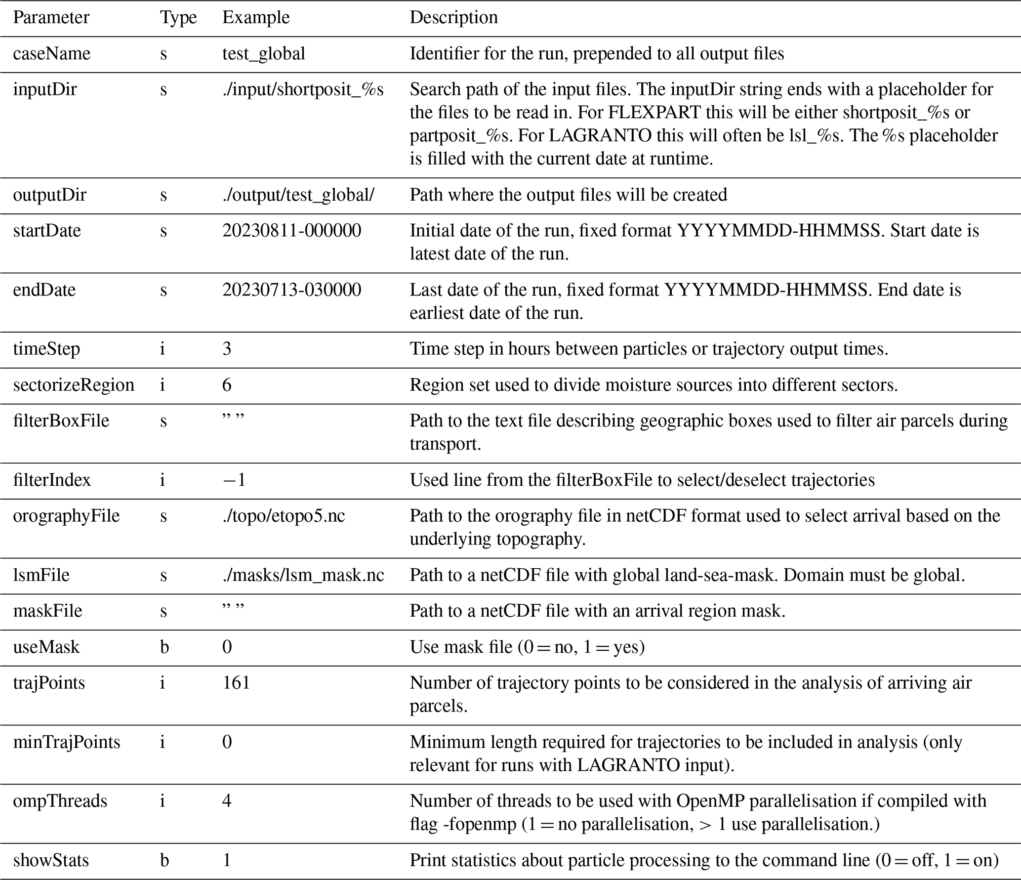
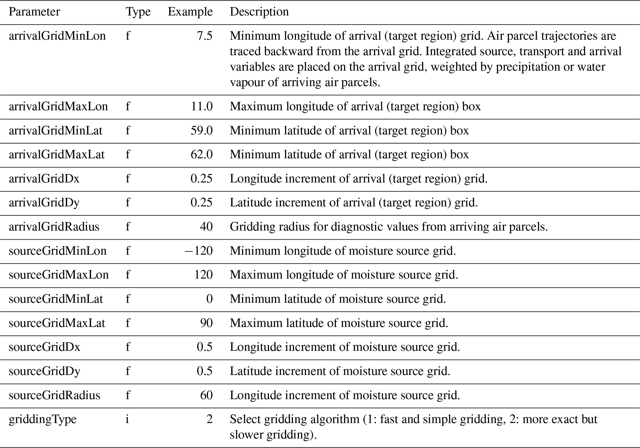
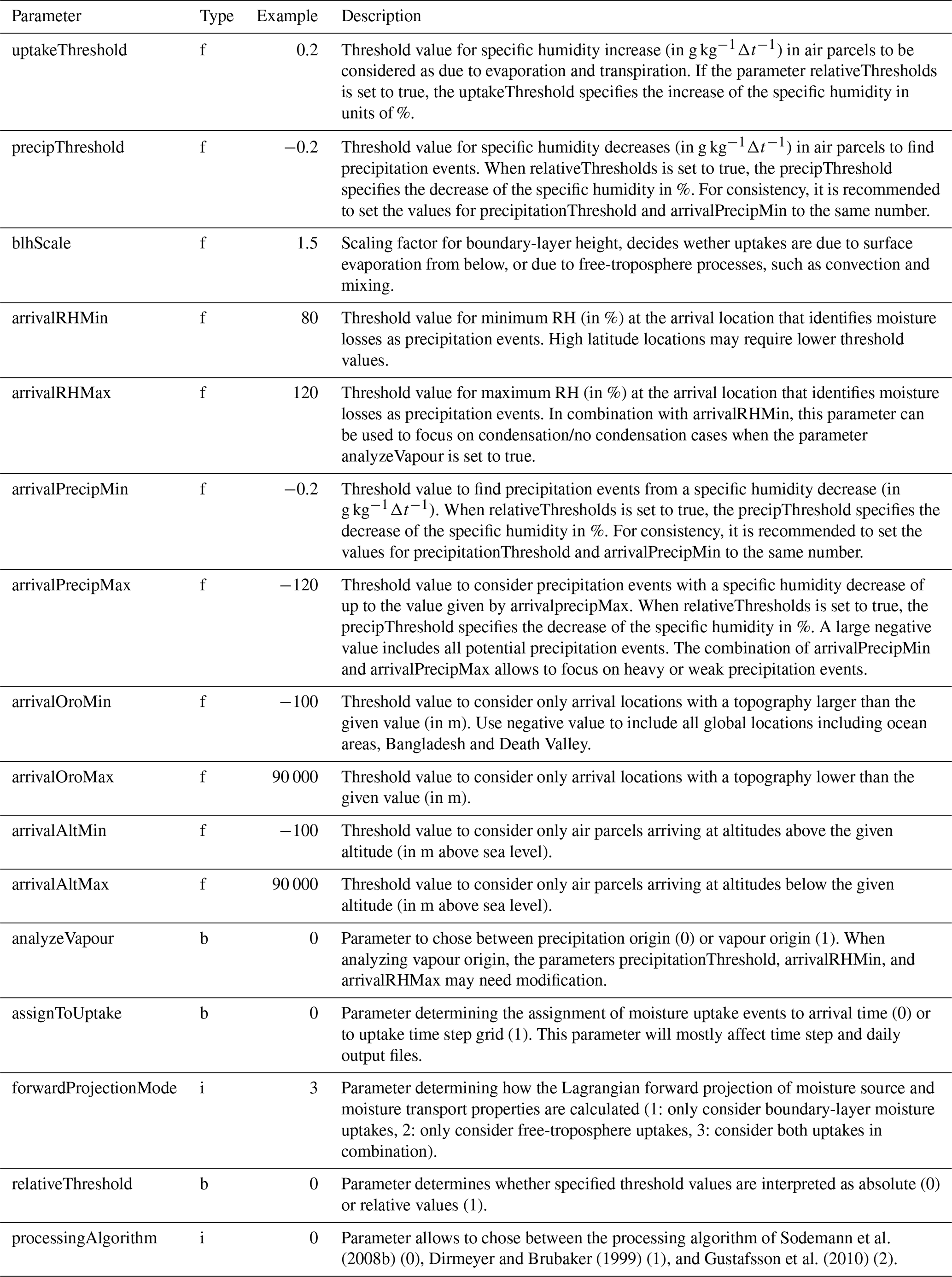
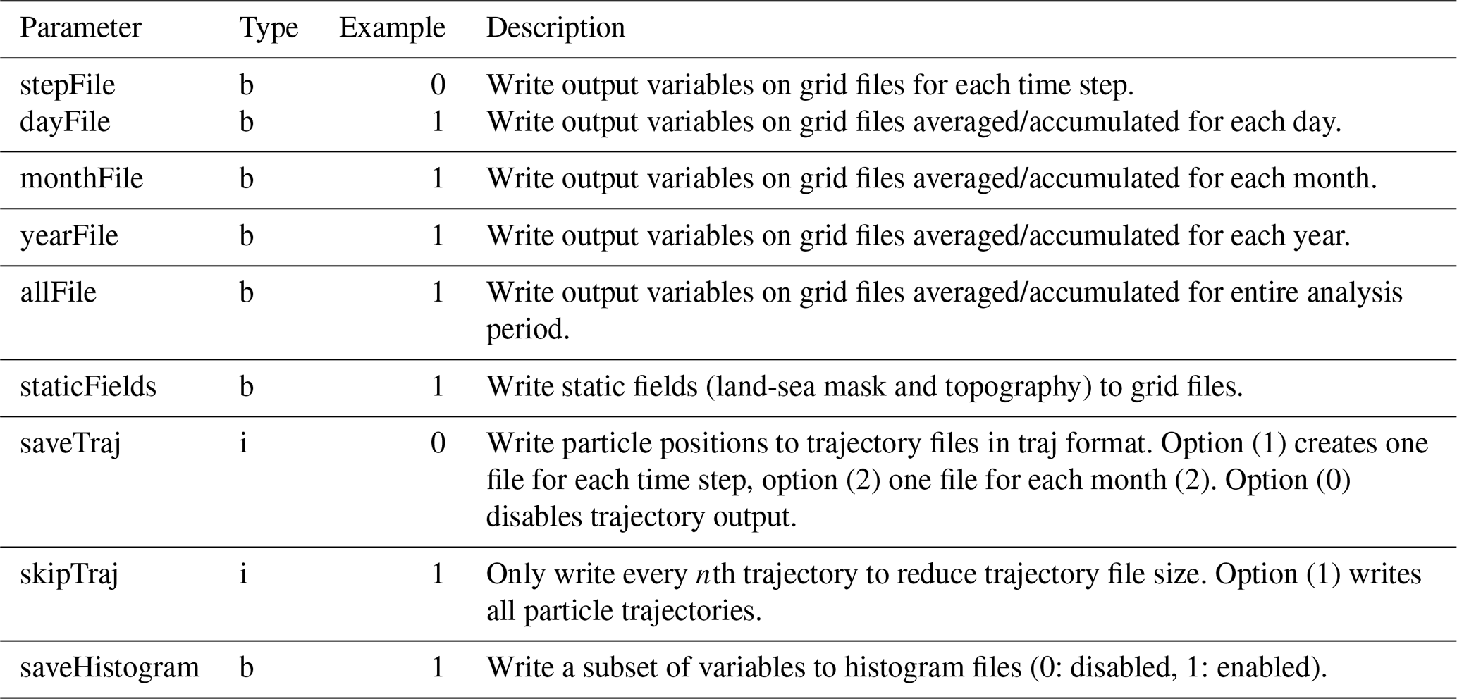
Table B5Parameters in the settings group Variables. Output of variables activated by parameter value (1) and deactivated by (0). Variables are written to grid and series output files.
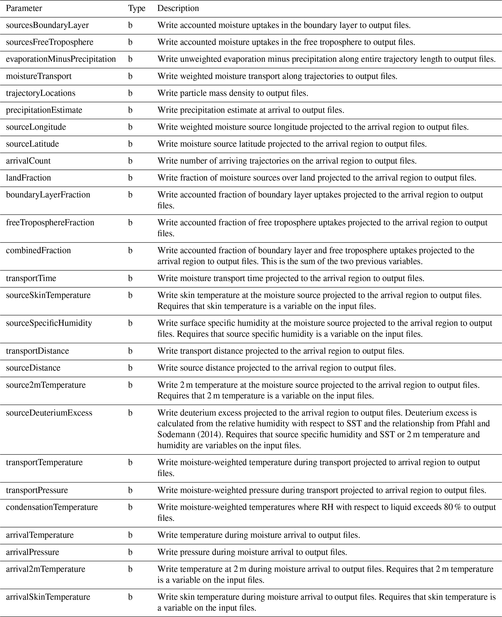
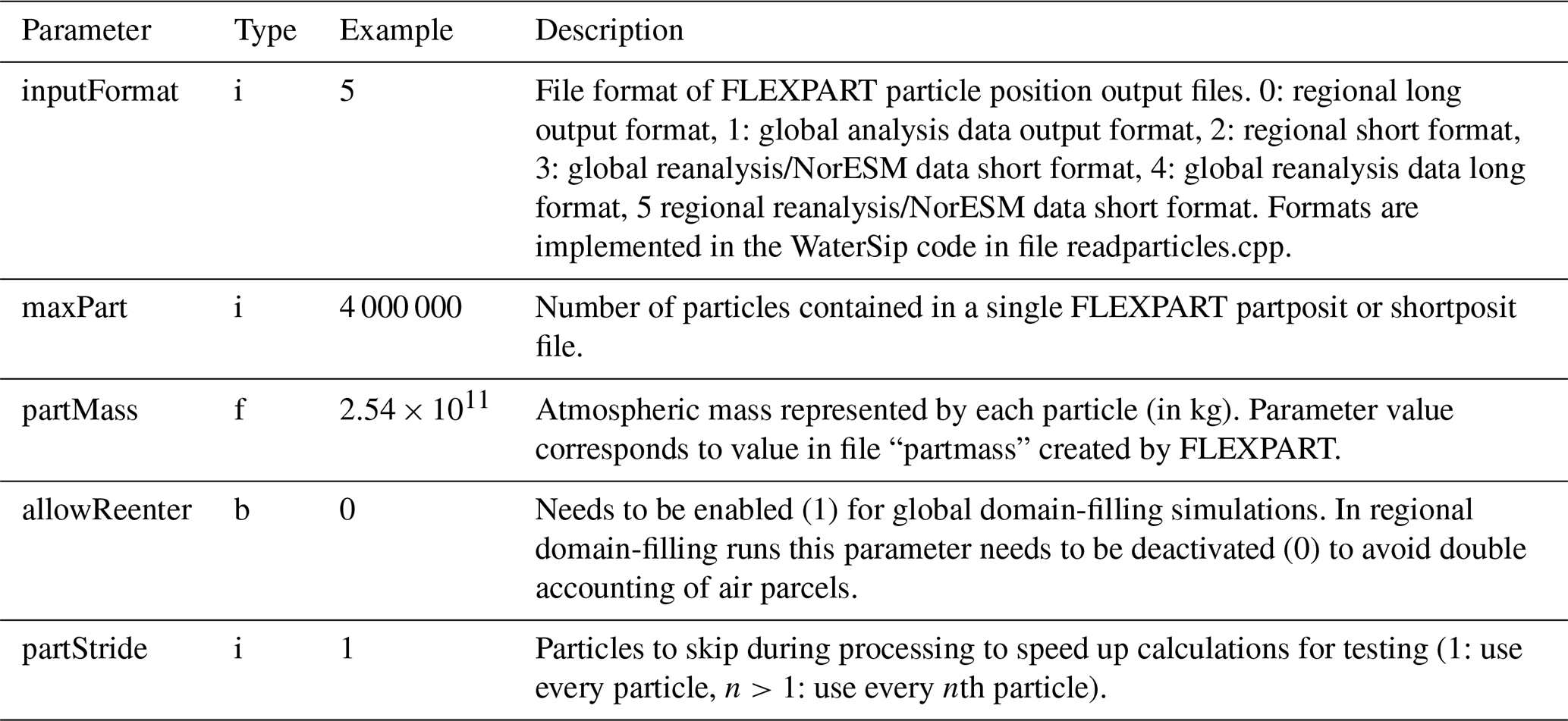
Table B7Parameters in the settings groups LAGRANTO. Variables are identified by column index, starting from 0. Variables not contained in trajectory files are specified as value −1.
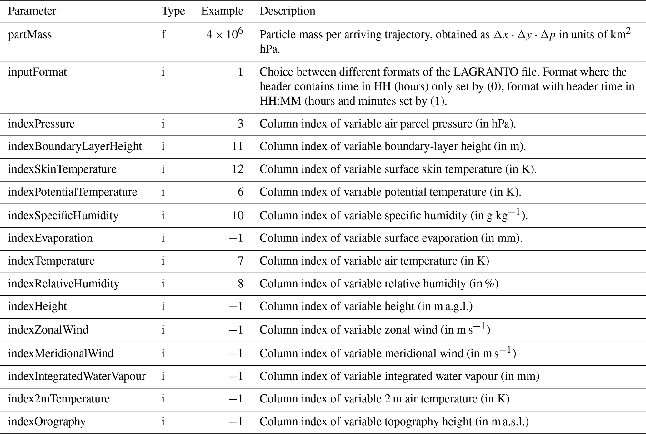
Table C1Sectorisations that are currently available in WaterSip by setting parameter sectorizeRegion in settings group Case.
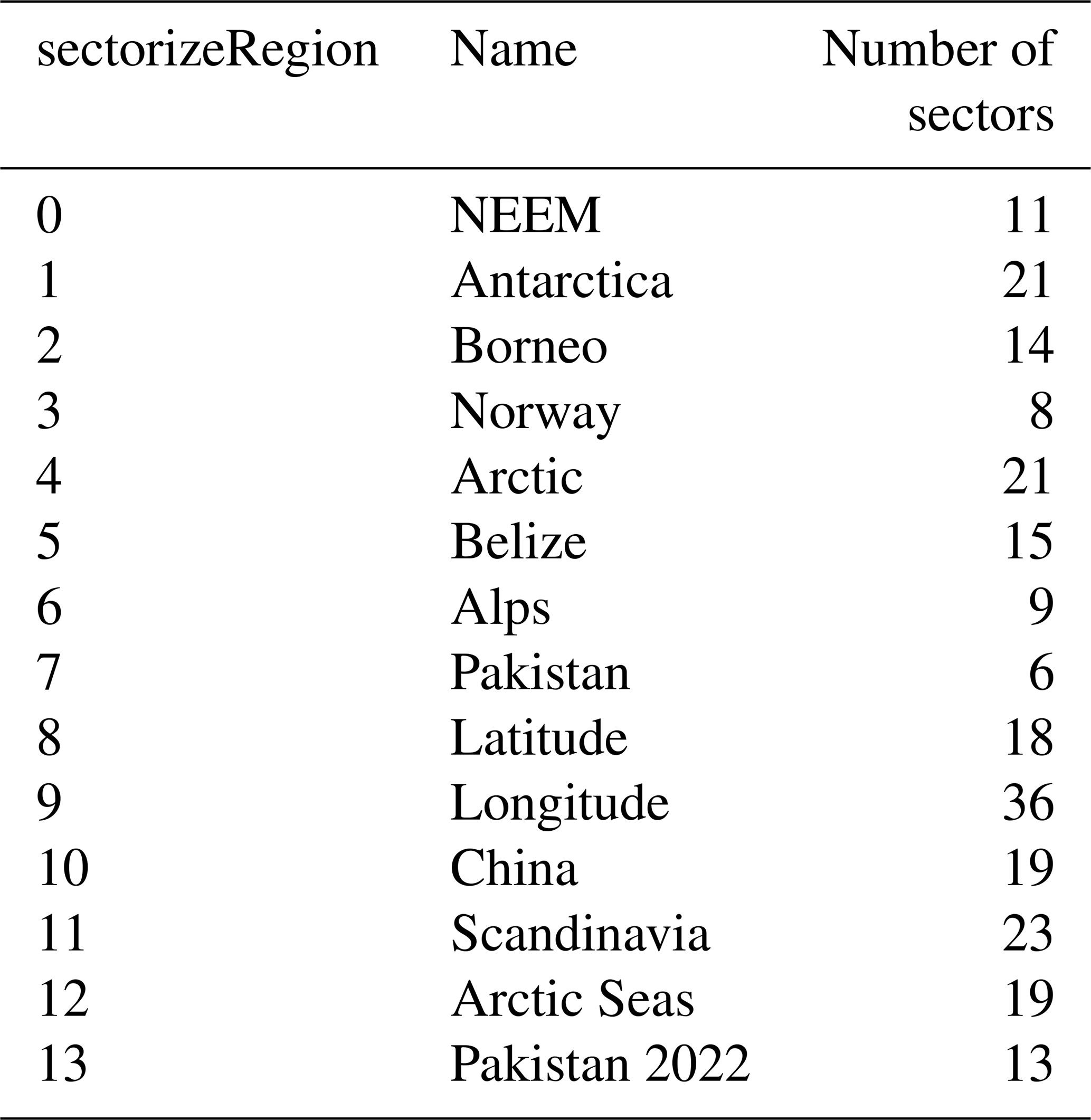
The sectorisation parameters allow to assign quantities on the moisture source and transport grid to pre-specified regions (Sect. 5.7). In total 14 sectorisations are currently built into the program code of WaterSip, covering different regions of the globe (Fig. C1, Table C1). The sectorisation is specified in the run setup using parameter sectorizeRegion in settings group Case. Each of the sectors distinguishes between the respective land and ocean area. During post-processing, it is common to combine several sectors together to obtain desired information over a source region with more complex shape than a box. Users can define new sectorisations by modifying the program code in class Sectors (files Sectors.cpp, Sectors.h).
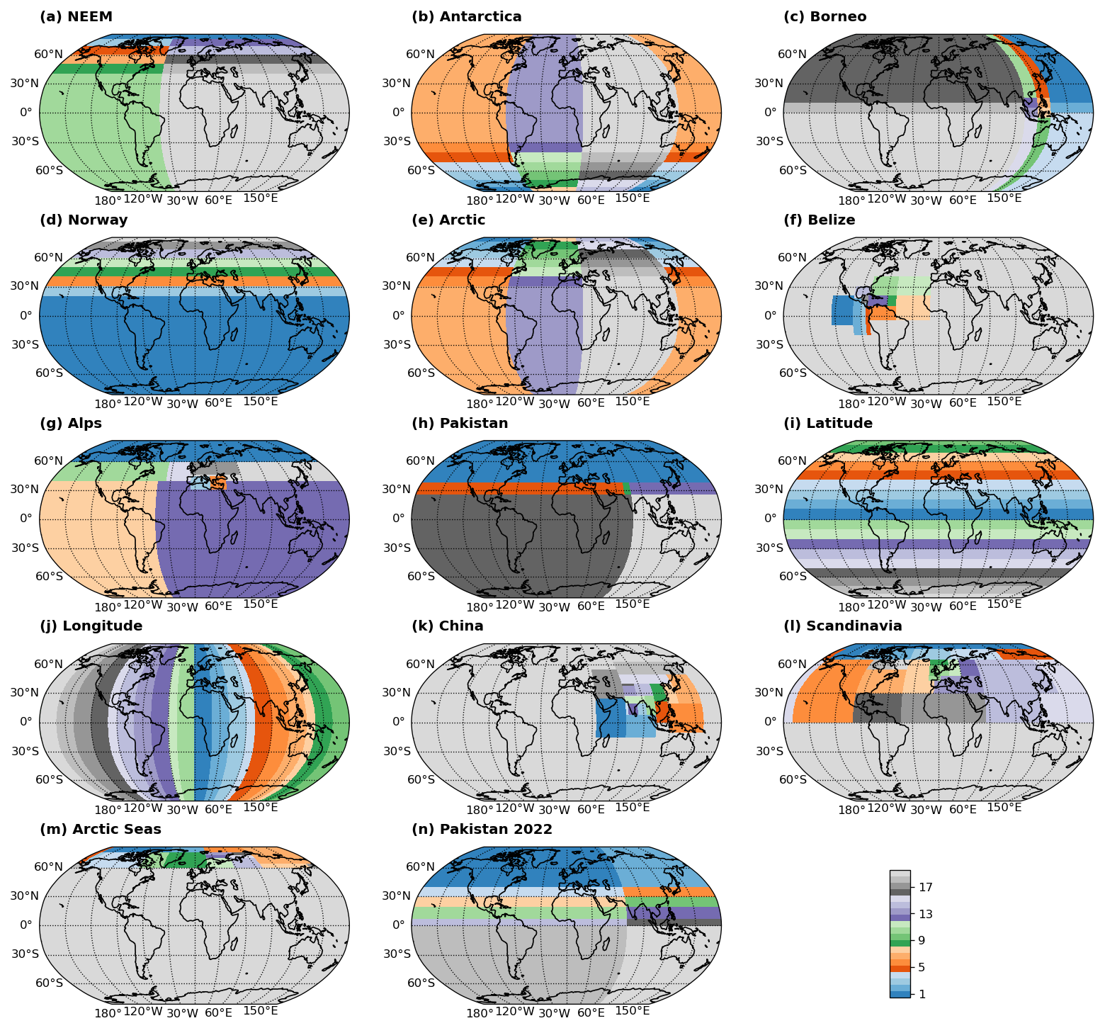
Figure C1Pre-defined sectorisations that are currently available in WaterSip. (a) NEEM sectorisation (11 sectors), (b) Antarctica sectorisation (21 sectors), (c) Borneo sectorisation (14 sectors), (d) Norway sectorisation (8 sectors), (e) Arctic sectorisation (21 sectors), (f) Belize sectorisation (15 sectors), (g) Alps sectorisation (9 sectors), (h) Pakistan sectorisation (6 sectors), (i) Latitude sectorisation (18 Sectors), (j) Longitude sectorisation (36 sectors), (k) China sectorisation (19 sectors), (l) Scandinavia sectorisation (23 sectors), (m) Arctic Seas sectorisation (19 sectors), (n) Pakistan 2022 sectorisation (13 sectors). Colour bar symbolic.
WaterSip creates a range of output files with different formats (Sect. 4.3 and Table 2). The primary results from the diagnostic are contained in the grid and series files. While grid files contain the spatially resolved information for different averaging intervals (time step, daily, monthly, yearly, and whole analysis period), the series files contain statistical properties (sum or mean, standard deviation, minimum and maximum) per averaging time. The source and transport properties are contained in grid and series files (Table D1), together with arrival and forward-projected quantities (Table D2).
The series file furthermore contains the results of the sectorisation (Sect. 5.7). Sectorisation variables comprise the sector area, as well as a percent fraction of the source and transport properties available on the global map per sector (Table D3). The sector information is separated into land and sea fractions, whereby the sector number can be accessed along the dimension sector.
Table D1Source and transport quantities contained in the grid and series files. Each variable is available as the sum, the standard deviation over the non-zero grid points, and the minimum and maximum value of the respective averaging interval. For step files, the precipitation rate is given per time step Δt, for all other files the rate is per day.
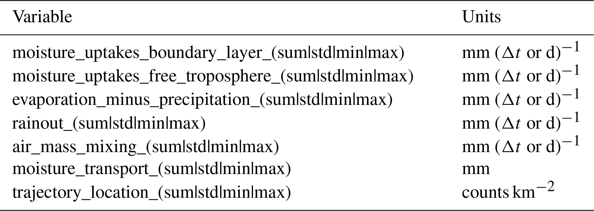
Table D2Arrival and Lagrangian forward projected properties contained in the grid files. * denotes variables weighted in addition by the Lagrangian precipitation estimate . + denotes variables weighted by the accounted fraction.
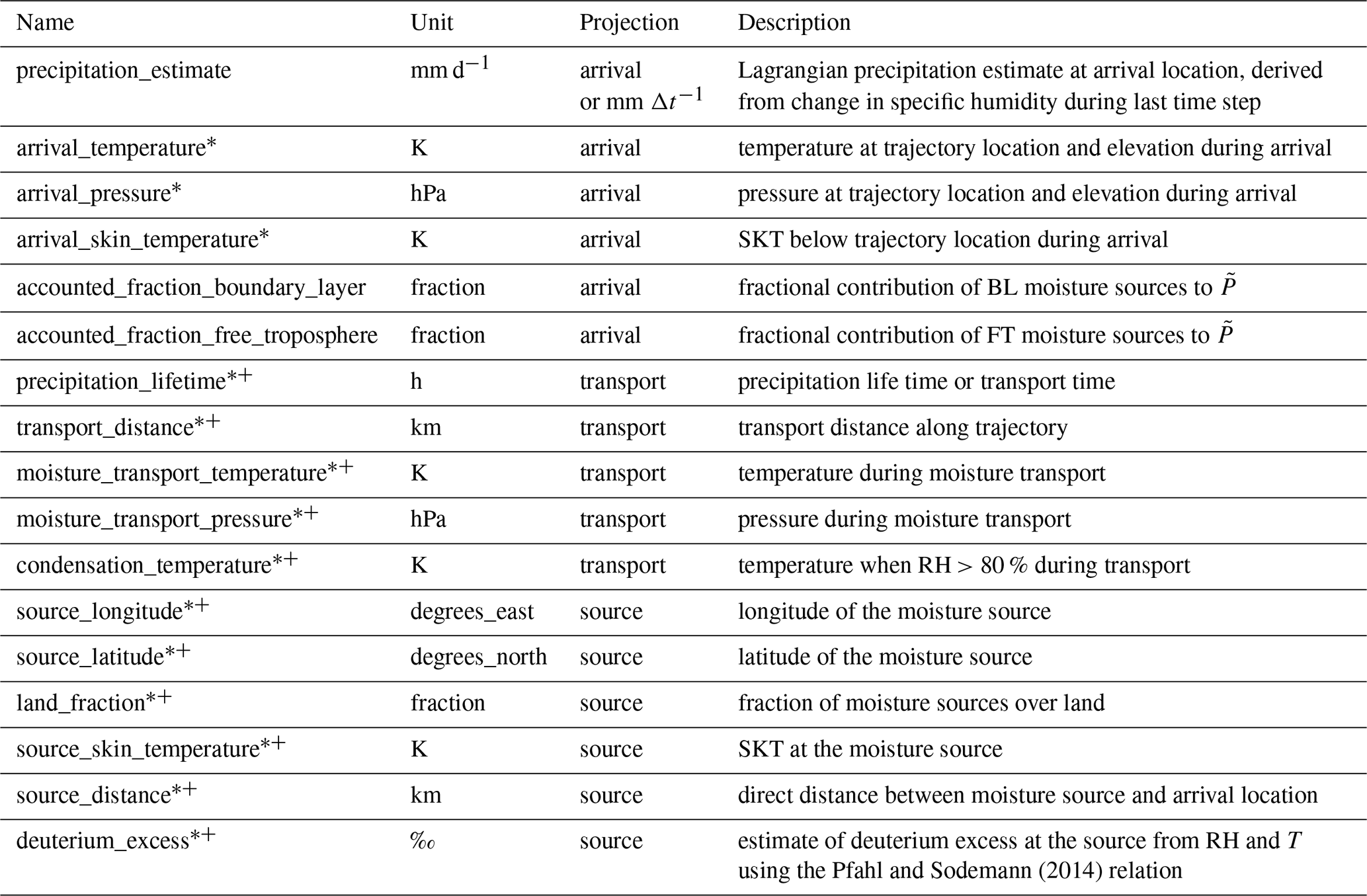
Table D3Sectorisation variables contained in the series files.
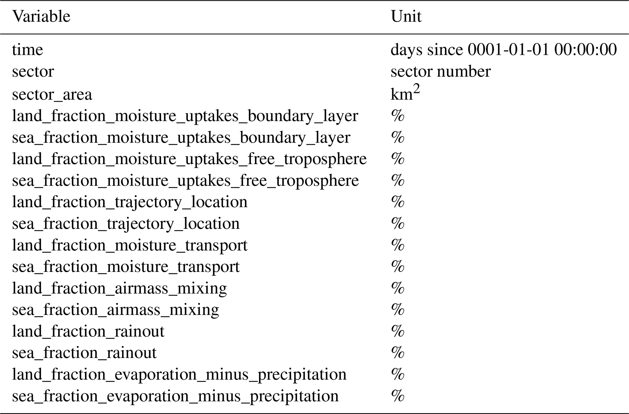
The model code of the WaterSip diagnostic in its current version 3.2.1 is available as archived code at https://doi.org/10.5281/zenodo.15068065 (Sodemann, 2025b) and maintained at the git repository https://git.app.uib.no/GFI-public/watersip (last access: 20 November 2025). Test data sets with FLEXPART output and corresponding WaterSip results are available at https://doi.org/10.5281/zenodo.14836548 (Sodemann, 2025a).
The author has declared that there are no competing interests.
Publisher’s note: Copernicus Publications remains neutral with regard to jurisdictional claims made in the text, published maps, institutional affiliations, or any other geographical representation in this paper. While Copernicus Publications makes every effort to include appropriate place names, the final responsibility lies with the authors. Views expressed in the text are those of the authors and do not necessarily reflect the views of the publisher.
I would like to acknowledge the many colleagues who contributed through their interest and comments, curiosity and critical questions to the further development of the WaterSip tool, in particular Alexander Läderach, Astrid Fremme, Yongbiao Weng, Mika Lanzky, and Matthew Osman. Marte Hofsteenge and Costijn Zwart are kindly acknowledged for providing helpful comments to an earlier version of this manuscript. I also want to thank Marina Dütsch and an anonymous reviewer for their detailed and constructive comments. The computations were performed on resources provided by Sigma2 - the National Infrastructure for High-Performance Computing and Data Storage in Norway.
This research has been supported by the Norges Forskningsråd (grant no. 262710) and the European Research Council (ERC) within the EU's H2020 research programme (grant no. 773245).
This paper was edited by Penelope Maher and reviewed by Marina Duetsch and one anonymous referee.
Aemisegger, F., Pfahl, S., Sodemann, H., Lehner, I., Seneviratne, S. I., and Wernli, H.: Deuterium excess as a proxy for continental moisture recycling and plant transpiration, Atmos. Chem. Phys., 14, 4029–4054, https://doi.org/10.5194/acp-14-4029-2014, 2014. a, b, c
Araguás-Araguás, L., Froehlich, K., and Rozanski, K.: Deuterium and oxygen-18 isotope composition of precipitation and atmospheric moisture, Hydrological Processes, 14, 1341–1355, https://doi.org/10.1002/1099-1085(20000615)14:8<1341::AID-HYP983>3.0.CO;2-Z, 2000. a
Bakels, L., Tatsii, D., Tipka, A., Thompson, R., Dütsch, M., Blaschek, M., Seibert, P., Baier, K., Bucci, S., Cassiani, M., Eckhardt, S., Groot Zwaaftink, C., Henne, S., Kaufmann, P., Lechner, V., Maurer, C., Mulder, M. D., Pisso, I., Plach, A., Subramanian, R., Vojta, M., and Stohl, A.: FLEXPART version 11: improved accuracy, efficiency, and flexibility, Geosci. Model Dev., 17, 7595–7627, https://doi.org/10.5194/gmd-17-7595-2024, 2024. a, b
Baker, A., Sodemann, H., Baldini, J. U. L., Breitenbach, S. F. M., Johnson, K. R., van Hunen, J., and Pingzhong, Z.: Seasonality of westerly moisture transport in the East Asian Summer Monsoon and its implications for interpreting precipitation δ18O, J. Geophys. Res., 120, https://doi.org/10.1002/2014JD022919, 2015. a, b
Bohlinger, P., Sorteberg, A., and Sodemann, H.: Synoptic conditions and moisture sources actuating extreme precipitation in Nepal, Journal of Geophysical Research: Atmospheres, 122, 12653–12671, https://doi.org/10.1002/2017JD027543, 2017. a
Bohlinger, P., Sorteberg, A., Liu, C., Rasmussen, R., Sodemann, H., and Ogawa, F.: Multiscale characteristics of an extreme precipitation event over Nepal, QJRMS, 18 pp., https://doi.org/10.1002/qj.3418, 2018. a
Bonne, J.-L., Masson-Delmotte, V., Cattani, O., Delmotte, M., Risi, C., Sodemann, H., and Steen-Larsen, H. C.: The isotopic composition of water vapour and precipitation in Ivittuut, southern Greenland, Atmos. Chem. Phys., 14, 4419–4439, https://doi.org/10.5194/acp-14-4419-2014, 2014. a
Bonne, J.-L., Steen-Larsen, H. C., Risi, C., Werner, M., Sodemann, H., Lacour, J.-L., Fettweis, X., Cesana, G., Delmotte, M., Cattani, O., Vallelonga, P., Kjær, H. A., Clerbaux, C., Sveinbjörnsdóttir, A. E., and Masson-Delmotte, V.: The summer 2012 Greenland heat wave: In situ and remote sensing observations of water vapor isotopic composition during an atmospheric river event, J. Geophys. Res., 120, 2970–2989, https://doi.org/10.1002/2014JD022602, 2015. a
Breitenbach, S. F., Adkins, J. F., Meyer, H., Marwan, N., Kumar, K. K., and Haug, G. H.: Strong influence of water vapor source dynamics on stable isotopes in precipitation observed in Southern Meghalaya, NE India, Earth and Planetary Science Letters, 292, 212–220, https://doi.org/10.1016/j.epsl.2010.01.038, 2010. a
Brubaker, K. L., Entekhabi, D., and Eagleson, P. S.: Estimation of continental precipitation recycling, J. Climate, 6, 1077–1089, https://doi.org/10.1175/1520-0442(1993)006<1077:EOCPR>2.0.CO;2, 1993. a
Brubaker, K. L., Dirmeyer, P. A., Sudradjat, A., Levy, B. S., and Bernal, F.: A 36-yr climatological description of the evaporative sources of warm-season precipitation in the Mississippi river basin, J. Hydrometeorol., 2, 537–557, https://doi.org/10.1175/1525-7541(2001)002<0537:AYCDOT>2.0.CO;2, 2001. a
Buizert, C., Sigl, M., Severi, M., Markle, B., Wettstein, J., McConnell, J., Pedro, J., Sodemann, H., Goto-Azuma, K., Kawamura, K., Fujita, S., Motoyama, H., Hirabayashi, M., Uemura, R., Stenni, B., Parrenin, F., He, F., Fudge, T., and Steig, E. J.: Abrupt ice-age shifts in southern westerly winds and Antarctic climate forced from the north, Nature, 563, 681–685, 2018. a
Dirmeyer, P. A. and Brubaker, K. L.: Contrasting evaporative moisture sources during the drought of 1988 and the flood of 1993, J. Geophys. Res., 104, 19383–19397, https://doi.org/10.1029/1999JD900222, 1999. a, b, c, d, e
Dominguez, F., Miguez-Macho, G., and Hu, H.: WRF with Water Vapor Tracers: A Study of Moisture Sources for the North American Monsoon, Journal of Hydrometeorology, 17, 1915–1927, https://doi.org/10.1175/JHM-D-15-0221.1, 2016. a
Dominguez, F., Hu, H., and Martinez, J. A.: Two-Layer Dynamic Recycling Model (2L-DRM): Learning from Moisture Tracking Models of Different Complexity, Journal of Hydrometeorology, 21, 3 – 16, https://doi.org/10.1175/JHM-D-19-0101.1, 2020. a
Dütsch, M., Pfahl, S., Meyer, M., and Wernli, H.: Lagrangian process attribution of isotopic variations in near-surface water vapour in a 30-year regional climate simulation over Europe, Atmos. Chem. Phys., 18, 1653–1669, https://doi.org/10.5194/acp-18-1653-2018, 2018. a, b, c, d, e
Eltahir, E. A. B. and Bras, R. L.: Precipitation recycling in the Amazon basin, Q. J. Roy. Meteor. Soc., 120, 861–880, https://doi.org/10.1002/qj.49712051806, 1994. a
Eltahir, E. A. B. and Bras, R. L.: Precipitation recycling, Reviews of Geophysics, 34, 367–378, https://doi.org/10.1029/96RG01927, 1996. a
Fernández-Alvarez, J. C., Pérez-Alarcón, A., Nieto, R., and Gimeno, L.: TROVA: TRansport Of water VApor, SoftwareX, 20, 101228, https://doi.org/10.1016/j.softx.2022.101228, 2022. a
Flatau, P. J., Walko, R. L., and Cotton, W. R.: Polynomial Fits to Saturation Vapor Pressure, Journal of Applied Meteorology and Climatology, 31, 1507–1513, https://doi.org/10.1175/1520-0450(1992)031<1507:PFTSVP>2.0.CO;2, 1992. a
Fremme, A. and Sodemann, H.: The role of land and ocean evaporation on the variability of precipitation in the Yangtze River valley, Hydrol. Earth Syst. Sci., 23, 2525–2540, https://doi.org/10.5194/hess-23-2525-2019, 2019. a, b, c, d
Fremme, A., Hezel, P. J., Seland, Ø., and Sodemann, H.: Model-simulated hydroclimate in the East Asian summer monsoon region during past and future climate: a pilot study with a moisture source perspective, Weather Clim. Dynam., 4, 449–470, https://doi.org/10.5194/wcd-4-449-2023, 2023. a, b, c, d, e, f, g, h, i
Gimeno, L., Eiras-Barca, J., Durán-Quesada, A. M., Dominguez, F., van der Ent, R., Sodemann, H., Sánchez-Murillo, R., Nieto, R., and Kirchner, J. W.: The residence time of water vapour in the atmosphere, Nature Reviews Earth & Environment, 2, 558–569, https://doi.org/10.1038/s43017-021-00181-9, 2021. a, b, c, d
Gustafsson, M., Rayner, D., and Chen, D.: Extreme rainfall events in southern Sweden: where does the moisture come from?, Tellus A, 62, 605–616, https://doi.org/10.1111/j.1600-0870.2010.00456.x, 2010. a, b, c, d, e
Hirdman, D., Sodemann, H., Eckhardt, S., Burkhart, J. F., Jefferson, A., Mefford, T., Quinn, P. K., Sharma, S., Ström, J., and Stohl, A.: Source identification of short-lived air pollutants in the Arctic using statistical analysis of measurement data and particle dispersion model output, Atmos. Chem. Phys., 10, 669–693, https://doi.org/10.5194/acp-10-669-2010, 2010. a
Hofsteenge, M. G., Cullen, N. J., Sodemann, H., and Katurji, M.: Synoptic Drivers and Moisture Sources of Snowfall in Coastal Victoria Land, Antarctica, Journal of Geophysical Research: Atmospheres, 130, e2024JD042021, https://doi.org/10.1029/2024JD042021, 2025. a
Holgate, C. M., Van Dijk, A. I. J. M., Evans, J. P., and Pitman, A. J.: Local and Remote Drivers of Southeast Australian Drought, Geophysical Research Letters, 47, e2020GL090238, https://doi.org/10.1029/2020GL090238, 2020. a
Johnsen, S. J., Dansgaard, W., and White, J. W. C.: The origin of Arctic precipitation under present and glacial conditions, Tellus B, 41B, 452–468, https://doi.org/10.1111/j.1600-0889.1989.tb00321.x, 1989. a
Keune, J., Schumacher, D. L., and Miralles, D. G.: A unified framework to estimate the origins of atmospheric moisture and heat using Lagrangian models, Geosci. Model Dev., 15, 1875–1898, https://doi.org/10.5194/gmd-15-1875-2022, 2022. a
Laederach, A.: Characteristic scales of atmospheric moisture transport, Ph.D. thesis, ETH Zurich, Diss ETH No. 23586, https://doi.org/10.3929/ethz-a-010741025, 2016. a
Laederach, A. and Sodemann, H.: A revised picture of the atmospheric residence time of water vapour, Geophys. Res. Lett., 43, 924–933, https://doi.org/10.1002/2015GL067449, 2016. a, b, c, d, e, f
Martius, O., Sodemann, H., Joos, H., Pfahl, S., Winschall, A., Croci-Maspoli, M., Graf, M., Madonna, E., Mueller, B., Schemm, S., Sedlacek, J., Sprenger, M., and Wernli, H.: The role of upper-level dynamics and surface processes for the Pakistan flood in July 2010, Q. J. Roy. Meteor. Soc., https://doi.org/10.1002/qj.2082, 2012. a, b
Masson-Delmotte, V., Buiron, D., Ekaykin, A., Frezzotti, M., Gallée, H., Jouzel, J., Krinner, G., Landais, A., Motoyama, H., Oerter, H., Pol, K., Pollard, D., Ritz, C., Schlosser, E., Sime, L. C., Sodemann, H., Stenni, B., Uemura, R., and Vimeux, F.: A comparison of the present and last interglacial periods in six Antarctic ice cores, Clim. Past, 7, 397–423, https://doi.org/10.5194/cp-7-397-2011, 2011. a
Miltenberger, A. K., Pfahl, S., and Wernli, H.: An online trajectory module (version 1.0) for the nonhydrostatic numerical weather prediction model COSMO, Geosci. Model Dev., 6, 1989–2004, https://doi.org/10.5194/gmd-6-1989-2013, 2013. a
Moerman, J. W., Cobb, K. M., Adkins, J. F., Sodemann, H., Clark, B., and Tuen, A. A.: Diurnal to interannual rainfall δ18O variations in northern Borneo driven by regional hydrology, Earth and Planetary Science Letters, 369–370, 108–119, https://doi.org/10.1016/j.epsl.2013.03.014, 2013. a
Numaguti, A.: Origin and recycling processes of precipitating water over the Eurasian continent: Experiments using an atmospheric general circulation model, J. Geophys. Res., 104, 1957–1972, https://doi.org/10.1029/1998JD200026, 1999. a
Osman, M. B., Smith, B. E., Trusel, L. D., Das, S. B., McConnell, J. R., Chellman, N., Arienzo, M., and Sodemann, H.: Abrupt Common Era hydroclimate shifts drive west Greenland ice cap change, Nature Geoscience, 14, 756–761, https://doi.org/10.1038/s41561-021-00818-w, 2021. a
Pfahl, S. and Sodemann, H.: What controls deuterium excess in global precipitation?, Clim. Past, 10, 771–781, https://doi.org/10.5194/cp-10-771-2014, 2014. a, b, c, d
Pisso, I., Sollum, E., Grythe, H., Kristiansen, N. I., Cassiani, M., Eckhardt, S., Arnold, D., Morton, D., Thompson, R. L., Groot Zwaaftink, C. D., Evangeliou, N., Sodemann, H., Haimberger, L., Henne, S., Brunner, D., Burkhart, J. F., Fouilloux, A., Brioude, J., Philipp, A., Seibert, P., and Stohl, A.: The Lagrangian particle dispersion model FLEXPART version 10.4, Geosci. Model Dev., 12, 4955–4997, https://doi.org/10.5194/gmd-12-4955-2019, 2019. a, b
Salati, E., Dall'Olio, A., Matsui, E., and Gat, J. R.: Recycling of water in the Amazon Basin: An isotopic study, Water Resources Research, 15, 1250–1258, https://doi.org/10.1029/WR015i005p01250, 1979. a
Singh, H. K. A., Bitz, C. M., Donohoe, A., and Rasch, P. J.: A Source–Receptor Perspective on the Polar Hydrologic Cycle: Sources, Seasonality, and Arctic–Antarctic Parity in the Hydrologic Cycle Response to CO2 Doubling, Journal of Climate, 30, 9999–10017, https://doi.org/10.1175/JCLI-D-16-0917.1, 2017. a
Sodemann, H.: Beyond turnover time: Constraining the lifetime distribution of water vapor from simple and complex approaches, Journal of the Atmospheric Sciences, 77, 413–433, https://doi.org/10.1175/JAS-D-18-0336.1, 2020. a, b, c, d, e, f, g, h
Sodemann, H.: Source code of the Lagrangian moisture source and transport diagnostic WaterSip V3.2.1, Zenodo [code], https://doi.org/10.5281/zenodo.15068065, 2025a. a, b, c, d, e
Sodemann, H.: Particle position output from the FLEXPART dispersion model for a test case for use with the WaterSip moisture source diagnostic, Zenodo [data set], https://doi.org/10.5281/zenodo.14836548, 2025b. a, b
Sodemann, H. and Stohl, A.: Asymmetries in the moisture origin of Antarctic precipitation, Geophys. Res. Lett., 36, L22803, https://doi.org/10.1029/2009GL040242, 2009. a, b, c, d, e, f
Sodemann, H. and Zubler, E.: Seasonal and inter-annual variability of the moisture sources for Alpine precipitation during 1995-2002, Int. J. Climatol., 30, 947–961, https://doi.org/10.1002/joc.1932, 2010. a, b, c, d, e, f
Sodemann, H., Masson-Delmotte, V., Schwierz, C., Vinther, B. M., and Wernli, H.: Interannual variability of Greenland winter precipitation sources: 2. Effects of North Atlantic Oscillation variability on stable isotopes in precipitation, J. Geophys. Res., 113, D12111, https://doi.org/10.1029/2007JD009416, 2008a. a, b, c
Sodemann, H., Schwierz, C., and Wernli, H.: Interannual variability of Greenland winter precipitation sources: Lagrangian moisture diagnostic and North Atlantic Oscillation influence, J. Geophys. Res., 113, D03107, https://doi.org/10.1029/2007JD008503, 2008b. a, b, c, d, e, f, g, h, i, j, k, l, m, n, o, p, q, r, s, t, u, v, w, x, y
Sprenger, M. and Wernli, H.: The LAGRANTO Lagrangian analysis tool – version 2.0, Geosci. Model Dev., 8, 2569–2586, https://doi.org/10.5194/gmd-8-2569-2015, 2015. a, b, c
Steen-Larsen, H. C., Sveinbjörnsdottir, A. E., Jonsson, T., Ritter, F., Bonne, J.-L., Masson-Delmotte, V., Sodemann, H., Blunier, T., Dahl-Jensen, D., and Vinther, B. M.: Moisture sources and synoptic to seasonal variability of North Atlantic water vapor isotopic composition, J. Geophys. Res., 120, 5757–5774, https://doi.org/10.1002/2015JD023234, 2015. a
Stohl, A.: Computation, accuracy and applications of trajectories–A review and bibliography, Atmos. Environ., 32, 947–966, ISSN 1352-2310, https://doi.org/10.1016/S1352-2310(97)00457-3, 1998. a, b
Stohl, A.: Characteristics of atmospheric transport into the Arctic troposphere, Journal of Geophysical Research: Atmospheres, 111, https://doi.org/10.1029/2005JD006888, 2006. a
Stohl, A. and James, P.: A Lagrangian analysis of the atmospheric branch of the global water cycle. Part I: Method description, validation, and demonstration for the August 2002 flooding in Central Europe, J. Hydrometeorol., 5, 656–678, https://doi.org/10.1175/1525-7541(2004)005<0656:ALAOTA>2.0.CO;2, 2004. a, b, c, d, e, f, g, h, i, j
Stohl, A. and James, P.: A Lagrangian analysis of the atmospheric branch of the global water cycle. Part II: Moisture transports between earth’s ocean basins and river catchments, J. Hydrometeorol., 6, 961–984, https://doi.org/10.1175/JHM470.1, 2005. a, b
Stohl, A., Forster, C., Frank, A., Seibert, P., and Wotawa, G.: Technical note: The Lagrangian particle dispersion model FLEXPART version 6.2, Atmos. Chem. Phys., 5, 2461–2474, https://doi.org/10.5194/acp-5-2461-2005, 2005. a, b, c
Terpstra, A., Gorodetskaya, I. V., and Sodemann, H.: Linking Sub-Tropical Evaporation and Extreme Precipitation Over East Antarctica: An Atmospheric River Case Study, Journal of Geophysical Research: Atmospheres, 126, e2020JD033617, https://doi.org/10.1029/2020JD033617, 2021. a, b
Trenberth, K. E., Smith, L., Qian, T., Dai, A., and Fasullo, J.: Estimates of the Global Water Budget and Its Annual Cycle Using Observational and Model Data, Journal of Hydrometeorology, 8, 758–769, https://doi.org/10.1175/JHM600.1, 2007. a
van der Ent, R. J., Tuinenburg, O. A., Knoche, H.-R., Kunstmann, H., and Savenije, H. H. G.: Should we use a simple or complex model for moisture recycling and atmospheric moisture tracking?, Hydrol. Earth Syst. Sci., 17, 4869–4884, https://doi.org/10.5194/hess-17-4869-2013, 2013. a
van der Ent, R. J., Wang-Erlandsson, L., Keys, P. W., and Savenije, H. H. G.: Contrasting roles of interception and transpiration in the hydrological cycle – Part 2: Moisture recycling, Earth Syst. Dynam., 5, 471–489, https://doi.org/10.5194/esd-5-471-2014, 2014. a, b
Škerlak, B., Sprenger, M., and Wernli, H.: A global climatology of stratosphere–troposphere exchange using the ERA-Interim data set from 1979 to 2011, Atmos. Chem. Phys., 14, 913–937, https://doi.org/10.5194/acp-14-913-2014, 2014. a
Wang, Y., Sodemann, H., Hou, S., Masson-Delmotte, V., Jouzel, J., and Pang, H.: Snow accumulation and its moisture origin over Dome Argus, Antarctica, Climate Dynamics, 40, 731–742, https://doi.org/10.1007/s00382-012-1398-9, 2013. a
Weng, Y., Johannessen, A., and Sodemann, H.: High-resolution stable isotope signature of a land-falling atmospheric river in southern Norway, Weather Clim. Dynam., 2, 713–737, https://doi.org/10.5194/wcd-2-713-2021, 2021. a, b, c, d, e
Winkler, R., Landais, A., Sodemann, H., Dümbgen, L., Prié, F., Masson-Delmotte, V., Stenni, B., and Jouzel, J.: Deglaciation records of 17O-excess in East Antarctica: reliable reconstruction of oceanic normalized relative humidity from coastal sites, Clim. Past, 8, 1–16, https://doi.org/10.5194/cp-8-1-2012, 2012. a
Winschall, A., Pfahl, S., Sodemann, H., and Wernli, H.: Comparison of Eulerian and Lagrangian moisture source diagnostics – the flood event in eastern Europe in May 2010, Atmos. Chem. Phys., 14, 6605–6619, https://doi.org/10.5194/acp-14-6605-2014, 2014a. a, b, c
Winschall, A., Sodemann, H., Pfahl, S., and Wernli, H.: How important is intensified evaporation for Mediterranean precipitation extremes?, J. Geophys. Res., 119, 5240–5256, https://doi.org/10.1002/2013JD021175, 2014b. a, b, c, d
Yoshimura, K., Oki, T., Ohte, N., and Kanae, S.: Colored Moisture Analysis Estimates of Variations in 1998 Asian Monsoon Water Sources, Journal of the Meteorological Society of Japan, 82, 1315–1329, https://doi.org/10.2151/jmsj.2004.1315, 2004. a
Zannoni, D., Steen-Larsen, H. C., Peters, A. J., Wahl, S., Sodemann, H., and Sveinbjörnsdóttir, A. E.: Non-Equilibrium Fractionation Factors for D/H and 18O/16O During Oceanic Evaporation in the North-West Atlantic Region, Journal of Geophysical Research: Atmospheres, 127, e2022JD037076, https://doi.org/10.1029/2022JD037076, 2022. a
The name WaterSip originates from the name of an internal research project at NILU, where the author developed large parts of the present code. The name can be understood as a metaphor, where increases of the water vapour mixing ratio between time steps could be imagined as sips of water taken by an air parcel.
- Abstract
- Introduction
- Method
- Configuration of WaterSip
- Setup and execution of WaterSip
- Diagnosed moisture source, transport and arrival properties
- Discussion
- Summary and Final Remarks
- Appendix A: Spatial characteristics of Lagrangian precipitation estimate
- Appendix B: Description of control parameters in the WaterSip configuration file
- Appendix C: Sectorisation options
- Appendix D: Output files
- Code and data availability
- Competing interests
- Disclaimer
- Acknowledgements
- Financial support
- Review statement
- References