Applications of Machine Learning and Artificial Intelligence in Tropospheric Ozone Research

Machine learning (ML) is transforming atmospheric chemistry, offering powerful tools to address challenges in tropospheric ozone research, a critical area for climate resilience and public health. As in adjacent fields, ML approaches complement existing research by learning patterns from ever-increasing volumes of atmospheric and environmental data relevant to ozone. We highlight the rapid progress made in the field since Phase 1 of the Tropospheric Ozone Assessment Report (TOAR), focussing particularly on the most active areas of research, namely short-term ozone forecasting, emulation of atmospheric chemistry and the use of remote sensing for ozone estimation. This review provides a comprehensive synthesis of recent advancements, highlights critical challenges, and proposes actionable pathways to develop ML in ozone research. Further advances hinge on addressing domain-specific issues such as the dependence of ozone concentrations on several poorly observed precursor species, as well as making progress on generic ML challenges such as the definition of suitable benchmarks and developing robust, explainable models. Reaping the full potential of ML for ozone research and operational applications will require close collaborations across atmospheric chemistry, ML and computational science and vigilant pursuit of the rapid developments in adjacent fields.

1 Introduction

The ML4O3 working group was established as part of the second phase of the IGAC Tropospheric Ozone Assessment Report (TOAR). The group focuses on the application of machine learning (ML) concepts and methods, promoting dialogue between researchers in machine learning and tropospheric ozone communities. The motivation of this group is to allow the atmospheric chemistry community to capitalize on the potential of ML and AI techniques that has recently been demonstrated for weather and climate applications. The ML tasks that were addressed by the group included identifying complex patterns, interpolating missing values, detecting errors or anomalies, and identifying air pollution regimes. The working group aimed to contribute to both fundamental scientific understanding of the processes controlling ozone, and to improved air quality monitoring and forecasting.

Tropospheric ozone is a harmful atmospheric pollutant and an important greenhouse gas, contributing to both environmental and public health issues. Long-term exposure to elevated ozone levels is linked to hundreds of thousands of premature deaths globally each year (Malashock et al., 2022; Malley et al., 2017; Health Effects Institute, 2024). Short-term exposure can cause serious negative health impacts (Bell et al., 2014) including reduced lung function, particularly in individuals with pre-existing medical conditions (EPA, 2020). Beyond its health impacts, tropospheric ozone significantly damages vegetation in natural ecosystems and agricultural fields (Mills et al., 2018) and can act as a climate forcer in the upper troposphere. In addition, ozone plays a critical role in tropospheric chemistry, both as a source of oxidants and as a primary oxidant itself (Monks et al., 2015).

Ozone is challenging to simulate accurately (Young et al., 2018), also for ML models, because it is not directly emitted into the troposphere but is photochemically produced in the presence of sunlight by reactions involving its precursor gases: carbon monoxide (CO), methane (CH₄), volatile organic compounds (VOCs), and nitrogen oxides (NO_x, NO+NO₂). In addition, ozone is transported from the stratosphere into the troposphere. The removal of tropospheric ozone is controlled by chemical loss and deposition to the surface (Archibald et al., 2020). The lifetime of ozone in the troposphere ranges from days to weeks, depending on local chemical and meteorological conditions (Lelieveld and Dentener, 2000; Monks et al., 2015). This variability allows ozone and its precursors to be transported over long distances from their sources (Fiore et al., 2009).

The complex coupling of these chemical and physical processes controls the local concentrations of ozone across different spatial and temporal scales, as detailed in Fig. 1. Traditionally, concentrations of ozone and other chemical species are calculated using numerical models of the atmosphere that represent these processes across a wide range of spatial scales, from high-resolution urban models (meter-scale) to global chemistry-climate models with resolutions ranging from tens to hundreds of kilometers (e.g. Morgenstern et al., 2017).

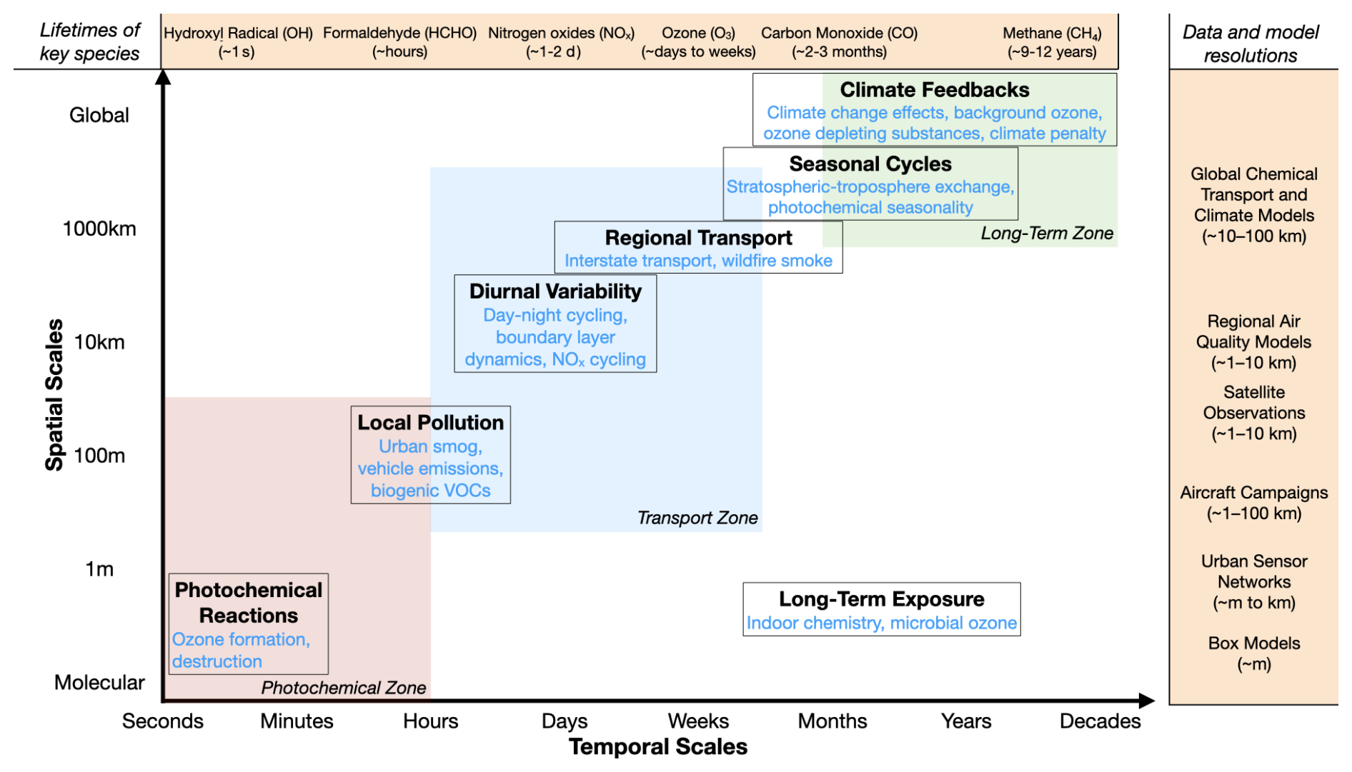
Figure 1 Spatial and temporal scales of tropospheric ozone chemistry processes. The x-axis shows timescales, from rapid photochemical reactions to long-term climate feedbacks, and the y-axis shows spatial scales, from local pollution to global atmospheric transport. Species lifetimes and relevant data sources and models are displayed to illustrate the range and scales of phenomena and methods used to study ozone chemistry.

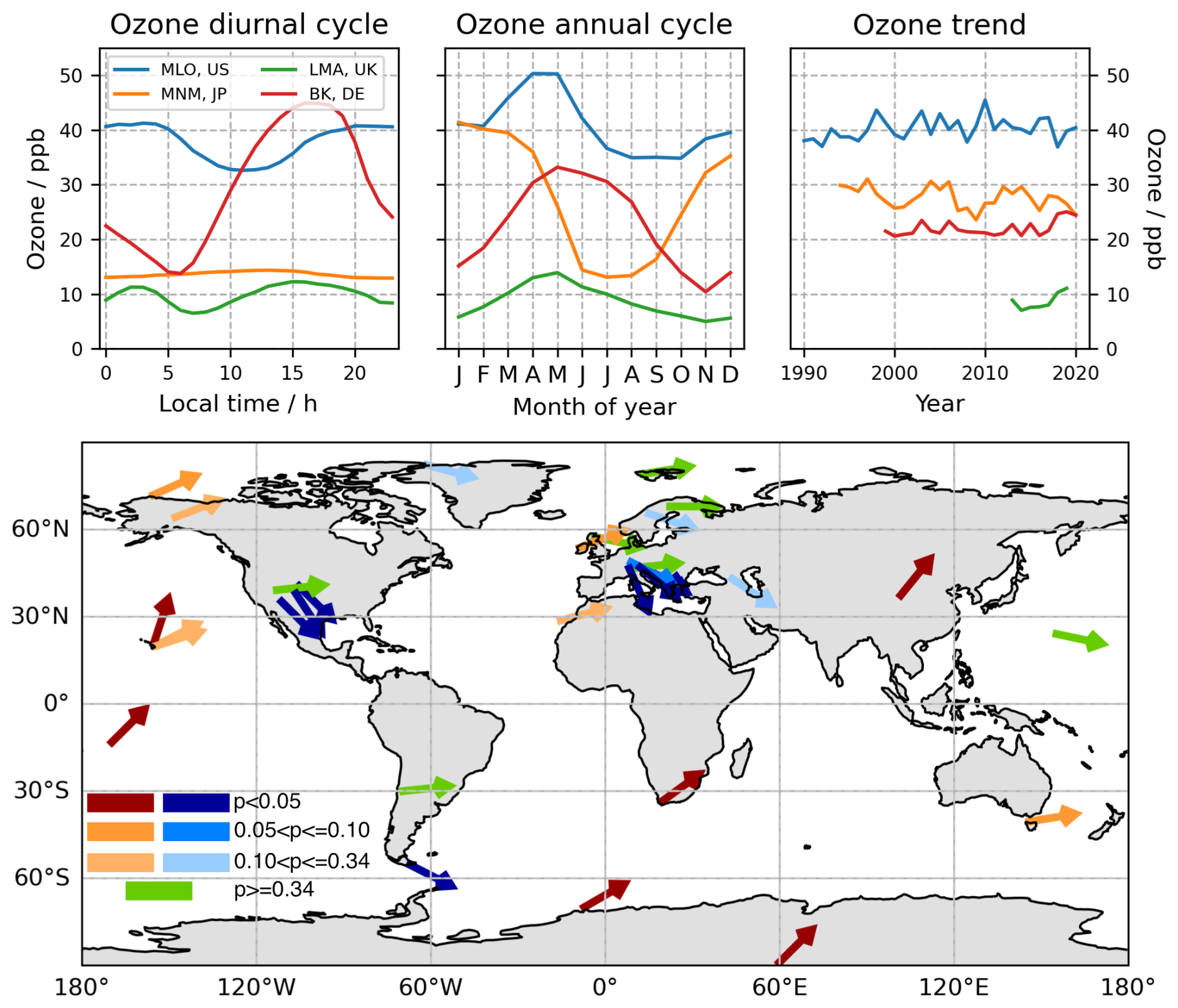
Figure 2 Upper panel: data from the TOAR ozone database for four sites in the northern hemisphere, showing diurnal and seasonal cycles in ozone, and the long-term ozone trend. MLO, US: Mauna Loa Observatory, US; MNM, JP: Minamitorishima, Japan; LMA, UK: Marylebone Road, London, UK; BK, DE: Borken, Germany. Lower panel: long-term ozone trends based on monthly anomalies at remote surface sites. Red and blue indicate positive or negative trends respectively, with different shades giving the statistical significance of the trend at each site. Data from Cooper et al. (2020) and replotted here.

Despite the success of ozone simulations in air quality and climate research, large uncertainties still exist in global model estimates of tropospheric ozone and its trends, although ozone is the longest- and most-measured trace gas in the observational record. Observations from ground stations, ozonesondes, and satellites indicate that tropospheric ozone has generally increased in recent decades (Ziemke et al., 2019; Young et al., 2018; Gulev et al., 2021). While global atmospheric chemistry models agree that the global tropospheric ozone burden has increased from pre-industrial times to the present day, they vary regarding the spatial distribution and magnitude of the increase (Skeie et al., 2020; Christiansen et al., 2022; Fiore et al., 2022). Potential sources driving this model bias include uncertainties in tropical emissions (Zhang et al., 2021), nonlinear NO_x-VOC chemistry (Shah et al., 2023), stratosphere-troposphere exchange (Neu et al., 2014), boundary layer mixing (Lu et al., 2019), missing chemical mechanisms such as halogen chemistry (Wang et al., 2015), and deposition (Clifton et al., 2020).

The variation of ozone at various scales is shown in Fig. 2. The figure shows the diurnal and annual cycles of ozone at four sites from the TOAR database: Mauna Loa Observatory, a Pacific mountain station, based in Hawaii, USA; Minamitorishima, a Pacific island station in Japan; a regional continental background site, Borken, Germany, and an urban, roadside site, Marylebone Road, London, UK. There is little consistency between the diurnal cycles at the various sites: the remote Pacific site sees little diurnal variation in ozone, but a strong seasonal cycle, with levels reaching a minimum in the summer. In contrast, the continental, rural background site in Germany has a strong diurnal cycle, peaking in the late afternoon, and a strong seasonal cycle with a summertime maximum. The observed long-term trends in ozone, although weak, also vary between the sites, with both modest increases (London Marylebone Road) and decreases (Minamitorishima). The lower panel shows variation in ozone trends across the globe, ranging between −3 and 3 ppbv yr⁻¹, across remote sites. These differences across ozone monitoring sites result from the complex interactions between precursor emissions, transport and chemical processes, meteorological drivers, and surface characteristics. Capturing the diversity of daily and seasonal cycles as well as trends is a key requisite of any ozone model.

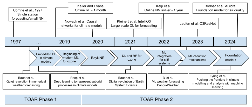
Figure 3 Timeline of a selection of studies using ML in ozone research (top), aligned with a selection of papers using ML in wider weather and climate modeling research (bottom). In both wider Earth system modeling research, and in ozone research there has been rapid progress over the last five years, as noted by landmark review papers highlighted in the Figure. The acronyms used are as follows. NN: neural network; RF: random forest; DL: deep learning; ML: machine learning.

Machine learning (ML) approaches, which can learn and reproduce nonlinear characteristics of a system from data (Hornik et al., 1989), may provide a valuable complement to physical models. As the quantity and quality of observational data on ozone (Schultz et al., 2017) and on the broader Earth system (Agapiou, 2017; Reichstein et al., 2019) continue to grow, ML is becoming an increasingly viable tool for advancing ozone research.

Figure 3 highlights progress in the field of ML as applied to weather and climate science, which has been rapid since the publication of the first phase of the TOAR assessment. In their review of the state of the field of weather forecasting, Bauer et al. (2015) note many areas of progress for the field, including model throughput, the process-level detail of then current models, and the use of data assimilation techniques to improve the fidelity of the model's initial state. The impact of ML methods was not anticipated. Rasp et al. (2018) demonstrated the potential for deep learning techniques to augment existing models in providing an alternative, complementary and physically consistent description of sub-grid scale processes, such as cloud microphysics. The coupling of a fast, accurate, data-driven module, trained on finer scale simulations, to a larger scale host climate model exemplified one of the potential ways that ML approaches can contribute to the improvement of climate and weather models. Subsequent studies have shown in various ways the advantages of ML over traditional numerical models, particularly in terms of computational efficiency and in the ability to learn from large datasets, as demonstrated by the success of data-driven nowcasting and weather forecasting models (Bi et al., 2023; Lam et al., 2023; Price et al., 2024).

Observational data, when integrated with model simulations through data assimilation techniques, have improved the understanding of emissions and atmospheric chemistry by reducing uncertainties (Miyazaki et al., 2020). ML can complement these efforts by combining observational data with model outputs, emulating model components, or enabling computationally cheaper simulations, thereby efficiently diagnosing sources of error in global atmospheric models and improving tropospheric ozone estimates. However, ML also has limitations, such as challenges in generalization, validation, and interpretability. Addressing these issues may be particularly relevant for the ozone modeling community where both predictive accuracy and physical understanding are valued.

In this Perspective, we provide an overview of the state of ML in tropospheric ozone research, review previous applications of ML to various problems related to ozone, and discuss persistent challenges and emerging opportunities. We highlight three areas where ML for ozone has been most widely applied: forecasts based on ground-based observations are reviewed in Sect. 2, methods for complementing or replacing parameterizations in numerical models of atmospheric chemistry and transport are discussed in Sect. 3, and ML models that use satellite data or combined data products are presented in Sect. 4. Section 5 highlights and further details these cross-cutting issues and limitations with the application of ML to ozone studies, while Sect. 6 describes future directions for the field, highlighting emerging approaches that seek to address the cross-cutting challenges.

2 Applications of ML to in-situ ozone observations: short-term ground level ozone forecasting

2.1 Background

The short-term forecasting of air pollutants including ozone, i.e. predictions of expected concentrations over 1–4 d, is relevant for public health and scientific questions (Buonocore et al., 2021; Hahm and Yoon, 2021; Alari et al., 2021; Saberian et al., 2017). State-of-the-art air quality forecasts, typically on the timescales of hours to days and up to a few days ahead, are based on the output of numerical chemical transport models (CTMs) (Marécal et al., 2015). These models may be run at higher spatial resolution for the area of interest (Savage et al., 2013), in order to better represent processes controlling air pollution at the local level, and may be post-processed to more accurately represent observations (Casciaro et al., 2022). As with other air pollutants, notably PM_2.5 (Feng et al., 2015), ML is increasingly being directly applied to the task of short-term, ground-level ozone forecasting, and to bias-correct existing air quality forecasting systems with considerable success. The availability of large and growing observational datasets has facilitated these advances (Schultz et al., 2017). However, forecasting ozone concentrations as time series with ML comes with significant challenges: forecasting ozone is a spatiotemporal problem, and ozone is controlled by processes of varying spatial and temporal scales as shown in Fig. 1.

Many short-term forecasting studies using ML have focused on forecasting only at selected observational stations, using observed ozone and additional chemical species, and meteorological variables where they are available from individual stations or external datasets (Comrie, 1997; Cobourn et al., 2000; Kolehmainen et al., 2001; Eslami et al., 2020; Sayeed et al., 2021; Leufen et al., 2023; Hickman et al., 2023). Furthermore, since it is difficult to downscale a relatively coarse CTM at specific locations, using time series data from a particular station is an attractive way to make predictions at particular locations. However, approaches of this kind do not necessarily provide ozone forecasts across all locations that may be of interest, as a gridded model product model might.

2.2 Progress and State of the Science

As with other fields, the advances in ML-based ozone forecasting have been pushed by developments on two axes – first, increasing quantities of data and second, larger models with more appropriate inductive biases. The field has a long history (see Fig. 3), with studies being published even during the most recent artificial intelligence (AI) “winter”, beginning with a feed-forward neural network (NN) in 1996 (Yi and Prybutok, 1996). Comrie (1997) illustrated that a NN could be used to forecast ozone at eight stations in the USA. This was followed by further feed-forward NN approaches, often with datasets drawn from a single location or city (Cobourn et al., 2000; Kolehmainen et al., 2001). Neural methods were typically evaluated in comparison with (autoregressive) regression models, often finding that NNs were better able to forecast ozone concentrations and extrema on test data (Nunnari et al., 1998; Schlink et al., 2003; Chaloulakou et al., 2003), although the improvement was often only marginal. Alongside the successes of feed-forward NN architectures, other work drew attention to methods seen to be more interpretable, such as fuzzy logic systems and regression trees (Gardner and Dorling, 2000; Heo and Kim, 2004). Further work leveraged methodological advances in ML architectures designed for temporal data, including the use of recurrent neural networks (RNNs) and convolutional neural networks (CNNs) to account for lagged relationships in the time series data (Eslami et al., 2020; Sayeed et al., 2021; Kleinert et al., 2021). Recent work has combined architectures to model the relationships that control ozone, including combining components such as transformers and CNNs to account for the temporal and spatial information relevant to forecasting (Chen et al., 2022; Cheng et al., 2022; Han et al., 2023). However, datasets have typically been limited to single countries or cities, due to the lack of a combined database of station measurements. The introduction of the TOAR surface database (Schultz et al., 2017) and the TOAR-II database have facilitated recent studies on data drawn from multiple countries (Leufen et al., 2023; Hickman et al., 2023). The importance of the curation of large datasets for scientific progress in ML is highlighted in the Outlook section.

Increasingly, more complex architectures are being used to enhance the accuracy of ozone forecasts, and more data are being included as input to the models. The inputs that are relevant to the physical drivers of ozone concentrations, such as past observations of ozone and covariates, and nearby covariates, reflect processes that control ozone observations, and feasibly contribute to improved ozone forecasting and infilling. Recently, methods on the scale of the ML architectures and data used for weather forecasting (Bi et al., 2023; Lam et al., 2023) have been transferred to ozone forecasting by leveraging very large datasets and models (Bodnar et al., 2024). In weather studies there is work on forecasting at observation stations using these methods, and transferring these methods to forecast ozone at ground-level stations is feasible (Manshausen et al., 2024).

3 Applications of ML methods in atmospheric chemistry modeling

3.1 Background

Global modeling of atmospheric chemistry is a grand computational challenge due to the high dimensionality of coupled chemical species, the nonlinearity and numerical stiffness of solving chemical mechanisms, and interactions with transport on all scales. The inclusion of comprehensive atmospheric chemistry in Earth system models (ESMs), which simulate the interactions between the atmosphere, oceans, land surface, and biosphere, is a priority science frontier (National Research Council (U.S.), 2012). Atmospheric chemical mechanisms are typically implemented in CTMs, which focus on the distribution and chemical evolution of species in the atmosphere. For some applications, chemistry-climate models (CCMs) may also couple chemical processes with climate dynamics, allowing feedback between chemistry and climate. Current atmospheric chemistry models integrate the coupled chemical kinetic equations for mechanism species over model time steps using high-order implicit numerical solvers, but these solvers are computationally expensive (Sandu et al., 1997) and often dominate the cost of an atmospheric simulation (Eastham et al., 2018). Such costs put the inclusion of atmospheric chemistry in tension with other computationally intensive ESM/CCM priorities such as increased spatial resolution and ensemble simulations. The current slowdown in the rate of increase in the speed of computer CPUs – the “end of Moore's law” – underscores the need for computationally efficient approaches (Theis and Wong, 2017).

Chemical solvers in atmospheric models compute the local evolution of species concentrations over a chemical time step that may range from minutes to hours depending on the model (Brasseur and Jacob, 2017). The chemical mechanisms used in regional to global atmospheric models and ESMs typically include 𝒪(100) coupled species with chemical lifetimes ranging from less than a second to much larger than the model time step. High-order implicit solvers can integrate this system of stiff coupled differential equations with high accuracy and fast implementations of these schemes are available, but they are still extremely costly for atmospheric models. Atmospheric models may combat that cost by decreasing the size of the chemical mechanism, breaking down the stiffness of the problem, or using lower-order approximations. However, these methods rarely achieve a speedup of more than a factor of two (Lin et al., 2023; Shen et al., 2020) and sometimes lead to loss of accuracy in the model results. As a consequence, these computational barriers limit the ability for high-resolution simulations, prevent detailed uncertainty analyses, and complicate the coupling of atmospheric chemistry into CCMs/ESMs for long-term climate simulations without significant compute resources. ML methods could be transformative in this area for both reducing the cost of an atmospheric chemistry simulation and facilitating their incorporation into ESMs. ML methods seem well-suited to replace chemical solvers in atmospheric models because the chemical computation is very repetitive, involving the integration of similar conditions in neighboring grid cells and successive time steps. However, the large number of coupled species brings a “curse of dimensionality” to the problem, and ML methods have no check on error growth, unlike in standard chemical solvers where errors are dampened by the negative response to perturbations (Le Chatelier’s principle).

3.2 Progress and State of the Science

Largely, ML methods in atmospheric chemistry modeling currently involve emulating model components to improve model parameterizations, reduce computational bottlenecks, and create simplified, reduced-order models. Here, emulation refers to an ML model reproducing the same calculations as a component of a complex physical or simulated system for a set of inputs. There exists a growing number of studies forecasting ozone on short- (hourly) (Yafouz et al., 2022) and longer-term (Du et al., 2022; Chen et al., 2023) timescales, spanning from city- (Ojha et al., 2021) to regional-level (Ortiz et al., 2021) spatial scales. However, few of these studies have been implemented in operational settings (i.e., within CTMs, CCMs) to offer insight beyond that of traditional model-to-observation comparison methods.

3.2.1 Offline ML and reduced order modeling

Xing et al. (2020) used a hierarchy of ML models containing a CNN and long short-term memory (LSTM) network to predict ozone concentrations from CMAQ model output over 7 d forecast periods. Kuo and Fu (2023) investigated how accurately ML models can learn the ozone-NO_x-VOC chemical relationships in a chemical mechanism and found that their ML model produced distorted NO_x and VOC-limited isopleths when only trained on CMAQ model outputs. Kelp et al. (2020) trained an NN integrator in a photochemical box model, including an encoder/decoder to decrease dimensionality, and a recursive feedback loop over 24 h integration time to control error growth. They found that they could compress the 101-species dimension of their mechanism into 16 features without significant error penalty and avoid error growth within a selected time horizon, though error increases beyond this window. Yang et al. (2024) created an ML surrogate for a low-dimensional (11 species) chemical box model that both compresses the dimensionality of the chemical mechanism and reduces the numerical stiffness of the problem. They achieve numerical stability within a 9 d training window but acknowledge that such an approach may be difficult for more complex and higher-dimensional chemical mechanisms. Liu et al. (2024) employed a Fourier Neural Operator with time-embedded attention to calculate chemical concentration changes as a learnable time-dependent process. They achieved higher accuracy metrics compared to standard neural operators and U-Nets in simple box model-like simulations.

3.2.2 Online ML within global models

While there is a growing literature on using ML to emulate and improve the representation of atmospheric processes, few have implemented these ML models online within CTMs/ESMs to evaluate their effectiveness. Keller and Evans (2019) created a random forest (RF) integrator for the GEOS-Chem global 3-D CTM driven by re-analyzed meteorological data. They achieved successful short-term simulations but found large error growth after a few weeks. Liu et al. (2022a) developed a gas-phase NN solver for the CMAQ regional CTM over China, combining a standard implicit solver for radicals and oxidants with an ML solver for VOCs. They achieved an order of magnitude speedup over a 1-month simulation but with error growth over remote ocean grid cells. Shen et al. (2022) used an unsupervised ML algorithm (simulated annealing) to create submechanisms of the full chemical mechanism in GEOS-Chem for which they solve the coupled kinetic system only for the fast species in the submechanism. The computational cost of the chemical integration decreased by 50 % and the relative difference in ozone was <0.5 % in the troposphere and <0.1 % in the stratosphere over 8-year simulations. Kelp et al. (2022) implemented the low-dimensional “Super-Fast” chemical mechanism in GEOS-Chem using online training of the ML emulator, achieving stable 1-year simulations for ozone prediction with less than 10 % bias compared to the reference and reducing computational cost by a factor of five. However, their ML solver had relatively lower accuracy in pristine marine regimes with lower chemical concentrations. Xia et al. (2024) implemented a self-attention transformer chemical solver online into the WRF-Chem CTM achieving an eight-time speedup over the conventional solver with stable bias metrics for 74 species. Their approach shows promise for accurate predictions of chemical concentrations with low overhead when coupling the ML solver to the CTM, but simulations were only run for 15 d and stability over longer time scales (>1 year) remains to be seen.

While ML models are typically trained and deployed using Python libraries, integration of these models into CTMs remains limited because CTMs are written in Fortran, which cannot natively call Python. Current solutions include rewriting models in neural Fortran (Keller and Evans, 2019), using the C Foreign Function Interface (CFFI) to create C-style bindings for Python scripts (Kelp et al., 2022; Zhong et al., 2023), or packaging ML models as callable static or dynamic libraries using TorchScript and LibTorch (Xia et al., 2024). Depending on the architecture and complexity of the coupled ML model, all coupling methods result in a speedup over the conventional reference solver (de Burgh-Day and Leeuwenburg, 2023).

3.2.3 ML modeling processes affecting ozone chemistry

A number of ML and data-driven advances have been made for CTM modeling that are separate from creating an ML chemical solver. Wiser et al. (2023) and Wang et al. (2023) created automated chemical mechanism reduction approaches to reduce the high dimensionality of the VOC precursors of ozone and secondary organic aerosol. Sturm and Wexler (2022, 2020) developed methods to enforce mass and stoichiometric conservation rules in outputs from ML emulators. Anderson et al. (2022) used gradient-boosted regression trees to develop a parametrization for the OH radical, a key driver of ozone formation, for CCM models. Similarly, Zhu et al. (2022) trained an ML model on CTM output parameters and satellite observations from OMI to predict urban OH concentrations. Huang and Seinfeld (2022) created an NN-assisted Euler integrator to speed up the iterative computations within an implicit solver routine.

There is a growing literature on ML approaches for bias corrections on existing air quality modeling systems (Neal et al., 2014; Borrego et al., 2011; Silibello et al., 2015). These approaches generally learn the error between the output of a numerical model and some observations and then apply this error correction to the output of the numerical model. Silva et al. (2019) developed an ML parameterization for ozone dry deposition velocities using surface observations that outperformed those within CTMs for certain locations. Similarly, Ivatt and Evans (2020) created an eXtreme Gradient Boosting (XGBoost) model trained on ozone surface observations and data from ozonesonde networks to predict and correct GEOS-Chem model biases. Liu et al. (2022a) developed a NN model to correct surface ozone in the UKESM model, finding that temperature drives biases over Northern Hemisphere continental areas while photolysis rates contribute to global ozone biases. Nowack et al. (2018) used a hierarchy of ML methods to build temperature-based ozone parameterizations for climate model sensitivity simulations. Colombi et al. (2023) used RFs to remove the effect of weather coupled to ozone trends. Gouldsbrough et al. (2024) used a gradient-boosted tree to downscale ozone model output from the EMEP4UK CTM. Ye et al. (2022) used an RF model to identify underlying causes of CTM bias in simulating daily surface ozone variability, finding that CTM underestimates in the dry deposition velocity and cloud optical depth on wet/cloudy days were the primary drivers over China.

Park et al. (2023) created a prototype ML discretization for a one-dimensional horizontal passive scalar advection, an operator component common to all CTMs, and achieved stability and orders of magnitude computational gain relative to the reference when coarse-grained. Sturm et al. (2023) developed a data-driven compression method for chemical tracers within a CTM and advected the compressed representation, achieving a computational gain of 1.5× without loss of accuracy. There have been developments of ML emulators in box models for organic aerosol mechanisms detailing the ML models’ accuracy with respect to interactions with ozone (Mouchel-Vallon and Hodzic, 2023; Schreck et al., 2022). The photolysis frequencies used to inform ozone concentrations, calculated from the radiative transfer components of atmospheric models, can themselves be emulated using NNs (Lagerquist et al., 2021) and have the longest relative history of ML emulation for atmospheric modeling (Krasnopolsky et al., 2005, 2008).

The near-term future of integrating ML with 3-D atmospheric chemistry and climate modeling relies on understanding the uncertainties and limitations of ML emulation. Such knowledge is essential for improving or approximating specific chemical parameterizations rather than attempting to replace full-scale, multiscale chemistry simulations. Key priorities include incorporating ML models into CTMs, CCMs, and ESMs, as well as characterizing their behavior over extended time scales (>1 year). While short-to-seasonal scale emulation may be suitable for forecasting horizons, it offers limited applicability for integrating comprehensive atmospheric chemistry into climate simulations.

4 Applications of AI/ML methods to satellite observations

4.1 Background

Satellite measurements provide detailed information on the spatiotemporal distribution of atmospheric composition and related parameters, such as those associated with surface air quality. Satellite measurements have greater spatial and temporal coverage compared to in-situ observations and they can fill the gaps in those sparse distributions, particularly in remote areas where in-situ observations are not available.

Over the past few decades, multiple satellites have been launched to measure total ozone columns. However, total column measurements cannot be used to provide insight into near-surface ozone because the amount of stratospheric ozone is much larger than the amount of tropospheric ozone. Tropospheric ozone information has been directly retrieved using measurements from nadir-viewing thermal infrared (TIR) sounders, such as the Tropospheric Emission Spectrometer (TES) (Bowman et al., 2002) and the Infrared Atmospheric Sounding Interferometer (IASI) (Boynard et al., 2009), and by combining measurements from both ultraviolet (UV) and visible (VIS) wavelengths by the Tropospheric Emissions: Monitoring of Pollution instrument (Johnson et al., 2018). In addition, the limb-nadir matching method employs stratospheric ozone data from limb-viewing measurements, such as those from the Microwave Limb Sounder (MLS), to derive tropospheric columns from observed total columns (Ziemke et al., 2019). Recently, multispectral satellite approaches, such as IASI and the Global Ozone Monitoring Experiment (GOME) 2 (Cuesta et al., 2018) and TES and the Ozone Monitoring Instrument (OMI) (Colombi et al., 2021), have been implemented to derive tropospheric ozone profiles with increased sensitivity to the lower troposphere.

Nevertheless, satellite observations of ozone are still limited in spatial, temporal, and vertical resolution and are not sufficiently sensitive to ground surface levels. On the other hand, measurements of precursors, such as NO₂ and CH₂O from OMI, GOME-2, the Tropospheric Monitoring Instrument (TROPOMI), and the Ozone Mapping and Profiler Suite, have provided unprecedented information to assess the formation processes and surface concentrations of pollutants such as ozone and aerosols. Despite these advancements, technical challenges remain in accurately assessing near-surface air pollutant concentrations from satellite observations of precursors. ML techniques can be used to fill the gaps in the information available from satellite observations and to improve the estimation of surface air pollutants.

4.2 Progress and State of the Science

ML has been widely used in satellite applications, especially in remote sensing imagery (Maxwell et al., 2018) in the past and is becoming more widely applied to atmospheric composition data. ML has been applied to satellite observations in two main categories: (1) to generate atmospheric concentration retrievals and blend multi-satellite products, and (2) to fill gaps in observational information, including surface concentrations and emissions estimates.

4.2.1 ML models for fast retrievals and multi-satellite blending

Ozone retrieval is the task of estimating ozone profiles from spectrometers on satellites, which measure radiance spectra from the atmosphere. ML-driven retrieval algorithms have emerged as a powerful tool to improve the processing efficiency of atmospheric composition satellite products. Traditional physics-based retrievals, which are based on radiative transfer models (RTMs) and solve their inverse problem, have been widely used to generate satellite profiles of atmospheric composition concentrations – known as level 2 (L2) products – from observed spectral radiances. They consider detailed atmospheric processes to retrieve concentrations, but are computationally expensive. To speed up the retrieval processes, numerical inversion schemes have been replaced by ML algorithms that are trained using RTM inversions. Such an approach has been applied to satellite measurements to retrieve ozone (e.g., Müller et al., 2003), SO₂ (e.g., Li et al., 2022), isoprene (e.g., Wells et al., 2022), and CO₂ (e.g., Xie et al., 2024). In addition, ML techniques have been used to correct for satellite product bias and blending multiple products. For example, Oak et al. (2024) corrected the Geostationary Environment Spectrometer operational L2 NO₂ vertical column density with a ML model to match more mature TROPOMI observations, while preserving the GEMS data density. Similarly, Balasus et al. (2023) created a blend of TROPOMI and Greenhouse Gases Observing Satellite (GOSAT) methane products obtained by training the ML model to predict differences between TROPOMI and GOSAT co-located observations. Shi et al. (2024) developed an ozone column harmonization method using ConvNeXt (Liu et al., 2022b) to learn a mapping between OMI and TROPOMI, creating a reconstructed ozone column product with the long length of OMI availability and high spatial resolution and accuracy characteristics of TROPOMI. Such bias correction and blending approaches are powerful for providing accurate and consistent datasets for various science applications, for example, emissions inversion.

4.2.2 Fill in gaps in observational information

ML can also be used to fill gaps in observational information, such as supplementing missing data due to clouds to provide a continuous spatiotemporal distribution, and providing surface quantities that cannot be directly measured by satellites. Satellite observations of ozone and its precursors, combined with additional information such as meteorological conditions, land-use, population density, and anthropogenic emission inventories, have been used in NN or RF models to estimate spatiotemporal patterns of surface ozone concentrations at high spatial resolutions in different regions of the world (Di et al., 2017; Wang et al., 2022; Zhu et al., 2022; Kang et al., 2021; Ghahremanloo et al., 2023).

Di et al. (2017) proposed a hybrid NN model using data from OMI, GEOS-Chem CTM outputs, ozone vertical profiles, meteorological variables, land-use terms and other atmospheric compounds to predict daily maximum 8 h average (MDA8) ozone in the continental United States. XGBoost was used by Liu et al. (2020) to predict MDA8 ozone with similar inputs, while Jung et al. (2024) used XGBoost with OMI and MODIS products to estimate MDA8 at 1 km resolution in Taiwan. Ghahremanloo et al. (2023) used a CNN with TROPOMI data as an input to estimate MDA8 in the United States. Among various ML techniques, Zong et al. (2024) concluded that Deep Forests perform better than other tree-based regression models to estimate surface ozone from satellite ozone products. Similar surface concentration estimations based on NN or RF models have been applied to satellite NO₂ products to estimate surface NO₂ concentrations with high spatial resolution (Kim et al., 2021), and to satellite aerosol optical depth measurements to estimate surface PM_2.5 concentrations (Huang et al., 2021; Xiao et al., 2021) which are useful for exposure estimates. Emissions estimation using satellite observations of atmospheric composition concentration is another important ML application. ML techniques have been applied to improve the computational efficiency and accuracy of emissions estimation at various scales compared to traditional approaches based on data assimilation and other approaches (Dadheech et al., 2025; Xing et al., 2022; Tu et al., 2023; Li et al., 2024; Bruno et al., 2024).

In addition, ML-based anomaly detection methods pinpoint pollution hotspots, such as urban centers and areas of high industrial activity. For instance, Joyce et al. (2023) developed a deep NN to identify and quantify point source emissions of methane from hyperspectral images from the PRecursore IperSpettrale della Missione Applicativa (PRISMA) satellite with 30 m spatial resolution. ML models can also identify contributions from various emission sources (e.g., traffic, industry, wildfires) (Kang and Im, 2024; Finch et al., 2022; Kurchaba et al., 2023; Rollend et al., 2023).

ML can also be used to characterize key chemical environments and classify each area into different chemical regimes based on satellite observations of pollutants and their precursors. For example, the abundance of OH in urban areas initiates the removal of pollutants, making it a key species to describe the urban chemical environment. Despite its importance, it cannot be measured at the regional scale due to its very short chemical lifetime (Duncan et al., 2024).

These results indicate that combining satellite observations with ML approaches can provide important information for understanding and improving air pollution, including surface ozone and its precursor emissions, which cannot be directly measured from satellite observations. Further progress in this area can be expected through careful evaluation and understanding of the characteristics and quality of satellite products, selection of effective supplementary information, and further development of appropriate ML methods.

5 Challenges and Limitations

In this section, we reflect on some common challenges and limitations of using ML in the context of ozone forecasting, modeling, and observations (Fig. 4). While we describe many challenges which are shared with ML for physical modeling in general, we also highlight challenges specific to ozone modeling with ML in the following sections. In particular, we describe challenges related to the diversity and spatial heterogeneity of ozone monitoring datasets, the difficulty of modeling chemical processes operating at different timescales and with limited data on factors influencing ozone concentrations, as well as detailing challenges more generally applicable to ML for physical modeling. Furthermore, in this section and the next, we propose concrete next steps to make progress on those challenges specific to ozone.

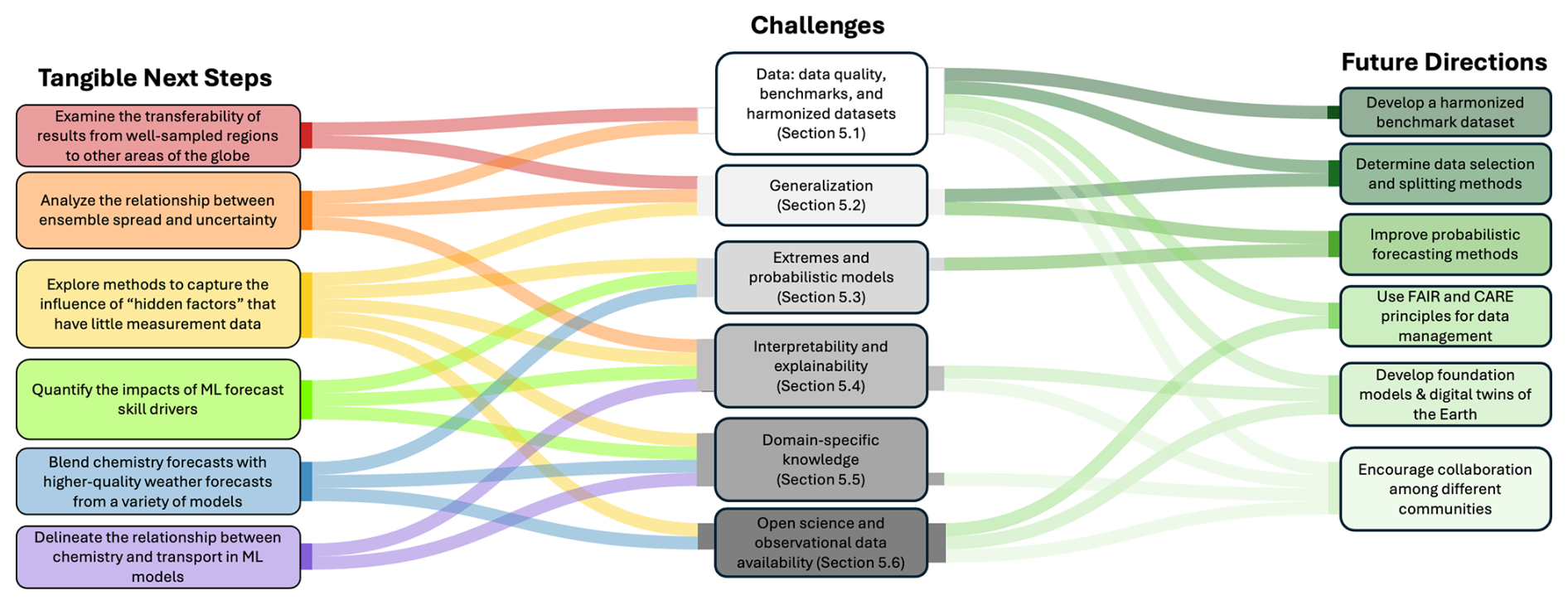
Figure 4 Challenges and future directions described in Sects. 5–6. The middle column represents the categories of challenges described in further detail in the sections listed. The left column lists specific projects that could be undertaken to address the challenges. The right column represents general future directions for the ozone AI/ML modeling community to consider. The lines connect categories of challenges with specific future directions and tasks that could address and resolve those challenges.

5.1 The challenges of data availability and workflow

Central to the success of ML modeling efforts and their utility are the choice of datasets and workflows, i.e., ML model choice and training methods. As noted above, in the field of air pollution and atmospheric composition research, the use of ML is hampered by the absence of benchmark datasets suitable for training different model types with varying sizes and complexity. Such well-defined benchmarks including datasets, training objectives, evaluation scores, and baseline models have been instrumental for the rapid development of ML models in other fields (Dueben et al., 2022). In particular, WeatherBench and WeatherBench2 (Rasp et al., 2020, 2024) have been key factors driving the transformation of ML weather forecasting between 2022 and 2024. A similar dataset to perform the same function for ozone forecasting would allow the robust comparison of different methods, and may guide the field towards more accurate models. Careful curation and data fusion of the TOAR surface ozone database with other relevant datasets might provide a robust and representative benchmark dataset, building on existing work (Betancourt et al., 2021). Ultimately, a lack of sufficient surface observations will impact the study of air quality and downstream impacts on health or vegetation. Therefore improving data coverage over poorly monitored areas remains a priority (Schultz et al., 2017).

The breadth of information available in datasets like TOAR, GHOST and reanalysis products like Copernicus Atmosphere Monitoring Service (CAMS) is vast, but these products provide significant challenges to the development of ML models for ozone due to heterogeneous data formats and lack of succinct documentation that focuses on the use of such data for ML applications. It may be that ML methods can also be used for infilling missing data (e.g. cloud-filtered satellite data, gaps in in-situ observations) for meteorological variables (Li et al., 2023) and ozone (Arroyo et al., 2018; Betancourt et al., 2022). Overall, there is a clear need for a harmonized benchmark dataset(s) for ozone to further enable ML models to be developed. These should (as much as possible) follow the vision outlined by Ebert-Uphoff et al. (2017) and the principles defined by Dueben et al. (2022).

With regards to model choice and development, it is worth noting that, in contrast to CTMs and other methods of simulation, ML models do not a priori require simulation, outputting and aggregating of high-resolution time series data to generate predictions for relevant ozone metrics. Instead, ML models can be trained to directly generate forecasts of these metrics (see Sect. 2). In this regard, it is necessary that ozone ML benchmarks should, where appropriate, include target objectives both for forecasting concentrations and for forecasting (a set of) aggregate ozone metrics. See Fleming et al. (2018) and Lefohn et al. (2018) for a more detailed discussion on relevant ozone metrics.

With regard to ML model training, there is a wide array of data-splitting approaches that can answer subtly related scientific questions. For forecasting it is common practice to divide the data temporally such that the training data completely precedes the testing data, such as using the last few years of a longitudinal dataset for testing. This is commonly recommended in benchmarking studies (Lam et al., 2023; Rasp et al., 2020). We emphasize that while these procedures likely make intuitive sense, they do not match the default setting in ML packages (Schultz et al., 2021), such as scikit-learn (Pedregosa et al., 2011), where the default cross-validation procedure will randomly split over individual data instances rather than over spatial blocks or temporal blocks. Without using these correct procedures, performance will be overestimated and may not reflect real performance when deployed. In practice, it remains a challenge to carefully define and document the data selection and splitting procedures and adapt them to the scientific problem at hand.

These challenges of data selection and splitting become particularly relevant when looking into climate timescales. Not only can this cause out-of-distribution samples of model input data (for example higher temperatures), but climate change may also affect atmospheric chemical and physical processes so that the mapping between inputs and outputs may drift. This problem is known as “concept drift”, where ML predictions become less accurate over time, which can arise from a non-representative training dataset or an ML model that lacks expressiveness, for example by being unable to extrapolate effectively beyond the bounds of the training data. For the latter, tree-based ML models especially are poor with respect to extremes and outliers. Here, model architecture may play a role. Exploring generative AI models, such as Generative Adversarial Networks (GANs) and transformer models, holds promise for the next generation of ML-based atmospheric models. These newer ML architectures can generate more internally consistent dynamics and require less training data than classical CNNs, while also demonstrating improved accuracy and stability over time.

5.2 The challenge of generalization

In addition to appropriate handling of training data, ensuring the trained model is as generally useful as possible, both in and out of sample, remains an enduring challenge. As is common in ML tasks, models trained on data from one geographical region may not necessarily transfer to another region, even when the underlying task and physics remain the same. This limitation often arises from variations in spurious features or unobserved variables specific to each domain, or differences in emissions and climate in different regions. Many approaches in the ML literature seek to improve the performance of ML models across domains, or under domain shifts, which are yet to be used for ozone forecasting (Sagawa et al., 2019), while recent studies suggest that large-scale weather forecasting models may generalize to unseen conditions and perturbations (Hakim and Masanam, 2024). generalization is particularly important for the use of ML models trained in high-data domains and then deployed in low-data domains. In this context, it may be useful to exploit the benefits of probabilistic forecasting (see following section), using models that report uncertainty in unfamiliar domains.

In the context of observational data, ML is increasingly used to derive or enhance geophysical variables from satellite measurements (see Sect. 4). However, a conceptual and practical challenge lies in the appropriate application of these ML-derived products across spatio-temporal scales (Di et al., 2017; Zhu et al., 2022; Tu et al., 2023) or atmospheric regimes (Ghahremanloo et al., 2023). There is a need to evaluate and document the scale-dependence of such products, and to guide their use in downstream modeling and analysis applications accordingly.

5.3 The challenges of extremes and probabilistic models

A relevant application for ozone forecasting and modeling is the study of extremes, including both accurate forecasting and attribution. Extreme ozone concentrations or fluxes can have a large impact on health and vegetation, and are also referred to as low-likelihood high-impact events. By definition, extreme events occur rarely and are hence challenging to accurately represent. There has been some work on approaches to weight extremes more during model training (Steininger et al., 2021). The ability of models to represent extremes is also an important metric that can be used to evaluate the quality of these models. Extremes can thus play a role for uncertainty quantification of the predictive performance of the models (e.g., important for forecast emulators and assessing ML performance on the extremes), where one can distinguish between epistemic (systematic) and aleatoric (statistical) performance. This connects with an increasingly recognized need to evaluate performance in more rigorous and consistent ways: including the development of new benchmark datasets, diagnostics, and metrics (see above). Progress on ML evaluation include causal evaluation (process-oriented approach) and eXplainable AI (xAI), for understanding (in)consistencies of the ML algorithms with physical processes (in other words: whether accurate answers are found for the right reasons). However, such methods are generally only applicable to relatively small-scale ML models. Dynamical tests and counterfactual experiments provide a means to test the credibility of large ML models (Hakim and Masanam, 2024; Baño-Medina et al., 2024).

Forecasting of potential extreme events is particularly challenging because these events are beyond the typical ozone variability, and naturally, extreme events are rarely and infrequently represented in data. For data-driven models this challenge is further exacerbated by (1) the need to forecast not only the presence of threshold exceedances, but also the intensity and duration of extreme events; and (2) ozone extreme events are often related to other anomalous mechanisms, such as heatwaves and wildfires, which are difficult to take into account based on limited extreme information, also due to the fact that ozone responses to these mechanisms are heterogeneous. Although the extreme value theory is widely adopted, its limitations are frequently acknowledged, including the IID (independent and identically distributed) assumption and independence between extreme and non-extreme events. On the other hand, approaches based on probabilistic forecasting may better characterize the uncertainty and likelihood of extreme events. One solution may be to use metrics and data scenarios to evaluate performance under different types of evaluation scenarios, taking advantage of evaluation metrics in weather forecasting which have been studied extensively. For example, if a key consideration is the ability of a forecasting model to capture extreme events, then metrics that capture relevant performance explicitly on those events should be used. This allows for robust comparison of both the existing and novel models on both traditional metrics and metrics focused on extreme event prediction to more comprehensively evaluate model performance. Evaluation of extreme events is limited in the literature, with recent studies highlighting the lower accuracy of ML models when forecasting spring and summertime ozone concentrations (Leufen et al., 2023; Hickman et al., 2023). In addition to helping with forecasting extreme events, probabilistic forecasting more generally provides a number of advantages compared to the deterministic forecasting methods that are currently more common, as outlined in Bodnar et al. (2024). Furthermore, ML weather forecasting models are increasingly adopting probabilistic and diffusion-based architectures that are able to produce sharp forecasts and uncertainty estimates. This is a promising line of work, however, these ML architectures may be challenging to implement for ozone forecasts due to the uncertainty driven by the meteorological fields themselves.

5.4 The challenge of interpretability and explainability

Interpreting and explaining ML models used to study ozone remains difficult. While these two terms are often used interchangeably, for this article we follow the distinction that interpretability focuses on designing and exploring models that are transparent and have comprehensible internal data transformations, whereas explainability methods focus on post-hoc explanations of how black-box models are working (Rudin, 2019). Models that are directly and trivially interpretable, such as multiple linear regression, are typically not the most performant, and in the high-data regime, the most performant ML models are typically variants on deep NNs that are difficult to interpret or explain. There is some literature that explores whether PINNs provide more interpretability. For example, efforts are underway to enhance the interpretability of ML models in atmospheric sciences by incorporating or diagnosing conservation priorities such as mass and stoichiometry (Sturm and Wexler, 2020, 2022). Additionally, neural operators are being employed to learn the solution operators of ODEs/PDEs from the chemical training data (Liu et al., 2024). However, while incorporating chemistry and physics constraints has been shown to increase interpretability, there is no guarantee that these methods will improve the stability of the ML model over time (Sturm et al., 2023). Often, there is a trade-off between interpretability and ML model accuracy, especially with more complex models (Sengupta et al., 2023). While methods to interpret and explain NNs more generally have been studied widely, mechanistic interpretability of NNs is a challenging task (Nanda et al., 2023), and only a limited range of XAI methods have been tested with ML methods developed for ozone forecasting, often focused on sensitivity approaches which look at the post-hoc explanations where the inputs to models are perturbed to see how predictions change (Ivanovs et al., 2021). Recent studies have investigated the importance of model input parameters through bootstrapping, i.e. random perturbations of individual inputs (Kleinert et al., 2021). Input data perturbation experiments are also possible and informative for very large models as, for example, demonstrated by Hakim and Masanam (2024) for the Pangu-Weather forecast model. Furthermore, ML approaches are increasingly employed to develop end-to-end models that process raw input data (e.g., emissions, meteorological fields) and directly predict outputs such as ozone concentrations. While end-to-end models bypass the challenges of emulating individual components, which are less prone to short-term instabilities and operator splitting issues, they also limit the ability to track uncertainty metrics tied to physical parameters and processes.

5.5 The challenges arising from domain-specific knowledge

Modeling ozone using ML proves challenging due to the multitude of sources driving model error (emissions, chemistry, transport, deposition) and the nonlinear response of ozone to these sources. Parameter tuning an appropriate ozone ML model for a complex, high-dimensional parameter space is possible given large computational resources and adaptive learning on pre-defined metrics. However, such an approach is largely inefficient given that atmospheric chemistry data lies on relatively low-dimensional manifolds with respect to the possible input parameter space. That is, many ozone-related relationships are structured with individual signals often being sparse and low-rank. Here, domain knowledge from atmospheric chemistry can help identify the optimal training dataset and define meaningful loss functions and targeted timescales (Fig. 1) for the ML model problem. In particular, domain knowledge of chemical and physical processes can help explain errors in ML models at short time scales versus long time scales. For example, ML models of atmospheric chemistry tend to predict well fast chemical processes (e.g., seconds to days) but diverge over longer time scales (e.g., months to years) (Kelp et al., 2020). In addition, knowledge of slow chemical processes, such as the role of peroxyacetyl nitrate (PAN) decomposition for ozone formation over polluted and/or remote areas, may help define appropriate training targets for ML models. An emphasis should be placed on emulating chemistry on longer timescales (>1 year) as issues of long-range stability are more challenging than shorter-term accuracy, and are a necessity for inclusion into CCMs and ESMs.

On the other hand, a heightened focus on domain knowledge may unintentionally limit the potential of ML models. Atmospheric chemists typically leverage well-established relationships of the chemical system, such as NO_x-limited vs. VOC-limited regimes, which are easily uncovered by linear regression or principal component analysis. By invoking such a strong prior assumption, it may impose constraints that hinder an ML model's ability to learn more complex, non-obvious interactions within the data. This bias toward known relationships risks overlooking patterns that could be hidden in the chemical state space that may promote greater accuracy and stability over longer time scales. Striking a balance between leveraging domain expertise and allowing ML models the flexibility to explore complex dynamics is essential for advancing the predictive capability of ozone modeling.

5.6 The challenges of open science and observational data availability

Although an open data infrastructure such as the TOAR-II database gives the impression of low barriers to data access, this might in fact not be true for everyone. Poor internet connectivity from developing countries may limit researchers from retrieving data and subsequently running a computationally demanding model (Blanken et al., 2022; Dwivedi et al., 2022). Furthermore, not all possible data providers agree with sending their data to an open access database, which is one important factor that limits global coverage of surface measurement data. The increasing resolution of satellite products and models is often considered to be an improvement, but the larger data size can complicate the processing and analysis of data for some researchers (Jain et al., 2022). Some data services require a registration and compliance with data use policies, which could conflict with institutional policies of researchers or exacerbate language barriers that non-native English researchers can experience. Finally, whereas advanced APIs can be ideal for technically skilled researchers and allow for reproducible workflows, they might hinder less technical researchers or policy makers that want to explore data sets.

In particular to developing nations, which may not have the economic ability to acquire high-resolution satellite products outside of those freely-available, it is imperative to develop high-quality, globally generalizable solutions to ozone modeling. Data hosting platforms like Google Earth Engine (GEE) enable users to freely access global data relevant for ozone modeling studies, ranging from land-use information from MODIS (Friedl, 2021) to human modification data from VIIRS nighttime lights (Elvidge et al., 2017), Gridded Population of the World (CIESIN, 2018), and more. Recent work by Kazemi Garajeh et al. (2023) investigated the ability to detect spatially resolved ozone pollution trends using time-series Sentinel-5 imagery from GEE, highlighting the quality of spatial distribution and accuracy available an open-source product and platform. This demonstrates the necessity to co-design data services and their hosting platforms to provide efficient and performant access to high-quality, well-documented data.

6 Future Directions

While new developments have been made in DL to utilize the expansive Earth observation data now available (Eyring et al., 2024), challenges remain regarding the quality, interpretability, and complexity of available data. Also, less work has been done to exploit atmospheric composition datasets, where observations are often less dense and more noisy than weather data. Future research and advancements in observational products suitable for ML, including efforts to address uncertainty quantification (e.g., Haynes et al., 2023), will enhance our understanding, facilitate process-based model evaluation (Nowack et al., 2020), and enable actionable science. Accurate forecasts of extrema in short-term surface ozone predictions are essential for protecting human health, while reliable projections of long-term changes in tropospheric ozone abundances are critical for understanding climate change and its impacts. Leveraging causal- and physics-constrained data-driven approaches can enhance trust and interpretability in ML-based modeling efforts (Tesch et al., 2023; Beucler et al., 2024), and combining causal discovery and xAI methods holds potential for advanced process-based evaluation (Iglesias-Suarez et al., 2024). There is a recognized need to evaluate model performance rigorously and consistently, calling for the development of new benchmark datasets, diagnostics, and metrics (Betancourt et al., 2021, 2022), to enable comprehensive evaluation of ML-based ozone modeling techniques. To meet society's needs facing current environmental challenges by providing actionable science and maintaining rapid progress in this field, collaboration among atmospheric composition communities and ML communities is essential.

To thrive, the interdisciplinary ozone modeling and forecasting community requires open knowledge sharing, resources and research cooperation. Research in the domain should adhere to the FAIR principles of Findability, Accessibility, Interoperability and Reusability (Wilkinson et al., 2008) and the CARE principles of Collective, Authority to control, Responsibility and Ethics (Carroll et al., 2021). Availability of data is essential for data-driven approaches and the developed TOAR-II surface ozone database is essential here through its open data policies and its Application Programming Interface (API), which allow for automatic extraction of data.

Future work may focus on foundation models to advance more integrated approaches. These models, trained on extensive datasets in a self-supervised manner Bommasani et al. (2021), have already demonstrated their capability in fields like weather forecasting and climate science (Lessig et al., 2023; Nguyen et al., 2023; Bodnar et al., 2024). In the context of tropospheric ozone modeling, foundation models could improve performance by learning from varied datasets, including observational and numerical modeling data (Mukkavilli et al., 2023). These models are capable of handling multiple air pollutants simultaneously and can incorporate meteorological variables, supporting the development of more comprehensive, flexible and potentially robust air quality benchmarks by harmonizing observational data. Their flexible architectures enable training a single model with large-scale resources and then fine-tuning it for multiple tasks, reducing the computational expense of repeated model training (Bommasani et al., 2021).

At present, there are underexplored opportunities to merge the current successes in ML weather and climate model emulation with CTMs and ESMs. Thus far, atmospheric chemistry data have been largely excluded from ML weather and climate applications, as these current supervised learning frameworks are typically non-extensible, requiring retraining of the entire ML model when incorporating new chemical information. In contrast, unsupervised learning model frameworks, such as pre-trained foundation models, can identify patterns in data without explicit labels, offering a new frontier for ingesting and potentially improving ML modeling of atmospheric chemistry. These foundation models can be fine-tuned on CTM data. For example, the Aurora model (Bodnar et al., 2024) is fine-tuned on a subset of six criteria pollutants, including ozone from CAMS (Inness et al., 2019). Fine-tuning ML weather and climate models enables the addition of chemical species to an ML model that is already trained on atmospheric dynamics. This process of fine-tuning, by training specific decoders for new variables, has also recently been carried out for hydrological variables (Lehmann et al., 2025). However, adding chemical species such as VOCs in the absence of emission inputs (which current models do not consider) on the ML weather model's native 6 h forecast time steps likely presents challenges. Greater emphasis is needed on understanding the factors influencing ML model performance with respect to the specific challenges of atmospheric composition research and air quality analysis.

While much progress will likely be made by large coordinated efforts to build comprehensive datasets and foundation models (or fine-tune existing foundation models), progress on important problems specific to ozone may be achieved without requiring large-scale, compute-intensive projects (see Fig. 4). First, investigation of the influence of sparsely observed factors on the skill of ozone forecasting models would be useful. For example, VOCs are not widely measured, and the impact of including VOCs as inputs to an ozone forecasting model could be explored. Second, the capacity of models to predict ozone formation in under-observed regions, after being trained on well-sampled regions, may also provide information about the generalizability of ML models. This work could also inform the importance of largely unobserved variables that influence ozone but differ between regions. More generally, a systematic exploration of the factors that influence machine learning model skill in modeling ozone would be useful for the field. In addition, since much data for model training comes from CTMs, which often have degraded resolution compared to the most accurate weather models, improved model accuracy may be obtained by combining high resolution weather models with chemistry data from lower resolution models. This relates to delineating chemistry and transport in models. Since ML models do not explicitly transport chemical tracers, it may be interesting to explore how ML models perform for tracers with different lifetimes. Furthermore, as probabilistic machine learning methods are established for ozone modeling, analyzing the relationship between ensemble spread and ensemble error could be insightful.

7 Conclusions

While modeling ozone accurately remains a challenging problem across temporal and spatial scales, ML approaches have made progress in a number of areas. As highlighted in this Perspective, ML methods are contributing to research in short-term forecasting, chemistry model emulation, and remote sensing of ozone. Specifically, ML methods are providing increasingly accurate short-term forecasts of ozone at observational stations, and making progress toward providing fast emulators of chemical mechanisms used in chemistry-climate models. In remote sensing, ML methods have shown skill in increasing the efficiency of ozone retrieval, and in making estimates of ozone where there is little satellite coverage.

Similar to many applications of ML to physical modeling, for our field to make progress in modeling real-world ozone faithfully, models should be trained with a synthesis of high-quality observational datasets and appropriate high-quality benchmarks must be compiled to evaluate the skill of different models, and enable the comparison of ML and numerical models. Furthermore, continued work to mitigate the ozone-specific challenges faced by existing ML models is necessary, as highlighted in Sect. 6, which will require close collaboration between domain experts and ML researchers to develop models tailored to the particular challenges. Notably for ozone modeling, recent work illustrates that foundation models, trained on diverse datasets, are capable of skillful atmospheric composition modeling. The paradigm of foundation models represents a significant step forward for composition modeling, enabling an integrated approach across multiple scales and tasks, and building on the success of similar models for weather forecasting. However, it remains an open and important question whether ML models can contribute to improved process-level understanding of drivers of ozone, including quantifying the influence of sparsely observed drivers, and generalize to unseen air pollution and climate scenarios.

As ML continues to transform ozone research and adjacent fields, including weather and climate modeling, the ozone modeling community needs to ensure future research builds on strong foundations. By developing robust benchmarks, building productive cross-disciplinary collaborations, and embracing state-of-the-art techniques, ML-driven ozone research has the potential to not only advance scientific understanding but also deliver actionable benefits for climate resilience and public health.

Appendix A: Glossary

Glossary of terms and abbreviations
Artificial Intelligence (AI)	A software or model that is capable of performing tasks that typically require human intelligence.
Copernicus Atmosphere Monitoring Service (CAMS)	A service by the EU Earth observation programme to provide comprehensive data on atmospheric composition and air quality through satellite and ground-based monitoring.
Chemistry-Climate Model (CCM)	A type of global model focused on the interactions between atmospheric chemistry and climate.
Convolutional Neural Network (CNN)	A type of neural network designed for processing data with grid structure, often used for image processing.
Chemical Transport Model (CTM)	A type of global model designed to simulate the movement and chemical reactions of atmospheric pollutants.
Deep Forest (DF)	A deep learning architecture based on decision trees instead of neural networks.
Deep Learning (DL)	A field of machine learning focused on the development and use of neural networks.
Decision Tree (DT)	A hierarchical supervised learning algorithm, often used to create classification and regression models.
Earth System Model (ESM)	A global model that simulates all aspects of the Earth system, including the interactions between the atmosphere, oceans, land, and biosphere.
Feed-forward Neural Network (FNN)	A basic type of neural network where data move in one direction without feedback loops, often used for data classification and recognition.
Foundation Model (FM)	A machine learning model trained on vast amounts of data, designed to be adapted to a broad range of tasks.
Generative Adversarial Network (GAN)	A type of machine learning technique where two neural networks compete unsupervised to produce the most accurate result.
General Circulation Model (GCM)	A global model that simulates the Earth’s atmospheric dynamics and circulation.
Gradient Boosted Decision Tree (GBDT)	An ensemble machine learning technique that uses the results of multiple decision trees to improve accuracy and reduce error of the prediction.
Large Language Model (LLM)	A type of foundation model trained on very large text datasets to understand and generate natural language.
Long Short-Term Memory network (LSTM)	A type of recurrent neural network designed to retain information over longer sequences for longer periods.
Machine Learning (ML)	A field of artificial intelligence dedicated to algorithms and models that can learn and make predictions from the input data without being explicitly programmed to do so.
Neural Network (NN)	A machine learning model designed to process data in a similar way as the human brain.
Physics-Informed Neural Network (PINN)	A type of neural network trained to follow known physical laws.
Random Forest (RF)	An ensemble machine learning algorithm that combines multiple decision trees during the training process to improve prediction accuracy and reduce overfitting.
Recurrent Neural Networks (RNN)	A type of neural network in which data can loop back into the network retaining memory of previous inputs. It is designed for sequential data processing where context is important, such as natural language and time series.
Transformer Model (TM)	A type of deep learning model that converts a given input into a desired output, learning context and meaning. It is used as a foundation model for large language models as an alternative to CNNs and RNNs architectures.
U-Net	A type of convolutional neural network designed for image segmentation and de-noising.
eXplainable AI (xAI)	A type of artificial intelligence that provides the information necessary to understand how a certain output was achieved.