A computationally efficient method to model similar and alternate stratospheric aerosol injection experiments using prescribed aerosols in a lower-complexity version of the same model: a case study using CESM(CAM) and CESM(WACCM)

Climate model simulations incorporating stratospheric aerosol injection (SAI) generally require more computational resources compared to out-of-the-box applications, due to the importance of stratospheric chemistry. This presents a challenge for SAI research, especially because there are numerous ways and scenarios through which SAI can be implemented. Here, we propose a novel application of pattern-scaling techniques that allows us to generate SAI forcing in the Community Atmosphere Model (CAM) – a model without interactive stratospheric chemistry – using pre-existing data from the Whole Atmosphere Community Climate Model (WACCM), a state-of-the-art model with interactive stratospheric chemistry, but expensive to run. In doing so, a significant portion of the computational budget is saved. The present method requires a pre-existing dataset of a representative SAI experiment and its corresponding control experiment, with interactive stratospheric chemistry. The data is converted into a set of relations to determine the forcing fields given any required optical depth of the aerosol field. The present method is suitable for applications that use dynamical feedback controllers and is intended to aid impact research into the tropospheric and (sub)surface climate changes due to SAI. The results of climate simulations with aerosols prescribed by the present procedure are in close agreement with those from the full-complexity model, even for different model versions, horizontal resolutions and SAI forcing scenarios.

1 Introduction

Each of the past ten years (2015–2024) was individually among the ten warmest years on record, with global mean surface temperature (GMST) in 2024 reaching 1.55 °C above pre-industrial levels (World Meteorological Organization, 2025). The recent warming trend raises concerns about potentially exceeding temperature thresholds for several climate tipping points (McKay et al., 2022). Solar Radiation Modification (SRM) – measures to directly influence the earth's radiative balance (National Academies of Sciences and Medicine, 2021) – has been suggested as potential auxiliary measure to reduce global warming and, potentially, tipping risks (Futerman et al., 2025; Hirasawa et al., 2023). One such SRM method is Stratospheric Aerosol Injection (SAI), which involves the injection of sulfate aerosol (precursors) to form a reflective stratospheric aerosol layer.

Modelling SAI entails considerable computational costs, not least because of the great number of possible scenarios combining, for example, different starting times, intensity and location (mainly latitude and height) of interventions (Visioni et al., 2023; MacMartin et al., 2022; Visioni et al., 2023). Not only would a high number of model years be needed to sample the scenario space with Earth System Model (ESM) simulations, but also the computational costs per model year can be high for simulations including stratospheric chemistry and aerosol processes. For example, the CESM2(WACCM6) (Gettelman et al., 2019), which has been used for many SAI simulations (e.g. Tilmes et al., 2018, 2020), is roughly seven times more expensive to run at 1° nominal resolution than the CESM2(CAM6), a model version without stratospheric chemistry and a lower model top (Danabasoglu et al., 2020). High costs of running stratospheric chemistry models may be one reason for the low number of high-resolution climate simulations with SAI so far. Higher resolutions are needed to resolve important weather phenomena such as tropical cyclones (Roberts et al., 2020) and can improve some, though not all, model biases (Jüling et al., 2021; van Westen and Dijkstra, 2021).

In this paper, we suggest a method to approximate SAI's climate impacts in CESM(CAM) rather than the full-complexity CESM(WACCM). The method is not suitable for studies focusing on stratospheric processes, but may be useful to save computation time when the focus is on tropospheric or oceanic impacts.

Multiple studies have developed the technique to prescribe stratospheric aerosol effects in climate models that do not simulate aerosols interactively. It has been used in models such as CNRM and MPI-ESM, which participated in G6sulfur (Visioni et al., 2021), and were driven by externally derived aerosol forcing datasets, for example from Tilmes et al. (2015) or similar internally generated and scaled datasets. A comparable approach has been used in CESM(CAM-chem) simulations (Xia et al., 2017), and in the CCMI SAI protocol (Tilmes et al., 2025), where forcing data are prescribed rather than interactively calculated. To maintain specified temperature targets, the aerosol optical depth (AOD) and aerosol mass are typically scaled linearly. For instance, Tilmes et al. (2022) report that linear scaling of forcing strength in the CNRM model led to linear increases in SAD due to fixed aerosol size, despite physical expectations of size variation with forcing strength (Niemeier et al., 2011; Niemeier and Timmreck, 2015).

For determining the aerosol fields, we make use of pattern-scaling techniques by projecting the (seasonally and spatially varying) fields onto a single reference variable, here global mean AOD. Pattern scaling has been used extensively for emulating climate responses (e.g. Lynch et al., 2017), including in SRM research (e.g. MacMartin and Kravitz, 2016; Muñoz-Sánchez et al., 2025; Farley et al., 2024). Often, linear relationships are assumed, although these may not work for some variables such as sea ice (MacMartin and Kravitz, 2016) or stratospheric ozone (MacMartin et al., 2019). In contrast, we do not assume linearity, but merely a monotonic dependence between the relevant stratospheric forcing fields and global mean AOD.

Directly inserting WACCM-derived aerosol fields into CAM can lead to problems, as both models show different Global Mean Surface Temperature (GMST) responses to the same amount of stratospheric aerosol forcing. This is particularly undesireable when working with SAI scenarios based on climate targets such as fixing GMST. We therefore make use of a proportional-integral (PI) feedback controller developed by MacMartin et al. (2014), Kravitz et al. (2016, 2017) and Tilmes et al. (2018) that regulates aerosol injection (at several latitudes) in order to achieve (multiple) specified temperature targets. While the feedback controller may operate independently, it is often paired with a prescribed feedforward estimate – an informed approximation of the necessary aerosol forcing – to enhance performance. Prominent examples include CESM(WACCM) simulations within the G6sulfur scenario (Visioni et al., 2021), GLENS (Kravitz et al., 2017), and the ARISE-SAI protocol (Richter et al., 2022), all of which incorporate such combined strategies. These experiments generally provide the most realistic climate response to SAI due to the active stratospheric chemistry at the cost of computational power.

We combine these prior strands of work into a procedure that allows us to easily automatize the scaling of the aerosol forcing and take into account non-linear relationships between relevant aerosol field, both of which has not been commonly done in prior studies prescribing aerosol forcing for SAI (e.g. Visioni et al., 2021; Xia et al., 2017; Tilmes et al., 2022).

In a nutshell, the procedure works as follows:

• Use the difference between a simulation with SAI and a control simulation without SAI in CESM(WACCM) to separate each forcing variable into a spatio-seasonal and an annually varying component.

• Relate the annual intensity for all forcing variables to that of the annual global mean stratospheric aerosol optical depth (n_AOD) using suitable fitting functions.

• During the simulation, annually determine the required n_AOD based on the past deviations of GMST from target temperature and translate into the forcing fields using the relations determined above.

To assess how well the procedure works, key climate variables (surface temperature, precipitation, zonal mean temperature and zonal mean wind) are inspected in a simulation with CESM(CAM) that aims to imitate the SAI forcing in the original multi-objective CESM(WACCM) simulation. We verify that GMST, the interhemispheric gradient and equator-to-pole gradient of surface temperature responses to SAI are similar in both models. The inter-model differences in response to SAI forcing are compared to their natural interannual variability through a performance index. To test for the transferability of the proposed method, we assess results from similar runs with a delayed SAI scenario, we implement a different model version with a differing initial climate state and aerosol representation, and explore the role of a higher spatial resolution.

In Sect. 2, an overview of the simulations is presented and the steps of our method are explained in more detail. In Sect. 3, our method is validated by comparing the climate responses to SAI in the WACCM and CAM simulations, and its transferability to an additional SAI scenario, differing initial state and higher model resolution is tested. This is followed by a discussion of the results and potential use cases in Sect. 4, conclusions in Sect. 5 and an outlook in Sect. 6.

2 Methods

2.1 Model and simulations

Our “working horse” model is CESM2, of which we use two configurations, namely CESM2(WACCM6) with interactive stratospheric aerosols and CESM2(CAM6) without. In addition, results using the older model version CESM1 (again with either WACCM or CAM) are briefly discussed, mainly to test the effect of model resolution. In both cases, we used existing WACCM simulations to extract aerosol fields, and used these to force CAM.

The CESM2(WACCM6) model (Gettelman et al., 2019) is run at a nominal horizontal resolution of 1° for atmosphere and ocean. WACCM6 has 70 vertical levels with a model top of $\mathrm{6}\times {\mathrm{10}}^{-\mathrm{6}}$ hPa (140 km). Aerosols are simulated using the 4-mode Modal Aerosol Module (MAM4), which includes relevant heterogeneous reactions on the aerosol surface. More details are provided by Liu et al. (2016).

The simulations with CESM2(WACCM6) (henceforth simply `CESM(WACCM)') consist of a control simulation with high greenhouse gas forcing, WACCM-Control (Danabasoglu, 2019), and a simulation with similar background forcing but applying SAI to counteract the warming pattern, WACCM-SAI2020 (see Fig. 1). Greenhouse gas concentrations and other anthropogenic forcings follow the SSP5-8.5 scenario in WACCM-Control. In WACCM-SAI2020 (Tilmes et al., 2020), the GMST target value is 1.5 °C above pre-industrial, which roughly coincides with 2020 values. SO₂ is injected at four latitudes to keep three target variables, GMST (T₀), the interhemispheric surface temperature gradient, T₁, and the equator-pole surface temperature gradient, T₂, at their [2015–2024] levels. More details on the feedback procedure and temperature targets are provided by Kravitz et al. (2017).

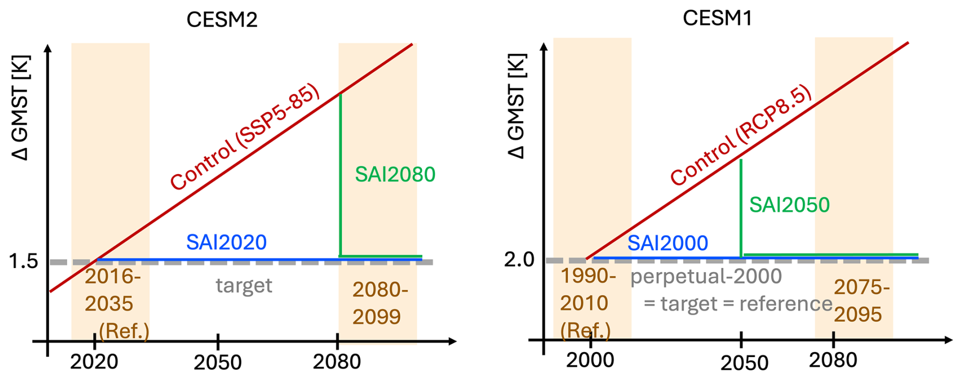
Figure 1 Schematic of scenarios used in CESM2 (left panel) and CESM1 (right panel). SAI2080 and SAI2050 are only run with CESM(CAM). Shaded areas denote periods used in Sect. 3, namely a present-day reference period and an end-of-century period. In the case of CESM1, the perpetual-year-2000 simulation is used as reference.

For the CESM2 simulations conducted in this study, CESM2.1.3(CAM6.0) (Danabasoglu et al., 2020) is used, henceforth simply “CESM(CAM)”. This model likewise uses the MAM4 aerosol scheme with interactive tropospheric chemistry and prescribed stratospheric aerosols (with three modes for sulphate aerosol, similar to WACCM). CESM(CAM) is run at a nominal resolution of 1° for the atmosphere and 1° for the ocean. CAM has 32 vertical levels and a model top at 3 hPa (40 km).

With CESM(CAM), we simulate the same scenarios as with CESM2(WACCM), ie. one control simulation (CAM-Control) without SAI, where anthropogenic forcing follows SSP5-8.5 until 2100 and stays constant thereafter, and one (CAM-SAI2020) in which SAI is used from 2020 onwards to keep GMST at present-day levels. An additional simulation, CAM-SAI2080, follows the control scenario until 2080, in which year SAI is started to reduce GMST to present-day levels (see Fig. 1). This simulation is used to test whether our method is able to model scenarios not previously modelled in CESM(WACCM).

In addition, simulations performed with CESM1.0.4(CAM5) (Hurrell et al., 2013) are briefly discussed, to explain slight adjustments to our method that are required for CESM versions that are forced with single-mode stratospheric aerosols and test the transferability of our method to higher model resolutions. In this model version, the aerosols are prescribed as volcanic aerosols with a fixed size distribution. The nominal horizontal resolution is 1° for the atmosphere and ocean. The control simulation follows the RCP8.5 (CO₂ only) scenario from 2000 to 2100 and is branched from an equilibrated spinup run with perpetual year-2000 conditions (van Westen et al., 2020). Two SAI experiments are branched from the control simulation: CAM5-SAI2000 (CAM5-SAI2050), starting SAI in 2000 (2050) to cool down to 2000 values of GMST. For CAM5, year-2000 conditions are defined as the [1990–2009] average of the spinup. Additionally, results with this model version are shown for a similar high resolution case having a nominal resolution of 0.5° for the atmosphere and 0.1° for the ocean. The aerosol forcing data are derived from CESM1(WACCM) simulations by Kravitz et al. (2017). These simulations start from a historic forcing scenario and are therefore slightly cooler than the CAM5 simulations.

An overview of the WACCM data used and simulations carried out in this study, is provided in Table 1. Code and data needed to reproduce the simulations in this study are provided by de Jong et al. (2025b).

Tilmes et al. (2020)Tilmes et al. (2020)Kravitz et al. (2017)Kravitz et al. (2017)

Table 1 Simulation overview.

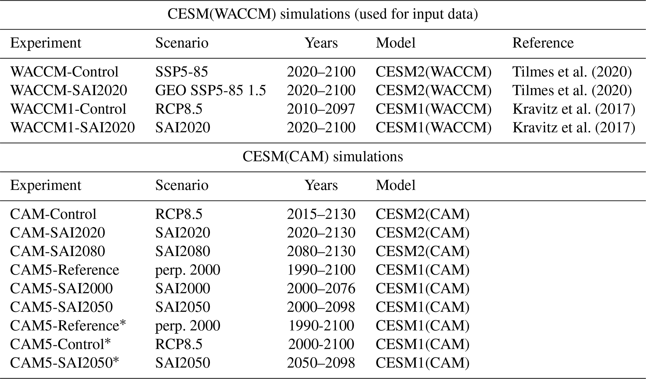
^* High-res: nominal resolution 0.5° atmosphere, 0.1° ocean.

In the results section, spatial maps generally represent the [2080–2099] SAI2020 average (late-century SAI2020) minus the [2016–2035] Control average (present-day). The latter period is longer than the period used to determine the target metrics in CESM(WACCM), such that anomalies with respect to present-day are more robust. In some spatial maps, the [2080–2099] Control average is used. We will simply refer to Reference (present-day Control), Control (late-century Control) and SAI (late-century SAI2020). While these words are also used to describe the simulations (e.g. CAM-Control), the meaning should be clear from their context. Similar definitions apply for CAM5, where Reference is the [1990–2009] average of the spinup and Control (SAI) the [2080–2099] period of CAM5-Control (CAM5-SAI2000).

2.2 Deriving aerosol forcing patterns

As briefly explained in the introduction, we use the outcome of CESM2(WACCM6) simulations with interactive stratospheric aerosols (Tilmes et al., 2020) as basis for prescribed stratospheric aerosol fields in CAM. Expanding on the work of Pflüger et al. (2024), we explain the four steps necessary to construct the prescribed stratospheric aerosol fields: pre-processing, normalization, averaging and scaling. The end result is a mapping from a user-specified SAI amplitude to appropriately scaled aerosol fields that still retain seasonal variations.

2.2.1 Pre-processing

The background signal that is present in the Control run of CESM2(WACCM6) is subtracted from the SAI2020 run. By doing this, we try to avoid a scaling of spurious aerosol contributions unrelated to SAI.

We write

$$F_i^{\mathrm{Diff}}(y,d,x)=F_i^{\mathrm{SAI}}(y,d,x)-F_i^{\mathrm{Control}}(y,d,x)$$

where F_i refers to a specific aerosol variable in either the SAI2020 ($F_i^{\mathrm{SAI}}$) or the Control run ($F_i^{\mathrm{Control}}$). The fields represent relevant stratospheric aerosol variables such as mass concentrations and wet diameters, see Table 2, and are defined for every year y, day of the year d and spatial coordinate x. Here, x can also refer to a set of coordinates, such as latitude and pressure level.

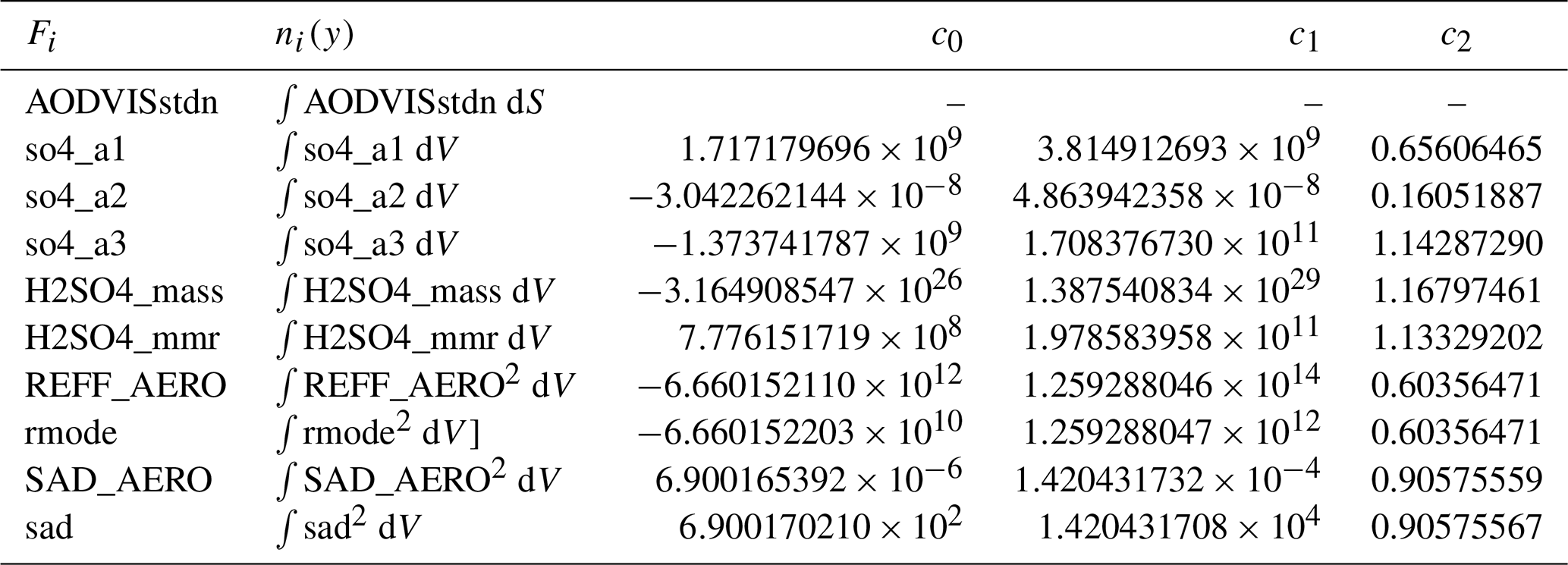
Table 2 Normalization of stratospheric aerosol fields in CESM2.

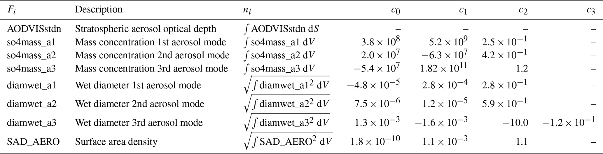
Aerosol fields, normalization scheme, fit parameters w.r.t. AOD; fitting functions found in text; ∫ … dS represents the annual mean global surface mean, ∫ … dV the annual mean volume integral over the entire atmosphere.

2.2.2 Normalization

All fields ΔF_i are normalized through field-specific, annual scale factors n_i(y). This step ensures that the interannual average of the normalized field (see below) is not dominated by years in which aerosol forcing is strong (in our case, the end of the simulation, as SAI injection rates increase over time).

The normalized fields are written as

$${\widehat{F}}_i(y,d,x)={\displaystyle \frac{F_i^{\mathrm{Diff}}(y,d,x)}{n_i\left(y\right)}}.$$

An example for scale factor n_i(y) would be the annual-mean total atmospheric mass – as obtained by spatial integration – derived from a mass concentration field. The choice of normalization is arbitrary to some extent, but should increase monotonically with the overall intensity of SAI as specified by the n_AOD. All fields and respective normalizations are listed in Table 2. For CESM1, these values are listed in Table C1.

2.2.3 Averaging

The normalized fields are averaged over a given time period, from an initial year y_i to a final year y_f. In our case, we choose y_i=2070 and y_f=2100, meaning that our aerosol fields are representative of relatively high aerosol burdens.

The averaged field becomes

$${\stackrel{\mathrm{‾}}{F}}_i(d,x)={\displaystyle \frac{\mathrm{1}}{y_{\mathrm{f}}-y_{\mathrm{i}}+\mathrm{1}}}\sum _{y=y_{\mathrm{i}}}^{y_{\mathrm{f}}}{\widehat{F}}_i(y,d,x).$$

In the process of averaging, the fields lose their interannual but not seasonal variability.

2.2.4 Scaling

The scale factors n_i(y) from all fields except AOD will now be expressed in terms of n_AOD. This is where the choice of normalization scheme becomes relevant. We see in Fig. 2 how the scale factors n_i(y) relate to n_AOD(y) in any given year y, and how these relationships are roughly monotonic. With that, it is reasonable to perform fits that map a given n_AOD onto a respective value $n_i^{\mathrm{fit}}$.

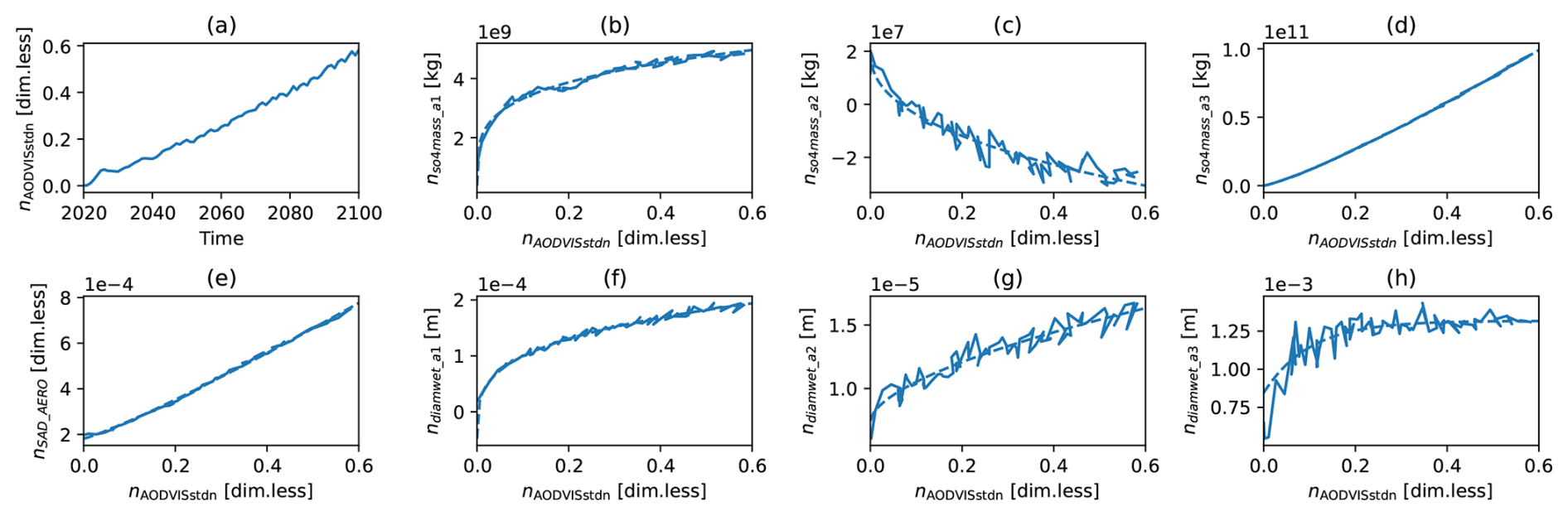
Figure 2 Scale factors of stratospheric aerosol fields derived from WACCM-SAI2020 minus WACCM-Control. (a) n_AOD against time, (b–h) n_i of remaining fields (cf. Table 2) against n_AOD (solid) and their fits $n_i^{\mathrm{fit}}$ (dashed).

For most variables, a power-law relationship yields good fits:

$$n_i^{\mathrm{fit}}\left(n_{\mathrm{AOD}}\right)=c_{\mathrm{0}}+c_{\mathrm{1}}{n}_{\mathrm{AOD}}^{c_{\mathrm{2}}}.$$

For the variable diamwet_a3, a (saturating, c₂<0) exponential function yields a better fit:

$$n_{\mathrm{dw}\mathrm{3}}^{\mathrm{fit}}\left(n_{\mathrm{AOD}}\right)=c_{\mathrm{0}}+c_{\mathrm{1}}\exp \left(c_{\mathrm{2}}\left(n_{\mathrm{AOD}}-c_{\mathrm{3}}\right)\right).$$

As soon as we specify a timeseries, n_AOD(y), e.g. by the feedback–feedforward controller seen in the next section, we can obtain the final prescribed fields for CAM

$$\begin{array}{}\text{(1)}& F_i(y,d,x)=n_i^{\mathrm{fit}}\left(n_{\mathrm{AOD}}\left(y\right)\right){\stackrel{\mathrm{‾}}{F}}_i(d,x).\end{array}$$

Of course, in the case of the AOD field, n_AOD(y) can be used directly without any fit.

For any desired value of n_AOD, the above procedure essentially generates the expected WACCM output for a year in which the global mean stratospheric aerosol optical depth in WACCM is equal to n_AOD. Here we assume that the changes in e.g. particle size and aerosol mass respond fast to changes in n_AOD. Slow dynamical responses, e.g. triggered by changing sea surface temperature, may therefore cause some discrepancies and will be investigated in the validation (Sect. 3). In practice, adjusting the n_AOD using a feedback controller is a robust approach of dealing with these discrepancies, though it may resolve only large-scale pattern differences (MacMartin et al., 2014).

2.3 Feedback–feedforward control algorithm

By dynamically adjusting the SAI intensity in the form of n_AOD, we can stabilize the GMST (T₀), to a predefined target temperature, T_0,target. We do this by adapting a feedback–feedforward control scheme (MacMartin et al., 2014; Kravitz et al., 2016, 2017; Tilmes et al., 2020) which observes the temperature error $\mathrm{\Delta }{T}_{\mathrm{0}}\left(y\right)=T_{\mathrm{0}}\left(y\right)-T_{\mathrm{0},\mathrm{target}}\left(y\right)$ and dynamically constructs an SAI intensity n_AOD(y) that is supposed to minimize ΔT₀(y).

The control scheme is a sum of three terms, the proportional and integral feedback components which follow the current and historical temperature error respectively, and a feedforward term that increases linearly in time (Pflüger et al., 2024)

$$n_{\mathrm{AOD}}\left(y\right)=\underset{\mathrm{feedforward}}{\underbrace{k_{\mathrm{ff}}\left(y-y_{\mathrm{0}}\right)}}+\underset{\mathrm{proportional}}{\underbrace{k_p\mathrm{\Delta }T\left(y\right)}}+\underset{\mathrm{integrator}}{\underbrace{k_i\sum _{y^{\prime }=y_{\mathrm{i}}}^y\mathrm{\Delta }T\left(y\right)}}.$$

Here, k_ff, k_p, k_i are pre-defined parameters regulating the strength of feedforward and feedback, y₀ specifies the onset of the feedforward for y>y₀ and y_i is the onset year for the integrator. The feedforward is a first guess of the strength of the aerosol forcing field needed to reach the GMST target. Improving the feedforward may enhance the performance of the feedback–feedforward controller, though a perfect estimate is not needed. In CESM1 we found that applying a feedforward that was about twice as strong as needed only resulted in a moderate overcooling of 0.2 °C (not shown). If a better feedforward is desired, one can fine-tune its scale factors values after a test simulation as shown below.

Note that the form above is just one possible implementation of a feedback–feedforward controller tailored to our case. Depending on the underlying GHG forcing scenario, it could also make sense to have a feedforward that changes non-linearly in time. In fact, we modify the formula above whenever we perform post-21st century simulation with stabilized GHG levels after 2100. In that case, the feedforward is kept constant after 2100. Parameter values are given in Table 3.

Table 3 Feedback–feedforward parameters of CAM-SAI simulations.

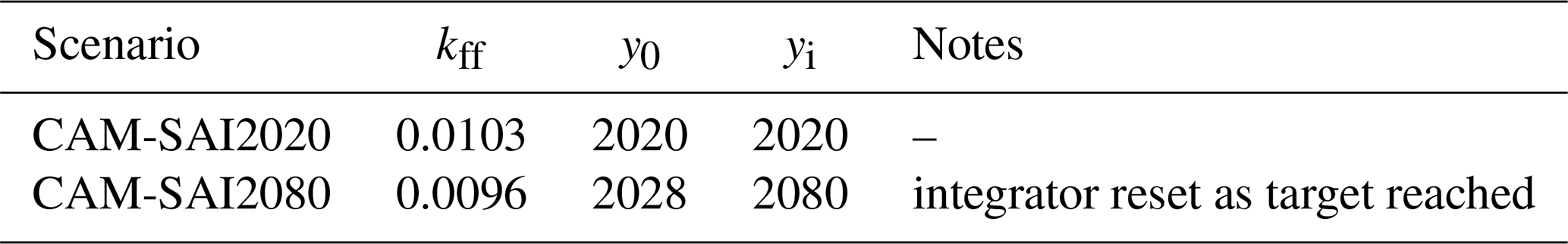
In both cases k_i=0.028 and k_p=0.028 following a previous CESM2 study (Tilmes et al., 2020). The scenarios branch off CAM-Control in 2020 and 2100 respectively and have capped feedforwards after 2100.

We implement one significant modification to the above procedure in the case of the CAM-SAI2080 scenario, the physical extreme scenario of rapid cooling in a late-century hot climate. If the integrator were activated right at deployment in 2080, it would accumulate large temperature errors which prompt an overcooling. If instead the integrator were not activated, convergence to target temperature may be too sluggish. Hence, we activate the integrator at the start of the deployment but reset the sum of errors after roughly six years when the target temperature is reached. That way, we achieve quick convergence with limited overcooling (Fig. 3b).

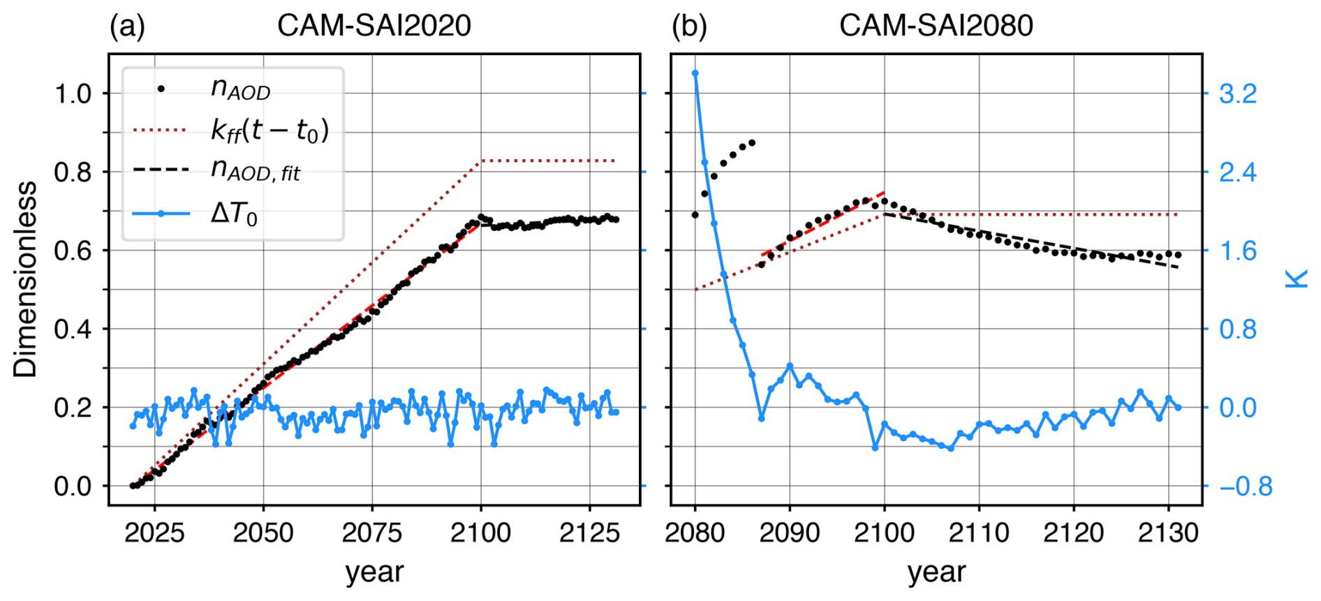
Figure 3 n_AOD and GMST error. Black dots indicate the n_AOD applied to the simulation, dotted lines show the feedforward component hereof. Dashed lines show the best piecewise linear n_AOD fit after run completion. In blue, the GMST error w.r.t. the target temperature is shown.

Feedback–feedforward controller results for CAM-SAI2020 and CAM-SAI2080 are shown in Fig. 3. In CAM-SAI2020, the GMST error from target, ΔT₀, is close to zero. The actual forcing, which is the sum of the feedforward and adjustment based on the (history of) ΔT₀, is about 20 % weaker than the feedforward, i.e. the feedforward is slightly too strong. In CAM-SAI2080, the initial ΔT₀ is quite large. After seven years of strong cooling, the target temperature has been reached and the sum of temperature errors is reset to zero, causing a sudden drop in n_AOD. After this, ΔT₀ is roughly zero with a maximum error of 0.4 °C. Preliminary tests with the feedback-feedforward controller using a climate emulator (Millar et al., 2017) with random noise to simulate the GMST response showed that adjusting the gains of the controller may reduce, but not eliminate, the temperature undershoot.

Optimized values of the feedforward constants may be obtained from fitting the applied n_AOD. Dashed lines in Fig. 3 indicate such linear fits, showing in hindsight what would have been the optimal values for k_ff, y₀ (and maximum feedforward strength after 2100). In this case, the AOD increase of about 0.68 in 80 years corresponds to an optimal value for k_ff of 0.0085. The feedback controller code and analysis to derive the aerosol forcing patterns are provided by de Jong et al. (2025a).

2.4 Performance index

We define the following index to measure the similarity in SAI response (SAI minus Reference) between CAM and WACCM:

$$\begin{array}{}\text{(2)}& {\displaystyle \frac{\left({\mathit{\mu }}_{\mathrm{CS}}-{\mathit{\mu }}_{\mathrm{CR}}\right)-\left({\mathit{\mu }}_{\mathrm{WS}}-{\mathit{\mu }}_{\mathrm{WR}}\right)}{\sqrt{s_{\mathrm{CR}}^{\mathrm{2}}+s_{\mathrm{WR}}^{\mathrm{2}}}}},\end{array}$$

where μ and s are the interannual mean and standard deviation, respectively. In subscripts, “C” or “W” means CAM or WACCM, and “S” or “R” means SAI2020 or Reference, respectively, as defined in Fig. 1. The denominator of this expression represents the interannual standard deviation of the inter-model difference in Reference, hereafter interannual inter-model variability. Values below one mean that the inter-model difference of SAI response (SAI minus Reference) is smaller than the typical interannual standard deviation of the inter-model difference in Reference, i.e. the SAI response in CAM differs to that in WACCM by less than the typical interannual standard deviation of the CAM minus WACCM difference.

We consider our procedure to work well if the inter-model difference of the SAI response is smaller than the interannual inter-model variability, i.e. an index value lower than one. We chose this value because the interannual inter-model variability is an intuitive measure and it is large enough to filter most of the discrepancies due to model biases.

3 Results

To validate our procedure, we first check whether our GMST targets can be achieved, both for the CAM simulations directly mimicking WACCM simulations (i.e. SAI2020) and for new scenarios (SAI2080) (see Sect. 3.1.1). Next, we check whether CAM simulations reproduce the response of surface temperature and precipitation fields to SAI (Sects. 3.1.2 and 3.2). Then, we check whether using CAM produces (strong) deviations in stratospheric heating and circulation (Sect. 3.3). Here, some bias is expected, due to the different treatment of aerosols and its knock-on effects, e.g. on ozone, as well as the proximity of the model “top of atmosphere” in CAM. Finally, the differences in response to SAI between CAM and WACCM are quantified through a performance index (Sect. 3.4). We consider our method to work well if it can: (1) reproduce temperature targets and (2) the climate response to SAI (w.r.t. the present-day reference) is similar in CAM and WACCM, i.e. the model difference of the SAI response should be small compared to the effect of SAI w.r.t. Control. We focus on the CESM2 model version.

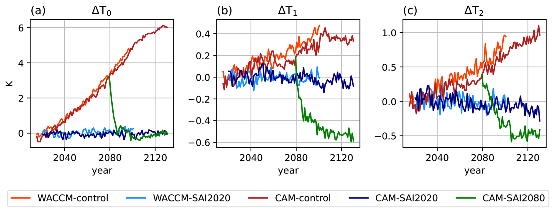
Figure 4 Time series of annually averaged global mean surface temperature, T₀ (a), interhemispheric gradient of surface temperature (i.e. north minus south), T₁ (b) and equator-to-pole gradient of surface temperature (i.e. poles minus equator), T₂ (c), anomalies. Reference values, in K, corresponding to the [2016–2035] period of the control simulations for CAM and [2015–2024] for WACCM, are given by (T_0,ref, T_1,ref, T_2,ref): (288.72, 0.93, −11.70) for CAM and (288.42, 0.84, −11.89) for WACCM.

Table 4 Summary of temperature metrics.

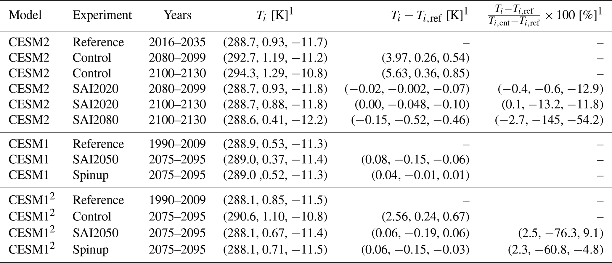
¹ For $i\mathit{ϵ}\mathit{\{}\mathrm{0},\mathrm{1},\mathrm{2}\mathit{\}}{T}_{\mathrm{0}}$: GMST, T₁ interhemispheric gradient (north minus south), T₂: equator-to-pole gradient (pole minus equator); ² high-res: nominal resolution 0.5° atmosphere, 0.1° ocean.

3.1 Surface temperature

3.1.1 Temporal evolution of temperature targets

The change of T₀ with respect to present-day, ΔT₀, is very similar in CAM-SAI2020 and WACCM-SAI2020 (Fig. 4a), showing that the forcing works properly for CAM under the same scenario. In CAM-SAI2080, ΔT₀ adjusts rapidly and approaches zero with moderate overcooling, showing that the forcing also works for a different scenario. For CESM1(CAM), the forcing also works well at similar (Fig. C1a) and higher resolution (Fig. C2a). A slight overcooling of about 0.2 °C in CAM5-SAI2000 is likely the result of a too strong (2 times) initial guess for the feedforward. Changes in GMST in SAI minus Reference are less than 3 % of the changes in Control minus Reference for all SAI experiments (Table 4). These results indicate that T₀ is adequately controlled by the proposed method for all model versions, scenarios and resolutions.

As the aerosol field in CAM changes with global mean AOD similarly to WACCM-SAI2020, model and/or scenario differences may lead to different evolutions of ΔT₁ and ΔT₂. We find that these gradients are very similar between CAM-SAI2020 and WACCM-SAI2020 (Fig. 4b and c). However, in CAM-SAI2080, ΔT₁ and ΔT₂ decrease more than their initial increases due to global warming, suggesting that scenario differences with respect to the WACCM data have a significant effect on these metrics. As discussed below, this is related to changes in the Atlantic Meridional Overturning circulation (AMOC). For CESM1, there are minor decreases of ΔT₁ and ΔT₂ in CAM5-SAI2000 (Fig. C1b and c). The ΔT₁ decrease is likely caused by the overcooling as land cools quicker than ocean. The changes of ΔT₁ and ΔT₂ in CAM5-SAI2050 are far less drastic compared to CAM-SAI2080 (CESM2), confirming the importance of scenario differences. In high-resolution CESM1, ΔT₂ shows little change while ΔT₁ decreases, though also less drastic than CAM-SAI2080 (Table 4). There is a minor decrease of ΔT₁ during the initial adjustment to target temperature, likely due to quick cooling of land surface by high aerosol forcing these years (Fig. C2b and c). In general, ΔT₁ changes by less than 1 % of the change in Control minus Reference for CAM-SAI2020, but 13.2 % in the extended analysis period after 2100 and far more in CAM5-SAI2050 and, especially, CAM-SAI2080 (Table 4). ΔT₂ changes by about 10 % in most experiments, but by 54 % in CAM-SAI2080. As discussed in Sect. 6, residual errors in ΔT₁ and ΔT₂ can likely be addressed by dynamically scaling the interhemispheric and equator-to-pole gradients of the aerosol field during simulation.

3.1.2 Spatial patterns in late-century SAI2020

The annual mean surface temperature change in late-century SAI2020 with respect to present-day is generally very similar between CAM and WACCM, with typical inter-model differences in warming being much less than 1 °C and with similar warming patterns (Fig. 5a–c). This suggests that mechanisms determining the surface temperature change are present in both models, though CAM tends to have stronger warming patterns. The highest similarity in surface temperature change is found in the tropics and subtropics, where there is warming and cooling, respectively. Warmer tropical waters near Peru suggest that the El Niño–Southern Oscillation shifts to a more positive phase. Both atmospheric models show cooling in the North Atlantic, as described in more detail by Pflüger et al. (2024). The largest inter-model differences are in the Arctic region and Northeast Asia, where CAM shows more surface warming than WACCM. This is likely due to a model discrepancy as CAM also has a warmer Arctic region in the Reference period, as shown in Fig. A1, and, to a lesser degree, in the Control simulation. The deviations in the Arctic may also partly stem from the fact that our algorithm only scales the overall strength of the aerosol field, whereas the CESM(WACCM) simulations steer injection rates at four different latitudes. Despite the Arctic warm bias in CAM, the large-scale gradients of surface temperature do not change significantly different in CAM with respect to WACCM (Fig. 4), which is due to the stronger North Atlantic cooling.

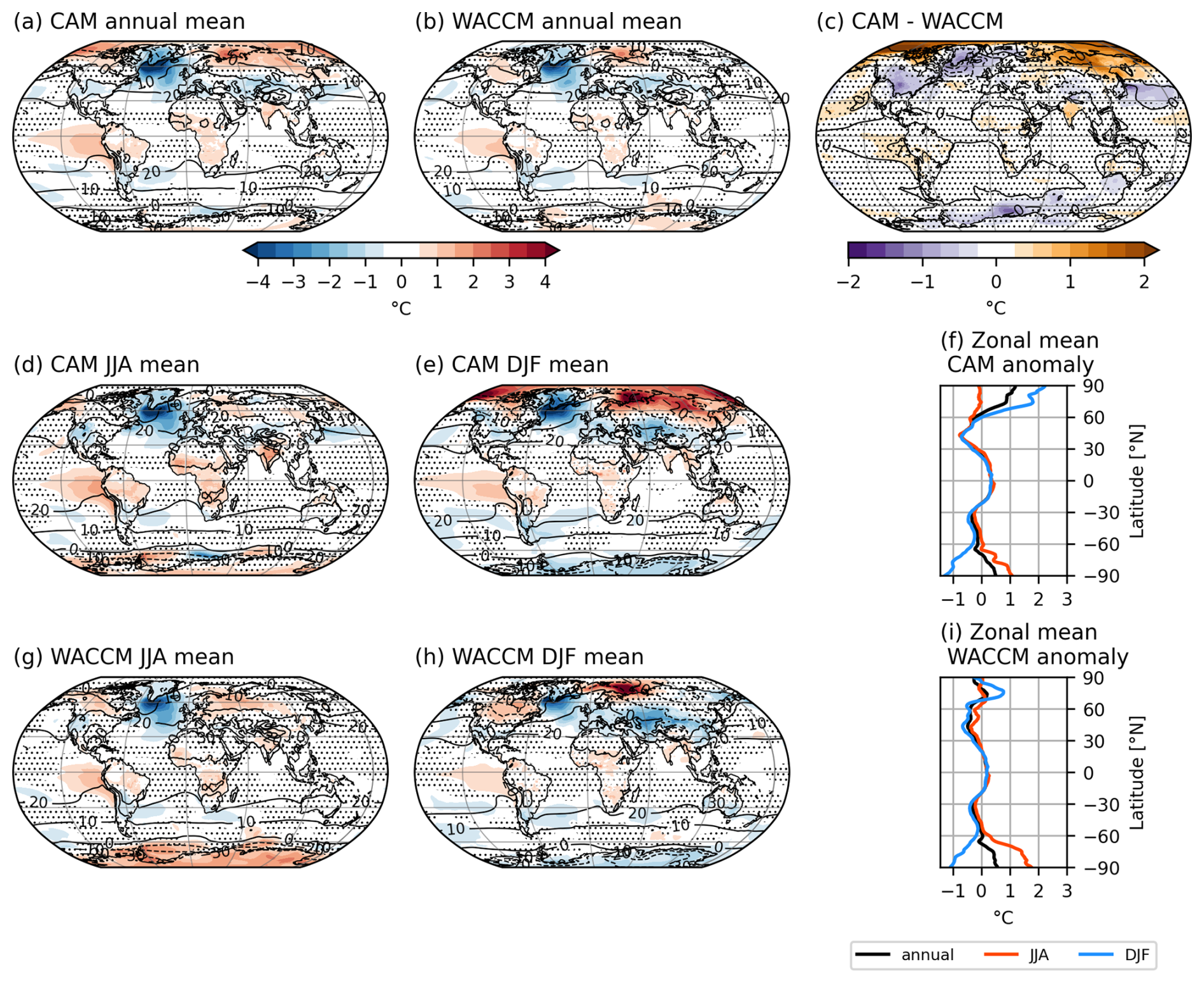
Figure 5 2 m temperature anomalies averaged over [2080–2099] in SAI2020 with respect to present-day. (a, b) Maps of annual mean anomalies in (a) CAM and (b) WACCM. Present-day mean 2 m temperature is shown in black contours in 10 °C intervals; (c) Difference of (a) and (b), WACCM anomaly shown in black contours in 1 °C intervals; (d) as (a) but for JJA, (e) as (a) but for DJF, (f) CAM zonal mean of annual mean (black), JJA mean (red) and DJF mean (blue), (g) as (b) but for JJA, (h) as (b) but for DJF, (i) as (f) but for WACCM. Stippling indicates changes within the 95 % confidence interval, based on interannual variation of the relevant reference dataset (WACCM-SAI2020 minus Reference for panel c).

The Arctic warming anomaly in CAM is attributed to increasing boreal winter temperatures (Fig. 5d–f). Differences in chemistry model and vertical resolution in the stratosphere between CAM and WACCM may influence Arctic winter temperatures, supporting the possibility that the warm bias is caused by model discrepancies. In the Antarctic region, both models show cooling in austral summer and warming in austral winter, i.e. reduced seasonal variability. The typical amplitude of seasonally averaged surface temperature in this region decreases by about 1 °C, except for the strong winter warming in WACCM which reaches about 2 °C.

Without SAI the warming would be far more drastic (Fig. A2b and c). As the surface temperature anomalies are very similar between CAM and WACCM, the proposed method does not significantly alter local physical mechanisms for SAI2020. In CAM-SAI2080, the cooling of the North Atlantic region is stronger (Fig. A3) and causes excess warming in the Southern Hemisphere as GMST is kept constant. However, the surface temperature anomalies are still small compared to those in the Control simulation. Similarly, surface temperature anomalies for CAM5-SAI2050 (Figs. C3 and C4) are small compared to the warming in the Control simulation (not shown), indicating that the proposed method works well for this scenario. As mentioned earlier, the temperature response to greenhouse gas forcing and SAI may be improved by dynamically scaling the large-scale gradients of the aerosol field.

3.2 Precipitation

Precipitation changes in late-century CAM-SAI2020 and WACCM-SAI2020 with respect to present-day show a general drying except near the equator and in the polar regions, where there is wettening (Fig. 6f and i). The drying is most pronounced in the tropics and around 60° N, and to a lesser extent around 50° S, as can be seen from the zonal mean precipitation changes. The equatorial wettening and subtropical drying indicates a strengthening of the Hadley circulation. CAM and WACCM agree relatively well on the zonal mean precipitation change and its seasonal variation, though CAM tends to have somewhat stronger changes. Thus, it appears that the Hadley circulation in CAM is strengthening more than in WACCM. There is less wettening in the Antarctic and larger seasonal variation in the Arctic in CAM than in WACCM. In CESM1, we find that increasing the model resolution does not have a significant impact on the zonal mean precipitation change, even though polar surface temperature changes differ substantially (Fig. C4).

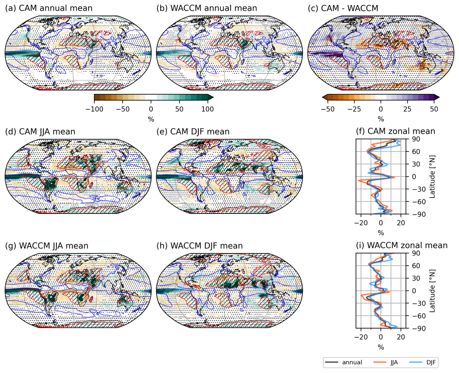
Figure 6 As Fig. 5 but for percentual precipitation changes and with the following remarks: red contours (enclosing hatched regions) indicate 0.5 mm d⁻¹, blue contours 4 mm d⁻¹ precipitation, in (f) and (i), zonal averaging is done before calculating percentual change.

A strengthening and southward expansion of the East-Pacific Inter-Tropical Convergence Zone (ITCZ) in late-century SAI2020 with respect to present-day is found in both models (Fig. 6a and b), but most pronounced in CAM. The East-Pacific equatorial wettening seems to be in part due to a more positive ENSO phase, with DJF drying in the West Pacific and Indonesia, wettening in central North-America (only CAM) and Uruguay (Fig. 6e and h). The stronger East-Pacific equatorial wettening in CAM than in WACCM is likely some inter-model difference as it also occurs in late-century Control (Fig. A1). Changes in the ITCZ in other basins are quite weak, though in high resolution CESM1 we see a southward shift of the Atlantic ITCZ, which is not a clear shift at standard resolution (Fig. C3).

The general drying in late-century SAI2020 with respect to present-day occurs mostly in the subtropics, equatorial West-Pacific and large parts of Eurasia (Fig. 6a–c). CAM shows stronger drying in the Sahel region, Arabia, India and Western Australia than WACCM. This does not seem to be a model bias as the same difference pattern is not visible in late-century Control and present-day (Fig. A1). We suggest that strengthening of the Hadley circulation in late-century SAI2020 with respect to present-day, which is stronger in CAM than WACCM, is related to these local differences. However, further specification is beyond the scope of this work.

Midlatitude winter storm tracks experience little change in precipitation with respect to present-day, though regions that experience change tend to be drying (Fig. 6d–e and g–h). The North Atlantic storm track region seems to shift southwestward, while the South-Atlantic storm track shifts northwestward. CAM and WACCM are in good agreement on the changes regarding the midlatitude winter storm tracks.

Monsoon-affected areas experience less seasonal variation of precipitation in SAI2020 with respect to present-day (Fig. 6d–e and g–h). In DJF, there is drying in Brasil, Central-Africa, and Northern-Australia (wet season) while there is wettening in Colombia, Northern Central-Africa and Southeast Asia (dry season). In JJA, there is drying near Colombia (mostly WACCM), Northern Central-Africa and parts of Southeast Asia (CAM only) (wet season), while there is wettening in Brasil and Southern Central-Africa (dry season). There is in general a good agreement on monsoonal precipitation changes between CAM and WACCM, though summer precipitation in Southeast-Asia increases in WACCM, while CAM shows a more mixed change with wettening in most of China and drying in India, north-eastern China and the Korean peninsula.

3.3 Stratospheric heating and circulation

In addition to reflecting incoming solar radiation, stratospheric sulphate aerosols absorb longwave radiation emitted by the earth. This locally causes up to 10ºC lower-stratospheric warming in late-century SAI2020 with respect to present-day despite the general stratospheric cooling caused by greenhouse gasses. Stratospheric warming is strongest in the (sub)tropics (Fig. 7a and d). The warming pattern closely follows the distribution of sulphate mass (Fig. B1). A minor fraction of the aerosol reaches the high latitudes and, modulated by the polar vortex strength, extend into the polar stratosphere (Fig. 7b–c and e–f). The change in temperature (SAI-Reference) is very similar in both models, i.e. the model difference is small compared to the SAI response (SAI-Control) throughout the troposphere (Fig. A4). This supports that the method is producing desired results.

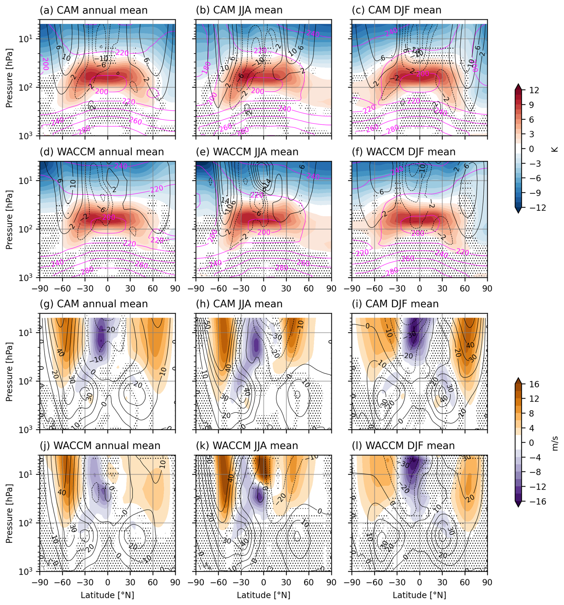
Figure 7 [2080–2090] average SAI2020 anomalies of temperature and zonal wind. Annual (a, d, g, j), JJA (b, e, h, k) and DJF (c, f, i, l) mean anomalies are shown for both models. (a–f) Zonal mean temperature anomaly for CAM (a–c) and WACCM (d–f). Reference zonal mean temperature is shown in magenta contours, zonal mean zonal wind anomalies are shown in black contours; (g–l)`Zonal mean zonal wind anomaly for CAM (g–i) and WACCM (j–l), analogous to (a)–(f). Reference zonal mean zonal wind is shown in black contours. All anomalies are defined with respect to reference period [2016–2035]. Stippling indicates changes within the 95 % confidence interval, based on interannual variation of the relevant reference dataset.

Stratospheric heating due to SAI alters the horizontal pressure gradients and induces an increase of the westerly stratospheric winds at midlatitudes, corresponding mostly to the equatorward side of the polar night jet position. The stratospheric heating in SAI2020 is stronger on the Southern Hemisphere because more aerosol is required to cool down the Southern Hemisphere surface containing more ocean surface. The late-century lower-stratospheric temperature gradient change with respect to present-day causes an increase of the mid-stratospheric annual mean easterly wind between 0–30° S. As shown in Fig. A5, CAM is much colder than WACCM in the polar stratosphere, causing stronger stratospheric westerly jets. The equatorial air mass at 10 hPa is also consistently colder in CAM, increasing the stratospheric easterly equatorial winds. These features occur in Control as well and are assumed to be model differences, most likely related to the upper boundaries of the atmospheric components. The stratospheric wind anomaly in late-century SAI2020 with respect to present-day in both models is similar to the model wind difference (CAM minus WACCM). In the troposphere, changes in wind and temperature are rather small due to the negligible amount of sulphate aerosols and similar surface temperatures.

In CAM(5), ozone is prescribed by the SSP5-8.5 (RCP8.5) scenario. Ozone could have been prescribed by using our proposed method. However, in WACCM, the ozone response due to SAI is much smaller than the ozone increase with time in Control (Fig. B2). More details on ozone in our simulations are provided in Sect. B1 and we discuss the use of prescribed ozone in Sect. 4.

3.4 Performance index

The similarity in SAI response (SAI minus Reference) between CAM and WACCM is assessed using a performance index based on interannual inter-model variability (Fig. 8), defined in Sect. 2.4.

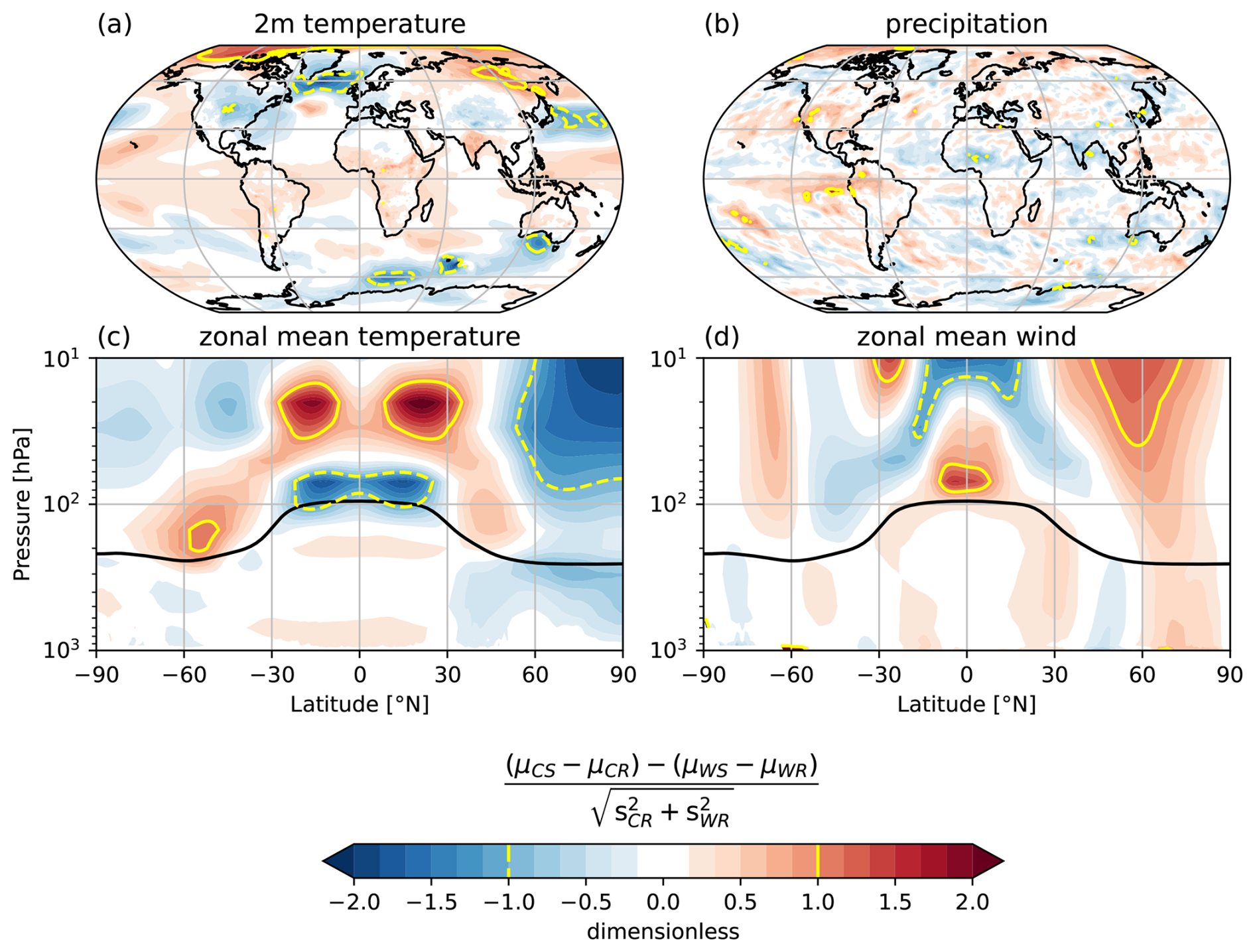
Figure 8 Performance index, as described by Eq. (2), for surface temperature (a), precipitation (b), zonal mean temperature (c) and zonal mean wind (d). Yellow contours indicate index values of (minus) one. The black line shows thermal tropopause pressure in CAM-Reference.

Index values for surface temperature are generally much less than one, indicating that CAM and WACCM tend to have similar responses to SAI in comparison to their interannual inter-model variability. Exceptions include northern high latitude regions, as discussed earlier, and parts of the Southern Ocean and the Western North Pacific. Index values for precipitation are generally much less than one as well. The highest values are seen over small patches across the tropical rainbelts and monsoon regions. For both zonal mean temperature and zonal mean wind, index values are mostly much smaller than one at all latitudes in the troposphere. Inter-model discrepancies are largest in the stratosphere, suggesting that the proposed method may not reliably capture stratospheric effects of SAI. As the method is primarily intended to replicate the tropospheric climate response from WACCM, it is not surprising to see a poor agreement between models in parts of the stratosphere. This can be attributed to the absence of interactive aerosol chemistry and dynamical feedbacks, including ozone breakdown.

4 Discussion

In this study, we applied a pattern-scaling technique to replicate SAI forcing from CESM(WACCM) in CESM(CAM), which lacks interactive stratospheric chemistry, but requires less computational resources. Our aim is to provide a useful tool for modellers, that can be used to generate similar tropospheric climate outcomes in CESM(CAM), can be combined with a feedforward-feedback controller and may be used to model alternate SAI forcing scenarios. The validation results are discussed in Sect. 4.1 and use cases are discussed in Sect. 4.2.

4.1 Validation

Scenarios run with CESM(CAM) achieve GMST targets well in all experiments, multi-year average deviations from target GMST are typically less than 3 % of the GMST change in the control simulation (Table 4). In CAM-SAI2020, the scenario on which the SAI fields are based, these deviations are even less than 0.5 %. Sudden massive cooling scenarios (SAI2080) may show limited (<0.4 K) cooling overshoot. This holds for CESM2, CESM1 and high-res CESM1. By construction, different sensitivities of the models to aerosol forcing do not (to first order) lead to different climate responses, as they are compensated by the feedback controller adjusting the required aerosol forcing (Kravitz et al., 2014). The GMST results suggest that the feedback controller works adequately in combination with the proposed scaling of the forcing field.

For SAI2020, large-scale temperature responses such as the interhemispheric and equator-to-pole gradients (T₁, T₂) are also well reproduced in CAM, with deviations from their respective target values being less than 15 % of their change in the control simulation (Table 4). The regional climate response of surface temperature and precipitation to SAI forcing (with respect to the present-day reference) is largely similar between WACCM and CAM, with differences generally being significantly smaller than interannual inter-model variability (Fig. 8), supporting that the surface climate is adequately controlled in this scenario.

An important difference in SAI2020 is a considerably warmer Arctic in CAM-SAI2020 than in WACCM-SAI2020 (Fig. A1). This is partly due to the fact that CAM has a warmer Arctic in the present-day reference, but partly due to CAM having weaker Arctic winter cooling under SAI (Fig. 5). While CAM6 and WACCM6 share the same physical parameterizations (except for gravity waves) and model grid up to 87 hPa, more detailed chemistry and a higher model top in WACCM6 improves high-latitude climate variability. In particular, WACCM6 exhibits increased East Asian aerosol burdens over CAM6 that extend into the Arctic and affect cloud droplet number and sea ice extent, and therefore temperature (Gettelman et al., 2019). The inter-model difference in surface temperature response to SAI, which tends to amplify the existing model bias in Reference, may therefore be related to differences in model sensitivity to SAI forcing at high latitudes. Another potential reason for the stronger Arctic warming response to SAI in CAM is the slightly stronger aerosol forcing field, which is “tuned” to reduce large-scale temperature gradients in WACCM, not CAM. Deviations in stratospheric temperature and therefore water vapour can have important effects on surface climate (Solomon et al., 2010). The differences between CAM and WACCM in stratospheric sulfate do not exhibit a strong effect in the northern high latitudes only, however (Fig. B1). This suggests that model differences may pay a larger contribution to the warm(ing) bias at northern high latitudes.

Temperature and circulation changes throughout the entire atmosphere in CAM-SAI2020 correspond well to those in WACCM-SAI2020, the deviations being explained by model differences that become quite significant at greater altitudes, i.e. when approaching the model top in CAM (Fig. A5). This is only natural, as CAM lacks interactive stratospheric chemistry, dynamical feedbacks and vertical resolution at these heights. Below the tropopause, the similarity between responses in CAM and WACCM is evident from performance index values much smaller than one (Fig. 8). Therefore, our method is best used to obtain desired climate outcomes below the stratosphere only.

We also studied whether temperature targets can be maintained under a different SAI scenario not modelled in CESM-WACCM. Due to computational constraints, an extensive scan of the scenario space is not attempted, but two delayed onset scenarios that strongly differ from SAI2020, namely CAM-SAI2080 and CAM5-SAI2050 (CESM1), were implemented. In CAM-SAI2080, having 60 additional years of human-induced warming with respect to the scenario from which the aerosol fields are derived, large-scale temperature gradients, not included in the climate target, changed considerably. T₁ decreased by 150 % of the change in the control simulation, and T₂ by 54 % (Table 4). In CAM5-SAI2050, the decrease with respect to Reference of T₁ (T₂) is less than 30 % (15 %) of the decrease in SAI2080, highlighting the important role of onset timing. Changes in the north-south gradient and equator-to-pole gradient of surface temperature are in part explained by North Atlantic cooling. This is because the long period of unmitigated global warming allowed some persistent climate change to build up, in particular AMOC weakening. This weakening is only partially compensated by SAI and decreases poleward heat transport, overcooling the North Atlantic (Pflüger et al., 2024). Its effect on surface temperature is evident as a North Atlantic warming hole (Fig. A3). The impact is dependent on the exact onset of SAI, however, as starting SAI in 2035 or  045 may prevent prolonged weakening of the AMOC (Brody et al., 2024). In a feedback controller with several injection latitudes (as used in WACCM), at least the north-south gradient could probably be reduced after delayed onset by increasing (decreasing) aerosol injection on the Southern (Northern) Hemisphere. In our simple implementation with just one degree of freedom, i.e. a global injection intensity, this is not possible. However, an expansion might be possible (Sect. 6).

Next it is verified whether temperature targets can be maintained in case of a different background climate scenario. The CESM1(CAM5) simulations conducted in this study were initialised from perpetual 2000 conditions, and therefore represent a perturbed climate with respect to the original (transient) CESM1(WACCM) simulations on which the forcing fields are based. Another difference is that a lower CO₂-only RCP8.5 greenhouse gas forcing is used. Changes with respect to Reference in T₁ and T₂ are generally less than 0.25 K (Fig. C1). From this we conclude that temperature targets can be maintained reasonably well against a different background climate scenario. Additionally, changes in temperature metrics in the high-resolution are similar to the changes in the one degree resolution (Fig. C2, Table 4), suggesting that our proposed method is fairly robust against increasing spatial resolution.

In this study, ozone is prescribed by the fixed high-forcing scenarios (SSP5-8.5, RCP8.5). Ozone has an influence on the temperature and dynamics of the stratosphere, mainly through shortwave radiation absorption. Injected sulphate aerosols host heterogeneous reactions that can decrease ozone concentration (Tilmes et al., 2008). Moreover, changes in temperature, moisture and transport due to the aerosols affect chemical ozone losses as well. However, we found relatively minor decreases due to SAI. The limited response of ozone concentration to SAI in WACCM was hypothesized by Kravitz et al. (2019) to result from strongly reduced stratospheric CFC concentrations, preventing the catalytic ozone loss hosted on aerosol surfaces. Recent simulations with WACCM by Tilmes et al. (2021) indicate that high CFC concentrations combined with small aerosol sizes lead to a strong reduction in stratospheric ozone per injected amount in the first decade after onset of SAI. However, this efficiency declines rapidly in subsequent decades, limiting overall ozone loss due to SAI, particularly toward the end of the century – the focus period of our analysis. As ozone seems to depend more strongly on the CFC conditions than AOD, we chose to force CAM with unmodified WACCM SSP5-8.5 ozone concentrations. The specific implementation influences ozone concentrations and, consequently, both stratospheric (Tilmes et al., 2021) and tropospheric climate (Bednarz et al., 2022). While the radiative heating effect of ozone is likely much smaller than that of aerosols, this potential disparity warrants further investigation. In general, prescribing ozone using our proposed method is considered safer and more consistent for capturing ozone changes under SAI scenarios, as it better accounts for chemical and dynamical feedbacks induced by aerosols. Although we did not implement this approach in the present study, the resulting differences were found to be relatively small, and thus the simulations were not repeated.

4.2 Use cases

We believe that our procedure can be useful for several possible applications in which modellers are interested in scenarios achieving some climate target (e.g. GMST) using SAI, in which computation time is a constraint and the focus is on climate impacts below the stratosphere. The relative ease with which the feedback controller method achieves climate target despite different model sensitivities to aerosol forcing is a main benefit of the approach, as it saves the effort of rescaling the forcing per hand. Compared to earlier studies using linear scaling between AOD and other aerosol-related quantities, we approximately capture their non-linear relationship. Nonetheless, we caution that our method should not be used for researching stratospheric impacts of SAI.

The easiest use case is probably mimicking CESM(WACCM) simulations, for example for increasing model resolution in the cheaper CAM model or for generating larger ensembles, because for these applications one does not need to translate between different scenarios.

A more advanced use case is expanding the scenario range in CAM. We have shown that this is in principle feasible (SAI2080), but, depending on the scenario, this requires some care. For SAI2080, we had to adjust the feedforward and manipulate the integrator term in the feedback controller. In addition, as discussed above, a feedback controller with a single degree of freedom may not be able to control all climate targets that were controlled in the underlying multiple-control WACCM simulation. Whether this is worthwhile may depend on the application in question and the accuracy with which one wants to mimic the multi-latitude multi-objective injection scheme (in our case, four injection latitudes and three targets) of the WACCM simulations.

5 Conclusions

Combining prior work on forcing models lacking stratospheric aerosol modules with aerosol fields, and feedback controllers, we developed a procedure to produce SAI simulations in CESM(CAM) – a model version without interactive stratospheric aerosol – by providing automatically scaled input to the volcanic aerosol forcing field. This approach can strongly reduce computation time with respect to CESM(WACCM).

The procedure is validated by imitating a multi-objective CESM(WACCM) SAI forcing scenario in CESM(CAM). Despite having only a single-objective (GMST) control in its current form, all target metrics from the CESM(WACCM) simulation returned to their respective reference values. We looked at four key climate variables and found that their response to SAI is similar in both models, though the models may have slighly different responses locally. The largest differences in reponse to SAI are found in the stratosphere, where absence of interactive chemistry and dynamical feedbacks lead to reduced performance. The differences in response to SAI have been quantified by an index and are found to be generally less or much less than interannual inter-model variability in the troposphere, providing confidence in the ability of the proposed method to produce the desired tropospheric climate.

When delaying the start of SAI in CAM by 60 years, slow climate change effects affect the temperature objectives of the original WACCM simulation. The data shown may serve as a first indication of the magnitude of climate deviations when applying the procedure to a significantly different (SAI2080 vs. SAI2020) forcing scenario.

Similarly, experiments with CESM1(CAM) have shown the robustness of the procedure when applying it to simulations with a different initial climate state, model version and spatial resolution.

6 Outlook

It is likely possible to mimic a multi-objective injection scheme in CESM(CAM) by deriving separate forcing fields from single-latitude injection simulations in CESM(WACCM). If aerosol concentrations from different forcing locations add up approximately linearly, total aerosol fields could be obtained easily. Otherwise, a more complex nonlinear fit between single-latitude injection intensities and aerosol concentrations would be needed, requiring additional input from CESM(WACCM). Recent work on an emulator (Farley et al., 2024) suggests that even climate outcomes (rather than the intermediate step, i.e. the aerosol forcing) can be obtained to reasonable approximation by linear pattern scaling of single-latitude injection outcomes. These techniques may be applied to generate a forcing field with pattern control and combined with our method to generate the full stratospheric forcing fields for CESM(CAM).

A potential future use case is to use SAI forcing derived from CESM(WACCM) (or other models with stratospheric chemistry) also in other models than CESM(CAM). This would allow models without extensive stratospheric chemistry modules to run SAI simulations. In addition, it could help model comparisons by disentangling differences in aerosol processes from differences in climate effects of aerosols.

However, while WACCM and CAM are co-developed consistently with regards to the possibility of using WACCM-output to force CAM, the transfer to other models may be more challenging. For example, some combinations of models require Mie calculation-based conversion tools for the preparation of stratospheric aerosols input data due to a mismatch in prescribed variable definitions. An example of such tool is the REMAPv1 algorithm (Jörimann et al., 2025). While not yet validated for mismatched model output-input formats, future usage may include calculation of the stratospheric forcing fields using our method and consequent transformation using such tools to provide usable input for the lower-complexity model.

If these technical challenges can be resolved, our procedure based on the feedback controller can again help to automatize the scaling of aerosol forcings in line with desired climate targets.

Appendix A: Additional simulation results

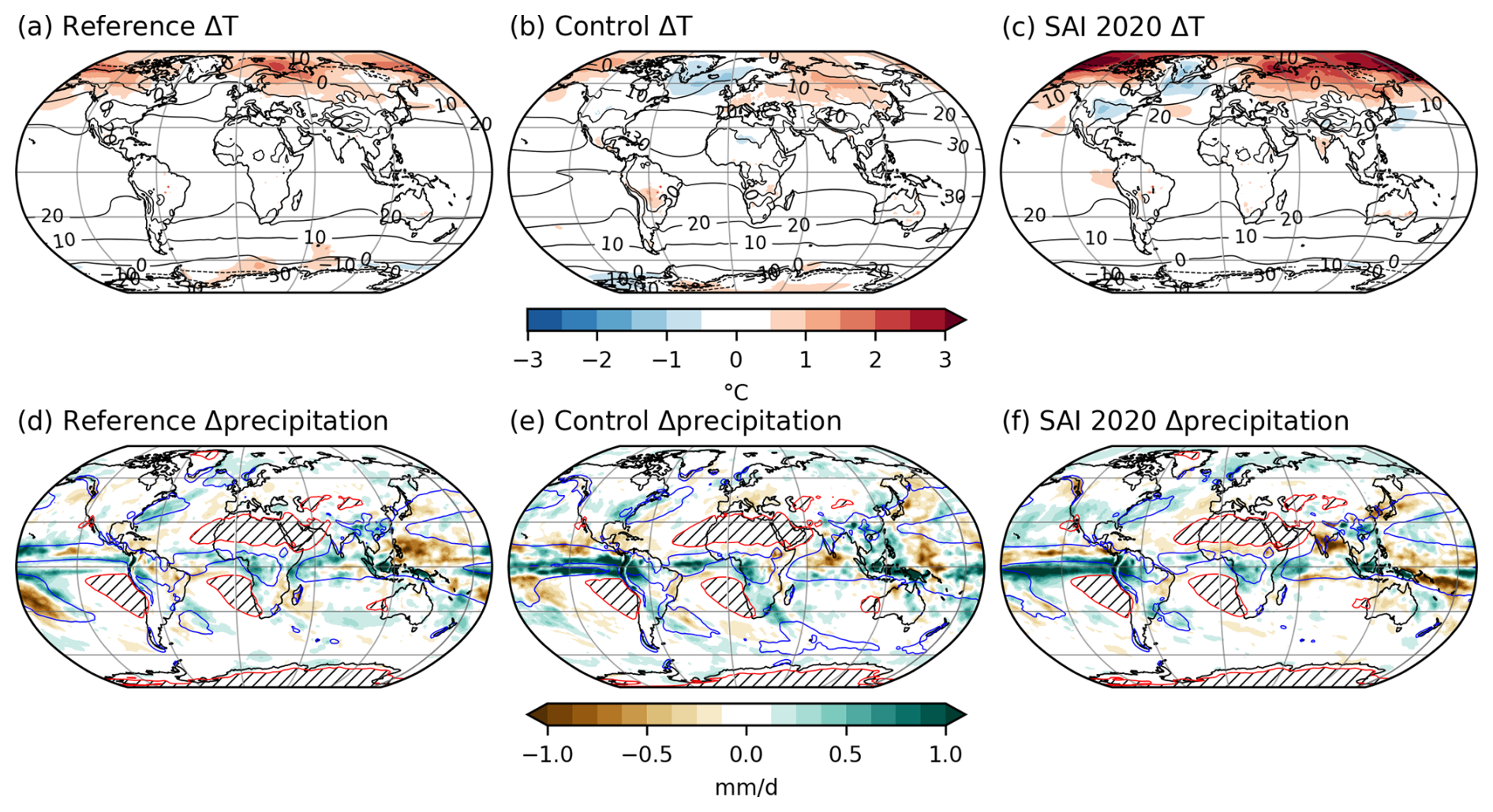
Figure A1 CAM-WACCM model differences of temperature (a–c) and precipitation (d–f). All data are averaged over [2016–2035] (reference) or [2080–2099] (control and SAI2020). Black contours in the temperature maps indicate the corresponding values in WACCM for each experiment. Contoured/hatched regions in the precipitation maps are similar to Fig. A2d–f, but for the respective experiments in WACCM.

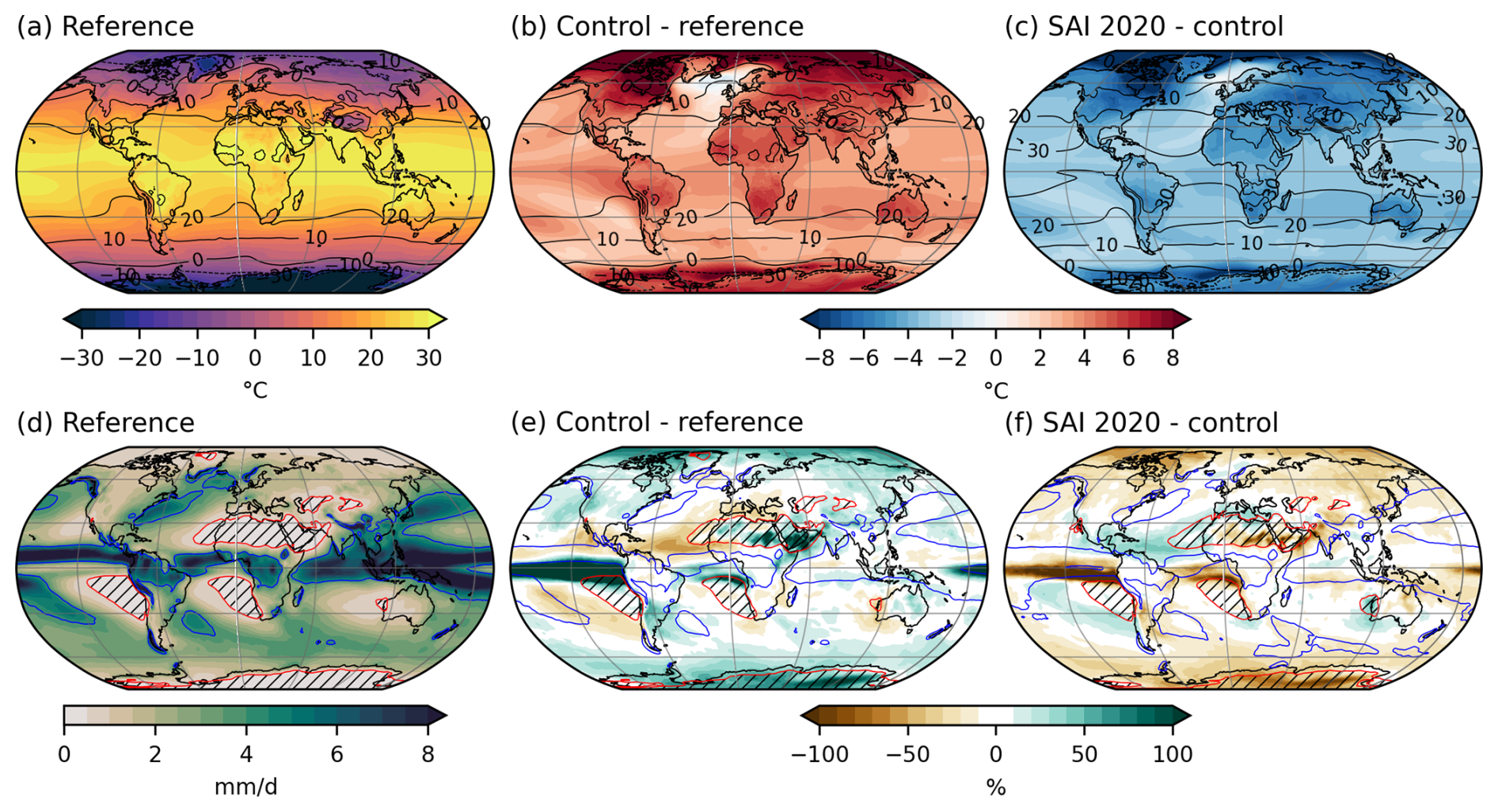
Figure A2 CAM temperature (a–c) and precipitation (d–f) maps showing the present-day (reference) state (a, d), control-reference (b, e) and SAI2020-control (c, f) differences. Control and SAI2020 data are averaged over [2080–2099], reference over [2016–2035]. Black contours in the temperature maps indicate the corresponding values for CAM reference (a, b) and control (c). Hatched regions enclosed by red contours in the precipitation panels have less than 0.5 mm d⁻¹ of precipitation in the CAM reference (d, e) and control (f), whereas blue contours denote 4 mm d⁻¹.

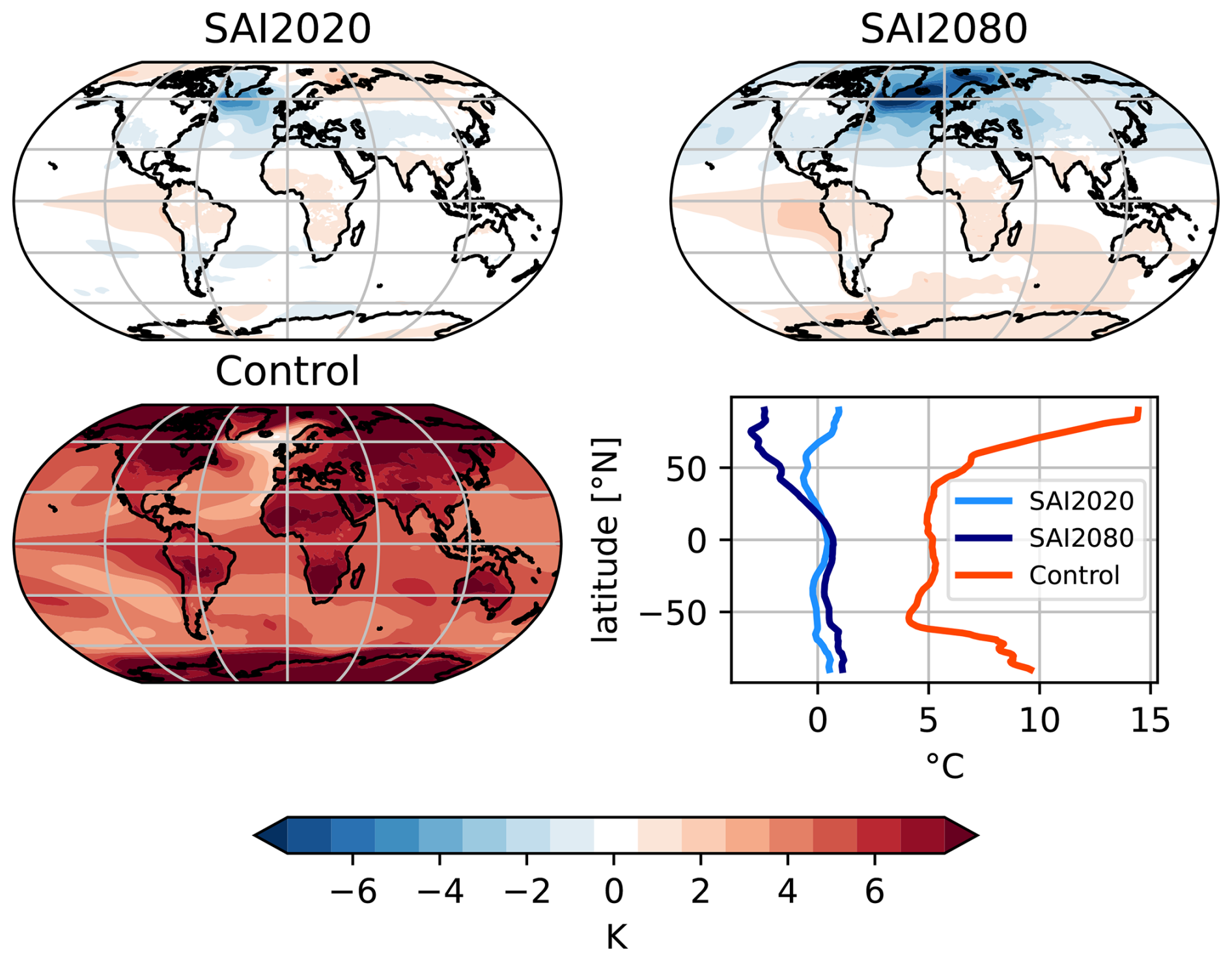
Figure A3 CAM [2100–2129] surface temperature anomalies and their zonal means. The reference period is [2016–2035].

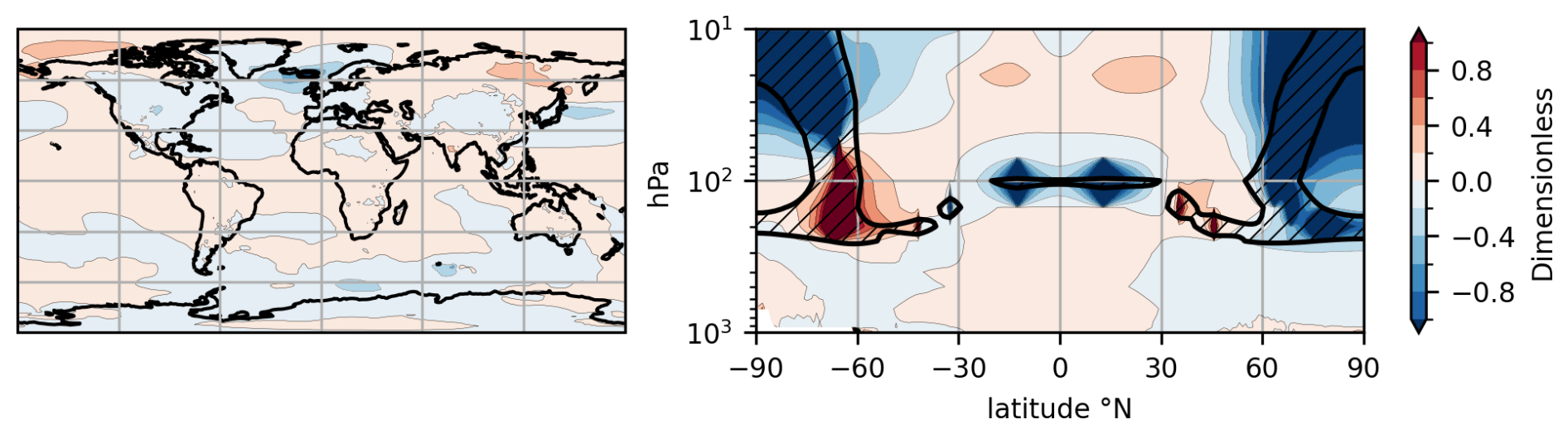
Figure A4 Performance index for surface temperature (left panel) and potential temperature (right panel). The index is the ratio of the model difference of SAI-REF (CAM SAI-REF minus WACCM SAI-REF) and the model-mean SAI response (CAM SAI-CNT + WACCM SAI-CNT)/2. Low values (much smaller than 1) indicate desired results. All data are averaged over [2016–2035] (reference) or [2080–2099] (control and SAI2020). Hatching indicates where the inter-model mean SAI response is smaller than 1 K (left panel) and 2.5 K (right panel), i.e. where the index is less reliable. These values are somewhat arbitrary, choosing larger (smaller) values will make the hatched area larger (smaller).

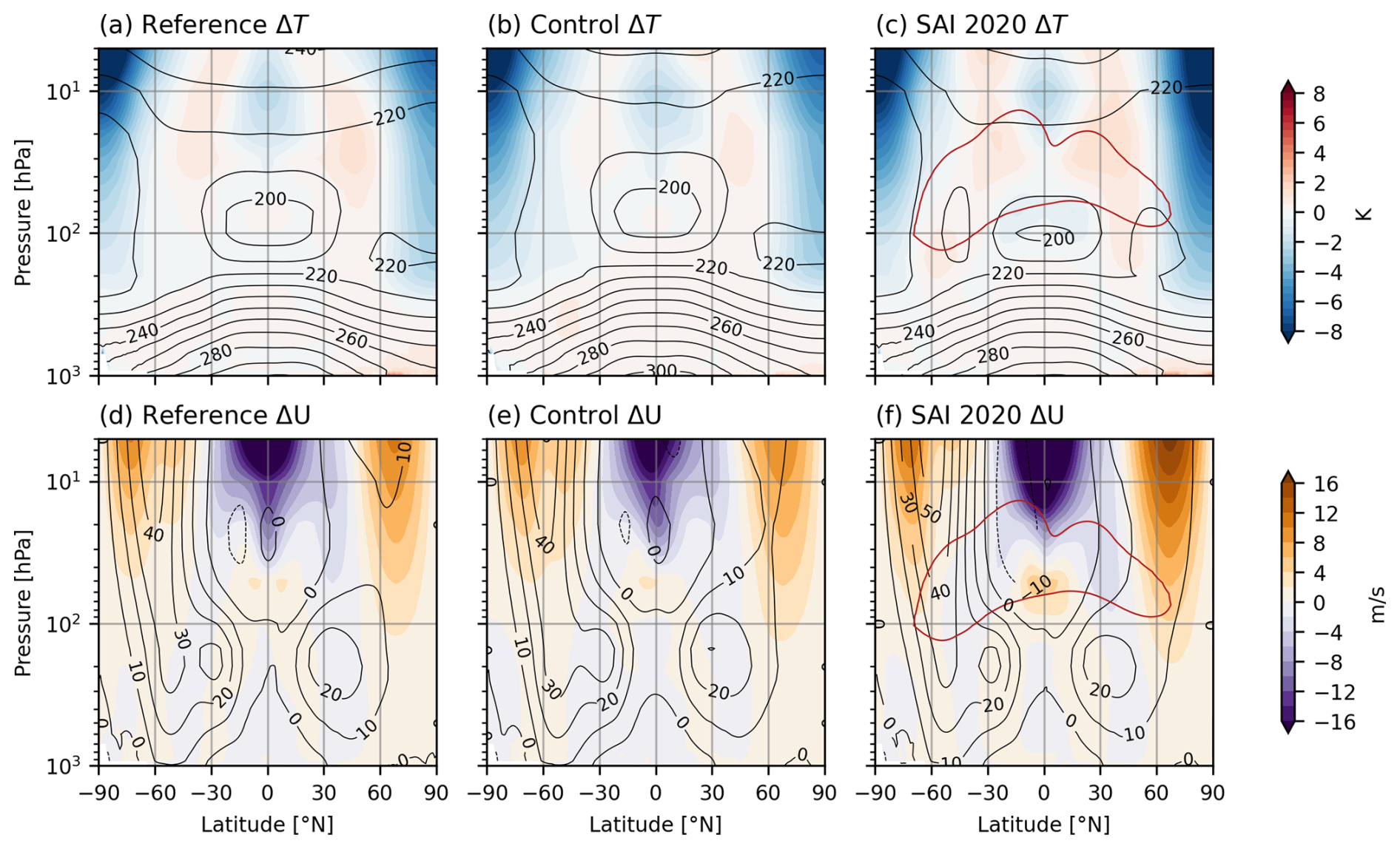
Figure A5 CAM-WACCM model differences of zonal mean temperature (a–c) and zonal mean zonal wind (d–f). All data are averaged over [2016–2035] (reference) or [2080–2099] (control and SAI2020). Black contours in the temperature maps indicate the corresponding values in WACCM for each experiment.

Appendix B: Aerosol distribution

Examinining the relevance of dynamically scaling ozone

Ozone concentrations in WACCM increase significantly with time, most likely due to a reduction in ozone-depleting substances (Fig. B2a). Maximum zonal mean ozone concentration is higher in WACCM-SAI2020 than WACCM-Control, though the difference is small relative to the increase from 2020 to 2100 in both experiments. In CAM, ozone is prescribed following the SSP5-8.5 scenario, which is practically identical to ozone in WACCM-Control.

A more detailed view of the zonal mean ozone difference between WACCM-SAI2020 and WACCM-Control is shown in Fig. B2b. In the lower stratosphere, ozone change follows a slightly complicated pattern. As a response to SAI In WACCM simulations with interactive ozone chemistry, Richter et al. (2017) find stratospheric ozone concentration increases above the sulphate aerosol layer, while it decreases inside, with a reversed pattern on the opposite hemisphere for hemispheric injection. This pattern may be recognized in the current reference WACCM simulation given more aerosols are injected on the Southern Hemisphere than the Northern Hemisphere (Fig. B1b), though this is just an observation and further explanation is beyond the scope of this study. In the upper stratosphere, ozone concentrations generally decrease due to SAI in WACCM, most notably at the poles. These effects naturally lack in CAM, because ozone is prescribed by the SSP5-8.5 scenario. As a consequence, upper-stratospheric polar ozone concentrations in CAM-SAI2020 are higher than in WACCM-SAI2020 (Fig. B2c and f).

The increase of stratospheric ozone concentration with time is much larger than its response to SAI (Fig. B2b, d, and ). Note that, because prescribed stratospheric ozone in CAM is virtually identical to stratospheric ozone in WACCM-Control, (b) may be interpreted as the difference (e) minus (d) and (d) as the change in ozone from the reference to the control period in CAM- and WACCM-Control. This increase contributes to warming above the aerosol layer by increased radiation absorption, however the effect of radiative cooling due to increases greenhouse gas concentrations is stronger (Fig. 7). Hence, the impact of SAI on ozone is relatively minor compared to the effect of reducing ozone-depleting substances in SSP5-8.5, and the effect on climate is likely small. Furthermore, the effect of model differences on stratospheric temperature and circulation is much stronger than the effect of ozone, resulting in significantly colder polar stratospheric temperatures and stronger stratospheric jets in CAM (Fig. A5).

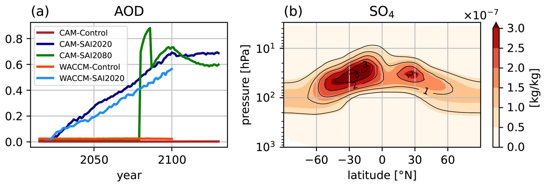
Figure B1 Annual mean global mean aerosol optical depth (a) and prescribed zonal mean sulphate aerosol mass concentration (b) in CAM-SAI2020 (shading) and WACCM-SAI2020 (black contours). Aerosol optical depth represents the stratospheric component of aerosol optical depth at 550 nm (day, night), except for WACCM-control where it is the AOD at 550 nm due to sulphate aerosol (for data availability reasons). The zonal mean sulphate concentration is averaged over [2080–2099] in both CAM and WACCM, and has units 10⁻⁷ kg kg⁻¹.

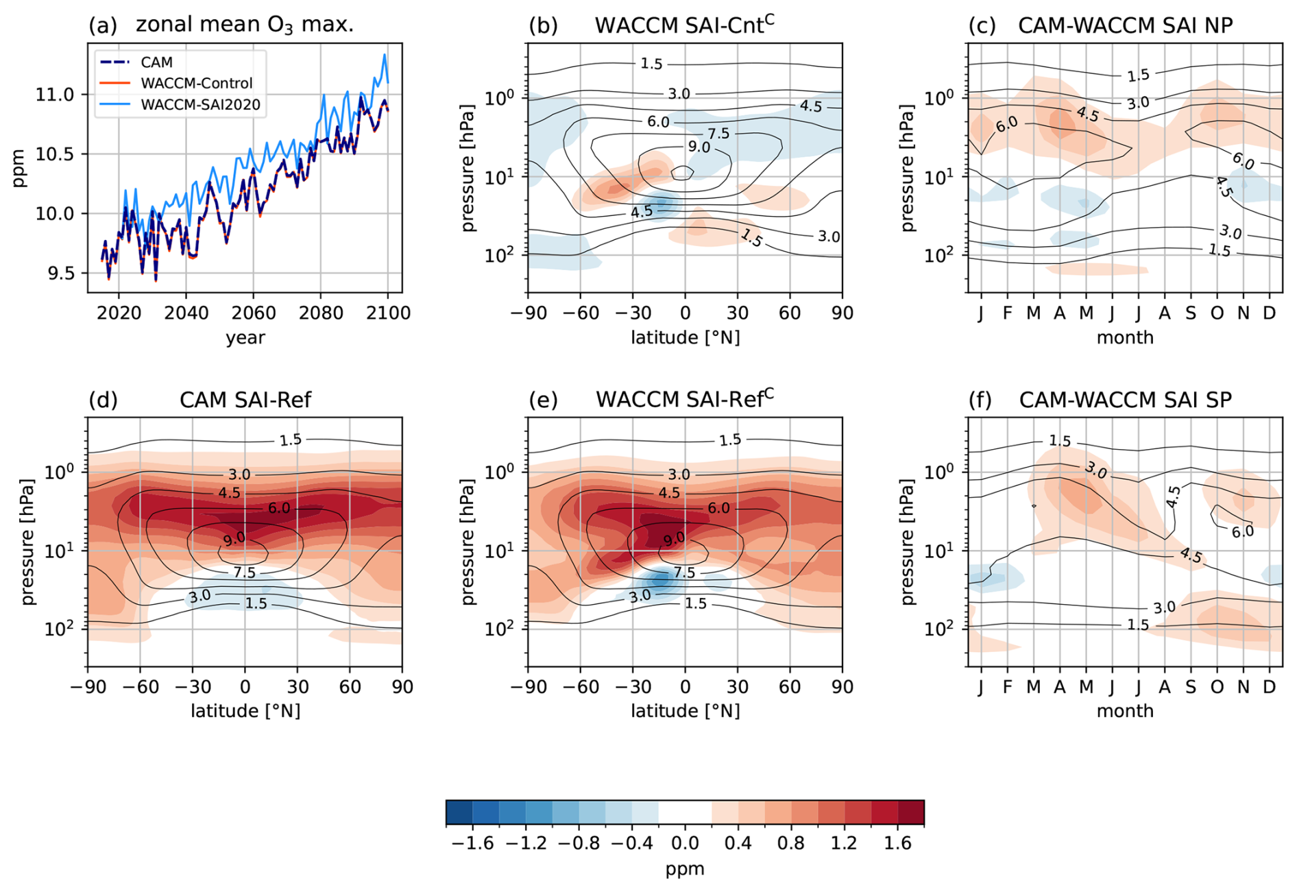
Figure B2 Changes in zonal mean and polar mean ozone. (a) Evolution of maximum zonal mean ozone, (b) zonal mean ozone response to SAI in WACCM, (c) model difference of interannual mean ozone averaged over [60–90° N], (d) temporal change of zonal mean ozone in CAM-SAI2020, (e) temporal change of zonal mean ozone in WACCM-SAI2020, (f) model difference of interannual mean ozone averaged over [60–90° S]. Contours indicate mean ozone for CAM-Control (b), CAM-Reference (d, e) and WACCM-SAI2020 (c, f). WACCM-Control data is available only on 19 pressure levels with relatively poor resolution in the upper stratosphere, whereas all other data is provided on 70 vertical levels. Ozone in CAM is prescribed by the SSP5-8.5 scenario, which is virtually identical to WACCM-Control. Therefore, CAM data is substituted for WACCM-Control data (indicated with a superscript C) in all panels except (a), where the coarse levels are used. In (a), the maximum of the zonal mean is used because the coarse levels do not extend into the upper stratosphere (<3 hPa), making the maximum a more robust representation of the field than a vertically integrated value.

Appendix C: Simulation with CESM1

While the main results are shown only for CESM2(CAM)6 simulations, similar experiments have been performed CESM1.0.4(CAM5). For this configuration, the regressions are performed using data from the Geoengineering Large ENSemble (GLENS) simulations with CESM1(WACCM) (Tilmes et al., 2018). An overview of these simulations is presented in Table 1 and methods and results from the regression analysis are shown in Table C1.

Unlike the CESM2(CAM)6 configuration, the CESM1 configurations require modifications to the applied forcing as the prescribed volcanic aerosol has one size mode, whereas the CESM1(WACCM) output has three modes. To convert from three modes to one, regressions are performed on each of the CESM1(WACCM) modal variables, though only mass mixing ratio is required for CESM1(CAM) (wet diameter is “fixed”). Then, every model year the modal mass mixing ratios are calculated using Eq. (1) in Sect. 2.2 and summed to get the mass mixing ratio of volcanic aerosol.

Table C1 Interannual normalization definitions CESM1.

∫ … dS = annual mean global surface mean, ∫ … dV = annual mean mass-weighted volume integral over the entire atmosphere.

C1 CESM1 climate results

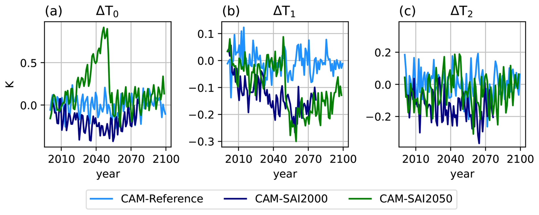
Figure C1 Annual mean anomalies of the global mean temperature, T₀ (a), the interhemispheric gradient of surface temperature, T₁ (b), and the equator-to-pole gradient of surface temperature, T₂ (c) for CESM1.0.4. The anomalies are defined with respect to the [1990–2009] mean CAM5-Reference (perpetual 2000 conditions spinup, light blue) data, giving $T_{\mathrm{0},\mathrm{ref}}=\mathrm{288.92}$ K, $T_{\mathrm{1},\mathrm{ref}}=\mathrm{0.53}$ and $T_{\mathrm{2},\mathrm{ref}}=-\mathrm{11.32}$.

Figure C2 Similar to Fig. C1, but for high-res CESM1. The reference values are $T_{\mathrm{0},\mathrm{ref}}=\mathrm{288.08}$ K, $T_{\mathrm{1},\mathrm{ref}}=\mathrm{0.85}$ and $T_{\mathrm{2},\mathrm{ref}}=-\mathrm{11.47}$.

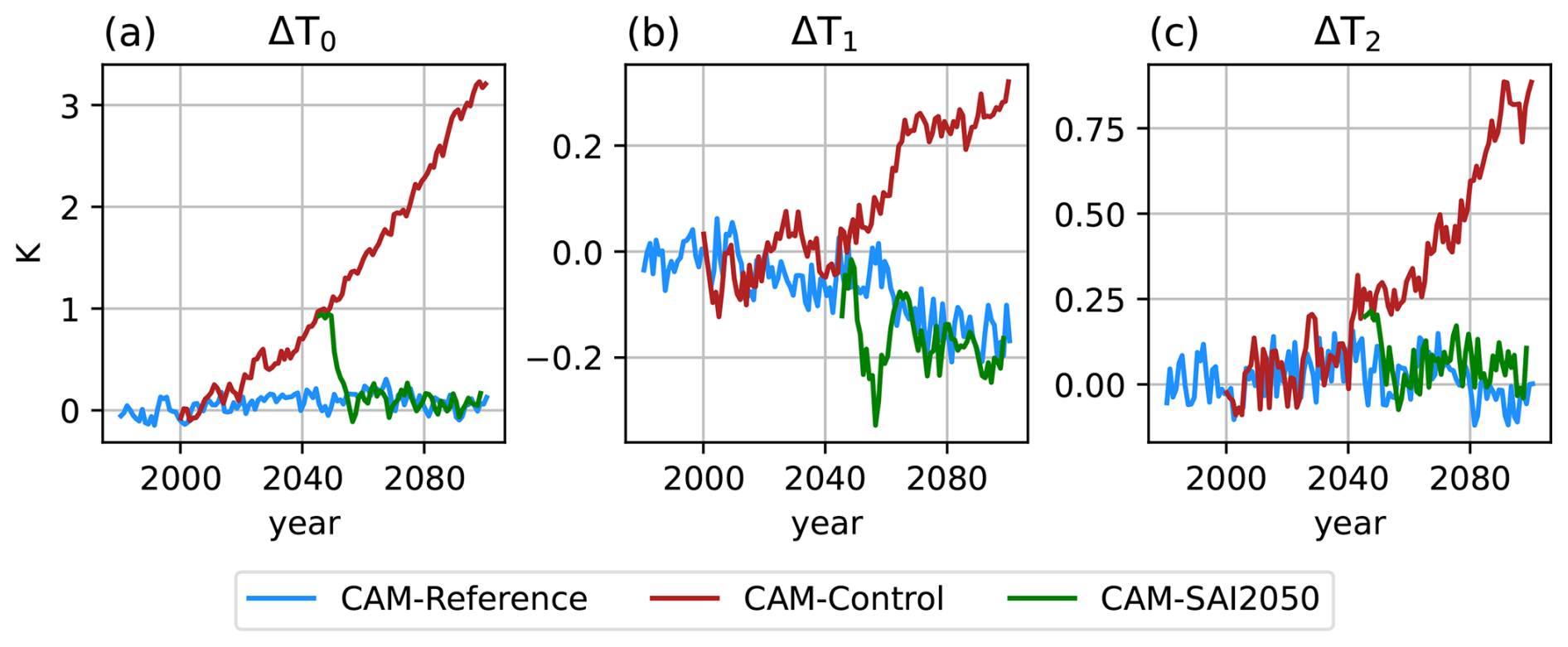
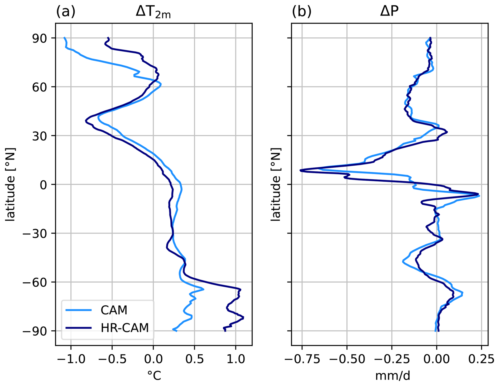
Figure C3 [2075–2095] surface temperature anomalies (a, b) and precipitation anomalies (c, d) for CESM1. The anomalies are shown for CAM (a, c) and HR-CAM (b, d), having a nominal resolution of 1 and 0.5°, respectively. Contours represent the reference values, which are drawn at 0.5 mm d⁻¹ (red, hatched) and 4 mm d⁻¹ (blue) for precipitation. The reference period is [1990–2009].

Figure C4 Similar to Fig. C3, but showing the zonal means.