JuWavelet – continuous wavelet transform and S transform for wave analysis

This paper describes the Python package JuWavelet, which implements the continuous wavelet transform using the Morlet wavelet, which is a popular tool in the geosciences to analyse wave-like phenomena. It closes a gap in available software, which is typically focused on discrete transforms or lower dimensions than offered here. The code implements the transform in 1-D, 2-D, and 3-D. In particular, not only the analysis but also the synthesis from a (modified) decomposition is available. It also provides a consistent implementation for both the original continuous wavelet transform and the derivative and arguably superior S transform popular in atmospheric gravity wave analysis for all dimensions.

This paper documents the mathematics behind the implementation and offers several examples to showcase the capabilities of the software including the code to generate the figures shown.

1 Introduction

Since the introduction of the continuous wavelet transform (CWT) by Grossmann and Morlet (1984), it has been used extensively in the geophysical sciences. In particular the Morlet wavelet, being a harmonic oscillation with a Gaussian envelope, is uniquely useful for the analysis of wave-like phenomena (e.g. Meyers et al., 1993). The papers by Stockwell et al. (1996) and Torrence and Compo (1998) further popularized the transform in the geophysical sciences. Since then, the CWT and the special “flavour” of CWT introduced by Stockwell labeled S-transform (ST) have been mainstays in the analysis of atmospheric gravity waves (e.g. Kaifler et al., 2015; Chen and Chu, 2017; Ghil et al., 2002; Hindley et al., 2019; Kaifler et al., 2023; Reichert et al., 2024). While not named as such by its inventor, the S transform is sometimes also labelled Stockwell transform.

As exemplary structures for our examples, we use atmospheric gravity waves (GWs), which are internal GWs in a stably stratified medium reflecting the interplay between gravity and buoyancy force (Nappo, 2012). Due to their 3-D propagation 2-D horizontal cross sections of temperature fields, obtained for instance by the Atmospheric InfraRed Sounder (AIRS) or by numerical models, show spatially localized wave packets with only few oscillations (e.g. Hindley et al., 2019; Jiang et al., 2019). But GW packets are also localized in the frequency domain since spectral properties are functions of atmospheric background conditions that can change quickly (Reichert et al., 2024). This localized nature of GWs requires a time–frequency or space–wavenumber analysis tool such as the CWT or ST. While we use only atmospheric gravity waves and synthetic data for our examples, the method is well suited for analysing any signal with localized wave-like structures. This paper focuses on the general and pure CWT approach, but dedicated tools for GW analysis have been created using similar techniques. Of recent note are the few-wave decomposition (S3D) by Lehmann et al. (2012), which is focused on high-performance 3-D analysis based on short-time Fourier transform (STFT)-like techniques, and the Unified Wave Diagnostics by Schoon and Zuelicke (2018) based on the Hilbert transform.

Wavelets can be defined in any number of dimensions, but most geophysical applications deal with only 1-D, 2-D, or 3-D data. While the literature describing the transform and analysing data of these dimensionalities is available (e.g. the 2-D analysis by Chen and Chu (2017) or a 3-D analysis by Hindley et al., 2019), properly validated code is only freely available associated with the publication of Torrence and Compo (1998), providing the 1-D CWT only. This paper tries to close this gap by describing the open-source JuWavelet package, which provides 1-D, 2-D, and 3-D implementations in the widely used Python programming language of the CWT using the Morlet wavelet, as well as the associated ST. Following the equations provided by this paper allows us to fully validate both the algorithm and the implementation and should also allow the development of derivative work such as a 4-D analysis, the use of different wavelet basis functions, or the translation of the code in a different programming language. Earlier versions of this software were already used for the publications of Geldenhuys et al. (2023) and Krasauskas et al. (2023). The intent is to make this analysis method more readily available and to provide a starting point for modifications of the algorithm to suit the scientific need at hand.

We first introduce the mathematics behind the CWT and its discretization in 1-D. We keep the higher-dimensional formulas in the Appendix for brevity's sake. A comprehensive and rigorous treatise on wavelets in general can be found in textbooks as provided by, for example, Mallat (1999), the notation of whom we follow here. Second, we describe the CWT using the Morlet wavelet and the S transform in greater detail including several application notes helpful for users of the software package. Third, we exemplarily explain the call of the 2-D decomposition in detail. Lastly, we give some examples of the use of the software package. A particular highlight of the overdetermined CWT (and ST) is the ability to not only analyse the data for signals of certain frequencies but also extract features from this. This requires the proper implementation of the inversion of the transform documented below, which this software delivers as well.

2 Continuous wavelet transform

This section gives a very brief and mathematical introduction of the CWT and its inversion, here called reconstruction. Emphasis is put on the discretization necessary to apply the continuous transform on sampled data on a computer. Here, we always assume that there is a continuous function behind the samples, which is our actual target of interest. The basic idea behind the CWT is to transform a function from its original space into a function operating on a higher dimensional space, which spans both the original spatial (or temporal) dimension(s) and, in addition, dimensions of wavelength/period. This higher-dimensional function then allows for the easier analysis and modification of the original signal. First we present the mathematics behind the transform, its inverse, and the necessary discretization employed for the implementation at hand. While the software necessarily treats discrete data, we stress that both inputs and outputs of the implementation are to be interpreted as samples of continuous functions.

Given an square-integrable function (typically complex-valued) ψ with zero average and L2-norm of 1, a wavelet dictionary can be constructed by translations and scaling of ψ:

$${\left\{{\mathit{\psi }}_{u,s}\left(t\right)={\displaystyle \frac{\mathrm{1}}{\sqrt{s}}}\mathit{\psi }\left({\displaystyle \frac{t-u}{s}}\right)\right\}}_{u\in \mathbb{R},s\in {\mathbb{R}}^{+}}.$$

These basis functions are normalized with $\left|\left|{\mathit{\psi }}_{u,s}\right|\right|=\mathrm{1}$ (using here and later the L2 norm). The CWT operator W applied to the function f∈L²(ℝ) is then defined as

$$\begin{array}{}\text{(1)}& Wf(u,s)=<f,{\mathit{\psi }}_{u,s}>=\underset{-\mathrm{\infty }}{\overset{\mathrm{\infty }}{\int }}f\left(t\right){\displaystyle \frac{\mathrm{1}}{\sqrt{s}}}{\mathit{\psi }}^{*}\left({\displaystyle \frac{t-u}{s}}\right)\mathrm{d}t.\end{array}$$

The CWT can be defined for complex-valued functions as well, but this has less practical relevance for the application to geophysical data and is thus neglected here. Due to the convolution theorem, this can be computed more efficiently in Fourier space as

$$\begin{array}{}\text{(2)}& Wf(u,s)=\underset{-\mathrm{\infty }}{\overset{\mathrm{\infty }}{\int }}\widehat{f}\left(\mathit{\omega }\right)\sqrt{s}{\left[\widehat{\mathit{\psi }}\left(s\mathit{\omega }\right)\right]}^{*}{e}^{i\mathrm{2}\mathit{\pi }\mathit{\omega }u}\mathrm{d}\mathit{\omega },\end{array}$$

with $\widehat{\cdot }$ denoting the Fourier transform of a function¹. The ^* denotes the complex conjugate. This function also explains the implementation of the transform in the software best, with the exception of being discretized and using the fast Fourier transform instead of the continuous one.

Let $\mathit{\psi }\in L^{\mathrm{2}}(\mathbb{R},\mathbb{C})$ be a complex-valued wavelet with

$$\mathrm{0}<C_{\mathit{\psi }}:=\underset{\mathrm{0}}{\overset{\mathrm{\infty }}{\int }}{\displaystyle \frac{\left|\widehat{\mathit{\psi }}\right(\mathit{\omega }){|}^{\mathrm{2}}}{\mathit{\omega }}}\mathrm{d}\mathit{\omega }<\mathrm{\infty }.$$

Then, W can be inverted (under sensible assumptions on f; Mallat, 1999) as

$$f\left(t\right)={\displaystyle \frac{\mathrm{2}}{C_{\mathit{\psi }}}}\mathrm{Re}\left(\underset{\mathrm{0}}{\overset{\mathrm{\infty }}{\int }}\underset{-\mathrm{\infty }}{\overset{\mathrm{\infty }}{\int }}Wf(u,s){\displaystyle \frac{\mathrm{1}}{\sqrt{s}}}\mathit{\psi }\left({\displaystyle \frac{t-u}{s}}\right)\mathrm{d}u{\displaystyle \frac{\mathrm{d}s}{s^{\mathrm{2}}}}\right).$$

This also conserves the energy of f:

$$\begin{array}{}\text{(3)}& \underset{-\mathrm{\infty }}{\overset{\mathrm{\infty }}{\int }}{\left|f\left(t\right)\right|}^{\mathrm{2}}\mathrm{d}t={\displaystyle \frac{\mathrm{2}}{C_{\mathit{\psi }}}}\underset{\mathrm{0}}{\overset{\mathrm{\infty }}{\int }}\underset{-\mathrm{\infty }}{\overset{\mathrm{\infty }}{\int }}{\left|Wf(u,s)\right|}^{\mathrm{2}}\mathrm{d}u{\displaystyle \frac{\mathrm{d}s}{s^{\mathrm{2}}}}.\end{array}$$

In practice, a different, simpler reconstruction formula is used. Due to the redundancy of the CWT, other functions can also be used instead of ψ for the reconstruction. Holschneider and Tchamitchian (1991) give the necessary conditions for such a function and the proof. One typically uses the Dirac delta function δ as this greatly simplifies the computation of the reconstruction formula:

$$f\left(t\right)={\displaystyle \frac{\mathrm{1}}{C_{\mathit{\delta }}}}\mathrm{Re}\left(\underset{\mathrm{0}}{\overset{\mathrm{\infty }}{\int }}Wf(t,s){\displaystyle \frac{\mathrm{1}}{\sqrt{s}}}{\displaystyle \frac{\mathrm{d}s}{s}}\right)$$

with $C_{\mathit{\delta }}=\mathrm{Re}\left({\int }_{\mathrm{0}}^{\mathrm{\infty }}\frac{\widehat{\mathit{\psi }}\left(\mathit{\omega }\right)\widehat{\mathit{\delta }}\left(\mathit{\omega }\right)}{\mathit{\omega }}\mathrm{d}\mathit{\omega }\right)$. It has the added advantage that only the wavelet transform evaluated at location t is required to reconstruct f at this location, which is perfect keeping in mind that we can only sample the CWT at discrete locations on a computer.

So, to allow numerical fast execution on computers, we apply discretization. First, we discretize the scales s. The data that we analyse are normally sampled and finite and thus band-limited, such that only a finite interval of scales is relevant for the analysis at hand. It is also useful to sample the scales in a logarithmic fashion: $s=s_{\mathrm{0}}{\mathrm{2}}^{d_{j}j}$ following Torrence and Compo (1998), with j∈ℝ for the first step and a natural number in the second step in the following equation. d_j determines the sampling density and is often in the order of $\frac{\mathrm{1}}{\mathrm{8}}$ to $\frac{\mathrm{1}}{\mathrm{2}}$. If we assume that only scales between s₀ and $s_{\mathrm{1}}=s_{\mathrm{0}}{\mathrm{2}}^{d_j(j_s-\mathrm{1})}$, with j_s∈ℕ, are of relevance (e.g. because the original function is band-limited), the reconstruction formula thus becomes by substitution

$$\begin{array}{rl}f\left(t\right)& ={\displaystyle \frac{\mathrm{1}}{C_{\mathit{\delta }}}}\mathrm{Re}\left(\underset{-\mathrm{\infty }}{\overset{\mathrm{\infty }}{\int }}Wf(t,s_{\mathrm{0}}{\mathrm{2}}^{j{d}_j}){\displaystyle \frac{d_j\ln \mathrm{2}}{\sqrt{s_{\mathrm{0}}{\mathrm{2}}^{j{d}_j}}}}\mathrm{d}j\right)\\ & \approx {\displaystyle \frac{\mathrm{1}}{C_{\mathit{\delta }}}}\mathrm{Re}\left(\underset{\mathrm{0}}{\overset{j_s-\mathrm{1}}{\int }}Wf(t,s_{\mathrm{0}}{\mathrm{2}}^{j{d}_j}){\displaystyle \frac{d_j\ln \mathrm{2}}{\sqrt{s_{\mathrm{0}}{\mathrm{2}}^{j{d}_j}}}}\mathrm{d}j\right)\\ & \approx {\displaystyle \frac{\mathrm{1}}{C_{\mathit{\delta }}}}\mathrm{Re}\left(\sum _{j=\mathrm{0}}^{j_s-\mathrm{1}}Wf(t,s_{\mathrm{0}}{\mathrm{2}}^{j{d}_j}){\displaystyle \frac{d_j\ln \mathrm{2}}{\sqrt{s_{\mathrm{0}}{\mathrm{2}}^{j{d}_j}}}}\right).\end{array}$$

This formula can also be used to compute C_δ more easily as the equation also holds for f being the Dirac delta. With

$$\begin{array}{rl}W\mathit{\delta }(u,s)& =\underset{-\mathrm{\infty }}{\overset{\mathrm{\infty }}{\int }}\widehat{\mathit{\delta }}\left(\mathit{\omega }\right)\sqrt{s}{\left[\widehat{\mathit{\psi }}\left(s\mathit{\omega }\right)\right]}^{*}{e}^{i\mathrm{2}\mathit{\pi }\mathit{\omega }u}\mathrm{d}\mathit{\omega }\\ & =\underset{-\mathrm{\infty }}{\overset{\mathrm{\infty }}{\int }}\sqrt{s}{\left[\widehat{\mathit{\psi }}\left(s\mathit{\omega }\right)\right]}^{*}{e}^{i\mathrm{2}\mathit{\pi }\mathit{\omega }u}\mathrm{d}\mathit{\omega }\end{array}$$

follows

$$\begin{array}{rl}\mathit{\delta }\left(\mathrm{0}\right)=\mathrm{1}& \approx {\displaystyle \frac{\mathrm{1}}{C_{\mathit{\delta }}}}\mathrm{Re}\left(\sum _{j=\mathrm{0}}^{j_s-\mathrm{1}}\underset{-\mathrm{\infty }}{\overset{\mathrm{\infty }}{\int }}\sqrt{s_{\mathrm{0}}{\mathrm{2}}^{j{d}_j}}{\left[\widehat{\mathit{\psi }}\left(s_{\mathrm{0}}{\mathrm{2}}^{j{d}_j}\mathit{\omega }\right)\right]}^{*}\right.\\ & \left.\cdot e^{i\mathrm{2}\mathit{\pi }\mathit{\omega }\mathrm{0}}\mathrm{d}\mathit{\omega }{\displaystyle \frac{d_j\ln \mathrm{2}}{\sqrt{s_{\mathrm{0}}{\mathrm{2}}^{j{d}_j}}}}\right)\\ & ={\displaystyle \frac{\mathrm{1}}{C_{\mathit{\delta }}}}\mathrm{Re}\left(\sum _{j=\mathrm{0}}^{j_s-\mathrm{1}}{d}_j\ln \mathrm{2}\underset{-\mathrm{\infty }}{\overset{\mathrm{\infty }}{\int }}{\left[\widehat{\mathit{\psi }}\left(s_{\mathrm{0}}{\mathrm{2}}^{j{d}_j}\mathit{\omega }\right)\right]}^{*}\mathrm{d}\mathit{\omega }\right)\end{array}$$

and thus

$$C_{\mathit{\delta }}\approx d_j\ln \mathrm{2}\sum _{j=\mathrm{0}}^{j_s-\mathrm{1}}\mathrm{Re}\left(\underset{-\mathrm{\infty }}{\overset{\mathrm{\infty }}{\int }}{\left[\widehat{\mathit{\psi }}\left(s_{\mathrm{0}}{\mathrm{2}}^{j{d}_j}\mathit{\omega }\right)\right]}^{*}\mathrm{d}\mathit{\omega }\right).$$

3 The Morlet wavelet and the S transform

In the field of geophysics the use of the Morlet wavelet is historically very popular (e.g. in the fields of seismology, Grossmann and Morlet, 1984, oceanography, Meyers et al., 1993; Torrence and Compo, 1998, and atmospheric gravity waves, Chen et al., 2019). Strictly speaking, the Morlet wavelet is not admissible as it does not have a zero mean, which can be fixed mathematically with some tricks (e.g. using the Heaviside function), but for a discretized analysis of functions of finite support it does not practically matter due to the band-limitedness of the involved signals. The code uses the following definition in Fourier space:

$${\widehat{\mathit{\psi }}}_s\left(\mathit{\omega }\right)=\sqrt{\mathrm{2}s}\sqrt[\mathrm{4}]{\mathit{\pi }}{e}^{-\frac{\mathrm{1}}{\mathrm{2}}{\left(\mathrm{2}\mathit{\pi }s\mathit{\omega }-k\right)}^{\mathrm{2}}}.$$

In real space, it is a combination of a Gaussian envelope with a complex-valued sinusoid. A Gaussian is a good window choice as it is similarly well localized in both spatial and frequency space. The free parameter k configures the relation of the scale parameter (and the width of the Gaussian envelope) to the period of the oscillation. The full formula for the CWT using the Morlet wavelet is

$$\begin{array}{}\text{(4)}& \begin{array}{rl}& Wf(u,s)=〈f,{\mathit{\psi }}_{u,s}〉\\ & =\underset{-\mathrm{\infty }}{\overset{\mathrm{\infty }}{\int }}f\left(t\right){\displaystyle \frac{\mathrm{1}}{\sqrt{s}}}{\displaystyle \frac{\mathrm{1}}{\sqrt[\mathrm{4}]{\mathit{\pi }}}}\underset{\text{Gaussian}}{\underbrace{{\displaystyle \frac{\mathrm{1}}{\sqrt{s}}}{e}^{-\frac{\mathrm{1}}{\mathrm{2}}{\left(\frac{t-u}{s}\right)}^{\mathrm{2}}}}}\underset{\text{oscillation}}{\underbrace{{\displaystyle \frac{\mathrm{1}}{\sqrt{s}}}{e}^{-ik\frac{(t-u)}{s}}}}\mathrm{d}t.\end{array}\end{array}$$

The scale s corresponds to the standard deviation of the Gaussian window, and the parameter k modulates the wavelength of the harmonic oscillation. For a parameter of k=2π, the length of one period of the oscillation corresponds to both the scaling parameter and the standard deviation of the Gaussian.

The Morlet wavelet is shown in Fig. 1 in both spatial and frequency space. The scale is chosen for each wavelet to have the same period in its oscillation of 100 km: under these conditions, k widens the Gaussian envelope allowing more periods of the oscillation to fit under it. This directly affects the spectral localization; i.e. more repetitions under the envelope imply a higher spectral resolution and vice versa. The smaller k, the larger ${\widehat{\mathit{\psi }}}_s\left(\mathrm{0}\right)$ becomes, i.e. the “less” admissible it becomes in its unmodified form. Commonly used values are 6 or 2π. The default value for JuWavelet is 2π as this simplifies the interpretation of results; e.g. the scale parameter s is identical to the analysed wave period for the default value.

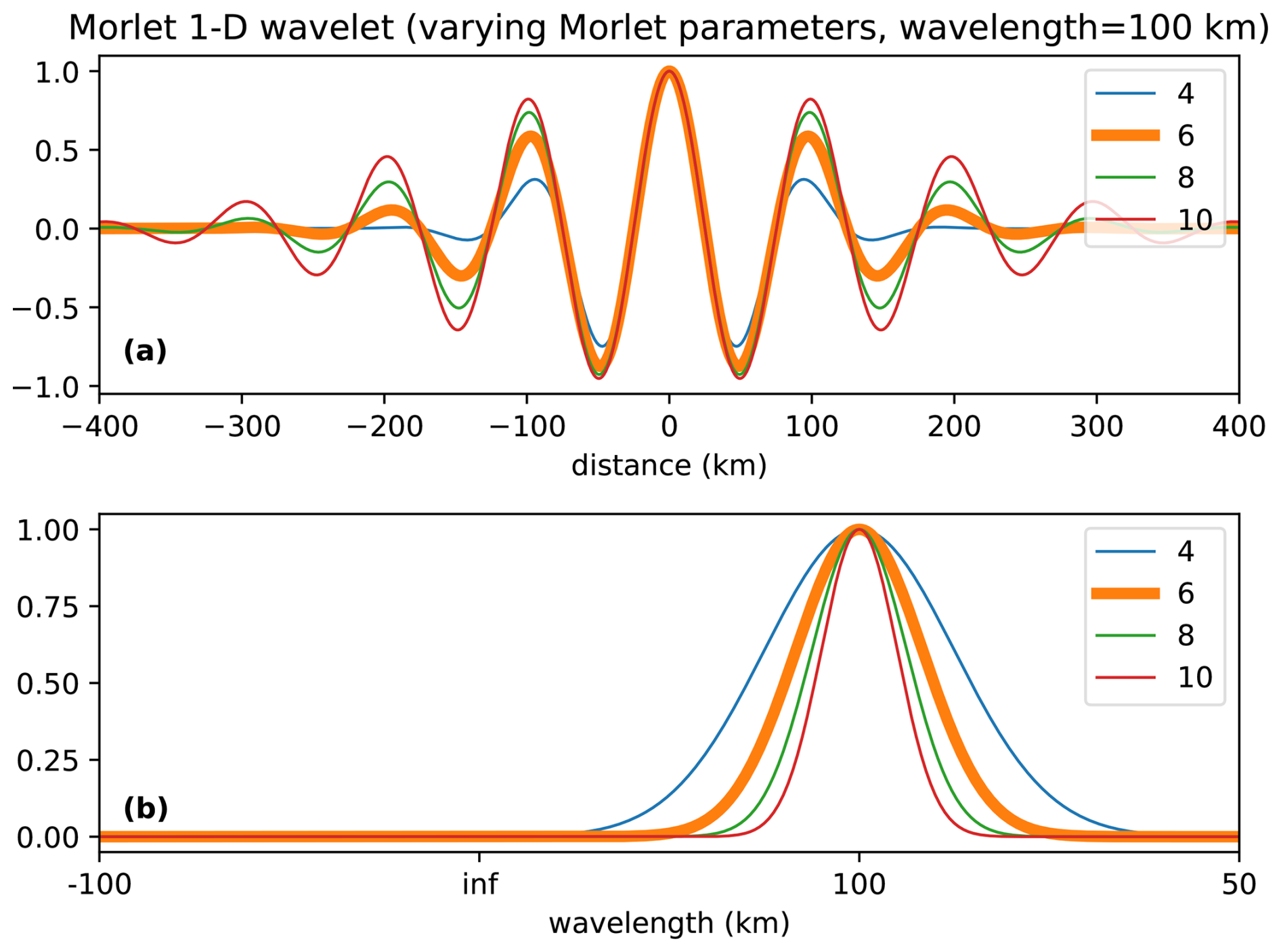
Figure 1 The Morlet wavelet in spatial and frequency space. The Morlet parameter influences the number of wave crests within the envelope and thus the localization in frequency space.

The ST is a variation of the CWT that allows a simpler interpretation of results. The ST S is defined as

$$\begin{array}{}\text{(5)}& \begin{array}{rl}\mathrm{Sf}(u,s)& ={\displaystyle \frac{\sqrt{\mathrm{2}}}{\sqrt{s}\sqrt[\mathrm{4}]{\mathit{\pi }}}}{e}^{-ik\frac{u}{s}}〈f,{\mathit{\psi }}_{u,s}〉\\ & ={\displaystyle \frac{\mathrm{2}}{s\sqrt{\mathrm{2}\mathit{\pi }}}}\underset{-\mathrm{\infty }}{\overset{\mathrm{\infty }}{\int }}f\left(t\right)e^{-\frac{\mathrm{1}}{\mathrm{2}}{\left(\frac{t-u}{s}\right)}^{\mathrm{2}}}{e}^{-ki\frac{t}{s}}\mathrm{d}t,\end{array}\end{array}$$

typically choosing k=2π; there is a difference of a factor of 2 to the definition by Stockwell et al. (1996) as we analyse real-valued in contrast to complex-valued functions. Please note the similarity of this equation to Eq. (1); the differences are the scale-dependent scaling of coefficients and the location-dependent phase correction, which can be seen in the harmonic term. For the CWT the harmonic term is shifted with the u variable causing the coefficients to rotate in phase space when u is varied, whereas it remains fixed in the ST. The discrete ST as originally defined by Stockwell et al. (1996) always uses N dyadic scales for data of length N (effectively using a discretization parameter d_j=1), whereas the given implementation is more flexible. On the continuous side, they are identical.

Both the CWT using the Morlet wavelet and the ST are closely related to the Gabor transform, which is a short-time Fourier transform using a Gaussian window (Gabor, 1946). The notable difference between the Gabor transform and the ST is the wavelength-dependent scaling of the window, which varies for the ST with the scale parameter s, whereas it is of a fixed size for the Gabor transform. This causes the spectral resolution of the Gabor transform to vary for different scales (i.e. it is spectrally highly resolved for high frequencies but spectrally coarsely resolved for low frequencies), whereas the CWT (and its derivative the ST) has a uniform spectral resolution.

The scaling of the CWT by ${\sqrt{s}}^{-\mathrm{1}}$ allows the ST coefficients for k=2π to be directly interpreted as amplitude at wavelength s (Stockwell et al., 1996); the proof of this is rather straightforward and will not be repeated here, as it has no relation to the implementation of the software package. This relationship holds for an input signal containing a harmonic oscillation of infinite extent, whereas for smaller wave packets, a reduction in derived amplitude may occur. The Morlet-parameter can be taken as a rough guideline: if the wave packet has fewer periods than the Morlet parameter, the dampening cannot be neglected. For the ST, these are roughly six full periods.

A similar scheme to the ST was developed by Chen and Chu (2017) lacking the phase correction. Without phase correction, the complex angle of the coefficients varies by 2π while been translated over one wavelength. The JuWavelet code implements the pure CWT, the ST, and also the variation introduced by Chen and Chu (2017) by the name of “scaled” as this variation only scales the coefficients to align with the amplitude of a infinite monochromatic analysed signal. For 1-D a Gabor transform is also available. All relevant transform methods have a mode parameter to select the desired transform; by default, the S transform variation is used, as this delivers the most useful coefficients. Please note that while the normal CWT transforms Gaussian white noise in the input signal to Gaussian white noise in the coefficients, the ST introduces a colouring of the noise due to the scaling of coefficients with scale such that coefficients of small periods are more “noisy” than those of large periods.

Both the implementations of CWT and ST may use any parameter for the Morlet wavelet free parameter k. Practically, this tunes the relationship between spatial and spectral resolution of the transforms. A higher parameter k results in a better spectral resolution at the cost of spatial resolution as the Heisenberg uncertainty relation imposes limits (e.g. Weyl, 1931). Smaller values than 2π cause the wavelet to become “less admissible” as more and more energy leaks into negative frequencies, which invalidates some of the proofs underlying the CWT. Practically, values as small as 5 can be used (Farge, 1992); smaller values would require some modifications to the wavelet (i.e. setting non-positive frequencies to zero) for the reconstruction to work properly and associated correction terms, e.g. in the conversion from scale to period. Several studies have examined the effect of differing trade-offs and configurations, and we refer to these studies for details (e.g. Fritts et al., 1998; Pinnegar and Mansinha, 2003; Hindley et al., 2016, 2019). In the case that a value different from the default k=2π is used, the wavelet scale parameter of the transform and the period (or wavelength) of the associated wave in the analysed signal differ; the decomposition in the code always returns both the scale and the period for all computed coefficients, and the supplied period should be used for almost all purposes. Different k parameters require different constants for the reconstruction, if desired. The code contains pre-computed values C_δ for the most sensible Morlet parameters (i.e. single-digit integers and multiples of π); for other values, it will be computed on the fly and cached for repeated use within the same program execution.

The mathematics for the 2-D and 3-D transforms are extensions of the formulas for the 1-D transform and rather verbose due to the added dimensions. They are thus given in the Appendix A1 and A2, respectively. They do not introduce relevant new concepts aside the one or two angles rotating the wavelet in two or three dimensions, respectively, and the aspect ratio described in the next paragraph.

An additional feature only available for the 2-D and 3-D transforms is the addition of an aspect ratio, which effectively scales the axis of the last dimension before applying the transform, which does not affect or resample the data field. The basis functions of the CWT and ST are defined to be isotropic. If the analysis shall be employed using actual units, e.g. kilometres, this can pose a problem for vertical cross-sections of atmospheric gravity waves, which are often hundreds of times wider than tall and often only have one or two periods. Using a simple 2-D ST will use basis functions, which extend vertically beyond the wave structure and thus cause the derived coefficients to be much smaller than the amplitude of the present waves; i.e. the derived amplitudes are dampened. Scaling the 2-D field vertically such that the measured waves are more “quadratic” or “cubic”, respectively, resolves this issue (an equivalent interpretation of the mathematics would be using a wavelet condensed in one dimension). JuWavelet is capable of scaling the axis of the last dimension by a scalar. This has no effect on the mathematical transform itself; however, the computation of directional wavelengths changes. For this reason, the corresponding directional wavelengths in the two or three dimensions are provided for the higher-order transforms. Generally, the decomposition results vary depending on the units of the employed axis, and a “normalization” of the data to a sensible relationship is useful for a meaningful analysis. Both CWT and ST will always be invertible, but the interpretation of results is simpler if the axes of the data field are scaled in a reasonable fashion; otherwise the derived coefficients will more strongly deviate from the desired local amplitudes.

4 The 2-D decomposition

In this section, we describe the call of the 2-D decomposition as some of its parameters are not very intuitive. The 1-D and 3-D transforms are very similar. The signature of the 2-D transform is as follows:

def decompose2d(
    data, dx, dy, s0, dj, js, jt, aspect=1,
    nxpad=None, nypad=None, opts=None, filt=None,
    mode="stockwell", dtype=np.complex128):

The first parameter data refers to the 2-D NumPy array containing the data to be analysed. It needs to be regularly sampled, and the sampling distances in x and y direction are given by the dx and dy parameters. The 2-D CWT handles the analysis of data defined on an infinite plane. Here, we have a finite set of sampled data, and the implementation assumes that the data are defined as “zero” outside the given samples. If the data are not naturally zero, it is advisable to employ a preprocessing step to subtract an hopefully uninteresting average value, e.g. using an appropriately sized median filter. Another option is a so-called tapering, which surrounds the data with a boundary region in which it is smoothly brought to zero to reduce the effect of ringing in the analysis due to discontinuity that would otherwise be present at the border. A simple tapering function called smooth_edges is contained in the utils submodule.

The aspect parameter effectively scales the dy parameter with the difference that the decomposition returns the directional wavelengths for the correct sampling distance. The provided directional wavelength assumes that the unit of the x and y axis is identical. If they have different units such as length and time, the interpretation is obviously more difficult and cannot be automated. Values of 1 for both dx and dy can be used as well to have a fully unitless analysis.

The CWT is defined for all non-negative scales. For practical reasons, only a finite number of these scales is evaluated by the implementation; the available data field is also necessarily band-limited due to its sampled nature. The s0 parameter defines the smallest scale to be analysed. A value resulting in an analysed period smaller than both 2dx and 2dy will obviously not deliver useful results due to the Nyquist frequency. js defines the number of scales to be analysed. The runtime of the transform increases linearly with the number of analysed scales. Towards the longer scales, values resulting in wavelet basis functions of a size similar to the data set will provide ever more dampened values due to the increasing overlap between analysing wavelet basis function and the zero region around the supplied data. The dj parameter configures the sampling of the scales to be analysed with the formula of $\left\{s_{\mathrm{0}}{\mathrm{2}}^{j{d}_j}|j\in [\mathrm{0},\mathrm{\dots },j_s-\mathrm{1}]\right\}$. A reasonable value for dj is typically $\mathrm{1}/\mathrm{4}$ (Torrence and Compo, 1998), but an exploratory analysis benefits from the speedup of a value of 1 in combination with a smaller js parameter. The jt parameter defines the number of angles to be used in the analysis. The 2-D Morlet wavelet can be rotated by an angle θ with values within the half-open interval of [0,π). A good starting value would be something in the order of 12. More angles allow a better identification of wave parameters, but the runtime increases linearly with the examined angles.

The opts parameter is a Python dictionary allowing us to configure the k parameter of the Morlet wavelet for both the Morlet CWT and ST transform. For example, opts={"param": 5} configures a value of 5, allowing for a better spatial resolution at the cost of spectral resolution in comparison to the default value of 2π.

The filt parameter is a Python dictionary allowing us to skip the computation of selected directional wavelength to speed up the computation. The possible keys vary depending on the employed transform. The 2-D transform supports the keys min_wavelength_x, max_wavelength_x, min_wavelength_y, max_wavelength_y, min_theta, and max_theta. For example filt={"min_wavelength_x": 10, "max_wavelength_x": 100} only computes coefficients associated with directional wavelength along the x axis between 10 and 100. Coefficients associated with wavelengths outside this range will be filled with NaN values.

The padding parameters nxpad and nypad allow us to manually configure the padding necessary to perform the convolution in Fourier space. The underlying fast Fourier transform (FFT) assumes data to be periodic in all spatial directions, which is not an assumption underlying the CWT. To avoid effects of this periodicity affecting the analysis, the data are padded with zeros, applying a different assumption of the data being zero outside the supplied data. If the data are actually periodic, this can be exploited by setting the padding parameters to zero. It should normally be left to its default values, which guarantee correct results, albeit at increased runtime. In the case that the data field is already sufficiently padded with zeros (e.g. due to tapering or similar preprocessing steps), it should be set appropriately to save memory and runtime.

The mode parameter configures the type of transform to be used. The default value of “stockwell” uses the ST, while “cwt” uses the Morlet CWT.

The final parameter dtype defines the numerical format to store the coefficients in. The computation internally uses the double format to reduce error propagation, but the results can be stored in lower accuracy to save memory. The default format is complex128 for the 1-D and 2-D transform and complex64 for the 3-D transform.

5 Examples

This section gives several examples demonstrating the capabilities and application of the available analysis tool.

5.1 1-D analysis on synthetic data

The first example² serves to showcase the ability of the CWT to analyse a signal for individual components and highlight the differences between the implemented method. Figure 2 shows a signal consisting of three subsignals in panel (a). The individual subsignals are shown in panel (e). One subsignal decreases linearly in amplitude, one changes its frequency, and one is only present in the second half, which would be typically time or space in geophysical data. The signal is a 1-D array with 2048 entries (8 kB). We first apply the 1-D CWT to the signal using 𝚍𝚡=1, 𝚜0=2, $\mathtt{\text{dj}}=\mathrm{1}/\mathrm{8}$, 𝚓𝚜=56, and k=2π. Panel (b) shows nicely how the subsignals are reflected in peaks of the magnitude. The phase signal (panel f) is difficult to interpret, as it changes linearly during the signal. Here, as a comparison, we showcase the result of a Gabor short-time Fourier transform (STFT; e.g. Allen, 1977; Mallat, 1999), which has an analysing function using a Gaussian envelope with a fixed standard deviation of length 100. In panels (c) and (g), one can see that the results are similar to the CWT but that the spectral resolution is better for small periods and worse for large periods. This is a direct consequence of the changing number of periods in the basis function due to the envelope of fixed size. Finally, we apply the 1-D ST to the signal using the same parameters as in the 1-D CWT case. Results are shown in panels (d) and (h). The magnitude of the coefficients corresponds to the magnitude of the original signals, as expected. Another difference can be spotted in the phase plot. The phase stays constant in the analysis at the correct period length, which gives another indication of the “correctly” identified period length. Due to evaluating only a discrete set of scales on a computer, one seldom really analyses the correct period and is much more likely to look at one “close” to the correct one, where the phase still changes albeit, slowly. Also, many real-life signals vary slightly in frequency, so this makes the phase difficult to interpret even for the ST.

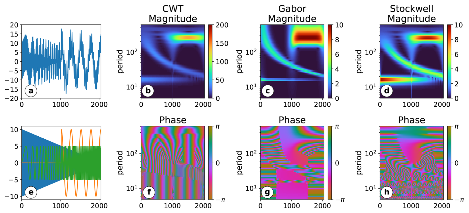
Figure 2 An analysis of a combination of three signals, which each vary in a different quantity (amplitude, frequency, location). Panel (a) shows the assembled signal, while panel (e) shows the individual signals. Panel (b) and (f) show the magnitude and the phase of the CWT coefficients. Panel (c) and (g) show the magnitude and phase of the Gabor STFT coefficients. Panels (d) and (h) show the magnitude and phase of the ST coefficients.

On a more practical note, please observe that the results of the CWT get more “fuzzy” on the edge for larger scales. This is due to the increasing extent of the wavelet basis functions, which extend beyond the original signal, where the algorithm assumes a signal of “zero”. This can cause a variety of artefacts in the coefficients close to the border; here, the magnitude decreases, but for data that are not “zero” at the boundaries, ringing-like artefacts will also appear. To avoid this as much as possible, it is suggested to use tapering, i.e. to bring the signal to zero in a controlled fashion. Be generally aware of this when interpreting the coefficients. Torrence and Compo (1998) provide a “cone of influence” for 1-D data, which can be found in the utils submodule for 1-D decompositions.

5.2 1-D analysis of sea surface temperature (SST)

As a second example³, we would like to reproduce a figure by Torrence and Compo (1998) analysing an actual series of sea surface temperatures (SSTs) as a measure of the amplitude of the El Niño–Southern Oscillation. The software and data used by Torrence and Compo (1998) for this 1-D analysis are readily available (see Acknowledgements). The SST data are a 1-D array with 504 entries (3 kB). We apply our 1-D CWT to the SST time series using the following set of parameters: 𝚍𝚡=0.25, 𝚜0=0.5, $\mathtt{\text{dj}}=\mathrm{1}/\mathrm{4}$, 𝚓𝚜=37, k=6. Results of the analysis are shown in Fig. 3. The SST time series shows obvious “high-frequency” oscillations of short timescales of a few years in addition to less obvious long-term features. The power spectrum (i.e. the squared absolute values of the coefficients of the CWT) is shown in Fig. 3b. The power relates to the variance of the original signal explained by the indicated periods and time frames. Here, the hatched region indicates the coefficients roughly, where the relevant support of the wavelet extends beyond the region of available data (cone of influence). Please note that the CWT of JuWavelet retains the energy of the continuous signal as described in Eq. (3), whereas Torrence and Compo (1998) defined their transform to conserve the variance of the sampled signal, which causes the spectrum to change if the sampling distance varies; this causes a discrepancy of a factor of 4 between their figure and our figure. Panel (c) shows the absolute value of the ST, which directly relates to the amplitude in the original signal. Please note how the ST reduces the coefficient magnitude for longer periods and elevates values for smaller periods (and thus also amplifies noise).

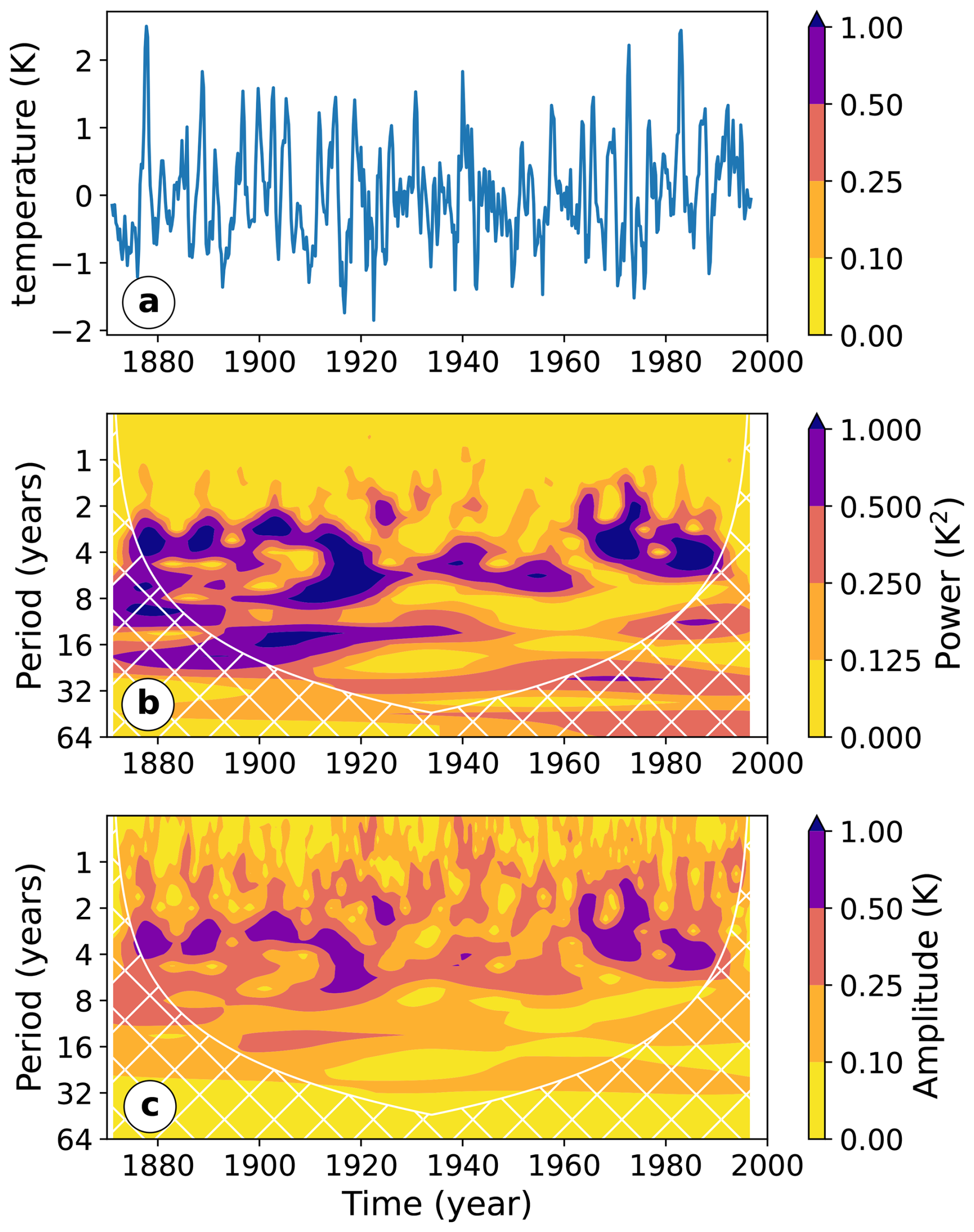
Figure 3 A replication of the analysis of the Niño3 SST index from Torrence and Compo (1998). Panel (a) shows the index itself, while panel (b) shows the power spectrum of the 1-D CWT analysis using a Morlet wavelet (with parameter 2π). The hatched region indicates untrustworthy values where the relevant wavelet support extends over the region where data are available. Panel (c) shows the amplitudes derived from the ST for comparison.

5.3 2-D analysis on synthetic data

The 2-D Morlet wavelet is shown in Fig. 4 for differing scales and angles. It is used to analyse⁴ a synthetic 2-D field containing several wave packets depicted in Fig. 5a. The synthetic field is similarly designed as the synthetic wave field shown in Hindley et al. (2016, therein Fig. 2) and contains eight partially overlapping waves. All waves have an amplitude of 1 but differing envelopes. One example uses a circular pattern similar to gravity waves induced by point sources. The field is an array with 200×200 entries and takes up a disc space of 0.3 MB. The CWT transforms this 2-D field into a 4-D field with added dimensions of scale (or period) and angle. The disc space occupied by the 4-D array increases linearly with the number of scales and rotation angles, and so does the computation time. For the wavelet analysis of the synthetic wave field, we used $\mathtt{\text{dx}}=\mathtt{\text{dy}}=\mathrm{1}$, 𝚜0=2 𝚍𝚡, $\mathtt{\text{dj}}=\mathrm{1}/\mathrm{16}$, 𝚓𝚜=106, 𝚓𝚝=18, k=4, and an aspect ratio of 1, resulting in an array of size 1.4 GB. Please note that due to an ambiguity of π, the 18 angles are equally distributed in the range [0,π]. This 4-D information field is difficult to visualize, so following Hindley et al. (2016) we collapse the 4-D field by selecting the coefficient with the largest amplitude for each spatial sample and selecting the associated wavelength and angle. This gives again 2-D fields. Figure 5b and c show the reconstruction of the dominant modes and the resulting amplitude field, respectively. Please note that we used the scaled version (mode = “scaled”), which yields the correct amplitudes of the signal. While the structure of the wave field is nicely reconstructed, the amplitudes are all strictly smaller than 1, as the relationship between wavelet coefficients and amplitude of original waves only holds for monochromatic waves of infinite extent, and the employed examples are all comparatively small. Here the CWT uses the Morlet parameter of k=4, which is chosen due to the strong localization of the wave packets in space. The wavelength and wavefront orientations associated with the dominant coefficients are depicted in panel (d) and (e). In addition, we oppose input and output wavelengths and wave orientations in Fig. 5f. While wavefront orientations are in perfect agreement, we notice an underestimation of the wavelength for wave packet 6 and 7. The reason for this underestimation might be their large wavelengths in comparison to the physical extent of their envelopes. Another contributing factor might be the vicinity of wave packets 6 and 7 to the boundary of the domain.

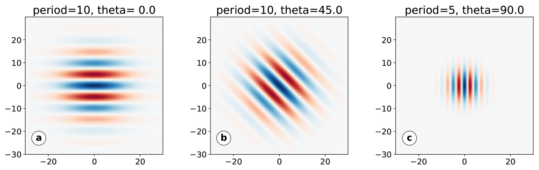
Figure 4 The 2-D Morlet wavelet. The three panels showcase variations when changing the rotation or the scale parameter.

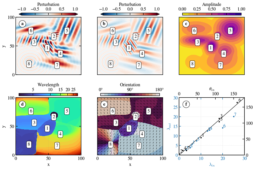
Figure 5 An example of a 2-D CWT analysis. Panel (a) shows the synthetic field containing several waves. A CWT analyses this field and the “dominant” wavelet; i.e. the wavelet with the largest coefficient is identified for each spatial sample. Panel (b) shows the reconstruction of the dominant mode, panel (c) the resulting amplitude, panel (d) the corresponding wavelength, panel (e) the corresponding orientation. Panel (f) opposes input wavelength and orientation to estimated quantities.

5.4 2-D reconstruction

The supplied code can not only compute the decomposition but also reconstruct the original field from the CWT. This allows the manipulation of coefficients for a wide variety of purposes. Figure 6 shows several examples⁵ thereof. Please note that the physical dimensions of the data are widely different. While vertically, the measured data cover about 50 km, horizontally about a thousand are covered. Also the gravity waves in the data often have much larger horizontal than vertical wavelengths. To facilitate the analysis here, we make use of the aspect feature described above. Here, an aspect of 40 was employed, which delivered reasonable results and did not leave the computed coefficients for most angles empty (as is the case for the default aspect of 1).

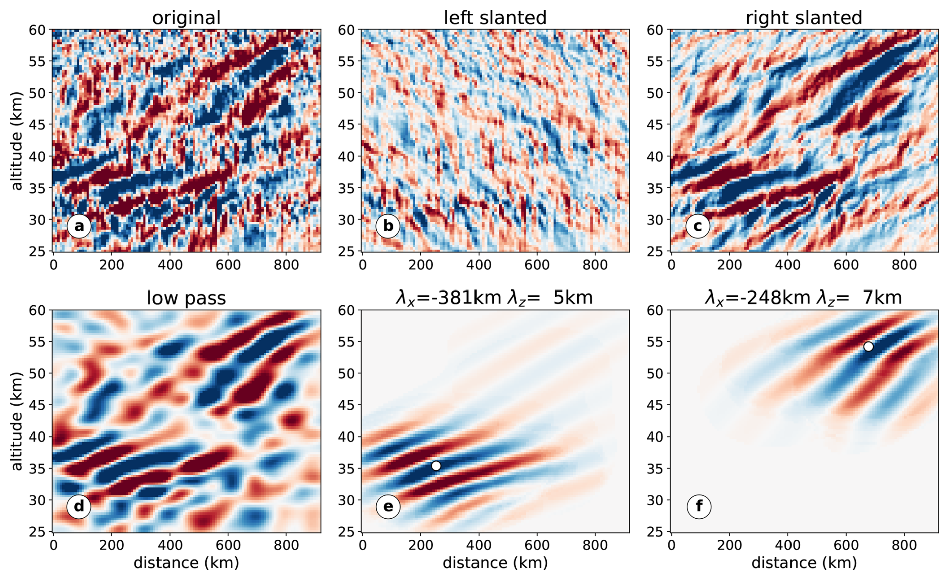
Figure 6 This example shows the capabilities of reconstructing a data set from a modified set of coefficients. Panel (a) shows the original data field. Panel (b) shows a filtered reconstruction allowing only left slanted waves, while panel (c) shows the right slanted waves. The sum of (b) and (c) gives the original data. Panel (d) shows the effect of discarding the small scales, effectively a low pass. Panels (e) and (f) show reconstructions containing only coefficients from the vicinity of two local maxima in the CWT corresponding to two wave packets, which can be identified in this manner with wavelengths of 381 km horizontally and 5.5 km vertically for panel (e) and 248 km horizontally and 7.4 km vertically for panel (f). The spatial location of the coefficient with the largest amplitude is given by a white circle.

The data set is a down-sampled version of the temperature data measured by the ALIMA lidar (Kaifler et al., 2017) analysed and discussed by Geldenhuys et al. (2023) using an earlier version of this software. The temperature field (see Fig. 6a) is a 2-D array with 89 × 110 entries (244 kB). We apply the 2-D CWT to the data using the following parameters: 𝚍𝚡=8.46, 𝚍𝚢=0.4, 𝚜0=20, $\mathtt{\text{dj}}=\mathrm{1}/\mathrm{45}$, 𝚓𝚜=20, 𝚓𝚝=18, 𝚊𝚜𝚙𝚎𝚌𝚝=40, and k=2π. The coefficients provided by the CWT can be filtered; i.e. practically “undesired” coefficients are set to zero before performing a reconstruction. In this manner one can filter out components according to angle and thus separate the original field into left-slanted (Fig. 6b) or right-slanted waves (Fig. 6c), which likely also correspond here to a downward or upward propagation direction, respectively. A low-pass filter can be finely configured by setting wavelet coefficients to 0 where periods are smaller than 100 km (Fig. 6d) or vice versa. It is also possible to extract individual wave packets. A simple clustering algorithm contained in the software package identifies different wave packets and the associated CWT coefficients. Due to the finite spectral and spatial resolution of the employed basis, the basis function closest in parameters to the true wave packet will typically have the largest coefficient, but spectrally neighbouring basis functions will still have large values decreasing with “distance” in the wavelet space. Including these in the reconstruction is important to retain the amplitude of the packet. The algorithm assumes that overlapping wave packets are separable in spectral space by coefficients below a configurable threshold. Due to the high dimensionality of the CWT coefficients, this is a reasonable assumption. The algorithm then identifies the largest coefficient not part of an identified cluster and first identifies the scales and angles associated with this cluster by looking for neighbouring scales and angles at this point above the threshold. In a second step, the spatial extent is explored in the same way, starting from the identified scales and angles. The algorithm repeats until no further cluster can be constructed from remaining coefficients. By only using the coefficients of a single cluster in the reconstruction, individual wave packets can be identified and analysed with respect to wavelength, direction, and amplitude. The two major features of the field are given in Fig. 6e and f. The directional wavelengths given in the panel headings fit the observable structure close to the highlighted centre of the wave packet well. Further away, the agreement is worse; here the supplied automatic clustering algorithm is unable to identify properly the cluster boundaries. We suggest mostly using the automatic algorithm for exploratory analysis.

5.5 2-D separation of two waves

In general, waves can overlap. However, most studies focus on analysing wave parameters with dominant amplitudes at spatial samples (such as done in Sect. 5.3; see also Hindley et al., 2016, 2019; Wright et al., 2021). In this example⁶, we present a superposition of a simple large-scale plane wave and a small-scale Kelvin wake pattern. Figure 7a shows the wave field with 640×480 entries (1.2 MB). We compute the 2-D CWT of the wave field using $\mathtt{\text{dx}}=\mathtt{\text{dy}}=\mathrm{0.1}$ km, 𝚜0=2𝚍𝚡, $\mathtt{\text{dj}}=\mathrm{1}/\mathrm{8}$, 𝚓𝚜=58, 𝚓𝚝=9, k=4, and an aspect ratio of 1 and obtain a 4-D array of wavelet coefficients (memory space: 2.8 GB, runtime: 2.8 min (two physical cores, i.e. four logical CPUs via two-way hyperthreading)). Subsequently, we use the watershed function from the skimage.segmentation package in Python to label the wavelet coefficients. For this, we calculate the power spectrum and invert it. The watershed function then segments regions in the spectrum that are separated by a minimum. In this example we find two major segments that are associated with the small- and the large-scale wave. To reconstruct the small-scale wave, all wavelet coefficients corresponding to the large-scale wave are set to zero and vice versa. The reconstruction of the small- and large-scale wave is shown in Fig. 7b, and c. To represent the respective amplitudes, wavelengths, and orientations, we take the adjusted wavelet coefficients and collapse the modified 4-D array of coefficients by saving the parameters that are associated with the amplitude maximum at each spatial sample. The result is shown in Fig. 7d–i. In contrast to the example in Sect. 5.3 the two wave fields in this example cannot be separated by simply looking for dominant amplitudes, but we must make use of their different scales. Here, we find that the watershed function nicely separates the two waves. Not only the wave fields can be reconstructed separately, but also the wave's spectral properties such as amplitude, wavelength, and orientation can be studied separately. Please note that the retrieved large-scale wave amplitude is weaker at the boundary of the domain due to the enhanced overlap of the 2-D wavelet with padded zeros outside the domain. We apply the same watershed function to the wavelet power spectrum from Sect. 5.3 and reconstruct almost all synthetic wave packets separately (see Fig. A1). Only the location, scales and orientations of wave packets 4 and 7 are to similar, and hence these two wave packets cannot be separated by the algorithm (see Fig. A1b). These examples demonstrate the power of combining the 2-D CWT with an appropriate segmentation algorithm.

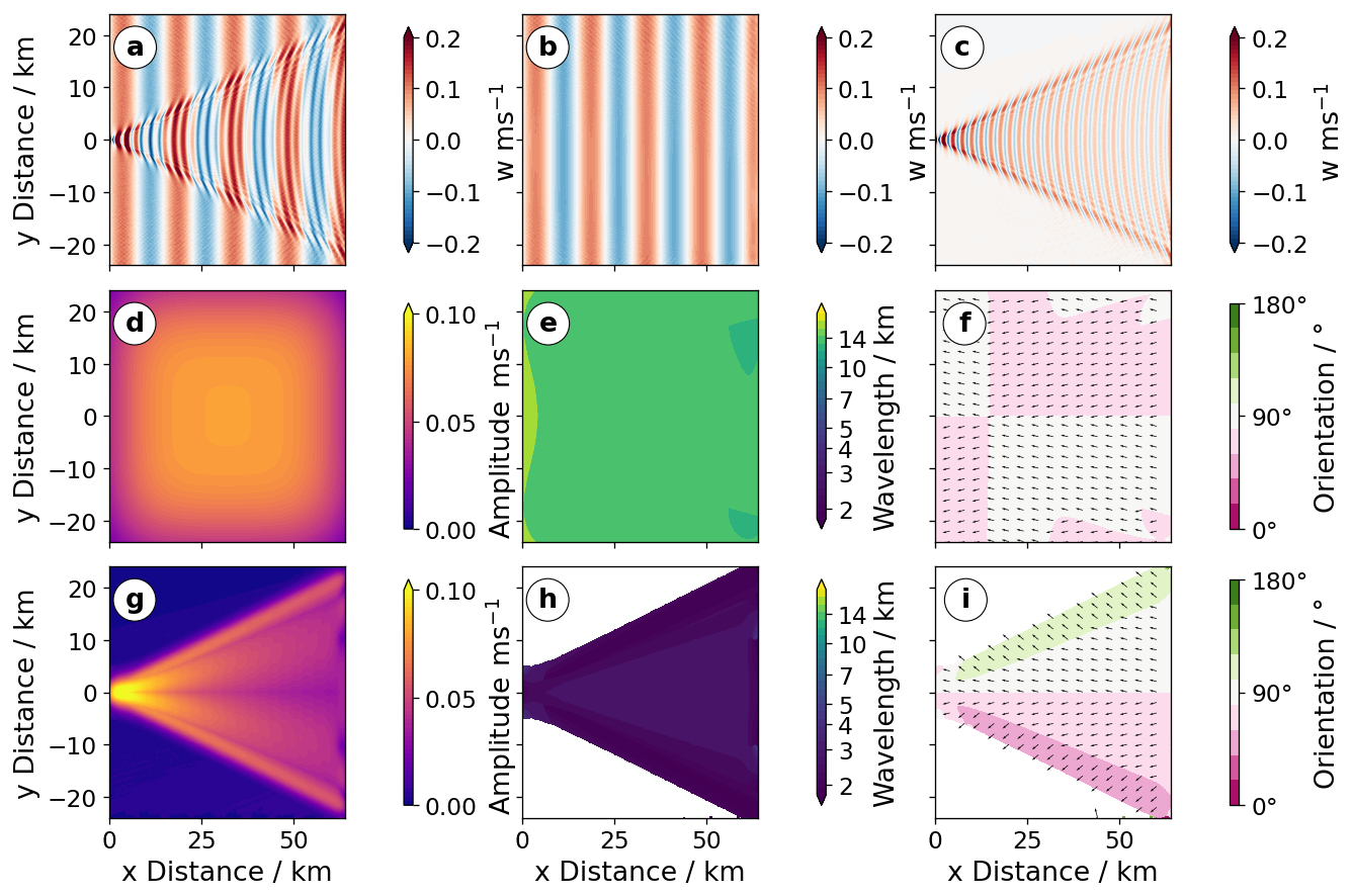
Figure 7 This example shows the capabilities of reconstructing a data set from a modified set of coefficients. Panel (a) shows a simulated superposition of two waves, one of large scale and one of small scale. Panels (b) and (c) show filtered reconstructions of the large-scale and small-scale waves. The sum of (b) and (c) gives the original data. Panels (d), (e), and (f) show the amplitude, wavelength, and orientation of the large-scale wave. Panels (g), (h), and (i) show the amplitude, wavelength, and orientation of the small-scale wave.

5.6 3-D analysis of synthetic data

Figure 8 shows the 3-D structure of a mountain wave. For this example⁷ we compute the vertical displacement (see Eq. 20 in Smith, 1980) given a bell-shaped mountain (h=1 000 m, a=25 000 m) as well as a static stability of $N=\mathrm{0.02}{\mathrm{s}}^{-\mathrm{1}}$ and a horizontal wind speed of $u=\mathrm{10}{\mathrm{ms}}^{-\mathrm{1}}$. The data are a 3-D array with $\mathrm{250}\times \mathrm{300}\times \mathrm{40}$ entries (11.4 MB). The 3-D CWT is applied to the wave field using the following parameters: $\mathtt{\text{dx}}=\mathtt{\text{dy}}=\mathrm{2}$ km, 𝚍𝚣=0.25 km, 𝚜0=4 km, $\mathtt{\text{dj}}=\mathrm{1}/\mathrm{4}$, 𝚓𝚜=16, 𝚓𝚝=6, 𝚓𝚙=7, k=4, and an aspect ratio of 10. As a result of the 3-D CWT we get a 6-D object containing wavelet coefficients for all three spatial, one scale, and two angle dimensions (memory space: 13.5 GB, runtime: 0.74 h (16 physical cores, i.e. 32 logical CPUs via two-way hyperthreading)). In order to illustrate the amplitude of the wave field, we collapse the 6-D CWT into a 3-D object containing the maximum amplitude for each spatial sample. We then choose to illustrate the isosurface connected to an amplitude of 70 m of vertical displacement. The structure of the amplitude isosurface agrees nicely with the 3-D wave field in the left panel.

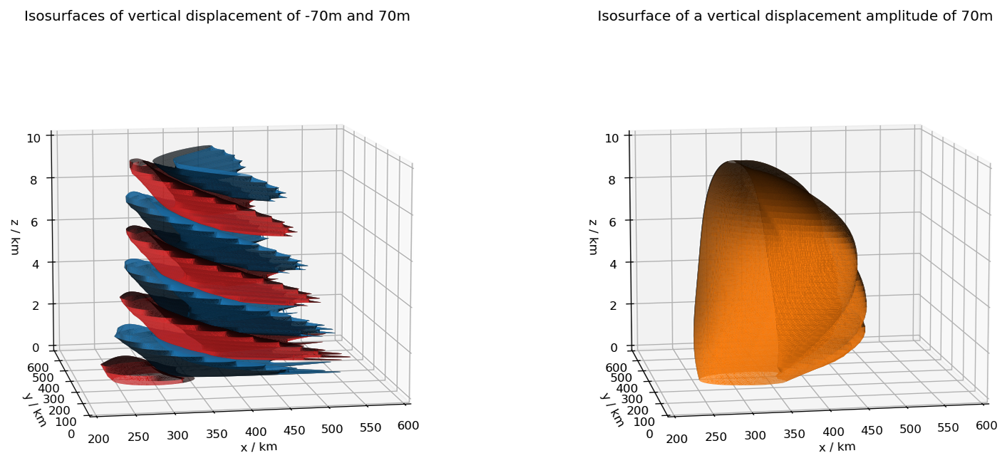
Figure 8 An example of a 3-D CWT analysis. The left panel shows a modelled mountain wave field following Smith (1980). Isosurfaces are drawn for $\mathit{\eta }=\pm \mathrm{70}$ m. A CWT analyses this field and the “dominant” wavelet; i.e. the wavelet with the largest coefficient is identified for each spatial sample. The right panel shows the isosurface for an amplitude of 70 m.

6 Implementation

The sampling of the CWT draws heavily on the fast Fourier transform (FFT). We effectively discretize Eq. (2) and use the FFT to compute $\widehat{f}$ and the inverse continuous Fourier transform. This computes the CWT for all sampled values of u (corresponding to the sampling of the supplied data set) and one scale. Effectively, one FFT is needed for each scale, which largely determines the computational complexity.

The software package is available in the Python programming language. It leverages the NumPy library heavily for its computational needs. For the 1-D transform, let n_s be the number of scales and n_x the length of data. One FFT is needed for analysing the data and n_s FFTs for computing the coefficients. Then the 1-D transform is of complexity O(n_sn_xlog n_x) neglecting constants and smaller terms⁸. With n_y and n_z and n_θ and n_ϕ the length of higher dimensions and number of analysed angles, respectively, the complexity of the 2-D transform can be estimated to be O(n_sn_θn_xn_ylog (n_xn_y)), and the 3-D transform is in the order of O(n_sn_θn_ϕn_xn_yn_zlog (n_xn_yn_z)), again depending on the number of 2-D and 3-D higher-dimensional FFT evaluations.

As almost all computation time is spent doing FFTs, support for both the Intel Math kernel library and the FFTW library (Frigo and Johnson, 2005) is available, which provide highly optimized and parallelized implementations thereof. This requires the mkl_fft or pyFFTW Python package, respectively. By default, JuWavelet first tries MKL and then FFTW, but the employed routines can also be configured during runtime using the functions of the fft submodule. Further parallelization, in particular over multiple nodes of a supercomputer, can be realized by distributing individual scales onto different processes and/or machines or using selective filters and aggregating the results.

7 Conclusions

The presented software package closes a gap by providing readily available 1-D, 2-D, and 3-D STs and Morlet CWTs. Both analysis and reconstruction formulas are implemented such that the filtering of signals for individual wave packets is also possible. The software has been used successfully for the published analysis of temperature measurements but is well suited for the analysis of other localized wavelike phenomena in geophysics.

Appendix A: Mathematical description of 2-D and 3-D transforms

A1 2-D

The definition for the 2-D Morlet wavelet in Fourier space is

$${\widehat{\mathit{\psi }}}_{s,\mathit{\theta }}({\mathit{\omega }}_x,{\mathit{\omega }}_y)=\mathrm{2}\sqrt{\mathit{\pi }}s{e}^{-\frac{\mathrm{1}}{\mathrm{2}}\left({\left(\mathrm{2}\mathit{\pi }s{\mathit{\omega }}_x-k\cos \left(\mathit{\theta }\right)\right)}^{\mathrm{2}}+{\left(\mathrm{2}\mathit{\pi }s{\mathit{\omega }}_y-k\sin \left(\mathit{\theta }\right)\right)}^{\mathrm{2}}\right)},$$

with $\mathit{\theta }\in [\mathrm{0},\mathit{\pi }]$ denoting the angle of the wavelet. The transform is given by

$$\begin{array}{rl}Wf(u,v,s,\mathit{\theta })& =\underset{-\mathrm{\infty }}{\overset{\mathrm{\infty }}{\int }}\underset{-\mathrm{\infty }}{\overset{\mathrm{\infty }}{\int }}\widehat{f}({\mathit{\omega }}_x,{\mathit{\omega }}_y)s{\left[\widehat{\mathit{\psi }}(s{\mathit{\omega }}_x,s{\mathit{\omega }}_y)\right]}^{*}\\ & \cdot e^{i\mathrm{2}\mathit{\pi }{\mathit{\omega }}_{x}u}{e}^{i\mathrm{2}\mathit{\pi }{\mathit{\omega }}_{y}v}\mathrm{d}{\mathit{\omega }}_x\mathrm{d}{\mathit{\omega }}_y.\end{array}$$

With the same discretization of s as in the 1-D case, and a regular sampling of θ in $\frac{\mathit{\pi }}{j_t}$ steps, the reconstruction formula is

$$f(x,y)\approx {\displaystyle \frac{\mathrm{1}}{C_{\mathit{\delta }}}}\sum _{j=\mathrm{0}}^{j_s-\mathrm{1}}\sum _{k=\mathrm{0}}^{j_t-\mathrm{1}}{\displaystyle \frac{\mathit{\pi }}{j_t}}\mathrm{Re}\left(Wf\left(x,y,s_{\mathrm{0}}{\mathrm{2}}^{j{d}_j},{\displaystyle \frac{k\mathit{\pi }}{j_t}}\right)\right){\displaystyle \frac{d_j\ln \mathrm{2}}{s_{\mathrm{0}}{\mathrm{2}}^{j{d}_j}}}$$

with

$$\begin{array}{rl}& C_{\mathit{\delta }}\approx {\displaystyle \frac{\mathit{\pi }}{j_t}}{d}_j\ln \mathrm{2}\sum _{j=\mathrm{0}}^{j_s-\mathrm{1}}\sum _{k=\mathrm{0}}^{j_t-\mathrm{1}}\mathrm{Re}(\\ & \underset{-\mathrm{\infty }}{\overset{\mathrm{\infty }}{\int }}\underset{-\mathrm{\infty }}{\overset{\mathrm{\infty }}{\int }}{\left[\widehat{\mathit{\psi }}(s_{\mathrm{0}}{\mathrm{2}}^{j{d}_j}{\mathit{\omega }}_x,s_{\mathrm{0}}{\mathrm{2}}^{j{d}_j}{\mathit{\omega }}_y)\right]}^{*}\mathrm{d}{\mathit{\omega }}_x\mathrm{d}{\mathit{\omega }}_y).\end{array}$$

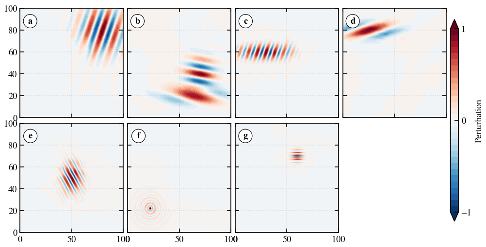
Figure A1 Reconstruction of individual wave packets from the synthetic wave field from Sect. 5.3. Mapping of panels and wave packets is as follows: (a) shows wave packet 5, (b) shows wave packets 4 and 7, (c) shows wave packet 3, (d) shows wave packet 6, (e) shows wave packet 1, (f) shows wave packet 8, and (g) shows wave packet 2.

A2 3-D

The definition for the 3-D Morlet wavelet in Fourier space is

$$\begin{array}{rl}& {\widehat{\mathit{\psi }}}_{s,\mathit{\theta },\mathit{\varphi }}({\mathit{\omega }}_x,{\mathit{\omega }}_y,{\mathit{\omega }}_z)={\displaystyle \frac{{\sqrt{\mathrm{2}}}^{\mathrm{3}}\mathit{\pi }}{\sqrt[\mathrm{4}]{\mathit{\pi }}}}{s}^{\mathrm{3}/\mathrm{2}}\\ & \cdot e^{-\frac{\mathrm{1}}{\mathrm{2}}\left({\left(\mathrm{2}\mathit{\pi }s{\mathit{\omega }}_x-k\cos \left(\mathit{\varphi }\right)\cos \left(\mathit{\theta }\right)\right)}^{\mathrm{2}}+{\left(\mathrm{2}\mathit{\pi }s{\mathit{\omega }}_y-k\cos \left(\mathit{\varphi }\right)\sin \left(\mathit{\theta }\right)\right)}^{\mathrm{2}}+{\left(\mathrm{2}\mathit{\pi }s{\mathit{\omega }}_z-k\sin \left(\mathit{\varphi }\right)\right)}^{\mathrm{2}}\right)}\end{array},$$

with $\mathit{\theta }\in [\mathrm{0},\mathit{\pi }]$ denoting the horizontal turning (azimuth angle) of the wavelet and $\mathit{\varphi }\in [-\mathit{\pi }/\mathrm{2},\mathit{\pi }/\mathrm{2}]$ the vertical rotation (zenith angle). The transform is given by

$$\begin{array}{rl}& Wf(u,v,w,s,\mathit{\theta },\mathit{\varphi })=\underset{-\mathrm{\infty }}{\overset{\mathrm{\infty }}{\int }}\underset{-\mathrm{\infty }}{\overset{\mathrm{\infty }}{\int }}\underset{-\mathrm{\infty }}{\overset{\mathrm{\infty }}{\int }}\widehat{f}({\mathit{\omega }}_x,{\mathit{\omega }}_y,{\mathit{\omega }}_z)s^{\mathrm{3}/\mathrm{2}}\\ & \cdot {\left[\widehat{\mathit{\psi }}(s{\mathit{\omega }}_x,s{\mathit{\omega }}_y,s{\mathit{\omega }}_z)\right]}^{*}{e}^{i\mathrm{2}\mathit{\pi }{\mathit{\omega }}_{x}u}{e}^{i\mathrm{2}\mathit{\pi }{\mathit{\omega }}_{y}v}{e}^{i\mathrm{2}\mathit{\pi }{\mathit{\omega }}_{z}w}\mathrm{d}{\mathit{\omega }}_x\mathrm{d}{\mathit{\omega }}_y\mathrm{d}{\mathit{\omega }}_z.\end{array}$$

With the same discretization of s as in the 1-D case, and a regular sampling of θ and ϕ, the reconstruction formula is

$$\begin{array}{rl}& f(x,y,z)\approx {\displaystyle \frac{\mathrm{1}}{C_{\mathit{\delta }}}}\sum _{j=\mathrm{0}}^{j_s-\mathrm{1}}\sum _{k=\mathrm{0}}^{j_t-\mathrm{1}}\sum _{l=\mathrm{0}}^{j_p-\mathrm{1}}{\displaystyle \frac{\mathit{\pi }}{j_s}}{\displaystyle \frac{\mathit{\pi }}{j_p}}\cos \left({\displaystyle \frac{(l+\mathrm{0.5})\mathit{\pi }}{j_p}}-{\displaystyle \frac{\mathit{\pi }}{\mathrm{2}}}\right)\\ & \cdot \mathrm{Re}\left(Wf\left(x,y,z,s_{\mathrm{0}}{\mathrm{2}}^{j{d}_j},{\displaystyle \frac{k\mathit{\pi }}{j_s}},{\displaystyle \frac{(l+\mathrm{0.5})\mathit{\pi }}{j_p}}-{\displaystyle \frac{\mathit{\pi }}{\mathrm{2}}}\right){\displaystyle \frac{d_j\ln \mathrm{2}}{(s_{\mathrm{0}}{\mathrm{2}}^{j{d}_j}{)}^{\mathrm{3}/\mathrm{2}}}}\right).\end{array}$$

Please note the factor of cos (ϕ) necessary for integrating the rotation over the unit sphere. The sampling of ϕ is shifted by half a sample to avoid the value of $-\mathit{\pi }/\mathrm{2}$ and $\mathit{\pi }/\mathrm{2}$ where the coefficients do not contribute to the reconstruction and the value of θ has no effect on the wavelet. The factor C_δ can be computed as

$$\begin{array}{rl}& C_{\mathit{\delta }}\approx {\displaystyle \frac{\mathit{\pi }}{j_s}}{\displaystyle \frac{\mathit{\pi }}{j_p}}{d}_j\ln \mathrm{2}\sum _{j=\mathrm{0}}^{j_s-\mathrm{1}}\sum _{k=\mathrm{0}}^{j_s-\mathrm{1}}\sum _{l=\mathrm{0}}^{j_p-\mathrm{1}}\cos \left({\displaystyle \frac{(l+\mathrm{0.5})\mathit{\pi }}{j_p}}-{\displaystyle \frac{\mathit{\pi }}{\mathrm{2}}}\right)\\ & \cdot \mathrm{Re}\left(\underset{-\mathrm{\infty }}{\overset{\mathrm{\infty }}{\int }}\underset{-\mathrm{\infty }}{\overset{\mathrm{\infty }}{\int }}\underset{-\mathrm{\infty }}{\overset{\mathrm{\infty }}{\int }}{\left[\widehat{\mathit{\psi }}(s_{\mathrm{0}}{\mathrm{2}}^{j{d}_j}{\mathit{\omega }}_x,s_{\mathrm{0}}{\mathrm{2}}^{j{d}_j}{\mathit{\omega }}_y,s_{\mathrm{0}}{\mathrm{2}}^{j{d}_j}{\mathit{\omega }}_z)\right]}^{*}\mathrm{d}{\mathit{\omega }}_x\mathrm{d}{\mathit{\omega }}_y\mathrm{d}{\mathit{\omega }}_z\right).\end{array}$$