A Python interface to the Fortran-based Parallel Data Assimilation Framework: pyPDAF v1.0.2

Data assimilation (DA) is an essential component of numerical weather and climate prediction. Efficient implementation of DA algorithms benefits both research and operational prediction. Currently, a variety of DA software programs are available. One of the notable DA libraries is the Parallel Data Assimilation Framework (PDAF) designed for ensemble data assimilation. The DA framework is widely used with complex high-dimensional climate models, and is applied for research on atmosphere, ocean, sea ice and marine ecosystem modelling, as well as operational ocean forecasting. Meanwhile, there are increasing demands for flexible and efficient DA implementations using Python due to the increasing amount of intermediate complexity models as well as machine learning based models coded in Python. To accommodate for such demands, we introduce a Python interface to PDAF, pyPDAF. pyPDAF allows for flexible DA system development while retaining the efficient implementation of the core DA algorithms in the Fortran-based PDAF. The ideal use-case of pyPDAF is a DA system where the model integration is independent from the DA program, which reads the model forecast ensemble, produces an analysis, and updates the restart files of the model, or a DA system where the model can be used in Python. With implementations of both PDAF and pyPDAF, this study demonstrates the use of pyPDAF and PDAF in a coupled data assimilation (CDA) setup in a coupled atmosphere-ocean model, the Modular Arbitrary-Order Ocean-Atmosphere Model (MAOOAM). This study demonstrates that pyPDAF allows for PDAF functionalities from Python where users can utilise Python functions to handle case-specific information from observations and numerical model. The study also shows that pyPDAF can be used with high-dimensional systems with little slow-down per analysis step of only up to 13 % for the localized ensemble Kalman filter LETKF in the example used in this study. The study also shows that, compared to PDAF, the overhead of pyPDAF is comparatively smaller when computationally intensive components dominate the DA system. This can be the case for systems with high-dimensional state vectors.

1 Introduction

Data assimilation (DA) combines simulations and observations using dynamical systems theory and statistical methods. This process provides optimal estimates (i.e., analyses), enables parameter estimation, and allows for the evaluation of observation networks. Due to the limited predictability and imperfect models, DA has become one of the most important techniques for numerical weather and climate predictions. Progress of the DA methodology development can be found in various review articles and books (e.g., Bannister, 2017; Carrassi et al., 2018; Vetra-Carvalho et al., 2018; Evensen et al., 2022).

To ameliorate the difficulties in the implementation of different DA approaches, several DA software programs and libraries have been proposed (e.g., Nerger et al., 2005; Anderson et al., 2009; Raanes et al., 2024; Trémolet and Auligne, 2020). Even though the implementation of the core DA algorithms is similar, these software programs/libraries are typically tailored to different purposes. For example, the Joint Effort for Data assimilation Integration (JEDI, Trémolet and Auligne, 2020) is a piece of self-contained software that includes a variety of functionalities that can be used for all aspects of a DA system mainly for operational purposes while DA software for methodology research such as Data Assimilation with Python: a Package for Experimental Research (DAPPER,  Raanes et al., 2024) is designed for identical twin experiments equipped with low complexity models.

One widely used DA framework is the Parallel Data Assimilation Framework (PDAF) developed and maintained by the Alfred Wegener Institute (Nerger et al., 2005; Nerger and Hiller, 2013b). The framework is designed for efficient implementation of ensemble-based DA systems for complex weather and climate models but is also used for research on DA methods with low-dimensional “toy” models. In this generic framework, DA methods accommodate case-specific information about the DA system through functions provided by users including the model fields, treatment of observations, and localisation. These functions are referred to as user-supplied functions. More than 100 studies have used PDAF, including atmosphere (e.g., Shao and Nerger, 2024), ocean (e.g., Losa et al., 2012; Pohlmann et al., 2023), sea ice (e.g., Williams et al., 2023; Zhao et al., 2024), land surface (e.g., Strebel et al., 2022; Kurtz et al., 2016), hydrology (e.g., Tang et al., 2024; Döll et al., 2024), and coupled systems (e.g., AWI-CM in Nerger et al., 2020). Further use-cases of PDAF can be found in the PDAF website (PDAF, 2024). Even though PDAF provides highly optimised DA algorithms, the flexible framework relies on the user-supplied functions to couple DA with model system and observations. The implementation of user-supplied functions still require additional code development, which can be time-consuming especially when the routines have to be written in Fortran, a popular programming language for weather and climate applications.

In recent years, Python is gaining popularity in weather and climate communities due to its flexibility and ease of implementation. For example, Python is adopted by some low- to intermediate-complexity models (e.g., De Cruz et al., 2016; Abernathey et al., 2022), models with a Python wrapper (e.g., McGibbon et al., 2021), and machine learning based models (e.g., Kurth et al., 2023; Lam et al., 2023; Bi et al., 2023). For the application of DA in Python, DAPPER provides a variety of DA algorithms for twin experiments using low-dimensional Python models. The Ensemble and Assimilation Tool, EAT (Bruggeman et al., 2024), which is a wrapper to a Fortran data assimilation system based on PDAF, was proposed to set up a 1D ocean-biogeochemical DA system including the 1D ocean-biogeochemical model, GOTM-FABM. There are also Python packages designed mainly for pedagogical purposes in low-dimensional systems such as openDA (Ahmed et al., 2020) and filterpy (filterpy PyPI, 2024). For high-dimensional applications, there are efficient implementations of DA packages such as HIPPYlib by Villa et al. (2021) and ADAO (SALOME, 2024), but HIPPYlib does not have a focus on ensemble data assimilation approaches whereas ADAO provides various ensemble DA methodologies but it has no support for the localisation used in weather and climate applications. More recently, NEDAS (Ying, 2024) was introduced for offline ensemble DA in climate applications but it currently only supports limited DA algorithms.

Targeted at applications to high-dimensional ensemble data assimilation systems, here, we introduce a Python interface to PDAF, pyPDAF. Using pyPDAF, one can implement both offline and online DA systems using Python. For offline DA systems, DA is performed utilising files written onto a disk, e.g., model restart files. If a numerical model is available in Python, pyPDAF allows for implementing an online DA system where DA algorithms can be used with the Python model with in-memory data exchange that does not need I/O operations bringing about more efficiency than an offline system. Compared to user-supplied functions implemented in Fortran, the Python implementation can facilitate easier code development thanks to a variety of packages readily available in Python. In the meantime, DA algorithms provided by PDAF that are efficiently implemented in Fortran can still be utilised.

In this study, we introduce the design, implementation and functionalities of pyPDAF. Further, in comparison to the existing PDAF implementation, we provide a use-case of pyPDAF in a coupled data assimilation (CDA) setup with the Modular Arbitrary-Order Ocean-Atmosphere Model (MAOOAM, De Cruz et al., 2016) where an arbitrary number of grid points can be specified without changing the model dynamics making it suitable to provide benchmarks of pyPDAF. This use-case allows us to further compare the ease of implementation of pyPDAF with PDAF, and investigate the computational performance under different choices of state vector including both the strongly CDA (SCDA) and weakly CDA (WCDA) cases. In the SCDA case, the atmosphere and ocean are coupled in both forecast and analysis steps. In the WCDA case, the forecast step is coupled but the analysis of the atmosphere and ocean is performed independently.

Here, Sect. 2 will introduce PDAF, the implementation and design of pyPDAF, and the implementation of a DA system in pyPDAF. In Sect. 3, the experimental and model setup will be described. Section 4 will report the performance of PDAF and pyPDAF in the CDA setup. We will conclude in Sect. 5.

2 PDAF and PyPDAF

PDAF is designed for research and operational DA systems. As a Python interface to PDAF, pyPDAF inherits the DA algorithms implemented in PDAF and the same implementation approach to build a DA system.

2.1 Parallel Data Assimilation Framework (PDAF)

PDAF is a Fortran-based DA framework providing fully optimised, parallelised ensemble-based DA algorithms. The framework provides a software library and defines a suite of workflows based on different DA algorithms provided by PDAF. The DA algorithms provided by PDAF will be given in Sect. 2.2.

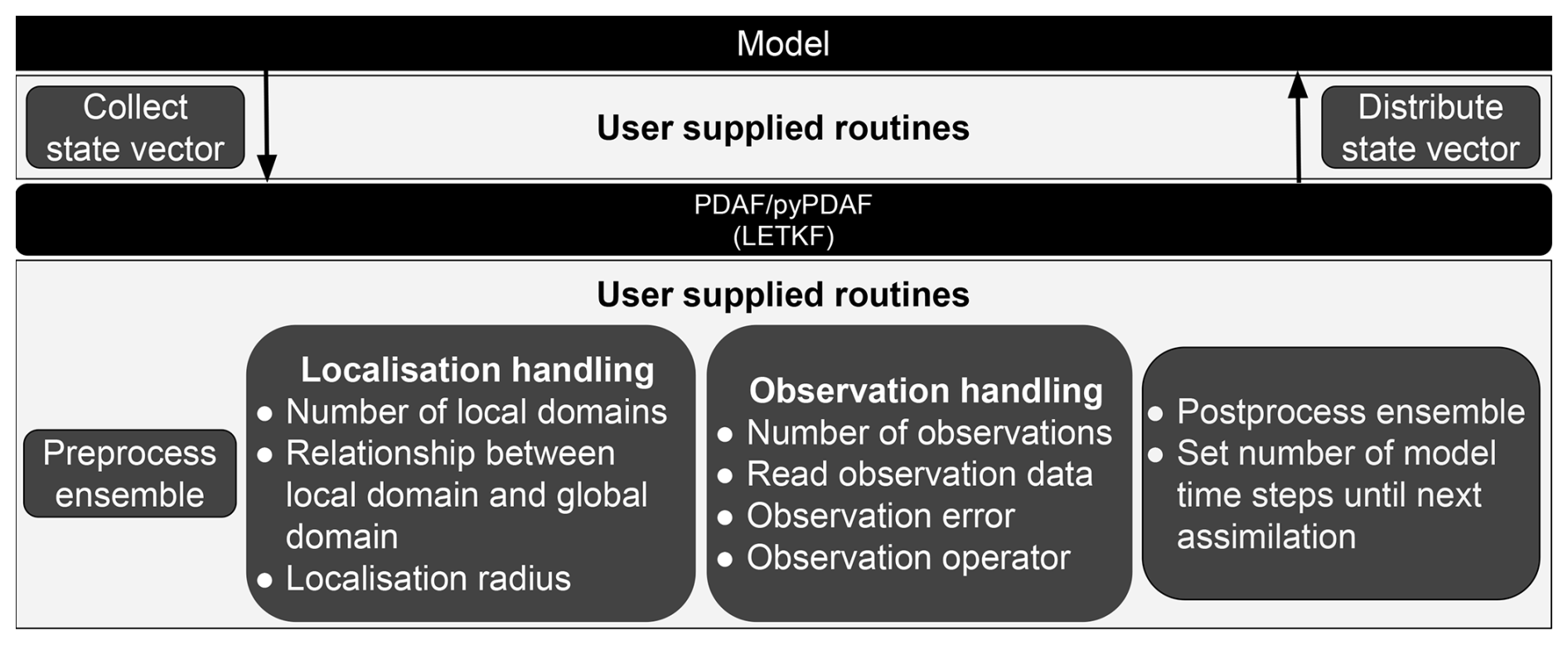
Figure 1 A schematic diagram of an online LETKF DA system using (py)PDAF. In the case of an offline DA system, the model can be its restart files.

To ensure that PDAF can be flexibly adapted to any models and observations, it requires users to provide case-specific information. This includes the information on the state vector, observations and localisation. The framework obtains this information via user-supplied functions which are external callback subroutines. Figure 1 shows a schematic diagram of an online DA system where the local ensemble transform Kalman filter (LETKF) is used. Here, the user-supplied functions connect PDAF with models. Called by the PDAF routines, these user-supplied functions collect state vectors from model forecasts and distribute the analysis back to the model for the following forecast phase. During the analysis step, user-supplied functions also pre- and post-process the ensemble, handle localisation and observations, and provide the number of model time steps for the following forecast phase. As the user-supplied functions depend on the chosen DA algorithm, other algorithms may require different functions. For example, a 3DVar DA system requires routines for the adjoint observation operator and control vector transformation. To ameliorate the difficulty in the observation handling, PDAF provides a scheme called observation module infrastructure (OMI). The OMI routines provide a structured way to handle the processing of observations and error covariance matrix used by DA algorithms, and provide support for the complex distance computation used by localisation. In the current version of PDAF V2.3, it also supports spatial interpolations on structured and unstructured grids for observation operators as well as an observation operator for observations located on grid points. The OMI also supports both diagonal and non-diagonal observation error covariance matrices. One can also implement PDAF without OMI, but additional functions would be required.

In an online DA system, the collection and distribution of state vector is an in-memory data exchange handled efficiently by PDAF. It is possible to implement an offline DA system with PDAF where the model in Fig. 1 is replaced by model restart files while the user-supplied collection and distribution routines manage the I/O operations of these restart files. Offline DA implementation is a crucially supported feature of PDAF and a potentially important use-case for pyPDAF, but we will not discuss it in detail for the sake of brevity. We will provide details of the implementation of user-supplied functions in the context of pyPDAF in Sect. 2.4.

2.2 Data assimilation methods in PDAF

PDAF supports a variety of DA methods with a focus on ensemble-based DA methods. Ensemble-based DA is a class of DA approaches that approximate the statistics of the model state and its uncertainty using an ensemble of model realisations. These DA methods are based on Bayes theorem where the prior, typically a model forecast, and posterior (analysis) distributions can be approximated by a Monte Carlo approach. The ensemble forecast allows for an embarrassingly parallel implementation which means that, with sufficient computational resources, the wall clock computational time of the forecast does not increase with the ensemble size.

The majority of ensemble DA methods are constructed under the Gaussian assumption of the forecast and analysis distributions such as the stochastic ensemble Kalman filter (EnKF, Evensen, 1994). The EnKF approximates the forecast and analysis error distribution by an ensemble. PDAF provides implementations for the EnKF and several of its variants. These variants improve the efficiency and reliability of the EnKF including singular evolutive intepolated Kalman filter (SEIK, Pham, 2001), ensemble transform Kalman filter (ETKF, Bishop et al., 2001), error space transform Kalman filter (ESTKF, Nerger et al., 2012). Other typical filtering algorithms, such as ensemble adjustment Kalman filter (EAKF, Anderson, 2001) and ensemble square root filters (EnSRF, Whitaker and Hamill, 2002), are not implemented in PDAF V2.3 used in this work but were introduced in the newer release V3.0. In practice, computational resources limit the feasible ensemble size in the high-dimensional realistic DA applications in the Earth system due to the cost of model forecasts. The ensemble-based DA approaches typically suffer from sampling errors from limited ensemble size. To mitigate these deficiencies, PDAF also provides common techniques such as covariance matrix inflation and localisation (e.g., Pham et al., 1998; Hamill et al., 2001; Hunt et al., 2007). In addition to EnKFs, PDAF also provides 3-dimensional variational methods. This includes variants of 3DEnVar (see  Bannister, 2017) that can be used to achieve flow-dependent background error covariance matrix, and/or to avoid explicit computation of the adjoint model in the minimisation process by using an ensemble approximation.

In addition, PDAF provides DA methods that can treat fully non-linear and non-Gaussian problems. This includes particle filters (see van Leeuwen et al., 2019). However, for high-dimensional geoscience applications, the classical particle filters suffer from the “curse of dimensionality” where the required ensemble size grows exponentially with the dimension of the state vector making the approach computationally infeasible. Therefore, PDAF also provides other non-linear filters such as nonlinear ensemble transform filter (NETF) and local Kalman–nonlinear ensemble transform filter (LKNETF, Tödter and Ahrens, 2015; Nerger, 2022). These methods mitigate the cost of nonlinear filters by restricting to the second-order moment of the statistical distribution.

2.3 pyPDAF

Depending on the users' programming skills, implementation of user-supplied functions can be laborious in Fortran and typical code development in Python can be less time consuming. Thanks to the integrated package management, code development in Python can rely on well optimised packages without the need for compilation. For these reasons, a variety of numerical models are implemented in Python (e.g., De Cruz et al., 2016; Abernathey et al., 2022; McGibbon et al., 2021; Bi et al., 2023). Hence, a Python interface to PDAF allows the design of an online DA system with such Python-based models. These range from low-dimensional toy dynamical systems to high-dimensional weather and climate systems. Compared to a Fortran-coded DA system, a Python DA system can be implemented efficiently with the aid of various external packages and allows for easier modifications without recompilation such that users can focus on scientific problems.

The pyPDAF package can also be applied to offline DA systems, i.e. coupling the model and data assimilation program through restart files. In an offline DA system, pyPDAF can be used without the restriction of the programming language of the numerical model. When computationally intensive user-supplied functions are well optimised, e.g., using just-in-time (JIT) compilation, this could also be used for high-dimensional complex models. Thus, depending on the requirements of the users, pyPDAF can also be used to prototype a Fortran DA system. The application of pyPDAF in high-dimensional models can also be enabled by its support of the parallel features of PDAF, which use the Message Passing Interface (MPI, Message Passing Interface Forum, 2023). For this, a pyPDAF DA system relies on the “mpi4py” package for MPI support. The pyPDAF system can also support shared memory parallelisation for DA algorithms using domain localisation in PDAF when built with OpenMP. However, the efficiency of OpenMP is restricted by the global interpreter lock in Python.

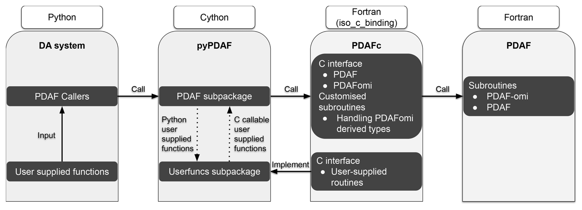
Figure 2 An illustration of the design of the pyPDAF interface to the Fortran-based framework PDAF. Here, only the Python component is exposed to pyPDAF users, and the Cython and Fortran implementations are internal implementations of pyPDAF.

As the reference implementation of Python is based on the C programming language (Python Software Foundation, 2024), the design of pyPDAF is based on the interoperability between the programming languages of C and Fortran using the iso_c_binding module of Fortran. As shown in Fig. 2, a C interface of PDAF, PDAFc, is developed in pyPDAF, which includes essential PDAF interfaces and interfaces for user-supplied functions. Due to this design, PDAFc could be used as an independent C library for PDAF. The pyPDAF implementation relies on the C-extension for Python (Cython). In Cython, Python datatypes are converted into C pointers to allow for information exchange between PDAF and pyPDAF. In pyPDAF, C callable functions are implemented to call user-supplied functions written in Python such that PDAF can utilise these user-supplied functions. The PDAF functionalities are provided through functions implemented in Cython, which are accessible from Python.

The pyPDAF design means that a DA system can be coded purely in Python utilising PDAF functions. The simplicity of a pure Python DA system depends on mixed programming languages and external libraries. The pyPDAF package itself is a mixed program of C, Fortran and Python. Moreover, as DA algorithms require high-dimensional matrix multiplications, PDAF relies on the numerical libraries LAPACK (linear algebra package) and BLAS (basic linear algebra subprograms). The mixed languages and libraries lead to a complex compilation process especially when users could use different operating systems. To fully utilise the cross-platform support of Python environment, pyPDAF is distributed via the package manager conda to provide an out-of-box user experience with pyPDAF where users can use pyPDAF without the need for compiling the package from the source code. Detailed installation instructions can be found at: Installation – pyPDAF documentation (2025).

pyPDAF allows for the use of efficient implementations of DA algorithms in PDAF. However, a DA system purely based on pyPDAF could still be less efficient than a DA system purely based on PDAF coded in Fortran. The loss of efficiency is partly due to the operations in user-supplied Python functions and the overhead from the conversion of data types between Fortran and Python. We will evaluate the implications of these loss of efficiency in Sect. 4.2.

2.4 Construction of data assimilation systems using pyPDAF

To illustrate the application of pyPDAF to an existing numerical model, as an example, we present key implementation details of an LETKF DA system. This example follows the schematic diagram in Fig. 1. Here, we assume that the number of available processors is equal to the ensemble size. Under this assumption, each ensemble member of the model forecast runs on one processor, and the analysis is performed serially on a single processor. We further assume that observations are co-located on the model grid but are of lower resolution, and they have a diagonal error covariance matrix.

A pyPDAF DA system can be divided into three components: initialisation, assimilation and finialisation. In this section, to associate the description with actual variable names in pyPDAF, the variable names in pyPDAF are given in brackets. In this system, the pyPDAF functionalities are initialised by a single function call

$$\begin{array}{rl}& \mathtt{\text{param\_int, param\_real, flag =}}\\ & \mathtt{\text{pyPDAF.PDAF.init(filtertype, subtype,}}\\ & \mathtt{\text{stepnull, param\_int, param\_real,}}\\ & \mathtt{\text{COMM\_model, COMM\_filter, COMM\_couple,}}\\ & \mathtt{\text{task\_id, n\_modeltasks, filterpe,}}\\ & \mathtt{\text{init\_ens\_pdaf)}}.\end{array}$$

In the initialisation step, the following information is provided to pyPDAF:

1. pyPDAF takes information on the type of filters (filtertype and subtype).

2. Corresponding to the filter type, the initialisation step also requires the size of the state vector and the ensemble size (dim_p and dim_ens in param_int respectively), and the inflation factor (param_real). These parameters allow PDAF to allocate internal arrays such as the ensemble mean (state_p) and the ensemble matrix (ens_p) used by the DA.

3. In addition to the filter configurations, the initialisation step also initialises the parallelisation used in PDAF, which requires the MPI communicators. These MPI communicators instruct PDAF on the functionalities of each processor and their communication patterns. Processors within the same model communicator (COMM_model) are used to perform the same ensemble member of model forecast. The number of model communicators is the same as the number of ensemble members run simultaneously (n_modeltasks). Each processor is associated with a specific ensemble member or model task by an index (task_id). During the DA step, PDAF will collect an ensemble matrix from the state vector residing in each model communicator via the coupling communicator (COMM_couple). The DA is performed on filter processors (filterpe = .true.) in one of the filter communicators (COMM_filter). Even though the parallelisation strategy can be freely designed by users, example parallelisation modules are readily available in pyPDAF. Detailed explanations of the parallelisation strategy used by PDAF can be found in Nerger and Hiller (2013a).

4. The initialisation step also prepares the system for future forecast-analysis cycling. Here, it takes the initial time step (stepnull) for step counters in PDAF.

5. In the initialisation step, the ensemble has to be initialised. In pyPDAF, this is achieved by the return values of a user-supplied function (state_p, uinv, ens_p, flag = init_ens_pdaf(filtertype, dim_p, dim_ens, state_p, uinv, ens_p, flag)). In this function, users have the flexibility to choose the initial ensemble. One can read an ensemble from files, or sample an ensemble from a covariance matrix. These can be assisted by input from PDAF via arguments of user-supplied functions. For example, PDAF provides the functionality of generating ensemble from singular vectors and values (uinv) of a covariance matrix using second-order exact sampling (Pham, 2001).

6. If OMI is used, the initialisation step also involves an additional function call (pyPDAF.PDAF.omi_init(n_obs)) to inform PDAF the number of observation types (n_obs) in the system.

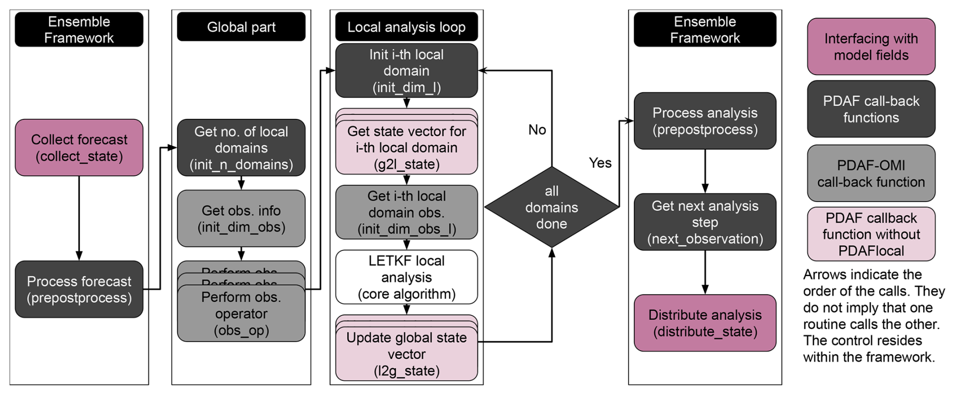
Figure 3 A flowchart of the sequence of LETKF operations in PDAF. These operations include user-supplied functions and core LETKF algorithm. The arrows indicate the order in which the user-supplied functions are executed. They do not imply that one routine calls the other. The observation operators and the global and local domain update are represented by multiple boxes as they are performed by each ensemble member.

In each model integration step, the function

$$\begin{array}{rl}& \mathtt{\text{status =}}\\ & \mathtt{\text{pyPDAF.PDAF.omi\_assimilate\_local}}\\ & \mathtt{\text{(collect\_state, distribute\_state,}}\\ & \mathtt{\text{init\_dim\_obs, obs\_op,}}\\ & \mathtt{\text{prepostprocess, init\_n\_domains,}}\\ & \mathtt{\text{init\_dim\_l, init\_dim\_obs\_l,}}\\ & \mathtt{\text{g2l\_state, l2g\_state, next\_observation)}}\end{array}$$

is called where all arguments specify the names of user-supplied functions handling operations specific to the model and observations. If the forecast phase is complete, the analysis step is executed. In the analysis step, each user-supplied function will next be executed by PDAF to collect necessary information, or perform case-specific operations for the DA. A flow chart is given in Fig. 3.

As shown in Fig. 1, the model and PDAF exchange information by user-supplied functions. First, a user-supplied function (state_p = collect_state(dim_p, state_p)) is executed by PDAF for each ensemble member to collect a state vector (state_p) from model forecast fields. Further, one has to provide a user-supplied function (state_p = distribute_state(dim_p, state_p)) such that, after the analysis step, the analysed state vector can be distributed back to model fields for the initialisation of the next forecast cycle. These user-supplied functions allow users to adapt a DA system with different models. For example, as mentioned in Sect. 2.2, optimal state estimation is achieved by ensemble-based Kalman filters under a Gaussian assumption. The state vector collection and distribution function can be used to perform Gaussian anamorphosis where non-Gaussian variables can be transformed to Gaussian variables (Simon and Bertino, 2012).

To handle different observations, with the OMI functionality, only three user-supplied functions need to be implemented:

Func 1:

a function that provides observation information like observation values, errors and coordinates (dim_obs = init_dim_obs(step, dim_obs)) where its primarily purpose is to provide the dimension of observation vector (dim_obs) to PDAF,

Func 2:

a function that provides the observation operator (m_state_p = obs_op(step, dim_p, dim_obs, state_p, m_state_p)), where the observation operator transforms the state vector (state_p) into observation space (m_state_p),

Func 3:

a function that specifies the number of observations being assimilated in each local domain (dim_obs_l = init_dim_obs_l (domain_p, step, dim_obs, dim_obs_l)).

In Func 1, the dimension of the observation vector for the i_obs-th observation type can be calculated by PDAF function (dim_obs = pyPDAF.PDAF.omi_gather_obs(i_obs, obs_p, ivar_obs_p, ocoord_p, cradius)) directly by providing observation vector (obs_p), inverse of the observation error variance (ivar_obs_p), the spatial coordinates of observations (ocoord_p), and a cut-off localisation radius (cradius). In this user-supplied function, one also sets additional observation attributes (obs_f) including the switch for assimilating the observation type (doassim), the indices of the observations in the state vector (id_obs_p), the domain size and the options for distance computation in localisation. These attributes can be set by setter functions (e.g., pyPDAF.PDAF.omi_set_id_obs_p(i_obs, id_obs_p)).

In Func 2, similar to functions used in Func 1, observation operators that transform a model field to observations located on grid points (m_state_p = pyPDAF.PDAF.omi_obs_op_gridpoint(i_obs, state_p, m_state_p)) are provided by PDAF. One can construct more complex observation operators in pyPDAF (e.g., Shao and Nerger, 2024), but is not discussed here for the sake of simplicity. The goal of Func 3 can be achieved by an OMI function (dim_obs_l = pyPDAF.PDAF.omi_init_dim_obs_l_iso(i_obs, coords_l, locweight, cradius, sradius, dim_obs_l)). The OMI function automatically handles observations and their error variances used in the local domain given the coordinates of a local domain (coords_l), the type of localisation weight (locweight), and the cut-off localisation radius (cradius) as well as the support radius of specified localisation function (sradius).

Users must specify information for domain localisation in four additional user-supplied functions. These include the number of local domains (n_domains_p = init_n_domains(step, n_domains_p)), the dimension of the state vector in the domain_p-th local domain (dim_l= init_dim_l(step, domain_p, dim_l)), the conversion of the full global state vector to a state vector on a local domain (state_l = g2l_state(step, domain_p, dim_p, state_p, dim_l, state_l)) and vice versa (state_p = l2g_state(step, domain_p, dim_l, state_l, dim_p, state_p)). The user-supplied function g2l_state and l2g_state are not used in “PDAFlocal” modules as will be discussed in Sect. 4.2.

In addition to information on the state vector, observations and localisation, the pre- and post-processing of the ensemble is also case-specific. Therefore, this operation must also be performed by a user-supplied function (state_p, uinv, ens_p = prepostprocess(step, dim_p, dim_ens, dim_ens_p, dim_obs_p, state_p, uinv, ens_p, flag)). This function allows the user to perform arbitrary operations on the ensemble directly before (pre-processing) or after (post-processing) the analysis step update.

One last piece of case-specific information is the control of DA cycles. In the user-supplied function (nsteps, doexit, time = next_observation(step, nsteps, doexit, time)), users specify the number of time steps (nsteps) until the next analysis step is computed (thus the duration of the forecast phase). Given the current time step, PDAF also obtains the information of the current model time (time) and a flag for the completion of all DA cycles (doexit).

In the completion of the DA system, to control the memory allocation in the DA process, the DA system should be finalised by a clean-up function (pyPDAF.PDAF.deallocate()).

PDAF can handle much more complex cases including non-isotropic localisation, or non-diagonal observation error covariance matrices. Besides LETKF, other filters might require different user-supplied functions as they utilise different case-specific information. The provided pyPDAF example code that exists can support a wide range of filters without changes.

3 Application example

To demonstrate the application of pyPDAF and to evaluate its performance in comparison to PDAF, we set up coupled DA experiments with MAOOAM (De Cruz et al., 2016) version 1.4. The original MAOOAM model is written in Fortran that is implemented directly with PDAF, and a wrapper for Python is developed in this study such that MAOOAM can be coupled with pyPDAF. This means that two online DA systems using Fortran and Python are developed respectively to allow for a comparison between the PDAF and pyPDAF implementation. In these DA systems, a suite of twin experiments is carried out using the ensemble transform Kalman filter (ETKF, Bishop et al., 2001) and its domain localisation variant, LETKF.

3.1 MAOOAM configuration

The MAOOAM solves a reduced-order non-dimensionalised quasi-geostrophic (QG) equation (De Cruz et al., 2016). Using the beta-plane approximation, the model has a two-layer QG atmosphere component and one-layer QG shallow-water ocean component with both thermal and mechanical coupling. For the atmosphere, the model domain is zonally periodic, and has a no-flux boundary condition meridionally. For the ocean, no-flux boundary conditions are applied in both directions. This setup represents a channel in the atmosphere and a basin in the ocean. The model variables for the two-layer atmosphere are averaged into one layer. Accordingly, MAOOAM consists of four model variables: the atmospheric streamfunction, ψ_a, the atmospheric temperature, T_a, the ocean streamfunction, ψ_o, and the ocean temperature, T_o. The model variables are solved in spectral space. The spectral basis functions are orthonormal eigenfunctions of the Laplace operator subject to the boundary condition, and the number of spectral modes is characterised by harmonic wave numbers P, H, M (Cehelsky and Tung, 1987).

Our model configuration adopts the strongly coupled ocean and atmosphere configuration “36st” of Tondeur et al. (2020) using a time step of 0.1 time units corresponding to around 16 min. Using the notation of $H^{max}x-P^{max}y$ of De Cruz et al. (2016) with the superscript max the maximum number of harmonic wave numbers, the configuration chooses 2x−4y modes for the ocean component and 2x−2y modes for the atmosphere component. This leads to a total of 36 spectral coefficients with 10 modes for ψ_a and T_a respectively and 8 modes for ψ_o and T_o respectively. The model runs on a rectangular domain with a reference coordinate system of $(x\times y)\in [\mathrm{0},\frac{\mathrm{2}\mathit{\pi }}{n}]\times [\mathrm{0},\mathit{\pi }]$, where n=1.5 is the aspect ratio between the x and y dimensions.

In contrast to Tondeur et al. (2020) who assimilate in the spectral space, we assimilate in the physical space in which real observations are usually available. Assimilating in the physical space is not only more realistic but also provides the possibility to investigate the computational efficiency of pyPDAF without changing the model dynamics. This is because the same number of spectral modes can be transformed to different number of grid points. This allows us to focus on the computational cost of the DA. Therefore, for benchmarking computational cost, we conduct a suite of SCDA experiments with ${\mathrm{2}}^k+\mathrm{1}\times {\mathrm{2}}^k+\mathrm{1}$ grid points where $\mathrm{7}\le k\le \mathrm{11}$. This gives us state vectors with dimensions ranging from a magnitude of 10⁴ to 10⁷. We also implement SCDA experiments using LETKF on a grid number size of 257×257 with observations on every 4 and 8 grid points to investigate the efficiency of the domain localisation in pyPDAF.

We integrate MAOOAM with (py)PDAF. As shown in Fig. 1, the key ingredient of coupling MAOOAM with (py)PDAF is the collection and distribution of state vectors. In the user-supplied function that collects the state vector for pyPDAF (see Fig. 1), spectral modes of the model are transformed from the spectral space to physical space using the transformation equation,

$$\begin{array}{}\text{(1)}& f(x,y,t)=\sum _{i=\mathrm{1}}^K{c}_i\left(t\right)F_i(x,y),\end{array}$$

where $f(x,y,t)$ is any model variable in the physical space, K is the number of modes, c_i(t) is the spectral coefficient of the model variable, F_i(x,y) is the spectral basis function of mode i outlined in De Cruz et al. (2016). In the user-supplied function that distributes the state vector for pyPDAF (see Fig. 1), the analysis has to be transformed back to the spectral space to initialise the following model forecast. The inverse transformation from the physical space to the spectral space can be obtained by

$$\begin{array}{}\text{(2)}& c_i\left(t\right)={\displaystyle \frac{n}{\mathrm{2}{\mathit{\pi }}^{\mathrm{2}}}}\underset{\mathrm{0}}{\overset{\mathit{\pi }}{\int }}\underset{\mathrm{0}}{\overset{\frac{\mathrm{2}\mathit{\pi }}{n}}{\int }}f(x,y,t)F_i(x,y)\mathrm{d}x\mathrm{d}y.\end{array}$$

where n is the ratio between meridional and zonal extents of the model domain. Here, each basis function corresponds to a spectral coefficient of the model variable. The basis functions are evaluated on an equidistant model grid. The spectral coefficients are obtained via the Romberg numerical integration. The accuracy of the numerical integration depends on the spatial resolution and the number of grid points with an error of $\mathcal{O}\left(n^{-\mathrm{2}{\log }_{\mathrm{2}}n}\right)$ where n is the number of grid points. Our experiments suggest that the numerical integration error is negligible once we have $({\mathrm{2}}^{\mathrm{7}}+\mathrm{1}\times {\mathrm{2}}^{\mathrm{7}}+\mathrm{1})$ = (129×129) grid points. In this study, for the sake of efficiency, the transformation between spectral modes and grid points are implemented in Fortran. In pyPDAF systems, the Fortran transformation routines are used by Python with “f2py”. This implementation ensures that the numerical computations do not render rounding errors when conducted in different programming languages. Moreover, it also demonstrates that the computationally intensive component of user-supplied functions can be sped up by optimised Fortran code.

3.2 Experiment design

In a twin experiment, a long model run is considered to represent the truth. The model state is simulated with an initial condition sampled in the spectral space following a Gaussian distribution, 𝒩(0,0.01). The DA experiments are started after 9×10⁵ time steps corresponding to around 277 years of model integration to ensure that the initial state corrected by the DA follows the trajectory of the dynamical model.

The observations are generated from the truth of the model state based on pre-defined error statistics of the observations. Except for the LETKF experiments, both atmosphere and ocean observations are sampled every 8 model grid points for each model grid setup. In all cases, the observation error standard deviations are set to 50 % and 70 % of the temporal standard deviation of the true model trajectory at each grid point for the atmosphere and ocean respectively. This leads to spatially varying observation errors with regions of larger or smaller observation errors. The atmospheric processes in MAOOAM show variability on shorter timescales than the ocean. Hence, the ocean observations are assimilated around every 7 d (630 time steps) while the atmosphere observations are assimilated around every day (90 time steps). This is in line with the experiment setup in Tondeur et al. (2020).

As shown by Tondeur et al. (2020), DA in the model configuration using 36 spectral coefficients can achieve sufficient accuracy with 15 ensemble members. In this study, 16 ensemble members are used, and each ensemble member runs serially with a single process. Without tuning, a forgetting factor of 0.8 is applied to maintain the ensemble spread. The forgetting factor (Pham et al., 1998) is an efficient approach to multiplicative ensemble inflation in which the covariance matrix is inflated by the inverse of the forgetting factor as shown in the formulation in Nerger et al. (2012).

PDAF provides functionality to generate the ensemble. Here, to demonstrate its functionality, we use second-order exact sampling (Pham, 2001), in which the ensemble is generated from a covariance matrix. The covariance matrix is estimated using model states sampled every 10 d over a 100-year period, based on the trajectory of the truth model after approximately 1000 years from the start of the simulation. This leads to a covariance matrix with 36 non-zero singular values equalling to the number of spectral modes in the model. The ensemble generated from the covariance matrix could violate the dynamical consistency of the model, so that the ensemble would need to be spun up to reach dynamical consistency. To reduce the spin up time, the initial perturbation is scaled down by a factor of 0.2, 0.15, 0.4 for Ψ_a, T_a and T_o respectively. Because the ocean streamfunction has very low variability, its perturbation is unchanged.

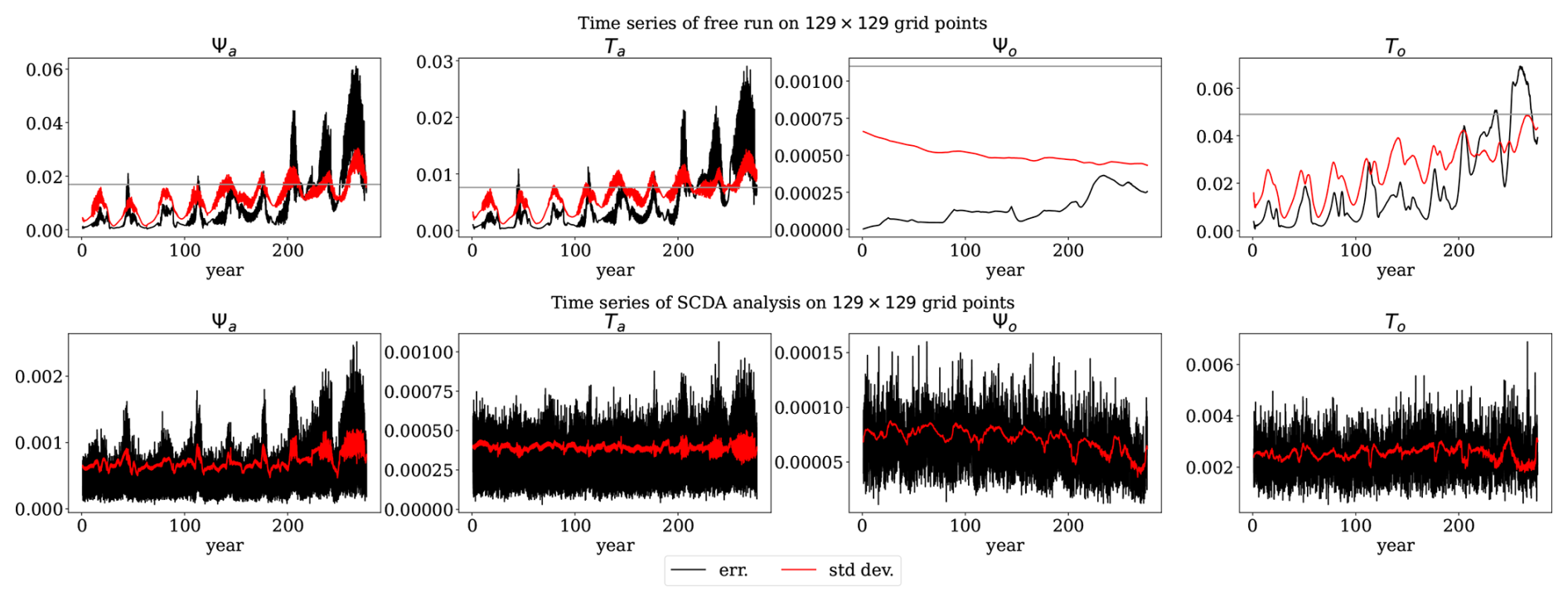
Figure 4 Ensemble standard deviation and RMSE of the (top) free run and (bottom) SCDA analysis on a 129×129 grid. Shown are the time series of the spatial mean of ensemble spread (red) and the RMSE of the analysis (black). The atmosphere shows fast variability and oscillatory RMSE of the ensemble mean while the RMSE of the ocean ensemble mean is smooth. The horizontal grey line is the spatial averaged observation error.

The DA experiments are started after 15 d from the beginning of the ensemble generation. The DA experiments are then run for another 9×10⁵ time steps which is around 277 years. In this setup, the forecast error is solely a result of inaccuracy of initial conditions. As shown in Fig. 4, the ensemble spread captures the trend, and has a similar magnitude as the model forecast error. This suggests that the forecast uncertainty of the free run ensemble is able to reflect the forecast errors even though the spread is lower than the RMSE after 200 years.

In the free run (upper panel of Fig. 4), the ocean streamfunction shows a very slow error growth rate. This is also shown by the ensemble uncertainty. Sensitivity tests (not shown) suggest that an increased RMSE of the ocean streamfunction has a strong impact on the model dynamics consistent with the theoretical discussion given in Tondeur et al. (2020). The RMSE of the atmosphere components shows a wave-like behaviour in time. Tondeur et al. (2020) describe the periods associated with fast dynamics with high and oscillatory RMSEs as active regimes and the periods associated with slow dynamics with low and stable RMSEs as passive regimes.

As a case study to demonstrate the capability of pyPDAF, both SCDA and WCDA are implemented. In WCDA, each model component performs DA independently even though the forecast is obtained by the coupled model. This means that the observations only influence their own model component in the analysis step which implies two separate DA systems. In an online DA setup in PDAF, two separate state vectors have to be defined in each analysis step which is not straightforward with PDAF due to its assumption that each analysis step has only one state vector. In the case of AWI-CM in Tang et al. (2021), two separate state vectors were obtained by using parallelisation, but here the two model components of MAOOAM are run using the same processor. In our implementation we obtain WCDA by resetting the time step counter in PDAF such that even if the assimilation of two state vectors are done by using PDAF twice, PDAF only counts it as one analysis time step. An alternative approach could be to use the LETKF method, and define the local state vector as either the atmosphere or ocean variables.

Compared to the WCDA, atmosphere observations influence the ocean part of the state vector and vice versa in the SCDA. This means that the coupling occurs for both the analysis step and model forecast. In this case, the DA system only has one unified state vector that contains the streamfunction and temperature of both model components. The implementation of an online SCDA system aligns with the design of PDAF, and does not require special treatment.

3.3 Comparison of pyPDAF and PDAF implementation of CDA

As pyPDAF is an interface to PDAF, the same number of user-supplied functions are used for DA systems implemented with pyPDAF and PDAF. As detailed in Sect. 2.4, the ETKF system requires 7 user-supplied functions. For the LETKF system, an additional 5 user-supplied functions are needed. However, as will be discussed in Sect. 4.2, if “PDAFlocal” modules are used, the additional user-supplied function necessary for domain localisation can be reduced to 3.

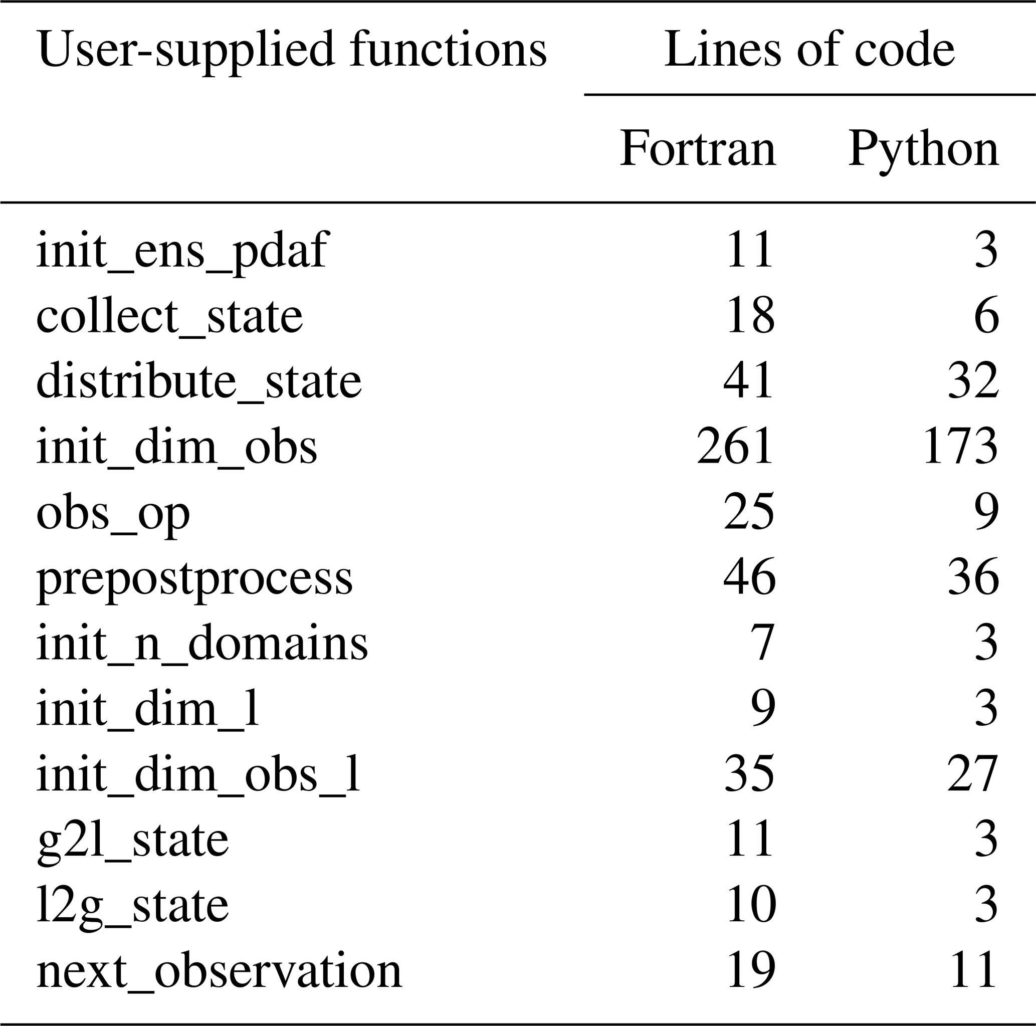
One of the major advantages of pyPDAF is the ease of implementation. Here, to partially reflect the difference in implementation difficulty between pyPDAF and PDAF, the number of lines of code between pyPDAF and PDAF in each user-supplied functions is compared in Table 1. We recognise that such comparison can be inaccurate due to different coding styles and potential unaccounted boilerplate code. Moreover, fewer lines of code do not necessarily represent improved ease of implementation as the DA system setup typically involves scientific research besides code implementation. Nevertheless, we show that Python implementation needs fewer lines of code than Fortran implementation for all user-supplied functions. The reduced implementation difficulty can be attributed to: (1) the Python implementation can make use of efficient third-party Python packages utilising vectorisation avoiding loops and manual implementation; (2) the Python programming language does not require static typing which is required by Fortran; (3) the Python programming language allows for extensible and flexible implementation due to its language features.

Table 1 Number of lines of code broken down by user-supplied functions between Fortran and Python implementation of a strongly coupled DA system. The count removes comments and empty blank lines. In the “init_dim_obs” function, we count the total lines of code including functions called within the user-supplied functions and boilerplate code for class definition. The “prepostprocess” is divided into three functions in Python where we count the total lines of code here.

4 Results

In this section, to validate the MAOOAM-(py)PDAF online DA system, we evaluate its DA skill. For the sake of efficiency, the skill of DA is assessed on a domain with 129×129 grid points. To evaluate the computational efficiency of pyPDAF and PDAF and the potential practical applications of pyPDAF, we compare the wallclock time in the SCDA system.

The online DA systems using PDAF and pyPDAF produce quantitatively the same results in all experiments up to machine precision. This is because the user-supplied functions mainly perform file handling and variable assignments, but no numerical computations. An exception is only the spectral transformation described in Sect. 3.1. To ensure comparable numerical outcome, the numerical computations that affect the forecast and analysis, in particular the spectral transformation, are all conducted in Fortran in this work. These Fortran implementations are used by Python user-supplied functions using “f2py”. Note that, when numerical computations involve different programming languages, the model trajectory of the nonlinear system could differ because of errors in the initial conditions arising from rounding errors.

4.1 Skill of data assimilation

The time averaged RMSE of WCDA is smaller than that of the unconstrained free run as shown by Fig. 5. Thus, the error growth is successfully controlled by DA. This also demonstrates that the ETKF leads to a converged analysis even though our observations are less accurate than the forecast at the start of the DA period. The results also show that sparse observations can successfully control errors in regions without observations. This is due to the fact that the model fields are rather smooth leading to long ensemble correlations.

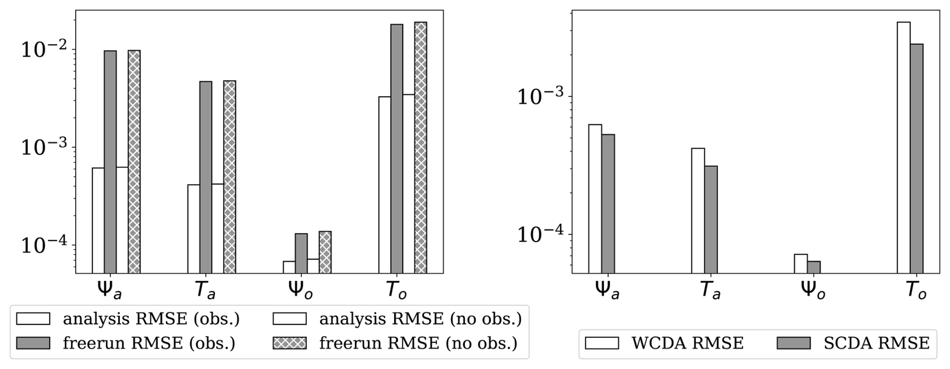
Figure 5 Left: The time-averaged RMSE of the analysis using WCDA and free run where the RMSE of the observed (non-hatched bars), denoted by “obs.” in the legend, and unobserved gridpoints (hatched bars), denoted by “no obs.”, are compared separately. Right: comparison of RMSEs for weakly and strongly coupled DA for all grid points. The y-axis is plotted in the log-scale.

As expected, the SCDA yields lower analysis RMSEs than the free run as shown in Fig. 4, and the RMSEs are also lower than the WCDA as shown in the right panel of Fig. 5. The improved analysis in the SCDA in each model component is a result of assimilating observations from the other model component. The effective use of these additional observations relies on the error cross-covariance matrix between model components estimated by the forecast ensemble. The improvements suggest a reliable error cross-covariance matrix in the coupled DA system.

These results suggest that both pyPDAF and PDAF can be used to implement a DA system as expected.

4.2 Computational performance of PDAF and pyPDAF

One motivation of developing a Python interface to PDAF is that the efficient DA algorithms in PDAF can be used by pyPDAF while the user-supplied functions can be developed with Python. However, the user-supplied functions provided by Python are expected to be slower than a pure Fortran implementation. The slow-down is both a result of lack of compilation in Python and the type cast between Fortran arrays and Python objects. Here we present a comparison of the wall clock time of both PDAF and pyPDAF experiments with standard SCDA broken down to the level of subroutines. Each experiment runs 100 analysis steps, and each experiment is repeated 10 times. The computation runs on the computing facility of University of Reading on a node with two AMD EPYC 7513 32-Core processors which have a 2.6 GHz frequency. With 16 ensemble members, each member uses a single processor for model forecast, and the DA is performed serially on a single processor.

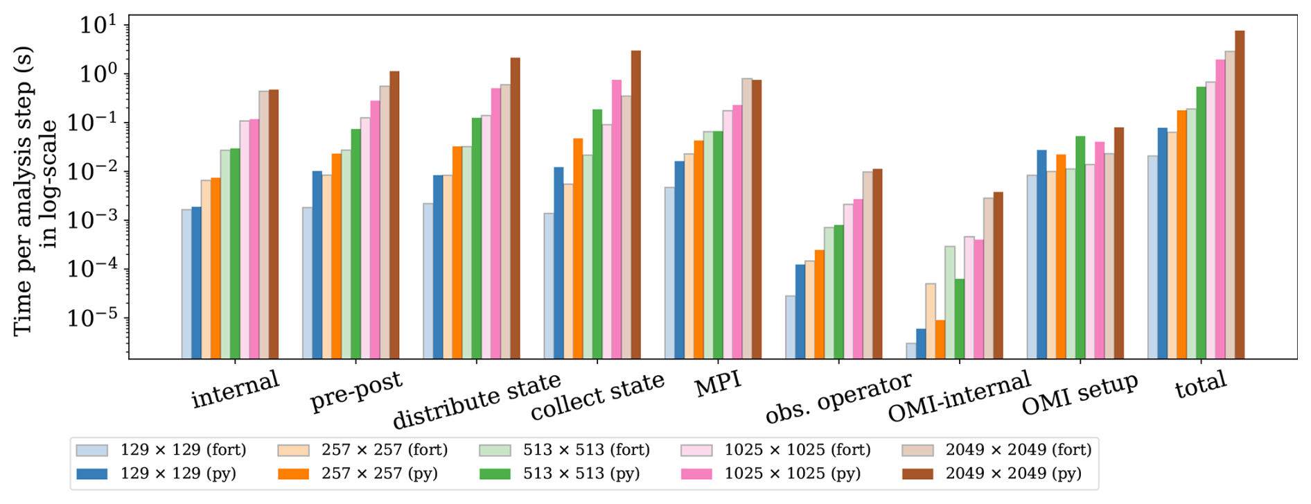
Figure 6 Wall clock time of pyPDAF (dark colour bars) and PDAF (light colour bars) systems per analysis step broken down by functionalities in SCDA ETKF experiments and their total wallclock time per analysis step in log-scale.

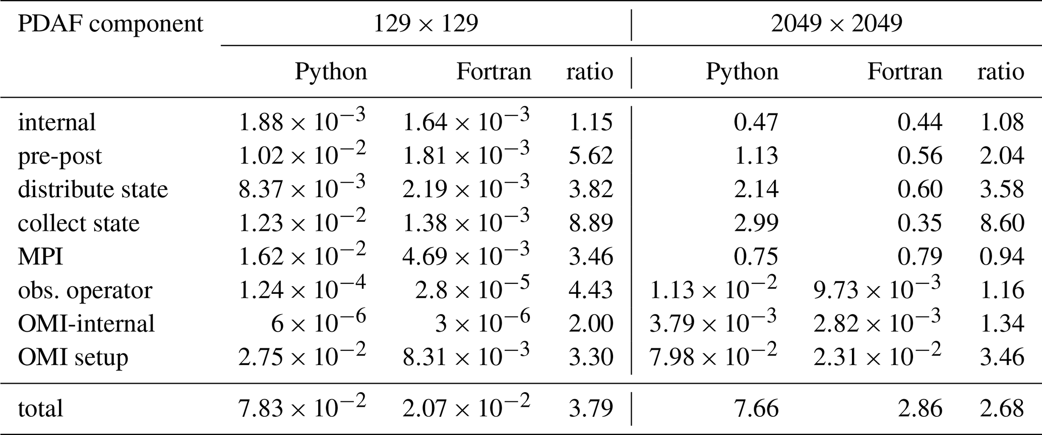
Table 2 Wall clock time per analysis step of pyPDAF and PDAF for each component of SCDA ETKF using 129×129 grid points and 2049×2049 grid points in seconds. The table also shows the ratio of the wall clock time between Python and Fortran. The wall clock time is the same as the wall clock time shown in Fig. 6.

The serial DA execution is primarily due to the default parallelisation strategy in PDAF. The ETKF has a straightforward parallelisation since the global transform matrix can be computed in a distributed form followed by a global sum. The LETKF is embarrassingly parallel for each local domain after communicating the necessary observations. Each processor can perform LETKF independently for their local domains. In PDAF, the parallelisation of both ETKF and LETKF is implemented in combination with domain decomposition of the numerical model. In this study, no domain decomposition is carried out for the numerical model itself. Thus, all local domains are located in one single processor for LETKF. The parallelisation strategy of PDAF is further explained in Nerger et al. (2005) and a pyPDAF documentation is available (Chen, 2025c).

As shown in Fig. 6 and Table 2, the PDAF-internal procedures (labelled “internal”), which are the core DA algorithm, take nearly the same amount of time per analysis step for PDAF and pyPDAF regardless of the number of grid points. As expected, the user-supplied functions take more computational time in the DA system based on pyPDAF than PDAF. In this study, the pre- and post-processing of the state vector (labelled “pre-post”) calculates the square root of the spatial mean of ensemble variance. The pre- and post-processing is implemented as a user-supplied function (see Sect. 2.4) which is computationally intensive. The intensive computations suit well for the use of the Python JIT compilation. The computational time of the pre- and post-processing increases with the size of the state vector, and Python is in general slower than the Fortran implementation. The difference of wall clock time between the pyPDAF and PDAF-based DA system decreases with increasing state vector size as the overhead in pyPDAF takes smaller portion of the total computation time compared to the floating-point computations. As a comparison shown in Table 2, the ratio of total computational time per analysis step for “pre-post” procedures between pyPDAF and PDAF implementation reduces to 2.04 on a 2049×2049 grid from 5.62 on a 129×129 grid. The overhead in the pyPDAF system is less affected by the dimension of the state vector for the distribution and collection of state vector (labelled “distribute state” and “collect state”) because these functions only exchange information between model and PDAF without intensive computation. For example, the pyPDAF system takes 3.82 and 8.89 times of computational time of the PDAF system for “distribute state” and “collect state” respectively on a 129×129 grid, which is similar to the ratio of 3.58 and 8.60 on a 2049×2049 grid. In addition to assigning a state vector to model fields and vice versa in Python, these user-supplied functions perform conversion between physical and spectral space based on Eqs. (1) and (2). As mentioned in Sect. 3.1, the transformation utilises the same Fortran subroutines for both PDAF and pyPDAF system which shows little contribution to the computational time between PDAF and pyPDAF. In the pyPDAF system, the Fortran subroutines are converted to Python functions by “f2py”. The computational time taken by these functions is proportional to the number of grid points. In this study, the MPI communications are only used to gather an ensemble matrix from the state vector of each ensemble member located at their specific processor. These communications, which are internal to PDAF and are not exposed to users, show little differences between pyPDAF and PDAF system.

The wall clock time used for handling observations shows that a pyPDAF DA system is in general slower than a PDAF system. With a low-dimensional state vector, the observation operator (labelled “obs. operator”) is slower in a pyPDAF system than PDAF even if the observation operator function only calls a PDAF subroutine provided by OMI. The slow-down of the pyPDAF system is again a result of overhead in the conversion of Fortran and Python arrays. Here, similar to the collection and distribution of the state vector, the function is called by each ensemble member. The overhead takes only a small fraction of the total computation time for high-dimensional state vectors, while the computing of the observation operator dominates the total computational time of the call. The internal operations of OMI (labelled “OMI internal”) are efficient and, in some cases, the pyPDAF systems can be more efficient than PDAF systems. Our experiments do not show clear benefits between pyPDAF and PDAF system for these operations, as expected especially considering the short wall clock time at an order of 10⁻⁶ with 129×129 grid points used in these operations. The setup of the OMI functionality is implemented in the user-supplied function of init_dim_obs (see Sect. 2.4). This includes reading and processing the observation data and their errors. In this case, the pyPDAF-based system is more expensive than the PDAF system. The pyPDAF system takes 3.30 (3.46) times of the computational time used to execute init_dim_obs in PDAF system on a 129×129 (2049×2049) grid. The relative increase of computational time between the pyPDAF and PDAF system is not evident even though a larger number of observations needs to be processed.

Our comparison shows that the interfacing between Python and Fortran yields overheads in the pyPDAF system even if we utilise JIT compilation of Python. Users need to consider a trade-off between these overheads and the ease of implementation in pyPDAF compared to PDAF. The differences of the computational cost can take a smaller portion of the total computation time for high-dimensional systems for the ETKF DA system without localisation due to increased numerical computations.

In practice, localisation is used to avoid sampling errors in high-dimensional weather and climate systems. To make full use of the computational resources, these high-dimensional systems are parallelised by domain decomposition. PDAF exploits the feature of these models for domain localisation where the state vector is also domain decomposed. Here, we choose a domain with 257×257 grid points to assess the LETKF with a cut-off localisation radius of 1 non-dimensionalised spatial unit. This corresponds to 3000 km covering around a third of the domain. As no domain decomposition is implemented for MAOOAM, each processor contains 257×257 local domains which is similar to the number of local domains used in a single processor of a domain decomposed global climate model.

For each local domain, the LETKF computes an analysis using observations with a localisation cut-off radius. Hence, the computational cost depends on the observation density. To investigate the effect of increased intensity of computations on the pyPDAF overhead, we add experiments that observe every 4 grid points.

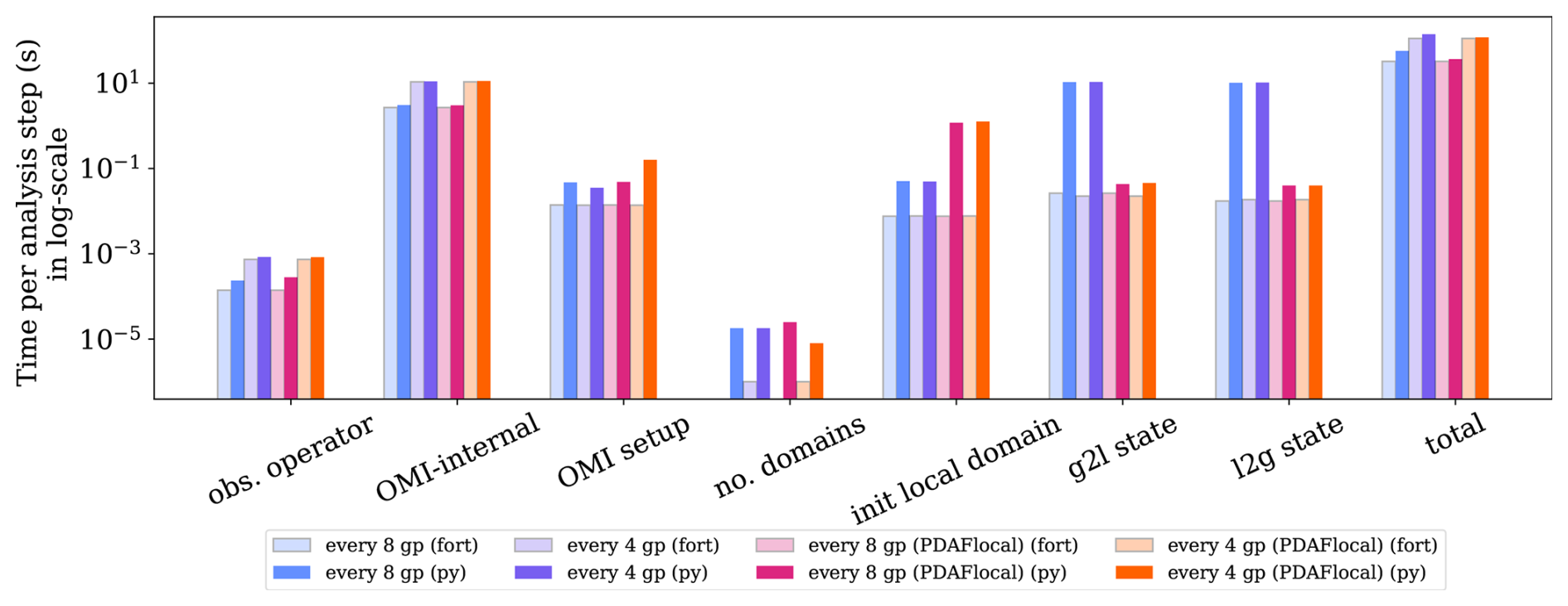
Figure 7 Wall clock time of pyPDAF (light colour bars) and PDAF (dark colour bars) system per analysis step broken down by functionalities in SCDA LETKF experiments and their total wallclock time per analysis step in log-scale with a 257×257 grid points. The left four bars (blue and purple bars) represent the case without using the PDAFlocal module while the rest uses the PDAFlocal module. For the sake of conciseness, the functionalities shared by both ETKF and LETKF are omitted. The computational time of PDAF system for “no. domains” is negligible when every 8 grid points are observed which lead to an empty bar.

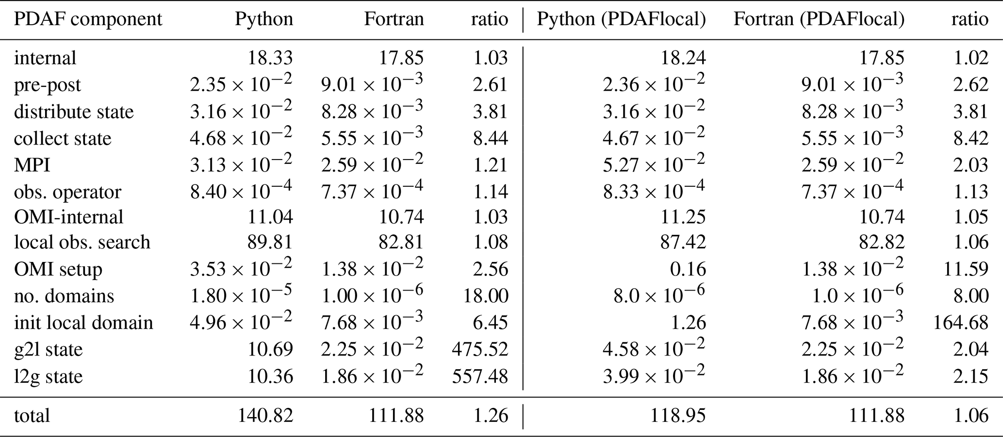
Table 3 Wall clock time per analysis step of pyPDAF and PDAF for each component of SCDA LETKF using 257×257 grid points in seconds where observations are taken every 4 grid points. The table also shows the ratio of the wall clock time between Python and Fortran. The wall clock time is the same as the wall clock time shown in Fig. 7.

As shown in Fig. 7, the increased observation density leads to an increase in computational time for the internal operations, observation operator, and the OMI-internal operations due to the larger number of locally assimilated observations. For example, for applying the observation operator, when every 8 grid points are observed, $\sim \mathrm{2.4}\times {\mathrm{10}}^{-\mathrm{4}}$ and $\sim \mathrm{1.4}\times {\mathrm{10}}^{-\mathrm{4}}$ s are respectively used in pyPDAF and PDAF systems, but in the case of observations for every 4 grid points, $\sim \mathrm{8.4}\times {\mathrm{10}}^{-\mathrm{4}}$ and $\sim \mathrm{7.4}\times {\mathrm{10}}^{-\mathrm{4}}$ s is used in pyPDAF and PDAF systems respectively. The increased observation density shows little influence on the computational cost of other user-supplied functions. For example, in the case of the OMI setup, when every 8 grid points are observed, ∼0.047 and ∼0.014 s is used in the pyPDAF and PDAF systems respectively, and in the case of observations for every 4 grid points, a similar computational time of ∼0.035 and ∼0.0137 s is used in pyPDAF and PDAF systems respectively. However, as the increased observation density leads to more intensive computations, this mitigates the gap of the total computational time between pyPDAF and PDAF system. In particular, as shown in Table 3 the run times for the internal operations of PDAF and OMI (“OMI-internal”) dominate the overall run time of the analysis step and show little difference for the pyPDAF and PDAF DA systems. The similar computational time applies for the case when PDAF searches for local observations for analysis local domains due to its intensive numerical computation. Here, when executing “OMI-internal” operations, when every 8 grid points are observed, ∼3.07 and ∼2.69 s is used in pyPDAF and PDAF systems respectively, but in the case of observations for every 4 grid points, ∼11.04 and ∼10.74 s is used in pyPDAF and PDAF systems respectively.

We notice large overhead in the pyPDAF system for user-supplied functions related to domain localisation. The “no. domains” user-supplied function takes $\sim \mathrm{1.8}\times {\mathrm{10}}^{-\mathrm{5}}$ s per analysis step for pyPDAF system but only $\sim \mathrm{1}\times {\mathrm{10}}^{-\mathrm{6}}$ s is taken by the PDAF system. The latter can be negligible when every 8 grid points are observed. In this user-supplied function, only one assignment is executed in the user-supplied function. Therefore, the overhead is primarily a result of conversion between the interoperation between Fortran and Python. This operation has little impact on the overall efficiency of the system. The computation takes 6.45 times of computational time of PDAF system in the pyPDAF system for the function specifying the dimension of the local state vector (“init local domain”) as shown in Table 3. The increased computational cost is a result of repeated execution of the user-supplied functions for each local domain. Specifically, in our experiment, this user-supplied function is used $\mathrm{257}\times \mathrm{257}\times \mathrm{4}$ times per analysis step. The overhead is even higher for the user-supplied functions that convert between local state vector and global state vector (“g2l state” and “l2g state” respectively), which are called for each ensemble member, due to the conversion of arrays instead of integers. In this experiment, the execution of these routines in pyPDAF can be even more than 500 times slower than in the PDAF system. As these operations are not computationally intensive, the overhead cannot be mitigated by JIT compilation. Without modifications in the PDAF workflow, the overhead can become comparatively smaller with high observation density arising from increased computational cost of other routines, or increased parallelisation of model domains leading to reduced number of local domains on each processor.

To overcome the specific run time issue of “g2l state” and “l2g state”, we developed a PDAFlocal module in PDAF, included in release version 2.3, where the user-supplied functions of “g2l state” and “l2g state” are circumvented in the PDAF interface as their operations are performed in the compiled Fortran code of PDAFlocal. This leads to similar computational cost of these functions in the pyPDAF and PDAF systems. With PDAFlocal, users need to implement an index vector providing the relationship between the state vector in the current local domain and the global state vector when local domain is initialised in “init local domain”. Due to this, with PDAFlocal, we see an increased computational time in “init local domain” in pyPDAF, which is around 160 times slower than the PDAF system. However, this pyPDAF overhead for “init local domain” is smaller than that of “g2l state” and “l2g state” due to the different types of operations and hence a lower number of array conversions between Fortran and Python in “init local domain”. Further, only one instead of three user-supplied functions are implemented in Python. With the enhancement by PDAFlocal, the total computing time is nearly equal for pyPDAF and PDAF with only 6 %–13 % higher time for pyPDAF.

Table 4 Wall clock time per analysis step of pyPDAF and PDAF for each component of SCDA ETKF in seconds with different ensemble members using 257×257 grid points where observations are taken every 8 grid points. The table also shows the ratio of the wall clock time between Python and Fortran.

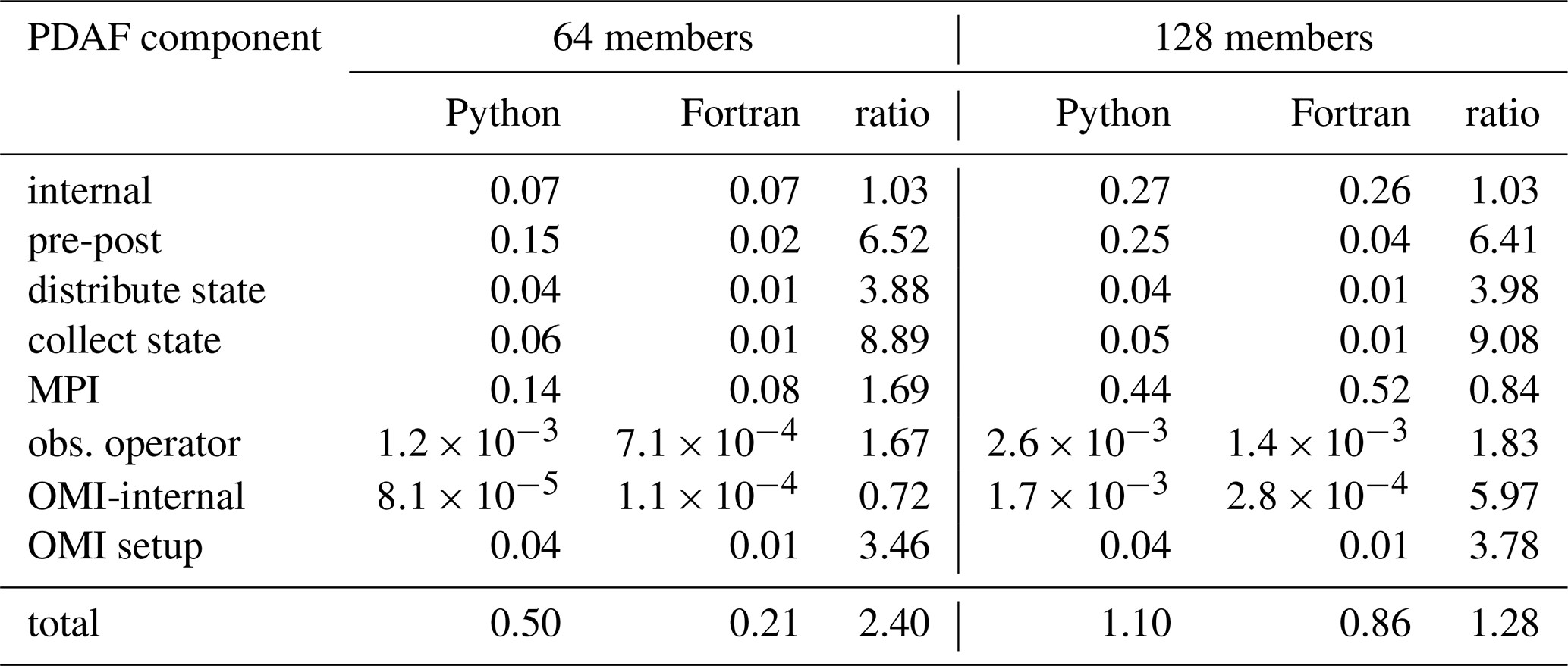
As both numerical computation and user-supplied functions can be sensitive to the number of ensemble members, we further compare the computational time for different ensemble members with 257×257 grid points observed by every 8 grid points. As shown in Table 4, the ETKF takes longer computational time for a larger ensemble. Consistent with other experiments and as expected, the internal PDAF operations take similar computational time between Fortran-based PDAF and Python-based pyPDAF. For all user-supplied functions, compared to the pure Fortran implementation, the pyPDAF leads to increased computational time. The overhead depends on the specific implementation of each function. For example, in the state vector collection and distribution, even though the computational cost should be theoretically proportional to the ensemble size, the overall overhead is stable regardless of the ensemble size. In the pre- and post-processing functions, the overhead relative to the Fortran implementation gets smaller with increased ensemble size as the numerical computations take a higher proportion of the total computational time. The effect of increased ensemble size is also revealed in the observation-related functions. In both the user-supplied function for the observation operator and the internal PDAFomi functions, the computational time increases with the ensemble size. In our specific experiment setup, the overhead does not show large differences with different ensemble size for these observation-related functions. Nevertheless, when the overall computational time between the Fortran and pyPDAF implementation is compared, increasing the ensemble size leads to comparatively lower overhead due to increased numerical computations.

We recognise that the exact computational time can be case-specific. For example, we can postulate that, compared to this study, the overhead can be comparatively smaller for computational intensive user-supplied functions where JIT can be used. This could be the case when correlated observation error covariances are used. Even though this study only investigates the commonly used ETKF and LETKF, the relative run times of pure PDAF and pyPDAF should be similar for other global and local filters. This expectation results from the algorithmic similarity of many filters and the fact that the user routines which are coded in Python when using pyPDAF are mainly the same. However, the overhead may also vary depending on the DA algorithms, in particular for variants of 3DVar. These results demonstrate that pyPDAF has the potential to be used with high-dimensional systems with some increased overhead per analysis step.

5 Conclusions

We introduce the Python package pyPDAF, which provides an interface to the Parallel Data Assimilation Framework (PDAF). We outline its implementation and design. pyPDAF allows for a Python-based DA system for models coded in Python or interfaced to Python. Furthermore it allows for the implementation of a Python-based offline DA system where the DA is performed separately from the model and data is exchanged between the model and DA code through files. The pyPDAF package allows one to implement user-supplied functions in Python for flexible code development while the DA system still benefits from PDAF's efficient DA algorithm implementation in Fortran.

Using a CDA setup, we demonstrate that pyPDAF can be used with the Python model MAOOAM. Both strongly coupled data assimilation (SCDA) and weakly coupled data assimilation (WCDA) are demonstrated. Our results confirm that the SCDA performs better than WCDA. The advantage of pyPDAF in terms of the ease of implementation is reflected by a comparison of the number of lines of code by user-supplied functions in the SCDA setup. The pyPDAF implementation consistently uses fewer lines of code showcasing the requirement for a lower implementation effort than PDAF implementation.

Using the SCDA setup, the computational costs of using pyPDAF and a Fortran-only implementation with PDAF are compared. We show that the computational time stays similar for the core DA algorithm executed in PDAF while pyPDAF yields an overhead in user-supplied functions. This overhead is a result of both the Python implementation and the requirement of data conversion between Python and Fortran. These overheads become comparatively smaller when the analysis becomes computationally more intensive with increased spatial resolution or observation density. To mitigate the overhead in domain localisation implementations, we introduced a new module “PDAFlocal” in PDAF such that a DA system using pyPDAF can achieve similar computational cost as a pure Fortran based system. This module is included since the release v2.3 of PDAF and is now also recommended for the Fortran implementation due to the lower implementation effort. We note that JIT compilation or “f2py” can be used with the Python user-supplied functions for computationally intensive tasks to speed up the Python DA system. In the scope of our specific experiment setup, compared with PDAF, our benchmark shows that, depending on the size of the state vector and ensemble, from 28 % to around three times more time (see Tables 2 and 4) is used by pyPDAF with the global filter while only 6 %–13 % more time is required with a domain-localized filter when applying the Python DA system build with pyPDAF in a high-dimensional dynamical system.

We recognise that the computational cost of the pyPDAF and PDAF can vary case-by-case. Our results demonstrate that the additional “PDAFlocal” module was essential to mitigate the computational overhead in the case of domain localisation. When pyPDAF is used for other DA algorithms and applications, potential efficiency gain can be implemented in future releases of both PDAF and pyPDAF as both pyPDAF and PDAF are still under active development and maintenance.

pyPDAF opens the possibility to apply sophisticated efficient parallel ensemble DA to large-scale Python models such as machine learning models. pyPDAF also allows for the construction of efficient offline Python DA systems. In particular, pyPDAF can be integrated to machine learning models as long as the data structures of such models can be converted to the numpy arrays used by pyPDAF. A pyPDAF-based DA system allows users to utilise sophisticated parallel ensemble DA methods. However, a pyPDAF system does not support GPU parallelisation like TorchDA (Cheng et al., 2025), which is designed based on the machine learning framework pyTorch. The TorchDA package may also have limitations for the application of DA on machine learning models implemented by other frameworks.