Coupling the TKE-ACM2 Planetary Boundary Layer Scheme with the Building Effect Parameterization Model

Understanding and modeling the turbulent transport of surface layer fluxes are essential for numerical weather forecasting models. The presence of heterogeneous surface obstacles (buildings) that have dimensions comparable to the model vertical resolution requires further complexity and design in the planetary boundary layer (PBL) scheme. In this study, we develop a numerical method to couple a recently validated PBL scheme, TKE-ACM2, with multi-layer Building Effect Parameterization (BEP) in the Weather Research and Forecasting (WRF) model. Subsequently, the performance of TKE-ACM2+BEP is examined under idealized convective atmospheric conditions with a simplified building layout. Furthermore, its reproducibility is benchmarked with a state-of-the-art large-eddy simulation model, PALM, which explicitly resolves the building aerodynamics. The results indicate that TKE-ACM2+BEP outperforms another operational PBL scheme (Boulac) coupled with BEP by reducing bias in both the potential temperature (θ) and wind speed (u). Following this, real case simulations are conducted for a highly urbanized domain, namely the Pearl River Delta (PRD) region in China. High-resolution wind speed LiDAR observations suggest that TKE-ACM2+BEP reduces overestimation in the lower part of the boundary layer compared with the Bulk method, which lacks an urban scheme, at a LiDAR site located in a densely built environment. In addition, the surface temperature and relative humidity given by TKE-ACM2+BEP at surface stations in urbanized areas are more accurate than those given by TKE-ACM2 without BEP. However, it is revealed that BEP does not always improve the accuracy of the surface wind speed, as it can introduce excessive aerodynamic drag.

1 Introduction

Urbanization is a ubiquitous phenomenon that is widely seen across the globe. The unprecedented rate of urbanization has resulted in more structures being constructed in populated cities, complicating the response of incoming airflow when it encounters building clusters in the urban canopy layer (UCL) and the overlying roughness sub-layer, or RSL (Rotach, 1999). This RSL is characterized by strong turbulence due to the presence of buildings that separate the mean airflow and form the wake region (Cleugh and Grimmond, 2012), and affect the vertical transport of momentum and scalars over urban regions (Roth, 2000). Mesoscale numerical weather prediction models require parameterizations to account for the net sub-grid effects of building obstacles in heavily populated cities. Given that their horizontal resolution is typically 10 to 50 times the street canyon scale (Britter and Hanna, 2003), they cannot explicitly resolve urban aerodynamics. In the widely-used Weather Research and Forecasting (WRF) model (Skamarock et al., 2019), the surface shear stress exerted by any type of ground obstacle can be simply parameterized using well-known Monin-Obukhov similarity theory (MOST) by defining a friction velocity, u_*, in what is known as the “Bulk” scheme (Liu et al., 2006). Studies have determined different roughness lengths, z₀, a prerequisite for u_*, to account for the heterogeneity of land type (Davenport et al., 2000). However, the Bulk scheme has certain limitations, such as poorly representing urban geometry and failing to apply MOST across the entire RSL (Rotach, 1993). Yet the Bulk scheme is commonly used for real-time weather forecasts (Liu et al., 2006) and analyzing the effects of built-up land on land-sea breeze circulations (Lo et al., 2007).

The single-layer urban canopy model (SLUCM) pioneered by Kusaka et al. (2001), Kusaka and Kimura (2004) is a moderately complex urban parameterization scheme in the WRF model that considers the exchange of momentum and energy between the three-dimensional urban surfaces and the atmosphere in idealized infinitely long street canyons. A major drawback of the SLUCM is that only the first model layer experiences the momentum and sensible heat fluxes due to the presence of buildings, which may lead to unrealistically predicted prognostic variables in the upper surface layer over regions of medium- to high-rise building clustering, such as the Pearl River Delta (PRD) region in southern China. In contrast, multi-layer urban canopy models, such as the Building Effects Parameterizations (Martilli et al., 2002, BEP), and BEP coupled with the Building Energy Model (Salamanca and Martilli, 2010, BEP+BEM), have a higher hierarchy in urban effect parameterizations because of their ability to recognize vertically varying interactions between the atmosphere and buildings (Chen et al., 2011). Besides the direct effect of buildings on the atmosphere dynamics and thermodynamics, BEP$/$BEP+BEM offer modifications to two length scales in the dissipation term of the prognostic turbulent kinetic energy (TKE) equation (Martilli et al., 2002) to account for the altered vortex size. Studies have revealed that meteorological fields and urban heat island effects can be better reproduced using BEP$/$BEP+BEM worldwide, such as in Hong Kong (Wang et al., 2017), Barcelona (Ribeiro et al., 2021), and Bolzano (Pappaccogli et al., 2021).

However, multi-layer BEP$/$BEP+BEM models are adopted less widely than the Bulk scheme or SLUCM because they have only been tentatively coupled to a few planetary boundary layer (PBL) schemes (e.g., Boulac (Bougeault and Lacarrere, 1989), MYJ (Janjić, 1994), and YSU (Hong et al., 2006) added recently by Hendricks et al. (2020)). This is primarily due to the challenges associated with incorporating the transformation of mean kinetic energy into TKE within a first-order closure PBL scheme, such as the YSU scheme. As a result, the eddy diffusivity can only be adjusted in response to surface fluxes, limiting its ability to account for the generation and dissipation of TKE through other boundary layer processes, such as the generation of TKE by wind shear and buoyancy. Additionally, the other two PBL schemes (MYJ and Boulac) model the vertical mixing of momentum between two adjacent layers, but lack the non-local mixing driven by large-scale eddies under convective conditions. For instance, Coniglio et al. (2013) reported that MYJ produces PBLs that are too shallow and moist in the evening, and Xie et al. (2012) found that the PBL height diagnosed by Boulac may be too short to be realistic. Considering that particular PBL schemes may be preferable for different regional and seasonal simulations (García-Díez et al., 2013), there is a need to couple BEP$/$BEP+BEM with other WRF PBL schemes (Martilli et al., 2009), especially a scheme featuring a non-local transport component under convective conditions.

PBL schemes that redistribute surface fluxes and calculate vertical mixing are important to the accurate depiction of meteorological conditions (Xie and Fung, 2014; Wang and Hu, 2021). A number of comparative studies have shown the superiority of non-local PBL schemes over local schemes during convective periods when the uprising plume size is comparable to the vertical grid resolution (Arregocés et al., 2021; Banks et al., 2016; Hu et al., 2010; Xie et al., 2012; Xie and Fung, 2014). With the growing affordability of increased CPU time, recent studies using higher-order turbulence closure models have shown substantial improvements in wind speed and temperature predictions under complex atmospheric conditions compared with first-order schemes (Chen et al., 2022; Olson et al., 2019; Zonato et al., 2022).

The TKE-ACM2 PBL scheme (Zhang et al., 2024) is a recently developed 1.5-order scheme featuring a non-local transport component based on the transilient matrix approach adopted from Pleim (2007a, b). Zhang et al. (2024) evaluated the model's performance by comparing it with measurements obtained by LiDAR units and surface stations, classified as urban or non-urban according to the landuse of the nearest model cell during preprocessing. They showed that the TKE-ACM2 outperformed two other operational PBL schemes, Boulac (Bougeault and Lacarrere, 1989) and ACM2 (Pleim, 2007b), in simulating the vertical profiles of wind speeds. However, overestimated wind speeds persisted throughout the entire surface layer at stations classified as urban type, probably due to the discrepancy resulting from the Bulk parameterization of surface layer fluxes. Therefore, the present paper aims to further improve the application of TKE-ACM2 in urbanized areas by:

1. formulating a numerical method to couple the TKE-ACM2 PBL scheme with the multi-layer BEP model;

2. validating the coupled models in a simplified building layout scenario under different idealized initial and bottom boundary conditions by benchmarking against a finer-scale and building-resolving computational fluid dynamics model, such as the large-eddy simulation (LES) model; and

3. applying the coupled models in real case simulations over densely built areas, such as the PRD region, where the land occupied by medium- to high-rise buildings accounts for a great proportion of the total urbanized area. Subsequently, the performance of TKE-ACM2 coupled with BEP is evaluated in terms of the wind speeds using measurements from a network of high-resolution wind speed LiDAR units.

Section 2 describes the model development, the LES tool used to validate TKE-ACM2+BEP in an idealized urban morphology setup, the observational instrument, and the Local Climate Zones (LCZ) used for real case simulations. Section 3 evaluates the performance of the TKE-ACM2 and Boulac PBL schemes coupled with BEP by comparing them with LES under various idealized convective conditions over a simplified staggered building layout, using Bulk methods as the reference. Section 4 presents the effects of TKE-ACM2 with/without BEP on potential temperature (θ) and wind speed (U) profiles in real case simulations, highlighting the differences between TKE-ACM2 and Boulac.

2 Methodology and materials

2.1 Numerical method for coupling TKE-ACM2 and BEP

The formulation and validation of the TKE-ACM2 PBL scheme were detailed by Zhang et al. (2024). The remarkable difference between TKE-ACM2 and its predecessor ACM2 (Pleim, 2007b) is that TKE-ACM2 adopts a 1.5-order turbulence closure model to calculate the eddy diffusivity/viscosity, rather than using prescribed profiles for different stabilities. Moreover, TKE-ACM2 differs from Boulac in that the non-local transport of both the momentum and scalars under convective conditions is reflected using the transilient matrix approach in TKE-ACM2, whereas Boulac parameterizes the transport of momentum based on the local gradient only and uses the counter-gradient method for potential temperature transport, which is not energy conserving. Following Pleim (2007b), the governing equation balancing the tendency terms for zonal (u) or meridional (v) wind, potential temperature (θ), and water vapor mixing ratio (q) with the vertical gradients of fluxes is

$$\begin{array}{}\text{(1)}& {\displaystyle \frac{\partial \mathit{\zeta }}{\partial t}}=-{\displaystyle \frac{\partial }{\partial z}}\stackrel{\mathrm{‾}}{w^{\prime }{\mathit{\zeta }}^{\prime }}\end{array}$$

where $\mathit{\zeta }\in \mathit{\{}u,v,\mathit{\theta },q\mathit{\}}$. The vertical turbulent fluxes comprising the local gradient transport and transilient non-local transport are parameterized as

$$\begin{array}{}\text{(2)}& {\stackrel{\mathrm{‾}}{w^{\prime }{\mathit{\zeta }}^{\prime }}}_I=-K_{\mathit{\zeta },I}{\displaystyle \frac{S_I({\mathit{\zeta }}_{i+\mathrm{1}}^n-{\mathit{\zeta }}_i^n)}{V_i\mathrm{\Delta }{z}_I}}+\mathrm{Mu}\left(h-z_I\right)\left({\mathit{\zeta }}_{\mathrm{1}}^n-{\mathit{\zeta }}_i^n\right)\end{array}$$

where the subscripts i (I) denote variables located at half (full) sigma levels, K_ζ=K_h is the eddy diffusivity for $\mathit{\zeta }\in \mathit{\{}\mathit{\theta },q\mathit{\}}$ and K_ζ=K_m is the eddy viscosity for $\mathit{\zeta }\in \mathit{\{}u,v\mathit{\}}$, V and S are the volume and surface fractions not occupied by buildings, Mu is the upward convective transport rate, and h is the boundary layer height. Adding the environmental forcing acting on multiple model levels, the discretized form of Eq. (1) is written as

$$\begin{array}{}\text{(3)}& \begin{array}{rl}& {\displaystyle \frac{{\mathit{\zeta }}_i^{n+\mathrm{1}}-{\mathit{\zeta }}_i^n}{\mathrm{\Delta }t}}=\underset{\text{upward convective transport}}{\underbrace{f_{\text{conv }}\mathrm{Mu}{\mathit{\zeta }}_{\mathrm{1}}^n}}\\ & -\underset{\text{donward transport}}{\underbrace{f_{\text{conv }}{\mathrm{Md}}_i{\mathit{\zeta }}_i^n+f_{\text{conv }}{\mathrm{Md}}_{i+\mathrm{1}}{\mathit{\zeta }}_{i+\mathrm{1}}^n{\displaystyle \frac{\mathrm{\Delta }{z}_{i+\mathrm{1}}}{\mathrm{\Delta }{z}_i}}}}\\ & +\underset{\text{local transport}}{\underbrace{\left(\mathrm{1}-f_{\text{conv }}\right){\displaystyle \frac{\mathrm{1}}{V_i\mathrm{\Delta }{z}_i}}\left[\begin{array}{c}{S}_I{\displaystyle \frac{K_{\mathit{\zeta },I}\left({\mathit{\zeta }}_{i+\mathrm{1}}^n-{\mathit{\zeta }}_i^n\right)}{\mathrm{\Delta }{z}_I}}\\ -S_{I-\mathrm{1}}{\displaystyle \frac{K_{\mathit{\zeta },I-\mathrm{1}}\left({\mathit{\zeta }}_i^n-{\mathit{\zeta }}_{i-\mathrm{1}}^n\right)}{\mathrm{\Delta }{z}_{I-\mathrm{1}}}}\end{array}\right]}}\\ & +\underset{\text{env. forcing}}{\underbrace{{\displaystyle \frac{F_i}{\mathrm{\Delta }{z}_i}}}}\end{array}\end{array}$$

where the superscript n+1 indicates the time forwarding by a timestep (Δt), f_conv is the ratio that partitions the local and non-local transport, Md is the downward compensatory transport rate, and Δz is the vertical resolution. The original formulations of f_conv, Mu, and Md were detailed by Pleim (2007b), and the model sensitivity to some of these parameters was given by Zhang et al. (2024). The last term on the RHS of Eq. (3), denoting collective forcing from both the urban area and non-urban (natural) area for the first model layer (i=1), is computed using the weighted sum approach if the urban fraction (Urb) is less than 1; i.e., $F_{\mathrm{1}}=(\mathrm{1}-\mathrm{Urb})F_{\mathrm{natural},\mathrm{1}}+\mathrm{Urb}{F}_{\mathrm{urban},\mathrm{1}}$. For model layers i>1, the environmental forcing F_i is UrbF_urban,i alone. Readers interested in the parameterization of F_urban are referred to the work of Martilli et al. (2002). Effectively, F_i is computed in the subroutine phys/module_sf_bep.F, resulting in the term $F_i/\mathrm{\Delta }{z}_i$ being written as the combination of implicit (A_i) and explicit (B_i) parts which are outputs from BEP; i.e., $F_i/\mathrm{\Delta }{z}_i=A_i{\mathit{\zeta }}_i+B_i$ for matrix inversion.

The prognostic equation for TKE (e) in TKE-ACM2 coupled with BEP is identical to that given by Zhang et al. (2024), but the parameterizations of each source/sink term are modified mainly to account for (1) the external TKE source converted from mean kinetic energy when flow separates and (2) the altered characteristic length scale for eddies in the wake region due to buildings. According to Bougeault and Lacarrere (1989) and Makedonas et al. (2021), the prognostic equation for e considering the building effects is

$$\begin{array}{}\text{(4)}& {\displaystyle \frac{\partial e}{\partial t}}=-{\displaystyle \frac{\mathrm{1}}{\mathit{\rho }}}{\displaystyle \frac{\partial }{\partial z}}\mathit{\rho }\stackrel{\mathrm{‾}}{w^{\prime }e}-\stackrel{\mathrm{‾}}{u^{\prime }{w}^{\prime }}{\displaystyle \frac{\partial u}{\partial z}}-\stackrel{\mathrm{‾}}{v^{\prime }{w}^{\prime }}{\displaystyle \frac{\partial v}{\partial z}}+\mathit{\beta }\stackrel{\mathrm{‾}}{w^{\prime }{\mathit{\theta }}^{\prime }}-\mathit{ϵ}+{\displaystyle \frac{\partial F}{\partial z}}\end{array}$$

where ρ is the density of air, β is the buoyancy coefficient, and $\mathit{ϵ}=\mathit{\rho }{C}_{\mathit{ϵ}}{e}^{\mathrm{3}/\mathrm{2}}/l_{\mathit{ϵ}}$ represents the TKE dissipation rate where $C_{\mathit{ϵ}}=\mathrm{1}/\mathrm{1.4}$ is an empirical constant and l_ϵ corresponds to the characteristic length of energy-containing eddies. The turbulent fluxes for momentum and heat are already given in Eq. (2). $\partial F/\partial z$ representing TKE generated by buildings can be written in a similar manner to momentum $/$ heat as Ae+B and is readily available from the BEP module in WRF. Assuming that the vertical turbulent transport of TKE mimics that of passive scalars, the parameterization of $\stackrel{\mathrm{‾}}{w^{\prime }e}$ is expressed similarly to Eq. (2) as

$$\begin{array}{}\text{(5)}& {\stackrel{\mathrm{‾}}{w^{\prime }e}}_I=-K_{\mathrm{e},I}{\displaystyle \frac{S_I(e_{i+\mathrm{1}}-e_i)}{V_i\mathrm{\Delta }{z}_I}}+\mathrm{Mu}\left(h-z_I\right)\left(e_{\mathrm{1}}-e_i\right)\end{array}$$

The eddy diffusivity is equal in magnitude for scalars (K_h) and TKE (K_e) and is related to eddy viscosity (K_m) through the turbulent Prandtl number (Pr_t), which is a key parameter pertinent to heat transfer (Li, 2019):

$$\begin{array}{}\text{(6)}& K_{\mathrm{e}}=K_{\mathrm{h}}=K_{\mathrm{m}}/P{r}_t\end{array}$$

where $K_{\mathrm{m}}=C_K{l}_k{e}^{\mathrm{1}/\mathrm{2}}$, C_K is a 𝒪(1) empirical constant, the parameterization of Pr_t is consistent with that presented by Zhang et al. (2024), which follows Businger et al. (1971), and the length scale l_k is modified from that calculated by Bougeault and Lacarrere (1989) (l_k,old) because the buildings generate vortices whose size of l_build. is comparable to the building spatial dimension (typically the building height), according to Martilli et al. (2002). This is expressed by

$$\begin{array}{}\text{(7)}& {\displaystyle \frac{\mathrm{1}}{l_k}}={\displaystyle \frac{\mathrm{1}}{l_{\text{old }}}}+{\displaystyle \frac{\mathrm{1}}{l_{\mathrm{build}.}}}\end{array}$$

The same modification applies to l_ϵ, which suggests an enhanced dissipation of TKE (Martilli et al., 2002). Ultimately, solving Eq. (3) is straightforward using the computed K_ζ values derived from Eq. (6). The finite difference method used to obtain numerical solutions for Eq. (3) is described in detail in Appendix A.

2.2 Large-eddy simulation model

Prior to implementing the TKE-ACM2 PBL scheme coupled with BEP in real case simulations, we performed idealized simulations using prescribed surface heat fluxes along with simplified urban morphology. We then benchmarked the results against those of PALM, a state-of-the-art LES model capable of resolving building aerodynamics. The PALM model (Maronga et al., 2015; Raasch and Schröter, 2001) is a non-hydrostatic incompressible Navier-Stokes equation solver that has been rigorously evaluated against experiments. It thus often serves as a benchmark for deriving new parameterizations of boundary layer turbulent mixing in mesoscale weather forecasting models. PALM uses a 1.5-order turbulence closure model for solving isotropic turbulence in three dimensions simultaneously. One salient advantage of PALM over other wall-resolved LES models is that PALM adopts MOST between the solid boundary and the first model layer above, which greatly increases computational efficiency while preserving accuracy in the context that the mesoscale model has Δz∈ {𝒪(10) m, 𝒪(1000) m}.

2.3 Idealized simulation setup

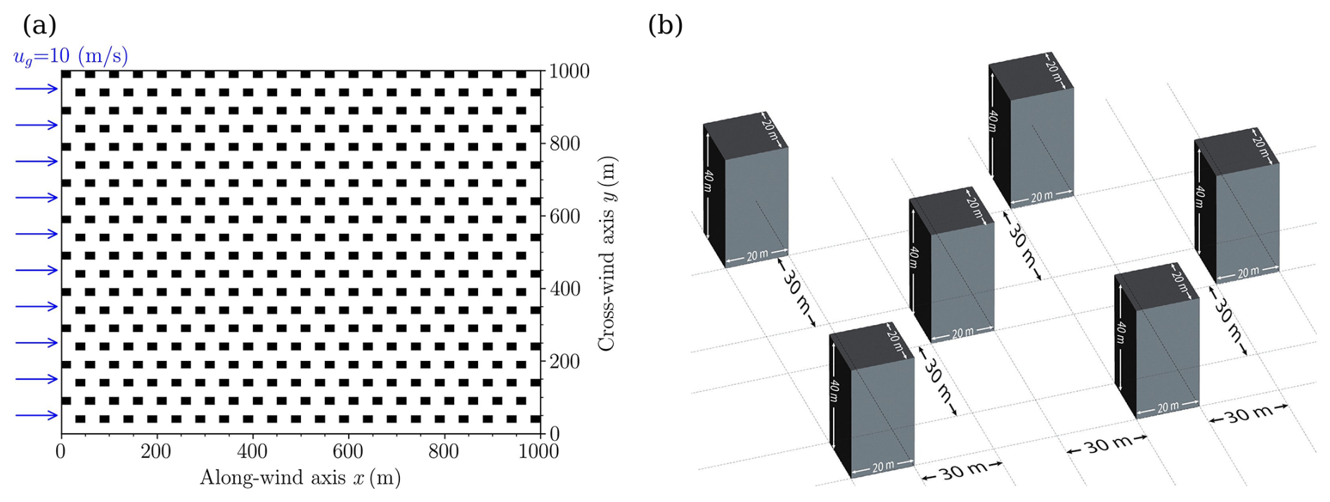
A 1 km long by 1 km wide by 1.5 km high domain with equidistant spatial resolutions $\mathrm{\Delta }x=\mathrm{\Delta }y=\mathrm{\Delta }z=\mathrm{5}$ m and staggered building arrays was set up for the PALM model. Figure 1 provides a plan view of the domain setup and urban morphology configuration, where buildings have a cross-section of 20 m square and a height of 40 m and the windward wall is perpendicular to the upwind flow. The prescribed height of building arrays is justified by the fact that it is commonly seen in Hong Kong according to Kwok et al. (2020). The street width in both horizontal directions is set as 30 m to align with a moderately densely built environment. The street width to building width ratio $(\mathrm{2}/\mathrm{3})$ is deemed an “open” exposure in urban areas and has good representativity in Hong Kong. Unlike PALM, which operates at a building-resolving scale, WRF+BEP runs at a building-parameterized scale ($\mathrm{\Delta }x=\mathrm{\Delta }y=\mathrm{1}$ km), where explicitly resolving building aerodynamics is impractical. We thus prescribed the urban morphological parameters to be consistent with PALM in the WRF+BEP look-up table required for BEP. The WRF+BEP domain was horizontally extended to 20 km by 20 km to capture large-scale thermal plumes in the convective flow (Schmidt and Schumann, 1989). The domain height remained 1.5 km, but with a slightly coarser vertical resolution of Δz=12.5 m.

Figure 1 (a) Plan view of domain setup; (b) configuration of the urban morphology.

The initial condition was set $u_{\mathrm{0}}=u_{\mathrm{g}}=\mathrm{10}$ m s⁻¹ with a uniform distribution along the vertical direction and $v_{\mathrm{0}}=v_{\mathrm{g}}=\mathrm{0}$ m s⁻¹, where u_g and v_g are geostrophic winds with the Coriolis parameter being 10⁻⁴ s⁻¹. Two initial potential temperature profiles were selected for the idealized simulations, one corresponding to a moderately convective atmosphere (${\stackrel{\mathrm{‾}}{w^{\prime }{\mathit{\theta }}^{\prime }}}_{\mathrm{0}}=\mathrm{0.10}$ K m⁻¹ s⁻¹, denoted as Case 10WC) with no capping inversion and the other representing strongly convective atmospheric stability (${\stackrel{\mathrm{‾}}{w^{\prime }{\mathit{\theta }}^{\prime }}}_{\mathrm{0}}=\mathrm{0.24}$ K m⁻¹ s⁻¹, denoted as Case 24SC) with a strong capping inversion to limit the growth of the boundary layer. The analytical expressions of two initial θ profiles are given below, where $\partial \mathit{\theta }/\partial z$ in the free atmosphere is $\mathrm{1}\mathrm{K}/\mathrm{100}$ m in both cases:

$$\begin{array}{}\text{(8)}& \begin{array}{rl}& \mathrm{Case}\mathrm{10}\mathrm{WC}:{\mathit{\theta }}_{\mathrm{0}}\left(z\right)=\\ & \left\{\begin{array}{l}\mathrm{300}\mathrm{K},z<\mathrm{600}\mathrm{m}\\ \mathrm{300}\mathrm{K}+\mathrm{1}/\mathrm{100}(z-\mathrm{600})\mathrm{K},z\ge \mathrm{600}\mathrm{m}\end{array}\right.\end{array}\end{array}$$

and

$$\begin{array}{}\text{(9)}& \begin{array}{rl}& \mathrm{Case}\mathrm{24}\mathrm{SC}:{\mathit{\theta }}_{\mathrm{0}}\left(z\right)=\\ & \left\{\begin{array}{l}\mathrm{300}\mathrm{K},z<\mathrm{600}\mathrm{m}\\ \mathrm{300}\mathrm{K}+\mathrm{6}/\mathrm{100}(z-\mathrm{600}),\mathrm{600}\mathrm{m}\le z<\mathrm{800}\mathrm{m}\\ \mathrm{300}\mathrm{K}+\mathrm{6}/\mathrm{100}(\mathrm{800}-\mathrm{600})\mathrm{K}+\mathrm{1}/\mathrm{100}(z-\mathrm{800})\mathrm{K},z\ge \mathrm{800}\mathrm{m}\end{array}\right.\end{array}\end{array}$$

All boundary conditions were identically set in the PALM and WRF+BEP simulations. The lateral boundary conditions for the along-wind direction (x) and cross-wind direction (y) were set as periodic to simulate an infinitely long urban fetch. The bottom boundary conditions for heat were reflected by different values of ${\stackrel{\mathrm{‾}}{w^{\prime }{\mathit{\theta }}^{\prime }}}_{\mathrm{0}}$ and a free-slip condition was set for the top boundary condition. The microscale roughness length (z₀) was set as 0.01 m for both the ground and roof in PALM, ensuring consistency with the value in the look-up table used for WRF+BEP. The runtime parameters needed to obtain meaningful results (Ayotte et al., 1996; Nazarian et al., 2020) for PALM and WRF+BEP are described in more detail in Sect. 3. The temperatures of solid surfaces (roofs, walls, and streets) in PALM and WRF+BEP are prescribed as 300 K.

2.4 Real case simulation materials

2.4.1 Landuse data and wind LiDAR observation network

This study adopted the 17-class LCZ classification scheme (Demuzere et al., 2022) to more accurately capture the highly variable urban morphology within the domain of interest. The distribution of LCZ 1 to 10 (urban) grids and LCZ A to G (non-urban) grids is depicted in Fig. 2c. Each class is defined in Table B1 (Appendix B).

A wind speed Doppler LiDAR network (see Fig. 2d) has been operational in Hong Kong since March 2020, continuously monitoring wind conditions and playing a crucial role in validating regional downscaling results. The network comprises three WindCube 100S LiDAR units manufactured by Vaisala. Each unit measures the vertical profile of the wind speed at an elevation angle of 90°. The units measure 25 m intervals starting from 50 m above ground level, with an accuracy of <0.5 m s⁻¹ for wind speed and 2° for wind direction. Although each LiDAR outputs data at a frequency of 1 Hz, measurements are averaged hourly and archived due to storage limitations. We represent the land cover type of each LiDAR unit using the LCZ classification associated with the nearest model grid following Ribeiro et al. (2021).

The LiDAR unit at the Hong Kong University of Science and Technology Supersite (USTSS_LCZ5) is located on the east coast of Kowloon Island (22.333° N, 114.267° E), where the nearest model grid center falls within LCZ 5 (open mid-rise). The second LiDAR, installed on the southeastern peninsula of Hong Kong Island (Hok Tsui, 22.209° N, 114.253° E), is surrounded by natural vegetation and referred to as HT_rural. Lastly, the LiDAR at King's Park (22.312° N, 114.170° E) in downtown Kowloon, where the average building height is 60 m (Kwok et al., 2020), is located within an LCZ 1 model grid (compact high-rise), and designated as KP_LCZ1.

In addition to profiler-type observations, we also used measurements of surface meteorological variables, including the 10 m wind speed (U₁₀), 2 m temperature (T₂), and 2 m relative humidity (RH₂), retrieved from the Global Telecommunication System. The coordinates corresponding to each automated weather station (AWS) are retrieved from the little-r formatted files and outlined in the figures in the Supplement, e.g., Figs. S6 to S98. The elevation of each AWS is 10 m above the ground. The landuse type of each AWS and LiDAR unit is identified using the nearest model grid point, which is also outlined in the figures in the Supplement. All observational data presented in this work is 1 h averaged. The AWS dataset comprises a total of 13 urban stations characterized by LCZ classes 1 to 10, along with 10 stations situated on water surfaces, and 8 rural stations on land. The distribution of surface stations across specific LCZ classes is provided in Table B1 (Appendix B).

2.4.2 Configuration of real case simulations

A four-nested domain having a parent domain grid ratio of 1:3 and a reference latitude of 28.5° N and longitude of 114° E (Fig. 2a) was adopted. The coarsest domain (D1) with $\mathrm{\Delta }x=\mathrm{\Delta }y=\mathrm{27}$ km spanned 283 grid points in the East–West direction and 184 grid points in the North–South direction, covering the entirety of China. The finest domain (D4), with a horizontal resolution of 1 km, focused on the PRD region, which encompasses heavily populated and densely built mega-cities including Hong Kong (7.3 million people as of 2021), Shenzhen (17.6 million), and Guangzhou (18.7 million). The surface stations and high-resolution wind speed LiDAR locations deployed in D4 are highlighted in Fig. 2d. 30 d simulations were performed from 12:00 UTC+0 on 18 July to 12:00 UTC+0 on 18 August of year 2022. The integration was performed using a one-day overlap for the spin-up between two consecutive four-day segments.

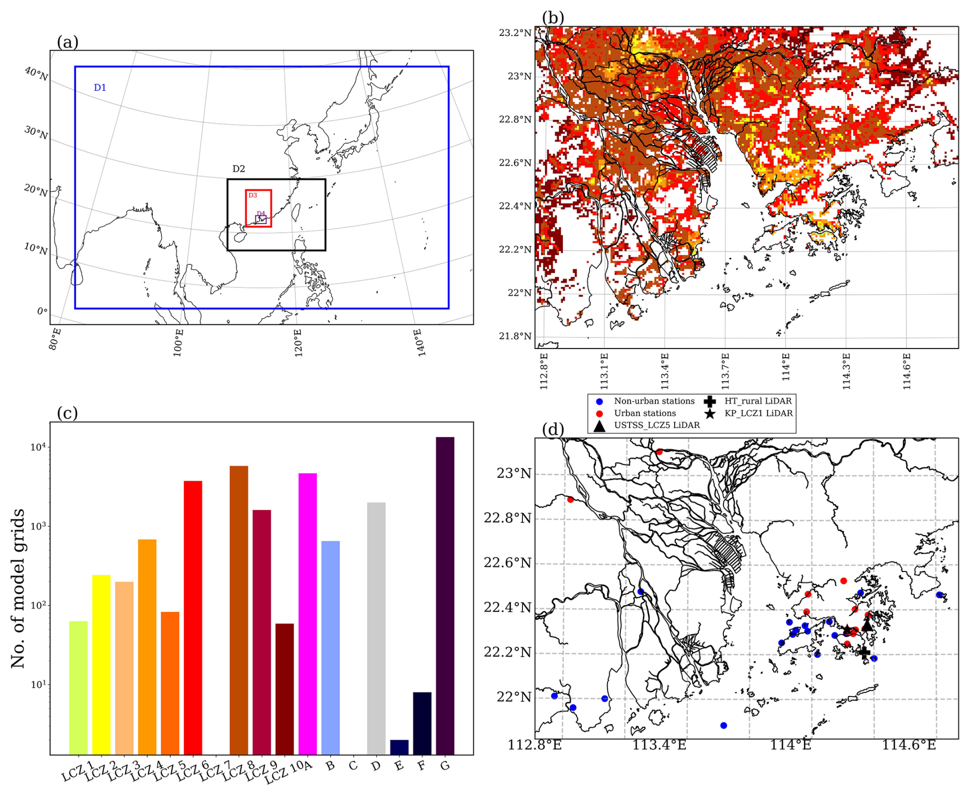
Figure 2 (a) Four-nested domain; (b) LCZ urban grids (LCZ 1 to 10) for domain 4 having 1 km resolution with the color scheme represented in panel (c); (c) LCZ distribution in D4; (d) distributions of surface stations and wind speed LiDAR.

The configuration of real case simulations is outlined in Table B2. We configured the WRF eta levels such that multiple vertical model grids intersected the UCL and RSL. Thus, the variability of wind speeds was better represented by BEP where buildings were taller than the first above-ground full eta level. The lowest six half eta levels corresponded to approximately 9, 28, 49, 71, 96, and 122 m above ground level (a.g.l.). We used NCEP GFS analysis data at 6-hourly input intervals to provide the initial and lateral boundary conditions.

Identical physics schemes were chosen in the four simulations: the unified Noah scheme (Chen and Dudhia, 2001) for the land-surface model, WSM 3-class simple ice scheme (Hong et al., 2004) for microphysics, RRTMG scheme (Iacono et al., 2008) for longwave/shortwave radiation, and Grell-Freitas ensemble scheme (Gall et al., 2013) for cumulus. The TKE-ACM2 PBL scheme was coupled with the BEP UCM (referred to as TKE-ACM2+BEP) and evaluated alongside the TKE-ACM2 scheme in isolation (TKE-ACM2+Bulk), where the surface layer fluxes were computed using the Noah land-surface model. The Boulac PBL scheme underwent the same evaluation, being coupled with the BEP UCM (Boulac+BEP) and assessed in isolation with the Noah land surface model (Boulac+Bulk). The look-up table for LCZ class properties that provided crucial parameters, including the impervious fraction and building height distribution, is included in the Supplement to the present work, archived in Zhang (2024).

3 Idealized simulations results

3.1 Turbulence characteristics and runtime parameters

Nazarian et al. (2020) showed the importance of choosing appropriate runtime parameters for LES in a neutral atmosphere over building arrays. As the present study adopted two convective scenarios in a similar urbanized domain, extra attention needs to be paid to thermal characteristics in determining the runtime parameters. As revealed by Ayotte et al. (1996) and Shin and Dudhia (2016), the durations of simulations can be determined by examining the temporal variation of turbulence statistics. We first examined the time required for LES to reach a quasi-equilibrium state by investigating the variation of the maximum resolved TKE (e_res.) and the absolute value of the maximum vertical velocity ($\left|w_{\max }\right|$), shown in Fig. 3.

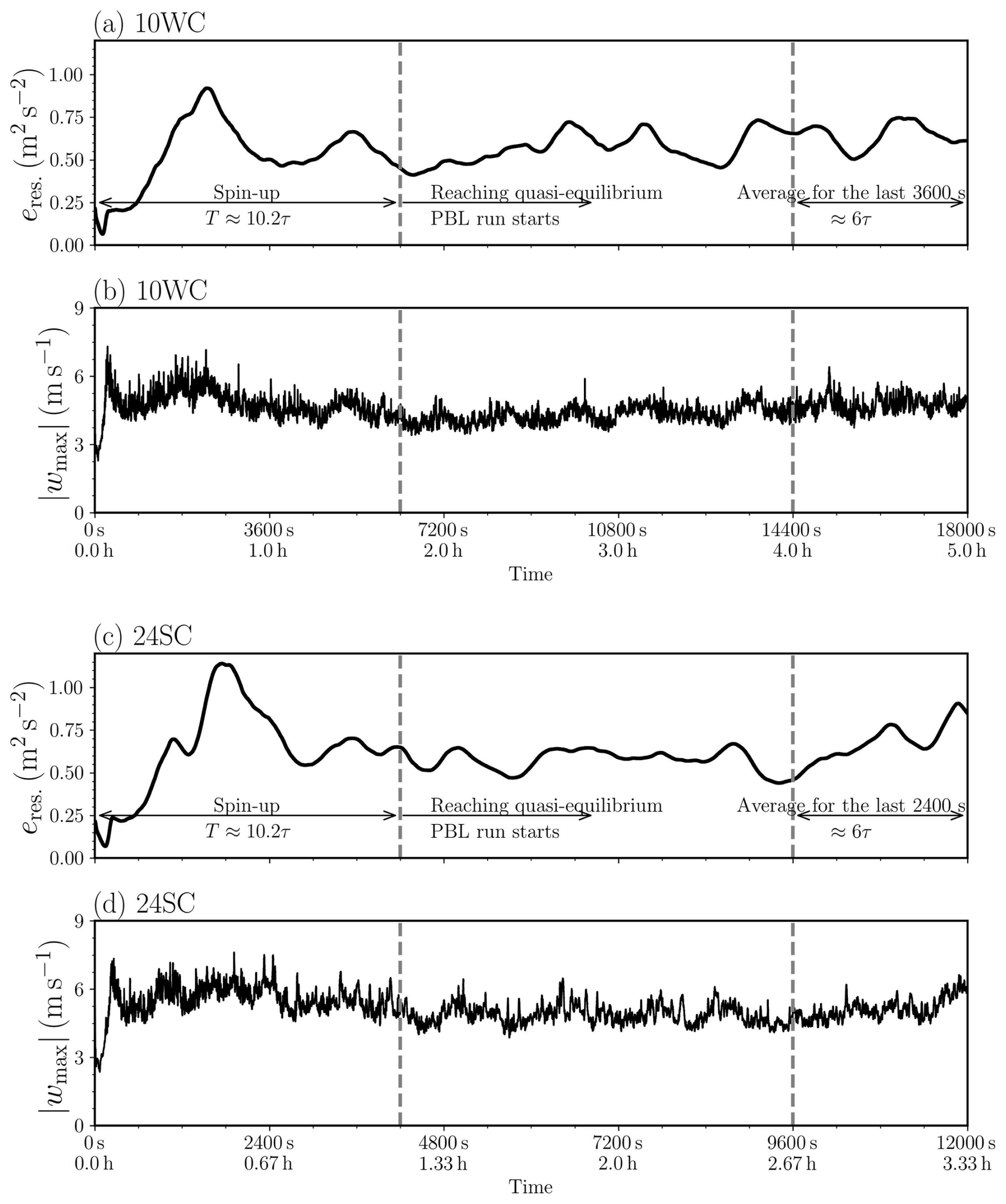
Figure 3 (a) Time series of e_res. for Case 10WC; (b) time series of $\left|w_{\max }\right|$ for Case 10WC; (c) same as (a) but for Case 24SC; (d) same as (b) but for Case 24SC.

Quasi-equilibrium was achieved in the two LES cases after approximately 10.2 convective turnover times (τ), where $\mathit{\tau }=h/w^{*}$, and $w^{*}=(\mathit{\beta }{\stackrel{\mathrm{‾}}{w^{\prime }{\mathit{\theta }}^{\prime }}}_{\mathrm{0}}h{)}^{\mathrm{1}/\mathrm{3}}$ represents the convective velocity scale. The duration of 10.2 large-eddy turnover times was considered a reasonable indicator of well-developed dynamic fields over the domain with buildings, especially compared with other studies that have used factors of 5 (Ayotte et al., 1996; Pleim, 2007b; Zhang et al., 2024) and 6 (Shin and Dudhia, 2016) for flat domains.

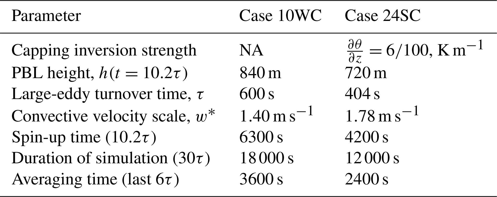
The horizontal averages of the velocity and potential temperature fields were calculated at 10.2τ and served as initial conditions for driving mesoscale WRF simulations for an additional 20τ. Subsequently, the results from the final 6τ, corresponding to either 3600 s or 2400 s, were averaged both horizontally and temporally. Table 1 summarizes the key turbulence characteristics of the convective flow and the runtime parameters.

Table 1 Turbulence characteristics and runtime parameters. NA = Not applicable.

The horizontally averaged u and θ profiles during the last 6τ are displayed in Fig. 4 and the turbulent fluxes from PALM and computed from WRF PBL schemes are contrasted in Fig. 5. The total turbulent momentum flux in Boulac was simply computed using the local gradient as $-K_{\mathrm{m}}\partial u/\partial z$ whereas the turbulent heat flux required the addition of the counter-gradient flux shown as $-K_{\mathrm{h}}(\partial \mathit{\theta }/\partial z-\mathit{\gamma })$. The root-mean-square-error (RMSE) for first-order moments u,θ and second-order moments $\stackrel{\mathrm{‾}}{w^{\prime }{\mathit{\theta }}^{\prime }},\stackrel{\mathrm{‾}}{w^{\prime }{u}^{\prime }}$ calculated below the PBL height is displayed in Fig. 6.

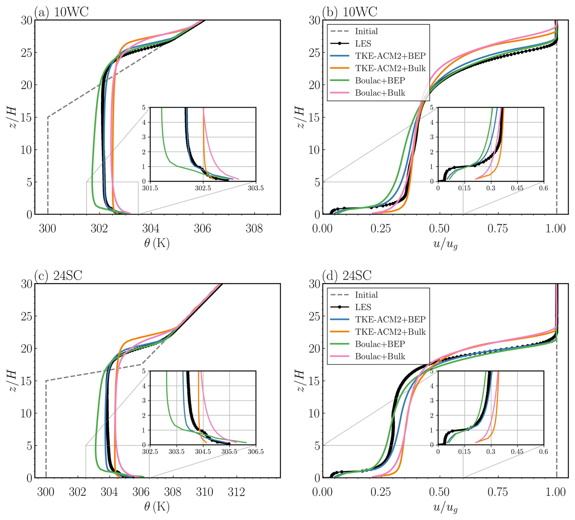
Figure 4 (a) Horizontally averaged θ profile during the last 6τ for Case 10WC; (b) horizontally averaged u profile normalized by u_g=10 m s⁻¹ during the last 6τ for Case 10WC; (c) same as (a) but for Case 24SC; (d) same as (b) but for Case 24SC. The gray dashed lines represent the initial conditions. The black dotted line shows the LES results. The solid blue, orange, green, and pink lines represent the results for TKE-ACM2+BEP, TKE-ACM2+Bulk, Boulac+BEP, and Boulac+Bulk, respectively.

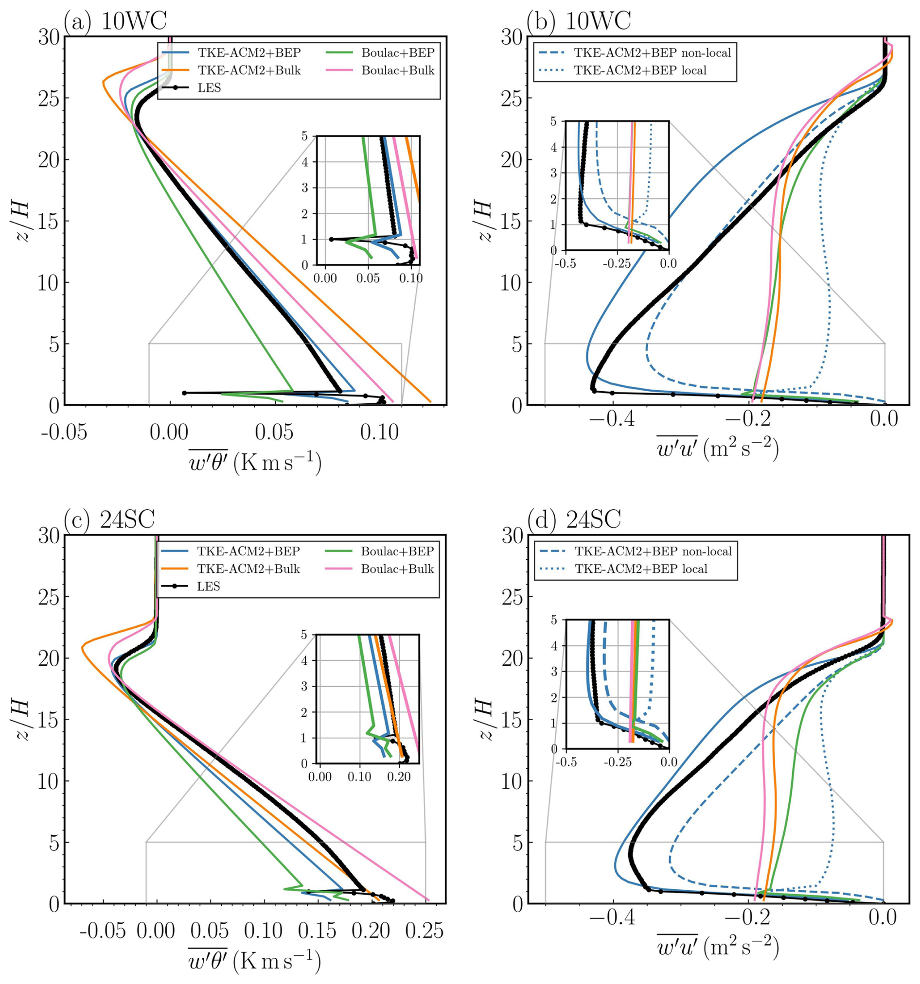
Figure 5 (a) Horizontally averaged $\stackrel{\mathrm{‾}}{w^{\prime }{\mathit{\theta }}^{\prime }}$ profile during the last 6τ for Case 10WC; (b) horizontally averaged $\stackrel{\mathrm{‾}}{w^{\prime }{u}^{\prime }}$ profile during the last 6τ for Case 10WC; (c) same as (a) but for Case 24SC; (d) same as (b) but for Case 24SC. The black dotted line shows the LES results. The solid blue, orange, green, and pink lines represent results for TKE-ACM2+BEP, TKE-ACM2+Bulk, Boulac+BEP, and Boulac+Bulk, respectively. The blue dashed and blue dotted lines represent the non-local and local turbulent momentum fluxes of TKE-ACM2+BEP, respectively. The insets show magnified results for $z/H\le \mathrm{5}$. All y-axes are normalized by the uniform building height H=40 m.

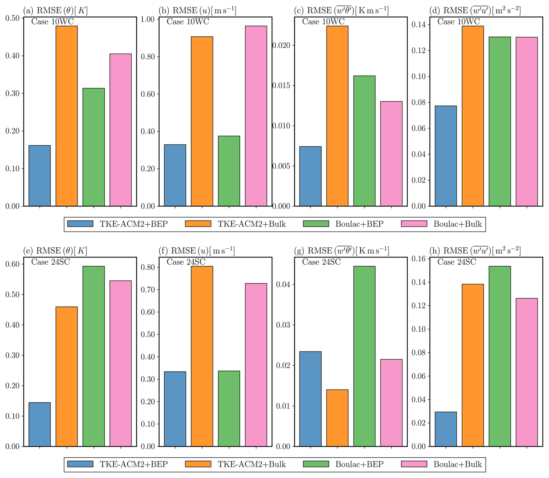
Figure 6 (a–d) RMSEs for θ, u, $\stackrel{\mathrm{‾}}{w^{\prime }{\mathit{\theta }}^{\prime }}$, and $\stackrel{\mathrm{‾}}{w^{\prime }{u}^{\prime }}$, calculated below the PBL height for Case 10WC by taking the LES results as the reference, respectively; (e–h) same as (a)–(d) but for Case 24SC.

3.2 Case 10WC results: vertical profiles of $\mathit{\theta },u,\stackrel{\mathrm{‾}}{w^{\prime }{\mathit{\theta }}^{\prime }}$, and $\stackrel{\mathrm{‾}}{w^{\prime }{u}^{\prime }}$

In Case 10WC, with a moderate surface heat flux, both TKE-ACM2+BEP and Boulac+BEP reproduced the unstable atmosphere below the inertial sub-layer (ISL), which was located at approximately 3H (Fig. 4a). However, Boulac+BEP simulated a warmer bias in θ at the first model layer and a colder bias at roof level, resulting in an excessively unstable UCL. In addition, the cold bias persisted throughout the mixed layer. In contrast, TKE-ACM2+BEP produced a smaller warm bias in the UCL. Furthermore, θ in the overlaying ISL was well reproduced by TKE-ACM2+BEP. A deeper well-mixed boundary layer ($\partial \mathit{\theta }/\partial z\approx \mathrm{0}$) was simulated using TKE-ACM2+BEP, and a discrepancy in the Boulac+BEP results relative to the LES results suggests that the boundary layer became slightly unstable from approximately 10H. Relative to BEP simulations, the Bulk methods produce consistently overestimated θ within the PBL. Figure 4b suggests that PALM simulated a strong wind shear at the roof level, while such an inflection point in the wind speed profile was successfully reproduced by BEP, in contrast with the Bulk simulations, in which the wind shear ($\partial u/\partial z$) was relatively gentle at roof level. The momentum simulated by TKE-ACM2+BEP generally exhibited better agreement with LES than Boulac+BEP, especially within the mixed layer. The most visible negative bias of u in BEP simulations occurred at [1H,5H]. It should be highlighted in Fig. 4b that from the ground level to the top of the UCL, both BEP simulations overestimated the wind speed in contrast to an underestimation in the mixed layer. It thus appears that the BEP parameterization resulted in an underestimation of wind shear at roof level when compared with the LES. The Bulk simulations clearly indicate that the lack of multi-layer parameterization of aerodynamic drag led to overestimation of the wind speed within the UCL.

The heat flux profile in Fig. 5a reveals that the trends of variation were well captured in the two BEP simulations, in that the drastic reduction in heat flux when approaching the roof level from the ground was reproduced. The TKE-ACM2+Bulk simulation produced a heat flux of 0.124 K m s⁻¹ (0.207 K m s⁻¹) at the ground in Case 10WC (Case 24SC) according to Fig. 5a (Fig. 5c), which is approximately 1.17 (0.817) times the magnitudes simulated by Boulac+Bulk. It is important to emphasize that the heat flux forcing caused by urban effects, represented by term (F) in Eq. (3), consists of the heat flux between the vertical surfaces of the building and the air (${\stackrel{\mathrm{‾}}{w^{\prime }{\mathit{\theta }}^{\prime }}}_{\mathrm{vert}}$) as well as the heat flux between the horizontal surfaces and the air (${\stackrel{\mathrm{‾}}{w^{\prime }{\mathit{\theta }}^{\prime }}}_{\mathrm{hor}}$), as noted by Martilli et al. (2002). A scale analysis based on Martilli et al. (2002) (see Eq. 10) reveals that ${\stackrel{\mathrm{‾}}{w^{\prime }{\mathit{\theta }}^{\prime }}}_{\mathrm{vert}}$ is proportional to $-(\mathit{\theta }-{\mathit{\theta }}^{\text{wall}})\mathit{\eta }/c_p\approx -\mathcal{O}\left({\mathrm{10}}^{-\mathrm{5}}\right)\mathrm{\Delta }\mathit{\theta }$, where η is 𝒪(10) and $c_p={\mathrm{10}}^{-\mathrm{6}}$ J m⁻³ K⁻¹.

$$\begin{array}{}\text{(10)}& {\stackrel{\mathrm{‾}}{w^{\prime }{\mathit{\theta }}^{\prime }}}_{i,\mathrm{vert}}=-{\displaystyle \frac{\mathit{\eta }}{\mathit{\rho }{c}_p}}\left[\left({\mathit{\theta }}_i-{\mathit{\theta }}_i^{{\text{West }}^{\text{wall }}}\right)+\left({\mathit{\theta }}_i-{\mathit{\theta }}_i^{{\text{East }}^{\text{wall }}}\right)\right]S_i\end{array}$$

where the superscript of θ^wall indicates the orientation of walls for an exemplary North–South street direction. In contrast, the heat flux at the roof (${\stackrel{\mathrm{‾}}{w^{\prime }{\mathit{\theta }}^{\prime }}}_{\mathrm{hor}}$) scales with $-\frac{k^{\mathrm{2}}}{\left(\log \right(\mathrm{0.5}\mathrm{\Delta }{z}_i/{z_{\mathrm{0}}}_I){)}^{\mathrm{2}}}U\mathrm{\Delta }\mathit{\theta }$ according to the bulk aerodynamic method proposed by Louis (1979) (see Eq. 11), which is a type of forced convection and scales approximately $-\mathcal{O}\left({\mathrm{10}}^{-\mathrm{3}}\right)\mathrm{\Delta }\mathit{\theta }$.

$$\begin{array}{}\text{(11)}& {\stackrel{\mathrm{‾}}{w^{\prime }{\mathit{\theta }}^{\prime }}}_{I,\mathrm{hor}}=-{\displaystyle \frac{k^{\mathrm{2}}}{\left(\log \right(\mathrm{0.5}\mathrm{\Delta }{z}_i/{z_{\mathrm{0}}}_I){)}^{\mathrm{2}}}}{U}_i\mathrm{\Delta }\mathit{\theta }{f}_h{S}_I\end{array}$$

where f_h is a stability correction factor used in Louis (1979). Therefore, $-{\stackrel{\mathrm{‾}}{w^{\prime }{\mathit{\theta }}^{\prime }}}_{\mathrm{hor}}$ is by orders of magnitudes greater than $-{\stackrel{\mathrm{‾}}{w^{\prime }{\mathit{\theta }}^{\prime }}}_{\mathrm{vert}}$ at the roof level, the resultant heat flux observed a significant decrease of at $z/H=\mathrm{1}$. A possible explanation for the warm bias observed in both Bulk simulations is the lack of conduction between walls and the atmosphere beyond the first model layer at multiple heights (Eq. 8), as well as the lack of strongly negative flux caused by forced convection (Eq. 9) at the roof level. In general, TKE-ACM2+BEP simulated a better matched $\stackrel{\mathrm{‾}}{w^{\prime }{\mathit{\theta }}^{\prime }}$ profile in the mixed layer, as shown in Fig. 5a. In contrast, Boulac+BEP produced a $\stackrel{\mathrm{‾}}{w^{\prime }{\mathit{\theta }}^{\prime }}$ vertical profile with a weaker magnitude, which may account for the θ profile becoming stable from 10H. Greater discrepancies in the magnitude of $\stackrel{\mathrm{‾}}{w^{\prime }{\mathit{\theta }}^{\prime }}$ were observed in TKE-ACM2+BEP within the UCL and near the PBL height, where the relatively constant $\stackrel{\mathrm{‾}}{w^{\prime }{\mathit{\theta }}^{\prime }}$ in the mid-UCL was not reproduced in either BEP simulation; however, the drastic reduction in $\stackrel{\mathrm{‾}}{w^{\prime }{\mathit{\theta }}^{\prime }}$ at roof level was well captured, indicating that the physical interaction with buildings was reasonably considered. The magnitude of momentum flux ($\left|\stackrel{\mathrm{‾}}{w^{\prime }{u}^{\prime }}\right|$) increased from zero at the ground level to a maximum value at approximately 2 to 4 times the canopy height, followed by a descending trend in BEP simulations, in contrast to the monotonically descending trend in simulations when the Bulk method was adopted, as shown in Fig. 5a. However, Fig. 5b suggests that the magnitude of $\stackrel{\mathrm{‾}}{w^{\prime }{u}^{\prime }}$ simulated by the two schemes had greater discrepancies than that of $\stackrel{\mathrm{‾}}{w^{\prime }{\mathit{\theta }}^{\prime }}$. Boulac+BEP consistently underestimated $\left|\stackrel{\mathrm{‾}}{w^{\prime }{u}^{\prime }}\right|$. TKE-ACM2+BEP provided a slightly less biased $\stackrel{\mathrm{‾}}{w^{\prime }{u}^{\prime }}$ but the extreme magnitude was at approximately $z/H=\mathrm{4}$, whereas LES suggested the height at which $\stackrel{\mathrm{‾}}{w^{\prime }{u}^{\prime }}$ peaked, $z/H_{|\stackrel{\mathrm{‾}}{w^{\prime }{u}^{\prime }}{|}_{\max }}$, was 1 in this case. The closer alignment of $\stackrel{\mathrm{‾}}{w^{\prime }{u}^{\prime }}$ simulated by TKE-ACM2+BEP is attributable to the considerable contribution of non-local momentum flux. In summary, TKE-ACM2+BEP was able to simulate a well-mixed boundary layer under such prescribed convective atmospheric stability. The inflection point at the roof level could be reproduced in a manner similar to how Boulac+BEP behaves. In addition, TKE-ACM2+BEP was better at simulating the θ and u profiles, as reflected by the ∼ 48.5 % reduction in RMSE(θ) and ∼ 12.2 % reduction in RMSE(u) relative to Boulac+BEP.

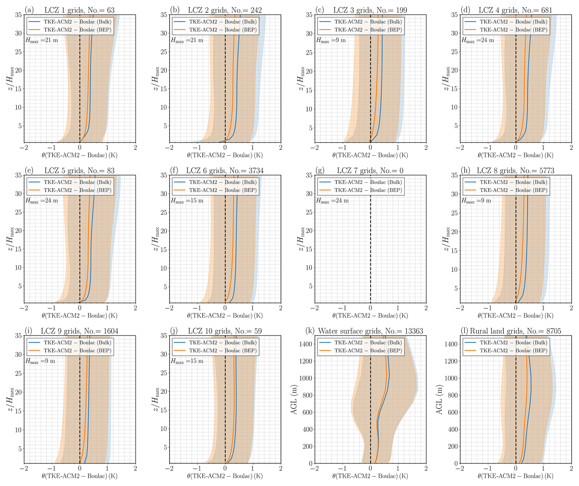
Figure 7 (a–j) Monthly mean vertical profiles of Δθ(TKE-ACM2−Boulac) with/without BEP over LCZ 1–10 (urban) grids; (k) over water surface girds; (l) over rural land cover grids. The blue and orange lines represent BEP and Bulk simulations, respectively. The shadowed area denotes ±1σ variability. The height is normalized relative to the maximum building height (H_max) for a specific urban LCZ type.

3.3 Case 24SC results: vertical profiles of $\mathit{\theta },u,\stackrel{\mathrm{‾}}{w^{\prime }{\mathit{\theta }}^{\prime }}$, and $\stackrel{\mathrm{‾}}{w^{\prime }{u}^{\prime }}$

The two PBL schemes performed similarly in Case 24SC, where TKE-ACM2+BEP simulated notably less warm bias in the UCL shown in Fig. 4c, particularly in the first model layer. In addition, the θ profile extending from the UCL up to 18H was considerably better reproduced by TKE-ACM2+BEP whereas Boulac+BEP simulated consistently cold bias below the inversion. There were similarities in the momentum profile between the 24SC and 10WC cases. First, Fig. 4d shows that Boulac+BEP predicted consistently lower wind speed than TKE-ACM2+BEP. Second, both BEP simulations tended to overestimate the wind speed in the UCL. Third, Bulk methods did not reproduce the inflection point and exhibited the greatest positive bias in the UCL. Finally, the wind shear at roof level had lower magnitudes in the two BEP simulations than in LES. The difference in performance was that TKE-ACM2+BEP had slightly less deviation from 1H to approximately 5H but made obvious overpredictions in [7H,17H]. In contrast, Boulac+BEP had a negative bias in [1H,7H] and provided a promising match in [7H,17H].

The heat flux profile for Case 24SC presented in Fig. 5c shows a visibly underestimated $\stackrel{\mathrm{‾}}{w^{\prime }{\mathit{\theta }}^{\prime }}$ in the mixed layer simulated by Boulac+BEP, which accounts for the cold bias. Conversely, the two Bulk simulations consistently had warm bias throughout the PBL, consistent with the trend in Case 10WC. Figure 5d indicates that TKE-ACM2+BEP yielded $\stackrel{\mathrm{‾}}{w^{\prime }{u}^{\prime }}$ with a similar pattern and magnitude to LES in the whole PBL, whereas Boulac+BEP seemed to largely underestimate the momentum flux as observed in the 10WC case. The two Bulk methods produced monotonically increasing momentum flux from the ground to the top of the boundary layer. The $\stackrel{\mathrm{‾}}{w^{\prime }{u}^{\prime }}$ in TKE-ACM2+Bulk was less negative than that in Boulac+Bulk (Fig. 5b and d), corroborating a relatively larger $u/u_{\mathrm{g}}$ (Fig. 4b and d) in both cases. In contrast, the momentum flux profiles simulated by BEP models had a local minimum value at or above the roof level. Below the roof level, TKE-ACM2+BEP yielded slightly more negative $\stackrel{\mathrm{‾}}{w^{\prime }{u}^{\prime }}$ than Boulac+BEP (Fig. 5b and d) consistently in the two cases, resulting in a lower wind speed (Fig. 4b and d). From the roof level to the top of the boundary layer, TKE-ACM2+BEP produced massively larger magnitudes of $\stackrel{\mathrm{‾}}{w^{\prime }{u}^{\prime }}$ due to the addition of the non-local flux, yet the $u/u_{\mathrm{g}}$ were lower in [18H,27H] ([16H,21H]) in Case 10WC (Case 24SC) only compared to Boulac+BEP, indicating an inconsistent correlation between $u/u_{\mathrm{g}}$ and $\stackrel{\mathrm{‾}}{w^{\prime }{u}^{\prime }}$ within Z=1H to Z=18H (Z=16H). This inconsistency is likely due to the fact that TKE-ACM2+BEP produced a more well-mixed boundary layer, resulting in $u/u_{\mathrm{g}}$ profiles within the mixed layer that exhibited less variability compared to those in Boulac+BEP, which appeared to have a stronger shear. There was a notable difference in $z/H_{{\stackrel{\mathrm{‾}}{w^{\prime }{u}^{\prime }}}_{\max }}$ between 24SC and 10WC; i.e., LES showed that $z/H_{{\stackrel{\mathrm{‾}}{w^{\prime }{u}^{\prime }}}_{\max }}$ increased from $z/H=\mathrm{1}$ to approximately $z/H=\mathrm{4}$ when ${\stackrel{\mathrm{‾}}{w^{\prime }{\mathit{\theta }}^{\prime }}}_{\mathrm{0}}$ was stronger. Further analysis involving the partitioning of total $\stackrel{\mathrm{‾}}{w^{\prime }{u}^{\prime }}$ revealed that the non-local component played a more important role in distributing the surface layer fluxes to the mixed layer in TKE-ACM2+BEP, as reflected by the blue dashed line in Fig. 5d. Compared with Case 10WC, the larger prescribed ${\stackrel{\mathrm{‾}}{w^{\prime }{\mathit{\theta }}^{\prime }}}_{\mathrm{0}}$ in Case 24SC suggested that TKE-ACM2+BEP achieved a closer match in the magnitude and shape of $\stackrel{\mathrm{‾}}{w^{\prime }{u}^{\prime }}$ at and immediately above roof level compared with Boulac+BEP. In addition, TKE-ACM2+BEP gave $z/H_{{\stackrel{\mathrm{‾}}{w^{\prime }{u}^{\prime }}}_{\max }}=\mathrm{3}$, which aligns more closely with LES results than Boulac+BEP ($z/H_{{\stackrel{\mathrm{‾}}{w^{\prime }{u}^{\prime }}}_{\max }}=\mathrm{1}$). Rotach (2001) analyzed several field measurements and wind tunnel experiments to examine the height of the maximum turbulence momentum flux. They found that $\stackrel{\mathrm{‾}}{w^{\prime }{u}^{\prime }}$ can occur at approximately 3H, which is deemed as the top of the RSL. This indicates that stronger heat flux can cause elevated $z/H_{{\stackrel{\mathrm{‾}}{w^{\prime }{u}^{\prime }}}_{\max }}$, requiring extra caution in the PBL scheme when dealing with a sizable urban morphology. In summary, the RMSE(u) was 0.33 m s⁻¹ for both TKE-ACM2+BEP and Boulac+BEP. This indicates that the two PBL schemes coupled with BEP performed similarly in simulating momentum profiles below the PBL height in Case 24SC and outperformed the Bulk methods. However, TKE-ACM2+BEP outperformed Boulac+BEP in Case 24SC in simulating the θ profile, reducing the RMSE by 75.6%, which aligns with its closer match of $\stackrel{\mathrm{‾}}{w^{\prime }{\mathit{\theta }}^{\prime }}$ in the mixed layer.

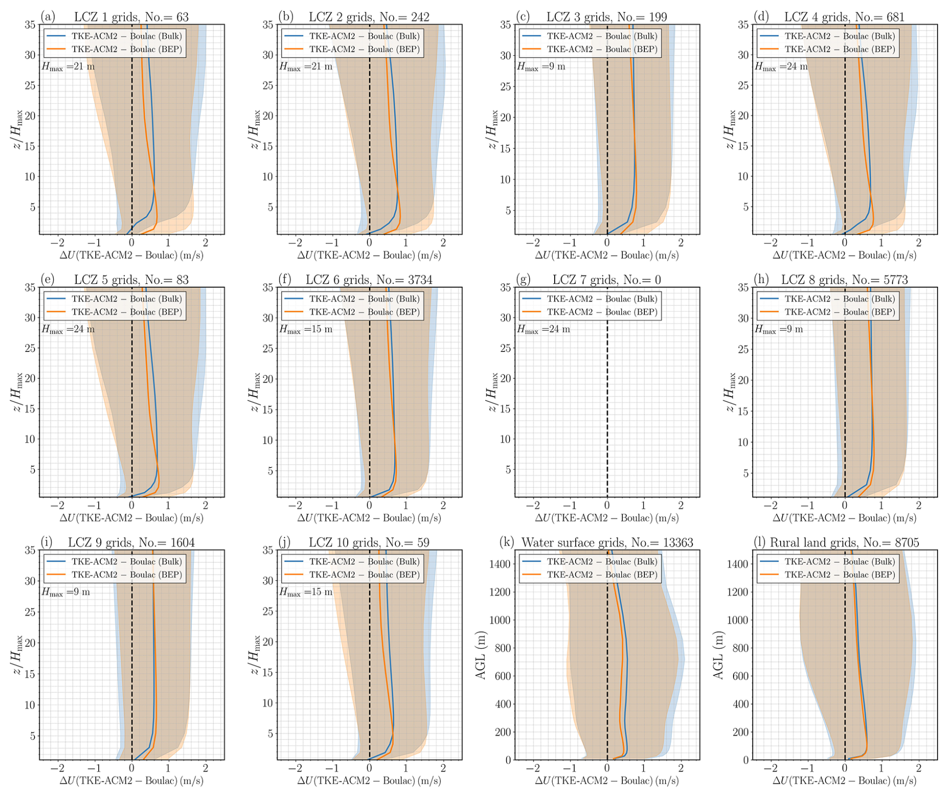
Figure 8 (a–j) Monthly mean vertical profiles of ΔU(TKE-ACM2−Boulac) with/without BEP over LCZ 1–10 (urban) grids; (k) over water surface girds; (l) over rural land cover grids. The blue and orange lines represent BEP and Bulk simulations, respectively. The shadowed area denotes ±1σ variability. The height is normalized relative to the maximum building height (H_max) for a specific urban LCZ type.

4 Real case simulation results

4.1 Impact of TKE-ACM2 on the vertical profiles of θ and U

Figures C1 and C2 (Appendix C) present the vertical profiles of θ and $U=\sqrt{u^{\mathrm{2}}+v^{\mathrm{2}}}$ averaged over the entire simulated month for ten LCZ urban classes, water surfaces, and rural land covers. Implementing the BEP scheme with both PBL schemes reduced θ and U by up to approximately 2 K and 2 m s⁻¹ respectively, below 35 times the maximum building height for each LCZ urban class (H_max), with the most pronounced differences occurring near the ground. Both BEP simulations had less pronounced differences in U over water surfaces and rural land cover compared with urban grids, primarily because the BEP model was not directly applied in these non-urban areas. Any observed differences in U in these regions resulted from the neighboring urban grids. The effects of BEP on U over urban grids align with simulations conducted for Berlin, Munich, and Prague (Karlický et al., 2018). Finally, complex interactions between the atmosphere and buildings, including radiative transfer (direct and reflected solar radiation and net longwave radiation), and thermal exchange between solid surfaces and the atmosphere, collectively led to the lower temperature in BEP simulations.

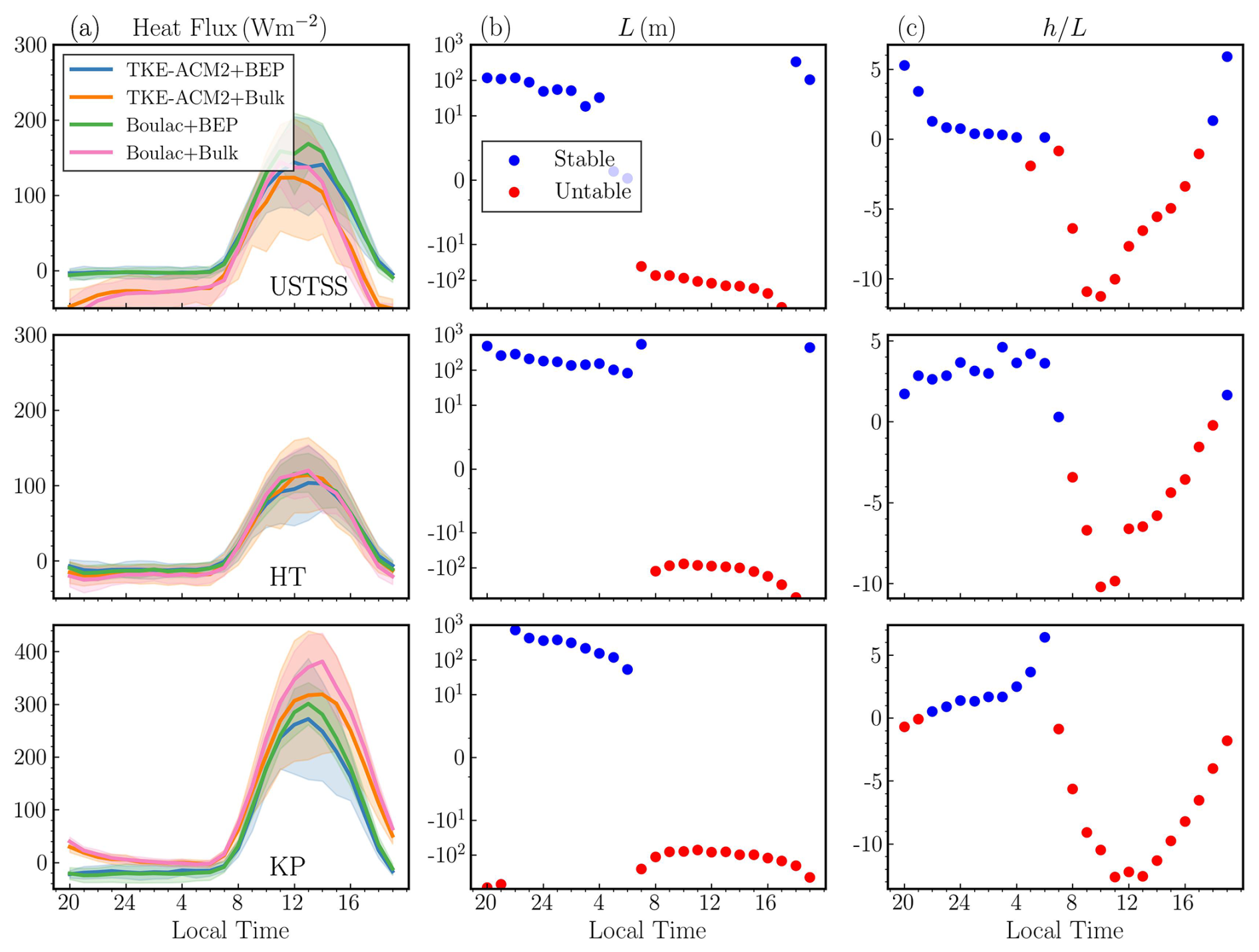
Figure 9 Column (a) monthly mean diurnal patterns of the surface heat flux for the grid point of the observation sites (Fig. 2) USTSS_LCZ5, HT_rural, and KP_LCZ1 from top to bottom; Column (b) Obukhov length (L) with a semi-log y-axis; Column (c) stability parameter ($h/L$). The integration is from 20:00 UTC+8 on 18 July in 2022 to 20:00 UTC+8 on 18 August in 2022.

The influence of the TKE-ACM2 PBL scheme was assessed by comparing θ and U profiles with those from Boulac, both with and without BEP, as shown in Figs. 7 and 8. TKE-ACM2 generally predicted a warmer θ than Boulac across urban, water, and rural grids, regardless of BEP activation. However, the difference Δθ(TKE-ACM2−Boulac), was slightly less in the BEP simulations than in Bulk simulations across all grids.

Moreover, TKE-ACM2 consistently simulated higher wind speeds above the canopy height than Boulac, particularly when paired with BEP, aligning with results from idealized simulations (Fig. 4b and d). There were instances where the average ΔU(TKE-ACM2−Boulac) was negative at the first model height (9 to 10 m) for the Bulk method, notably at LCZ 1, 2, 4, and 10. Nonetheless, in BEP simulations, ΔU(TKE-ACM2−Boulac) was a maximum over urban grids at approximately 2 to 4 times H_max, compared with approximately about 5 times H_max in Bulk simulations.

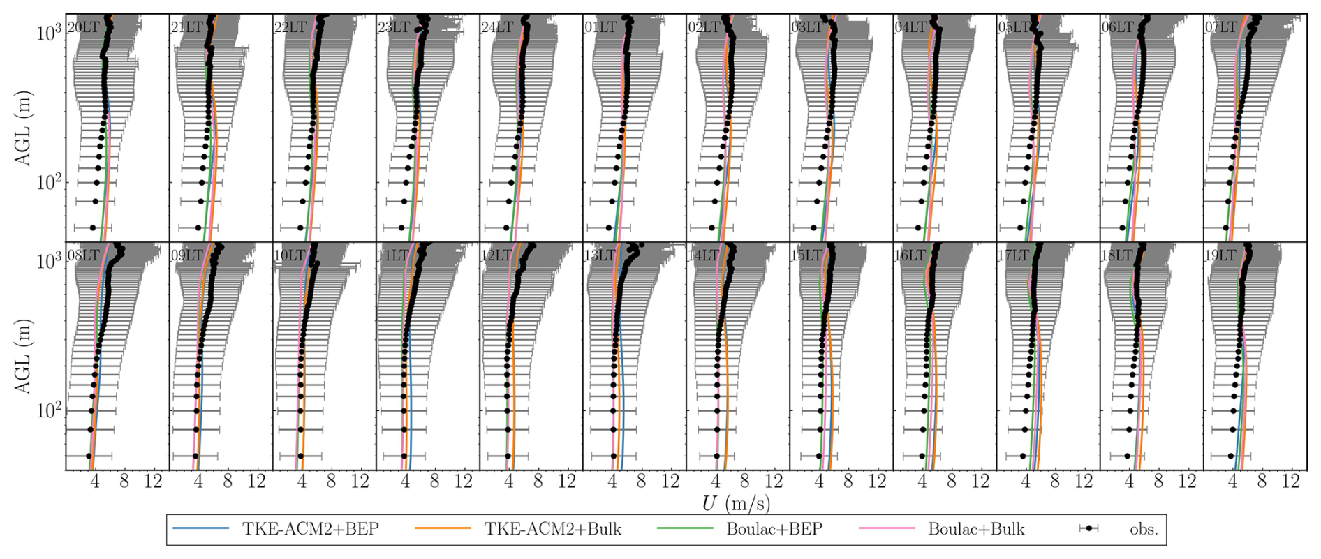
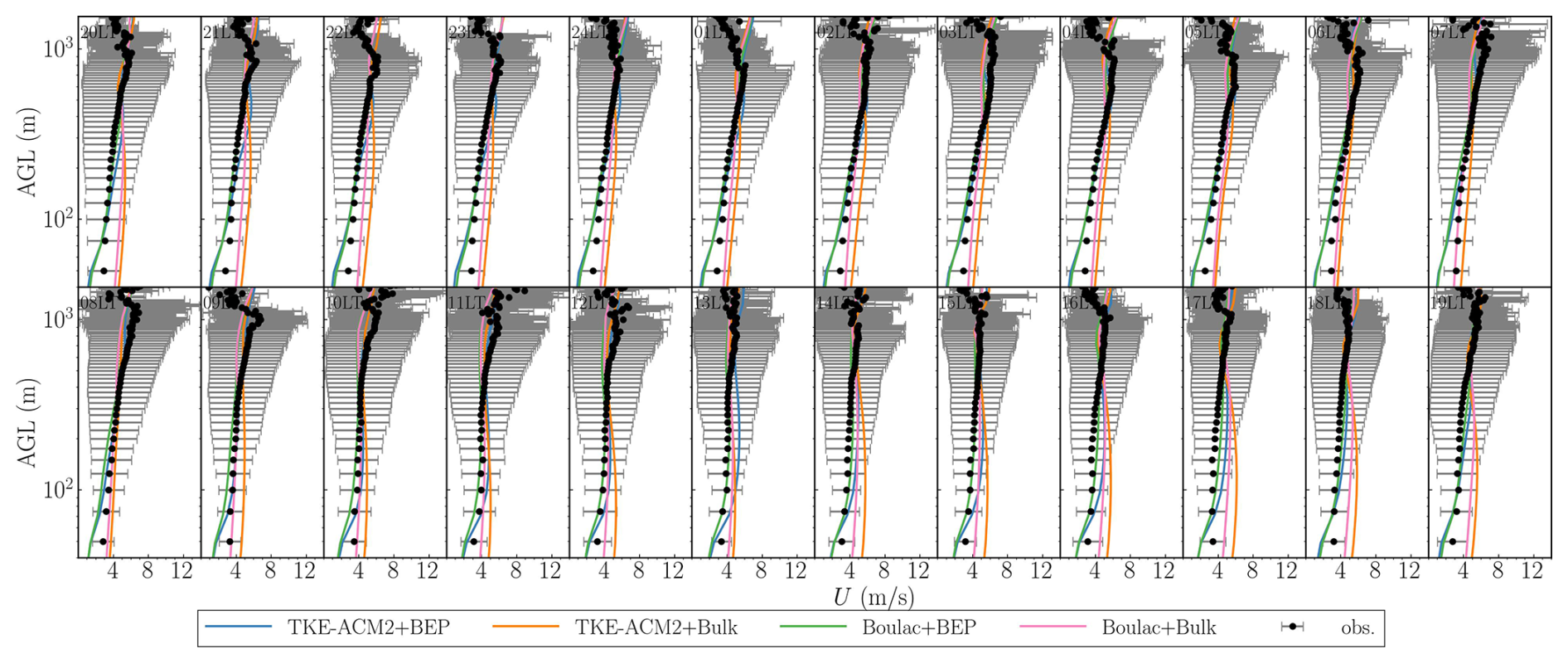
Figure 10 Monthly mean vertical profiles of wind speeds at the USTSS_LCZ5 LiDAR station. The blue, orange, green, and pink lines denote the results of TKE-ACM2+BEP, TKE-ACM2+Bulk, Boulac+BEP, and Boulac+Bulk, respectively. The black dots represent the LiDAR measurements, with the error bar indicating the ±1 standard deviation. The integration is from 20:00 UTC+8 on 18 July in 2022 to 20:00 UTC+8 on 18 August in 2022.

Figure 11 Same as Fig. 10 but for the HT_rural LiDAR station.

Figure 12 Same as Fig. 10 but for the KP_LCZ1 LiDAR station.

4.2 Monthly mean diurnal profiles of U compared with high-resolution LiDAR measurements

The monthly mean diurnal variations of the heat flux, Obukhov length (L), and stability parameter ($h/L$) are presented in Fig. 9. At the HT_rural LiDAR station, the heat flux pattern did not exhibit a notable difference. However, the USTSS_LCZ5 LiDAR location, introducing BEP consistently resulted in a greater surface heat flux compared with the Bulk methods. In contrast, at KP_LCZ1, BEP simulations produced a lower surface heat flux throughout the diurnal cycle.

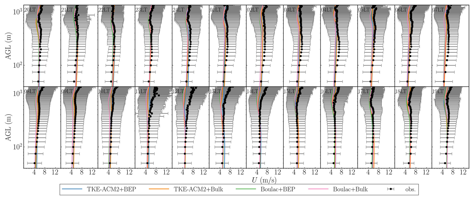
The wind speed LiDAR offers hourly measurements of wind speed at an altitude of 50 m a.g.l., with vertical increments of 25 m. The measured and simulated wind speed profiles averaged across the whole month are presented for each hour in Fig. 10 (USTSS_LCZ5), Fig. 11 (HT_rural), and Fig. 12 (KP_LCZ1). To quantify the performance of each simulation, the RMSE and mean bias (MB) between the simulated profiles and LiDAR measurements are presented in Fig. 13.

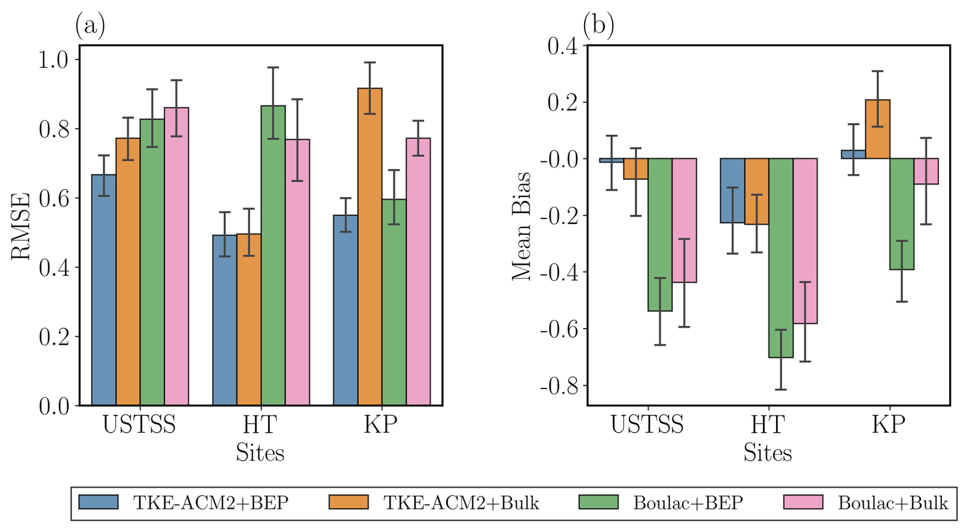
Figure 13 RMSE (a) and MB (b) of the monthly averaged diurnal variation of vertical profiles of wind speeds calculated at the three LiDAR stations for four simulations obtained by taking LiDAR measurements as the reference. The error bars represent the ±1σ variability of the RMSE/Mean bias of a diurnal cycle.

Although USTSS_LCZ5 was located in a model grid classified as open mid-rise, applying BEP did not consistently result in a notable reduction in wind speed. This contrasts with the average decrease of ∼1–2 m s⁻¹ observed across all LCZ 5 grids, as shown in Fig. C2e. A possible explanation is that the LCZ map in Fig. 2b indicates that the model grid containing USTSS_LCZ5 was bordered by either rural land or water grids, effectively isolating it from other urban grids. Consequently, the wind approaching this grid experienced a less rough fetch, leading to a reduced drag exerted on this model grid. The overprediction occurred primarily below ∼300 m during the night for all schemes, with BEP simulations producing a slightly smaller positive bias. The overestimation below ∼300 m persisted in TKE-ACM2+BEP from 11:00 local time (LT) to 17:00 LT, whereas Boulac+BEP aligned better with observations. Furthermore, all schemes exhibited underestimation above ∼300 m. Consistent with the accelerated wind speed shown in Fig. C2, TKE-ACM2+BEP produced slightly larger U beyond ∼300 m, leading to the smallest positive bias relative to the LiDAR observations. The accelerated U observed in the upper PBL was also evident in the 10WC and 24SC idealized cases (Fig. 4b and d). Finally, detailed analysis reveals that the wind speed profiles during the night showed less difference between schemes compared with U simulated during the day. This is probably because TKE-ACM2 and Boulac adopt similar turbulence closure models; their performance may differ less when there is an absence of convective thermals. In summary, the histograms in Fig. 13 show that TKE-ACM2+BEP yielded the smallest RMSE and the smallest negative MB, whereas Boulac+BEP led to greater deviations compared with Boulac+Bulk.

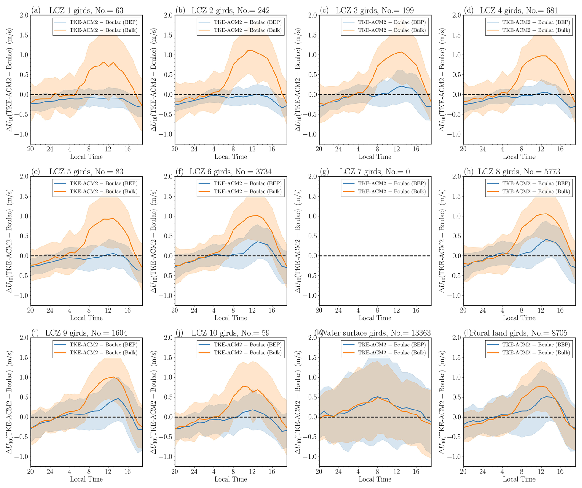
Figure 14 (a–j) Monthly mean ΔU₁₀(TKE-ACM2−Boulac) over LCZ 1–10 (urban) grids; (k) over water surface grids; (l) over rural land cover grids. The blue and orange lines represent the results of BEP and Bulk simulations, respectively. The shadowed area indicates ±1σ variability.

Figure 15 Same as Fig. 14 but for T₂.

Figure 16 Same as Fig. 14 but for RH₂.

At the rural LiDAR station HT_rural, the application of BEP had a limited impact on the PBL performance over non-urban model grids, supporting the conclusion drawn in Sect. 4.1. The differences between BEP and Bulk were indistinguishable below ∼400 m. However, TKE-ACM2+BEP occasionally accelerated U beyond ∼600 m, such as from 10:00 to 13:00 LT, aligning more closely with LiDAR observations. Overall, BEP introduced only minor variations in U profiles within non-urban model grids, particularly in the lower PBL. Therefore, the differences in the accuracy of U within this height range over non-urban grids were largely caused by the PBL schemes rather than the UCMs. Nonetheless, BEP had a slightly more pronounced effect in TKE-ACM2+BEP by accelerating U in the upper PBL, leading to the improved reproduction of U profiles at HT_rural LiDAR station. In contrast with the USTSS_LCZ5 station, which was located in an isolated LCZ 5 grid, the KP_LCZ1 station was situated in the densely developed downtown area of Hong Kong, surrounded by an extensively built-up environment. Both schemes coupled with BEP exhibited considerably decelerated wind speeds below ∼400 m, corroborating the trend observed for all LCZ 1 girds shown in Fig. C2a. Notably, discrepancies were reduced within 100–400 m range, where wind speeds tended to be overestimated. However, BEP tended to excessively reduce wind speeds in both schemes from 50 to 100 m, approximately 2.5 to 5 times H_max for this LCZ type, particularly closer to ground level. In contrast, the Bulk methods produced bias of similar magnitudes but with a reverse sign below 100 m. In the 600–1000 m range, Boulac+BEP gave the lowest wind speeds during the day and yielded wind speeds comparable to those of TKE-ACM2+BEP at night. Moreover, the performance of TKE-ACM2+BEP differed from that of Boulac+BEP in the 600–1000 m range in that it generated a less negatively biased wind speed at particular hours, such as from 08:00 to 12:00 LT. Overall, the two PBL schemes coupled with BEP had a considerably better RMSE than the Bulk methods at this particular compact high-rise grid. More specifically, TKE-ACM2+BEP outperformed TKE-ACM2+Bulk, reducing the RMSE from 0.92 to 0.55 m s⁻¹ and reducing the MB from 0.21 to 0.03 m s⁻¹. In addition, TKE-ACM2+BEP performed slightly better than Boulac+BEP, which had an RMSE of 0.60 m s⁻¹.

4.3 Impact of TKE-ACM2 on U₁₀, T₂, and RH₂

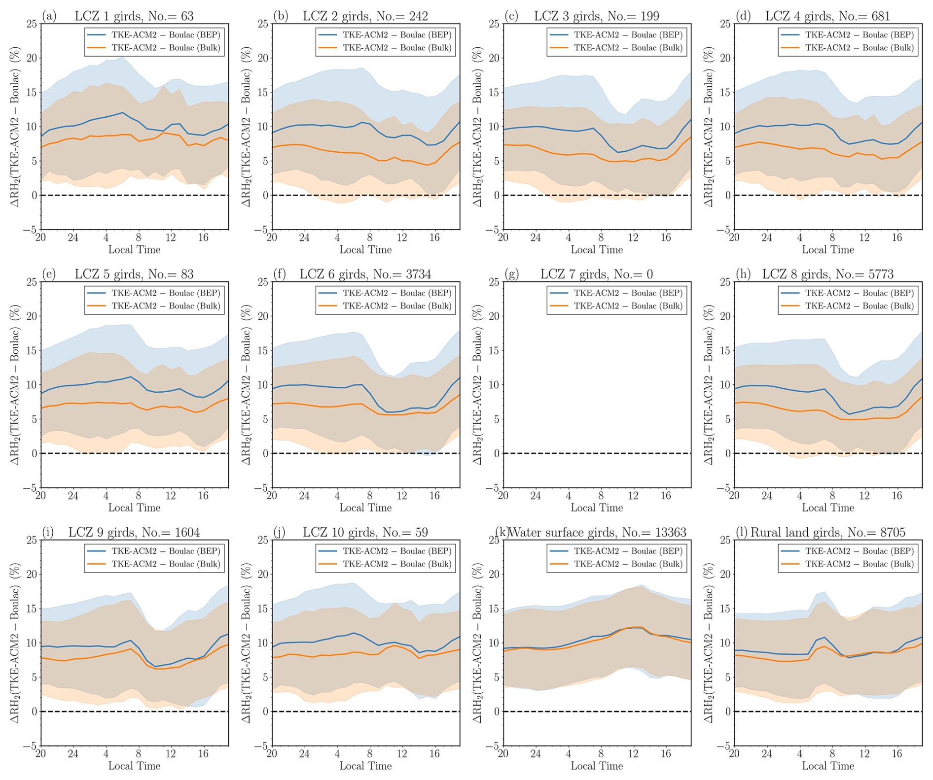
Figures C3, C4, and C5 (Appendix C) present the diurnal patterns of U₁₀, T₂, and 2 m relative humidity (RH2) simulated using the four configurations. The impact of TKE-ACM2 on these surface meteorological variables, relative to Boulac, was examined in simulations with and without BEP, as shown in Figs. 14 (U₁₀), 15 (T₂), and 16 (RH₂).

Notably, the difference in U₁₀ between TKE-ACM2 and Boulac was greatest at 12:00 LT, aligning with the peak sensible heat flux (Fig. 9a). This deviation arose because TKE-ACM2 incorporated non-local momentum transport that scaled with atmospheric instability, whereas Boulac adopted fully local momentum transport. However, incorporating BEP reduced this difference in urban grids, as BEP effectively lowered U₁₀ (Fig. C3). Specifically, TKE-ACM2+Bulk produced higher wind speeds than Boulac+Bulk during the day by up to 1 m s⁻¹, a difference that diminished to less than 0.4 m s⁻¹ with BEP integration.

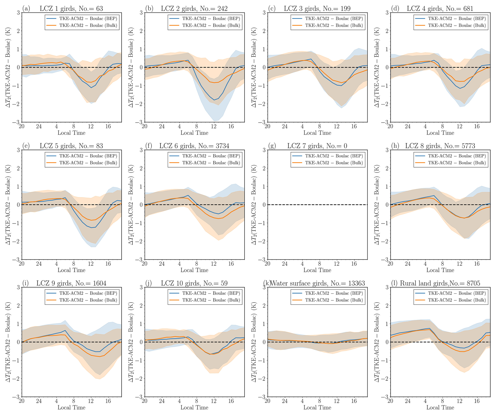
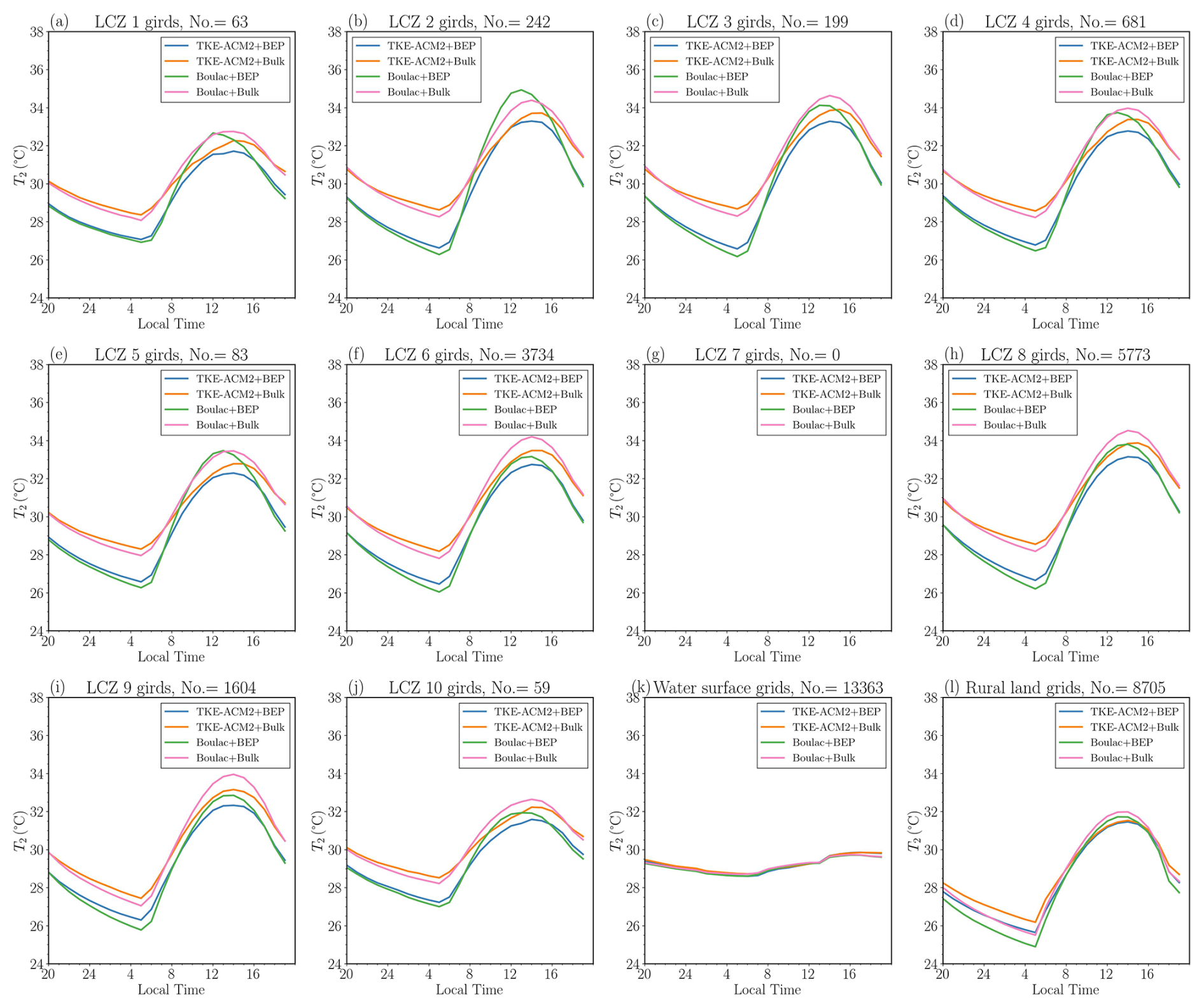
Figure 15 shows that the temperature difference ΔT₂(TKE-ACM2−Boulac) followed a diurnal pattern, with TKE-ACM2 consistently simulating lower T₂ at 12:00 LT relative to Boulac which aligns with the results of idealized simulations with a similar heat flux magnitude (Case 24SC depicted in Fig. 4c). Importantly, with BEP, this temperature difference increased at noon, particularly across LCZ 1 to 5 grids. In contrast, ΔRH₂ remained positively biased and further increased when BEP was applied.

4.4 Monthly mean diurnal patterns of U₁₀, T₂, and RH₂ compared with surface stations

Time series data for each station are provided in the Supplement of Zhang (2024) for detailed visualization. The diurnal variations of U₁₀, T₂, and RH₂ for a total of 31 surface stations were aggregated based on their LCZ classifications, as shown in Figs. 17, 18, and 19, respectively. RMSE histograms are presented in Fig. 20. The adoption of BEP reduced U₁₀, which aligns with the trend observed in Fig. C3 for all LCZ urban grids. This reduction greatly improved the reproduction of U₁₀ at LCZ 5, 6, and 8 stations, which were primarily in areas with low- or mid-rise buildings at relatively low building density. Closer inspection reveals that the improvements were more profound at night over the aforementioned stations. Among these stations, TKE-ACM2+BEP performed the best or comparably to Boulac+BEP with an RMSE as small as 1.0 m s⁻¹. However, the wind speeds simulated using BEP at LCZ 1, 2, 4, and 10 stations were considerably smaller than observed values, particularly during the day. The large underestimation of U₁₀ at the LCZ 1 surface station aligns with the underestimation of U at 50 m at the KP_LCZ1 LiDAR station. Specifically, both BEP simulations consistently produced U₁₀≈1 m s⁻¹ with an RMSE 1.7–2.4 m s⁻¹, which was worse than the RMSE of Bulk methods (RMSE ∼1.5 m s⁻¹). The excessive reduction in U₁₀ is likely to be due to the mismatch between local LCZ classification (100 m resolution) and re-gridded LCZ classification (1 km resolution) at LCZ 1, 4, and 10 stations, reported by Ribeiro et al. (2021). For instance, the surface station co-located with the KP_LCZ1 LiDAR, also classified as an LCZ 1 station, was situated on a hill with a spatial scale of 50 m. Therefore, the immediate surroundings of the KP surface station were relatively open and flat. Nonetheless, another source of discrepancy stemmed from the use of a look-up table to determine urban canopy parameters (UCPs). This approach overlooks the heterogeneity of UCPs within a given LCZ urban class, leading to results that are less accurate than those of a gridded UCP method (Sun et al., 2021). As highlighted by Shen et al. (2019), among the critical UCP factors, the urban fraction is important in simulating horizontal wind speeds. However, the current study did not account for the variability of the urban fraction or the distribution of building heights within specified LCZ urban classes. As a result, the model underestimated U₁₀, suggesting potentially poor representativeness at the station's exact location.

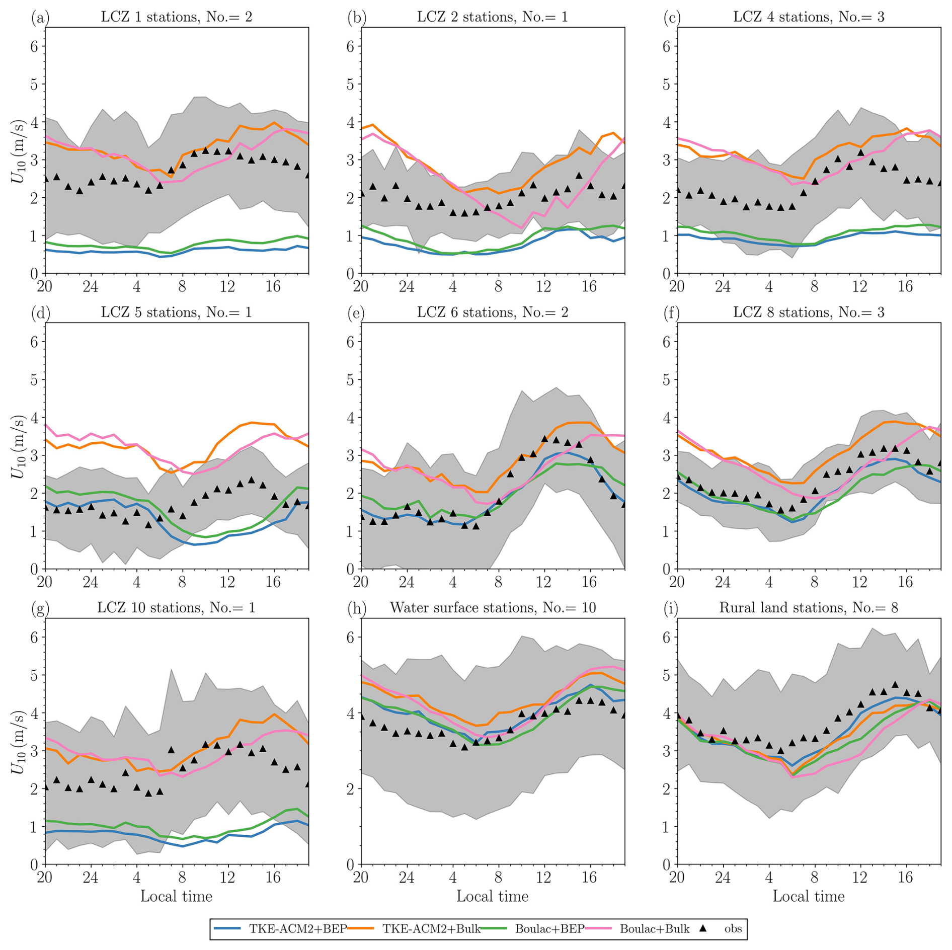
Figure 17 Comparison of monthly mean diurnal patterns of U₁₀ with observations made at surface stations. The title of each panel describes the LCZ type and the number of associated surface stations. The blue, orange, green, and pink lines represent results of the TKE-ACM2+BEP, TKE-ACM+Bulk, Boulac+BEP, and Boulac+Bulk, respectively. The black markers indicate the surface station observations. The gray shadowed area indicates the ±1σ variability of observations.

Figure 18 Same as Fig. 17 but for T₂ comparison.

Figure 19 Same as Fig. 17 but for RH₂ comparison.

Figure 20 RMSE for aggregated station types, with (a), (b), and (c) representing U₁₀, T₂, and RH₂, respectively. The number of stations contributing to an LCZ type is given in the sub-titles in Figs. 17, 18, or 19.

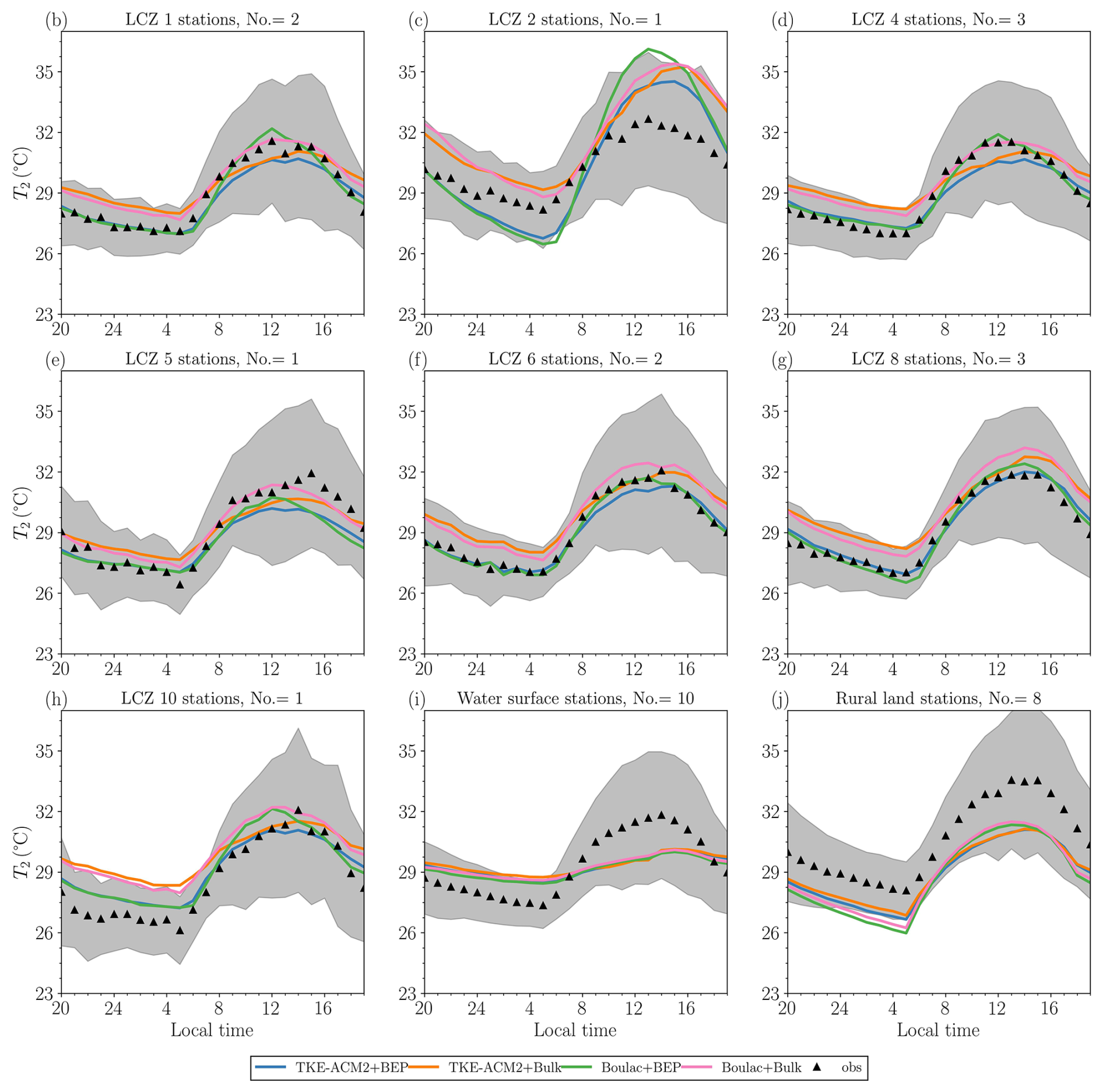
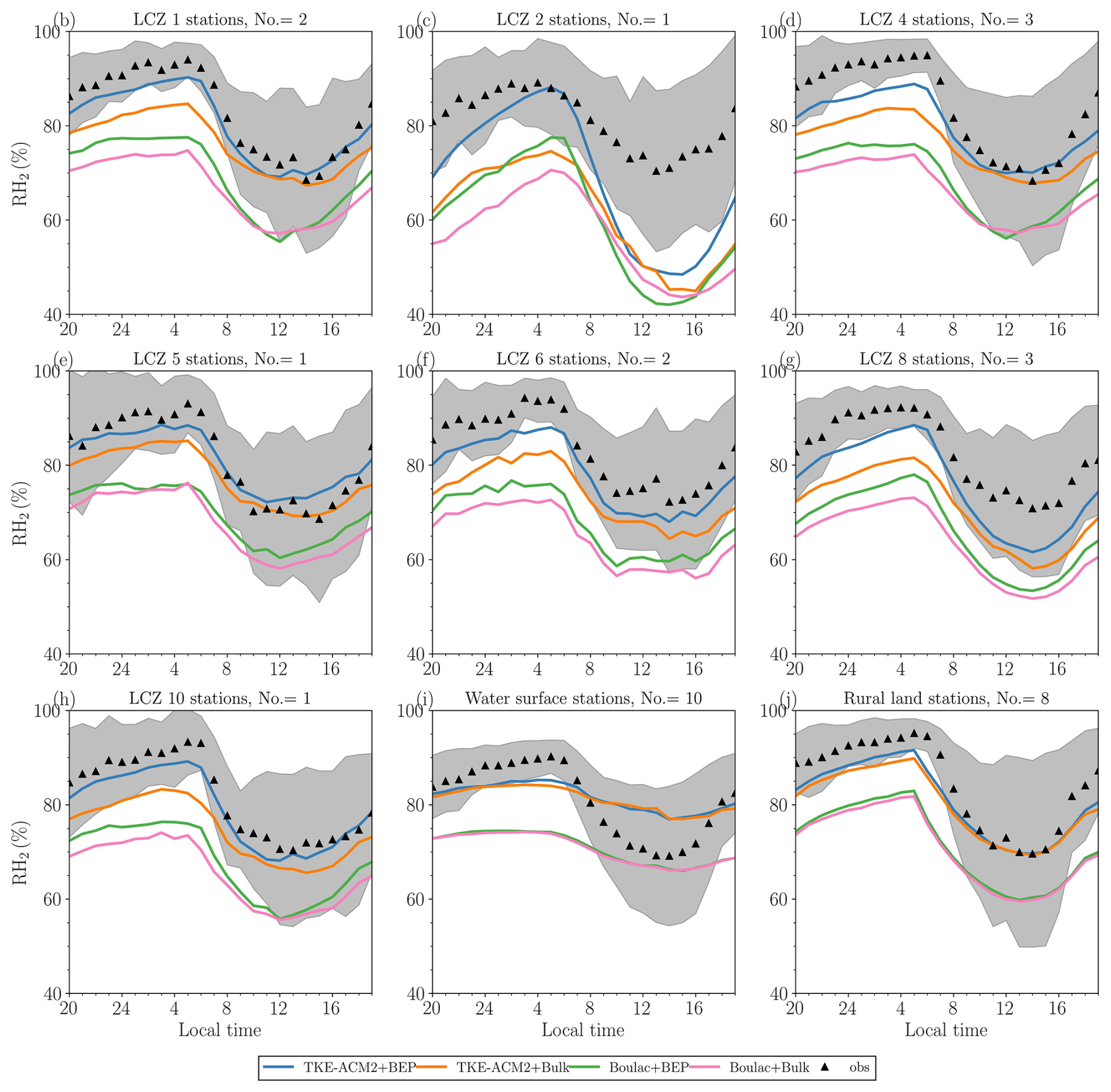
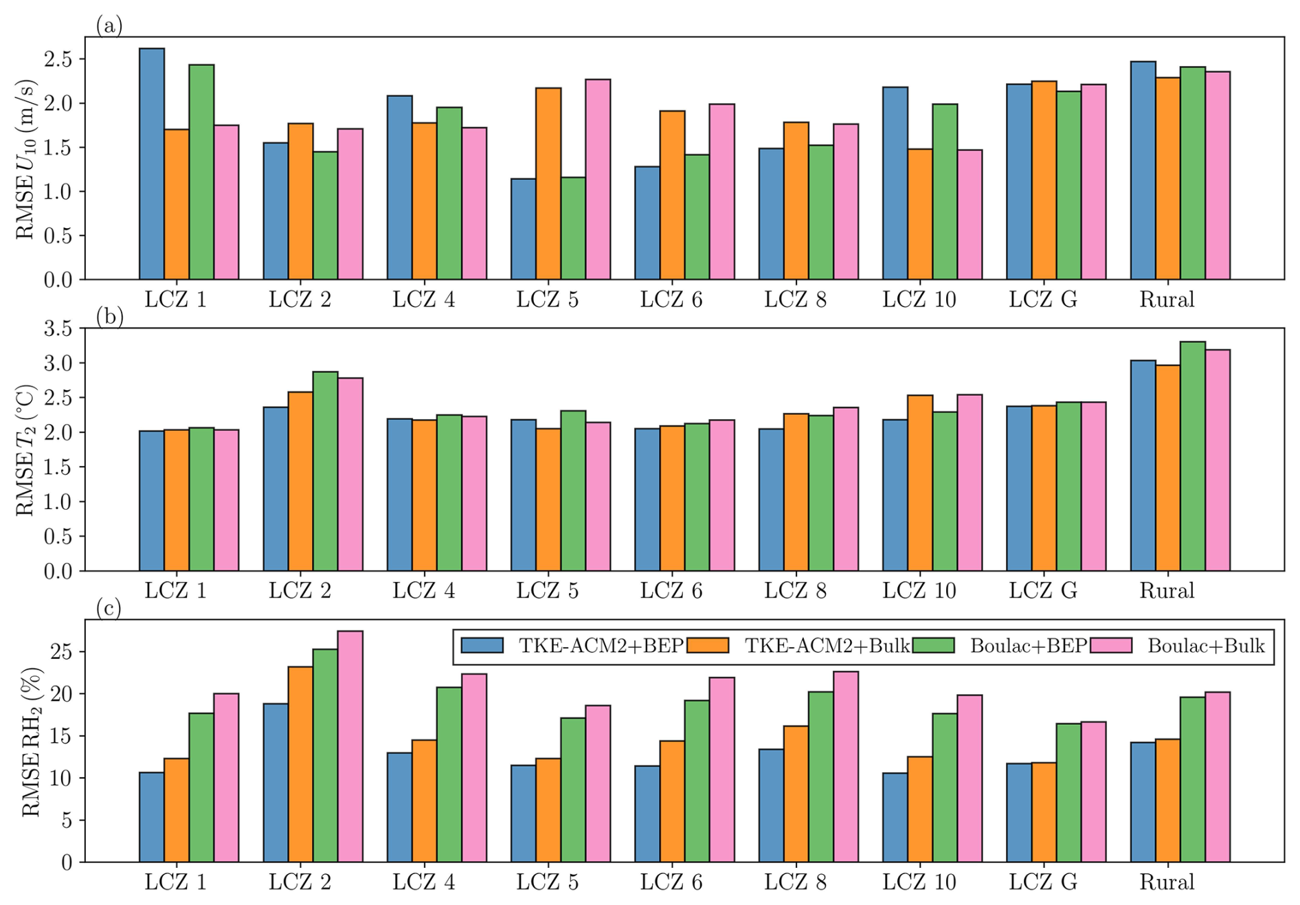
Figure C4 shows that T₂ at night was reduced in BEP simulations over all LCZ urban stations. The change in T₂ was smaller during the day, and Boulac+BEP was likely to produce a warmer daytime T₂ than TKE-ACM2+BEP. As a result, the coupling of either PBL scheme with BEP considerably improved the warm bias at night relative to Bulk methods, and their accuracy during the day hardly changed. TKE-ACM2+BEP outperformed Boulac+BEP over LCZ 2, 5, 8, and 10 stations, with the RMSE(T₂) reduced by 0.51, 0.13, 0.27, and 0.11 K, respectively. The performance in the two simulations was comparable for other LCZ urban stations. The four simulations generated T₂ diurnal cycles with much lower amplitude than observations at water surfaces, where the inter-scheme difference was marginal and each scheme deviated from observations by ∼2 K. The significantly smaller diurnal cycle produced by the simulations compared to observations can be attributed to several stations located on small islands or along the coast. In these cases, the model identified the grid point as the water surface which occupied a greater fraction than land. At rural land stations, T₂ was consistently underestimated across all simulations. This underestimation was slightly exacerbated at night in BEP simulations, probably due to the effects of adjacent urban grids.

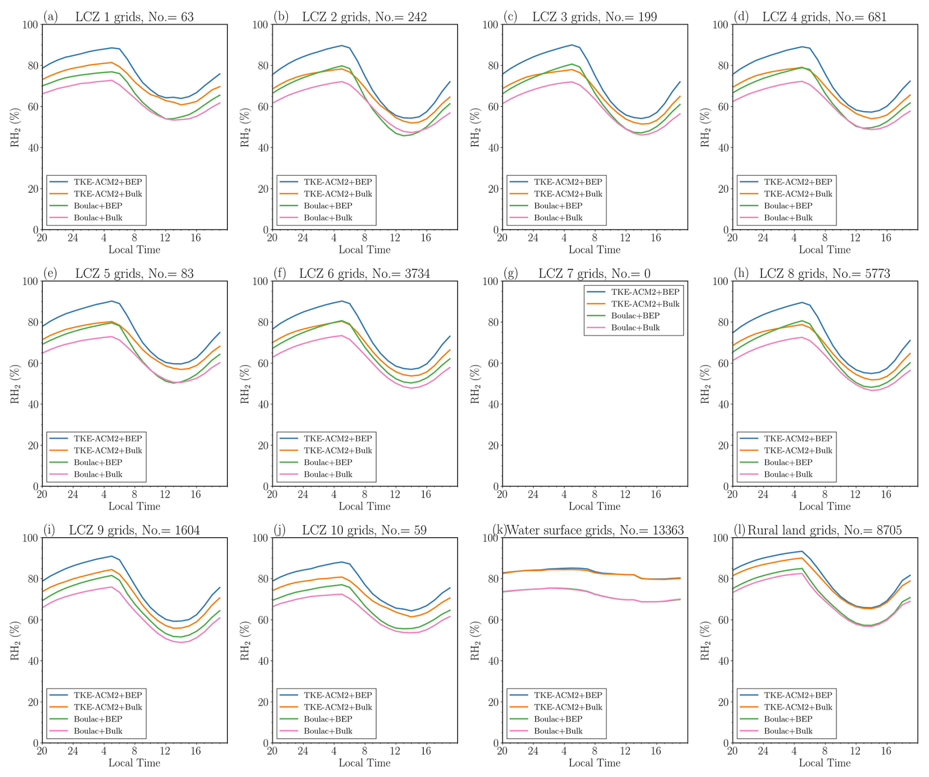
Lastly, Boulac generated a much dryer boundary layer than observations for all types of surface stations, regardless of the choice of surface layer flux parameterizations. Similar to Boulac+Bulk, TKE-ACM2+Bulk produced a dryer surface layer but with much less negative bias. The addition of BEP to the two PBL schemes greatly improved the accuracy of RH₂ at urban stations by simulating moister air. Figure C5 shows that BEP produced an increasingly large RH₂ when coupled with TKE-ACM2 rather than with Boulac, resulting in a more profound improvement in TKE-ACM2+BEP. In summary, BEP affected not only the surface wind speed but the T₂ and RH₂ diurnal patterns. TKE-ACM2+BEP outperformed other schemes in terms of reducing warm bias at night and enhancing the accuracy in simulating RH₂ at urban stations.

5 Conclusions

In this study, we developed a numerical method for coupling BEP with the TKE-ACM2 planetary boundary layer scheme detailed by Zhang et al. (2024). We first evaluated the performance of TKE-ACM2+BEP under a series of idealized atmospheric conditions with a simplified urban morphology in the WRF model. We used a state-of-the-art large-eddy simulation tool, PALM, configured with three-dimensional equidistant resolution, to provide a reference result at the building-resolving scale. We demonstrated that TKE-ACM2+BEP outperformed TKE-ACM2 without an urban canopy model in reproducing the vertical profiles of θ and u in two prescribed surface heat flux cases. Moreover, TKE-ACM2+BEP outperformed the widely used Boulac+BEP scheme in the moderately convective case. In particular, TKE-ACM2+BEP predicted θ with a reduced warm bias within the urban canopy layer. In addition, Boulac+BEP produced a sharper $\partial \mathit{\theta }/\partial z$ at the roof level, leading to a notable cold bias in the mixed layer. Closer inspection suggested that turbulent fluxes were better reproduced by TKE-ACM2+BEP, which is attributable to non-local fluxes. In contrast, Boulac+BEP underestimated their magnitudes.

Real case simulations adopting different parameterization schemes for surface layer fluxes were performed. TKE-ACM2+BEP behaved similarly to Boulac+BEP, with both reducing U below a certain height over the LCZ urban grids relative to Bulk simulations. Likewise, the effects of BEP considering the radiative transfer and sensible heat fluxes between solid surfaces and the atmosphere ultimately led to a lower θ over all urban grids. High-resolution wind speed LiDAR observations were used to evaluate the performance of TKE-ACM2+BEP. The reduction in U at USTSS_LCZ5 was not consistently observed across a diurnal cycle, which is probably attributable to the fact that USTSS_LCZ5 was located in an isolated urban grid with a smoother fetch in all directions. BEP hardly affected the wind speed profiles at the HT_rural station, where the four simulations performed similarly. Finally, TKE-ACM2+BEP outperformed TKE-ACM2+Bulk in reproducing vertical profiles of U at the LCZ 1 LiDAR station. In particular, the overestimation in the lower boundary layer was much improved. However, the wind speeds were overly reduced by BEP in Boulac and TKE-ACM2 below ∼100 m. Overall, TKE-ACM2+BEP outperformed other schemes in simulating the wind speed profile at this highly urbanized LiDAR station.

BEP did not necessarily improve the prediction of U₁₀ at all types of urban stations as it could lead to largely underestimated U₁₀ relative to the two schemes with Bulk methods. For instance, extremely low wind speeds were observed at LCZ 1, 2, 4, and 10 stations, which were in areas that had mostly compact or high-rise buildings. The enhanced accuracy of U₁₀ simulated by TKE-ACM2+BEP was notable at stations located in areas of relatively low building density, such as LCZ 5, 6, and 8 stations. The non-linear feedback to U₁₀ at rural stations was slightly improved by TKE-ACM2+BEP, with the RMSE reducing by ∼0.2 m s⁻¹. It is thus critical to select an appropriate configuration for simulating the wind speed throughout the boundary layer. Nonetheless, BEP consistently improved the reproduction of T₂ for TKE-ACM2 over urban stations, particularly reducing warm bias at night. T₂ simulated by TKE-ACM2+BEP was generally comparable to or slightly better than that simulated by Boulac+BEP at most urban stations. Moreover, the sensitivity of RH₂ to PBL scheme was comparable to that of UCMs. BEP led to moister PBL, and TKE-ACM2+BEP exhibited the least dry bias in reproducing RH₂ among all simulations. The present work did not aim to demonstrate that the new TKE-ACM2+BEP performs definitively better than other combinations of PBL and UCM in simulating all aspects of meteorological variables; rather, it offers valuable insights for selecting appropriate model configurations to meet various objectives regarding different atmospheric processes.

Appendix A: Numerical solutions to Eq. (3)

Equation (3) can be solved by re-writing it as the linear system Ax=b, where the column vector x contains the unknown prognostic variable ${\mathit{\zeta }}_i^{n+\mathrm{1}}$, the square boarded band matrix A is the coefficient matrix, which comprises the first column entry (E), diagonal (D), upper diagonal (U), and lower diagonal (L) elements, and the column vector b comprises the explicit terms used in Eq. (3). To keep the same order of numerical accuracy as TKE-ACM2 (Zhang et al., 2024), the Crank-Nicolson scheme is retained. This splits ${\mathit{\zeta }}_i^{n+\mathrm{1}}$ to $C{\mathit{\zeta }}_i^{n+\mathrm{1}}+(\mathrm{1}-C){\mathit{\zeta }}_i^n$ with C=0.5 being the Crank-Nicolson factor. Subsequently, the element in the ith row and ith column of D is expressed as

$$\begin{array}{}\text{(A1)}& \begin{array}{rl}{\mathbf{\text{D}}}_{i,i}& =\mathrm{1}+C{f}_{\text{conv }}{\mathrm{Md}}_i\mathrm{\Delta }t\\ & +C\left(\mathrm{1}-f_{\mathrm{conv}}\right){\displaystyle \frac{\mathrm{\Delta }t}{\mathrm{\Delta }{z}_i}}\left({\displaystyle \frac{K_I{S}_I}{\mathrm{\Delta }{z}_I}}+{\displaystyle \frac{K_{I-\mathrm{1}}{S}_{I-\mathrm{1}}}{\mathrm{\Delta }{z}_{I-\mathrm{1}}}}\right)-C{A}_i\mathrm{\Delta }t\end{array}\end{array}$$

The ith row element of column vector b is expressed as:

$$\begin{array}{}\text{(A2)}& \begin{array}{rl}{\mathit{b}}_i& ={\mathit{\zeta }}_i^n+(\mathrm{1}-C)f_{\text{conv }}\mathrm{Mu}{\mathit{\zeta }}_{\mathrm{1}}^n\mathrm{\Delta }t\\ & -(\mathrm{1}-C)f_{\text{conv }}{\mathit{\zeta }}_i^n\mathrm{\Delta }t+(\mathrm{1}-C)f_{\text{conv }}{\mathrm{Md}}_{i+\mathrm{1}}{\mathit{\zeta }}_I^n{\displaystyle \frac{\mathrm{\Delta }{z}_{i+\mathrm{1}}}{\mathrm{\Delta }{z}_i}}\mathrm{\Delta }t\\ & +{\displaystyle \frac{\mathrm{1}-C}{V_i\mathrm{\Delta }{z}_i}}{f}_{\text{conv }}(K_I{S}_I{\displaystyle \frac{{\mathit{\zeta }}_{i+\mathrm{1}}^n-{\mathit{\zeta }}_i^n}{\mathrm{\Delta }{z}_I}}\\ & -K_{I-\mathrm{1}}{S}_{I-\mathrm{1}}{\displaystyle \frac{{\mathit{\zeta }}_i^n-{\mathit{\zeta }}_{i-\mathrm{1}}^n}{\mathrm{\Delta }{z}_{I-\mathrm{1}}}})\mathrm{\Delta }t\\ & +(\mathrm{1}-C)A_i{\mathit{\zeta }}_i^n\mathrm{\Delta }t+B_i\mathrm{\Delta }t\end{array}\end{array}$$

The elements in the ith row and jth column of U, L, and E, are the same as those in Eqs. (13), (14), and (15) in Zhang et al. (2024), respectively, except that an additional multiple of $S_I/V_i$ applies to K_I.

Appendix B: LCZ classification and namelist configuration in WRF real case simulations

Table B1 Local Climate Zones (LCZ) classification scheme.

(Hong et al., 2004)(Iacono et al., 2008)(Iacono et al., 2008)(Jiménez et al., 2012)(Chen and Dudhia, 2001)(Gall et al., 2013)

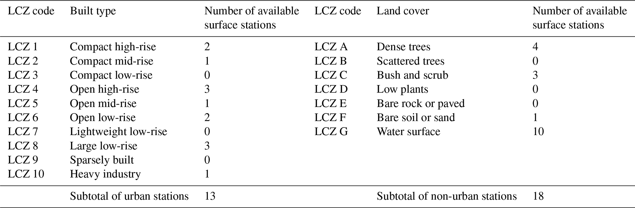
Table B2 Configurations of WRF version 4.3.3 settings for simulations using Boulac and TKE-ACM2 PBL schemes and UCM schemes.

Appendix C: θ and U profiles aggregated at different landuse

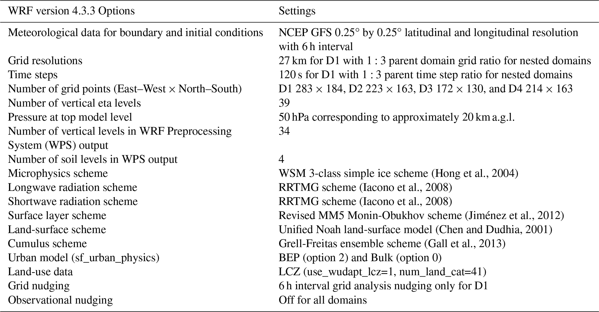
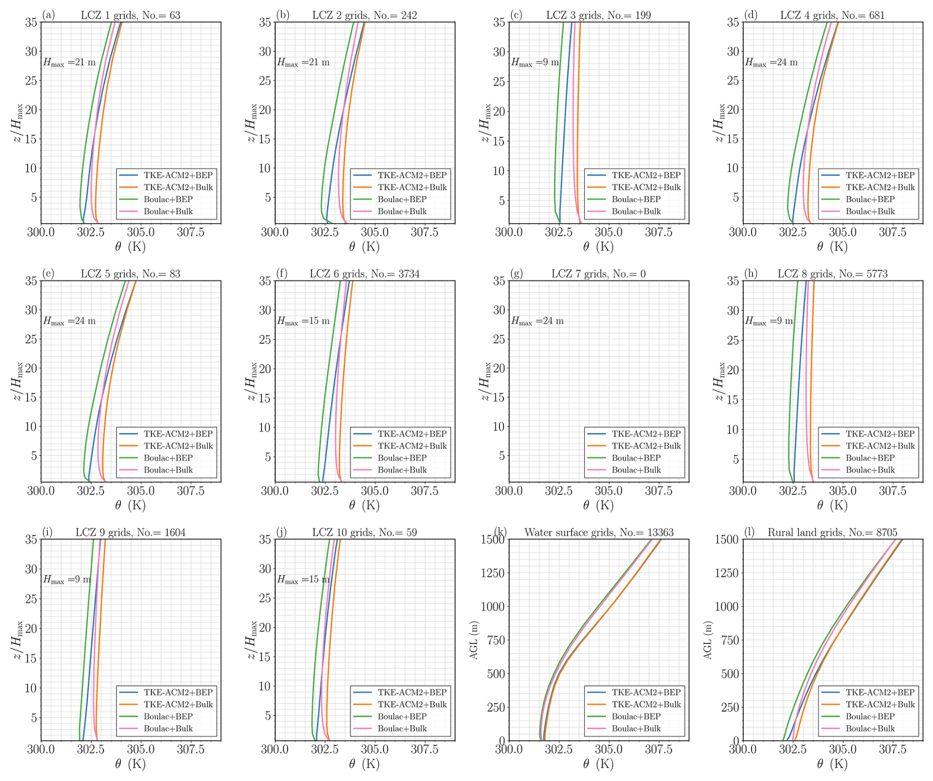
Figure C1 (a–j) Monthly mean vertical profiles of θ over LCZ 1–10; (k) over water surfaces; (l) over rural land cover.

Figure C2 Same as Fig. C1 but for U.

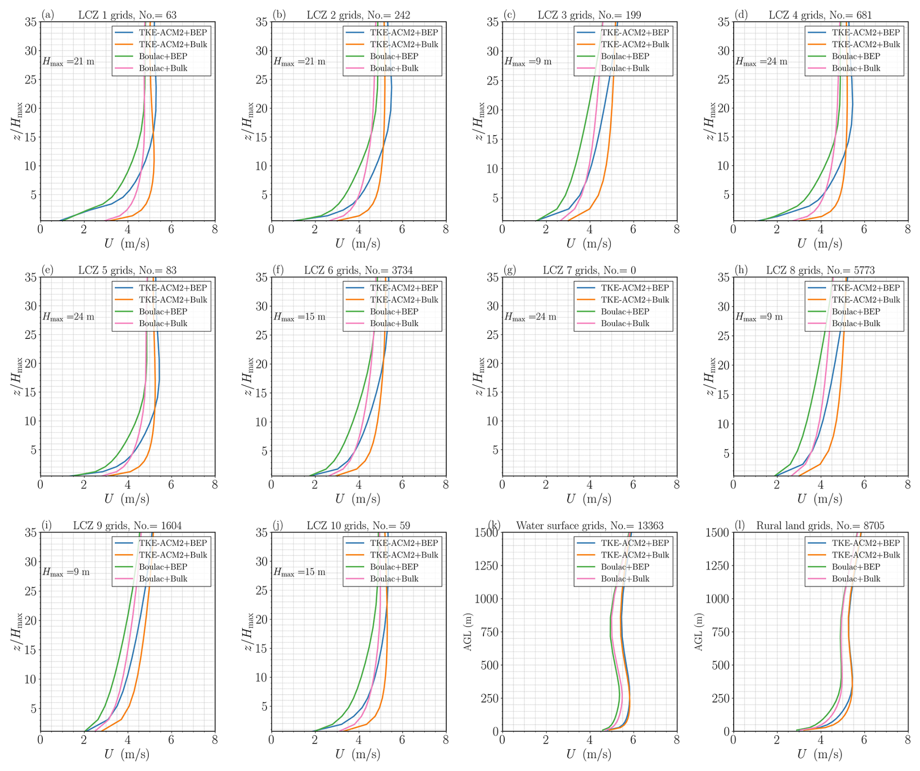
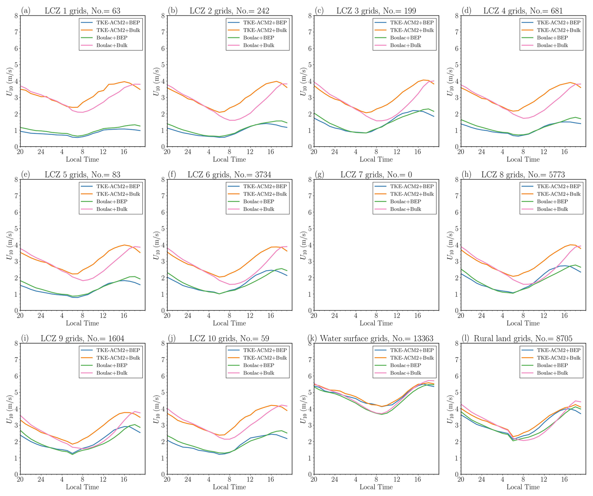
Figure C3 (a–j) Monthly mean U₁₀ over LCZ 1–10; (k) over water surfaces; (l) over rural land cover.

Figure C4 Same as Fig. C3 but for T₂.

Figure C5 Same as Fig. C3 but for RH₂.