HAPI2LIBIS (v1.0): a new tool for flexible high-resolution radiative transfer computations with libRadtran (version 2.0.5)

Atmospheric radiative transfer (RT) models are useful tools to increase our understanding of the physical interactions and processes occurring in the atmosphere and surface. In the category of free and open-source models, the library for radiative transfer (libRadtran) is a widely used and versatile package. However, running high-resolution calculations with libRadtran is often tedious since libRadtran does not include all the required information to run line-by-line executions (i.e., resolving individual spectral lines of gases) in a flexible way under specific atmospheric conditions, meaning that external software is required. This poses a problem for a user since generating necessary files for libRadtran requires familiarity with the topic of molecular spectroscopy in addition to knowing how to use the external software, which may not be tailored for producing libRadtran-compatible files. In this paper, we present HAPI2LIBIS, a compact software tool intended to be used in close connection with libRadtran to enable easy high-resolution calculations. HAPI2LIBIS streamlines the generation of high-resolution molecular absorption data for libRadtran by utilizing the latest version of the High-Resolution Transmission Molecular Absorption (HITRAN) database and the HITRAN Application Programming Interface (HAPI) with user-specified spectral ranges and atmospheric profiles. HAPI2LIBIS also stores computed absorption cross-sections in its dynamically constructed lookup table and includes an option for pressure- and temperature-dependent interpolation in order to accelerate subsequent simulations.

1 Introduction

Atmospheric radiative transfer (RT) models are crucial when investigating the many interactions between electromagnetic radiation and the Earth's atmosphere and surface. RT models are used to simulate the transfer of solar and thermal radiation in the atmosphere and are widely used in Earth observation research. These models are essential for multiple applications, from instrument calibration (Govaerts and Clerici, 2004) and simulation (Vicent et al., 2016) to atmospheric physics studies covering cloud (Alexandrov et al., 2012), aerosol (Dubovik and King, 2000; Hasekamp and Landgraf, 2005; Randles et al., 2013), volcanic ash (Kylling et al., 2015; Sellitto et al., 2016), and gas and trace gas remote sensing fields (Clough et al., 1992; Schwaerzel et al., 2020), as well as for the development of algorithms dedicated to the atmospheric correction process of airborne or satellite images (Richter and Schläpfer, 2013; Ju et al., 2012). One field of research where RT models are used extensively is satellite remote sensing. Satellite remote sensing provides valuable information about the Earth's land surface, ocean, vegetation, and atmosphere (Donlon et al., 2012). Since RT models are used to model and simulate satellite observations (Tenjo et al., 2017; Lajas et al., 2008), the significant increase in the spectral resolution of spectrometers in many planned satellite missions, such as the FLuorescence EXplorer (FLEX) (Drusch et al., 2017) and the Copernicus Anthropogenic Carbon Dioxide Monitoring (CO2M) (Sierk et al., 2021) missions, imposes higher demands on current RT models.

Many RT models have been developed over the last few decades, with gradual increases in their modeling capabilities and their complexity over time. Some of the most well-known models include the MODerate resolution atmospheric TRANsmission (MODTRAN) (Berk et al., 2014), the Second Simulation of a Satellite Signal in the Solar Spectrum (6S) (Vermote et al., 1997), the Matrix Operator MOdel (MOMO) RT code (Fell and Fischer, 2001), the Doubling-Adding KNMI (DAK) model (de Haan et al., 1987), the SCIATRAN software package (Rozanov et al., 2014), the Radiative Transfer for TOVS (RTTOV) model (Saunders et al., 2018), the line-by-line radiative transfer model (LBLRTM) (Clough et al., 2005), or the more recently developed Eradiate project (https://www.eradiate.eu/site/, last access: 13 October 2025). Among the open-source category of RT models, one widely used and extremely versatile RT model is the uvspec included in the library for radiative transfer (libRadtran) package (Mayer and Kylling, 2005; Emde et al., 2016).

The libRadtran software package consists of a set of programs to carry out RT calculations in the solar and thermal spectral regions. Some of the benefits of libRadtran compared to many other RT codes are that it is free and open-source; it includes polarization, several molecular absorption parameterizations, a collection of RT solvers, and a database of cloud and aerosol models; and it has an extensive and clear documentation (https://www.libradtran.org/doc/libRadtran.pdf, last access: 13 October 2025). While libRadtran offers a comprehensive suite of capabilities for RT simulations, its usability and, therefore, flexibility are more limited when the user wishes to run high-spectral-resolution simulations. By default, libRadtran relies on band parameterizations, mainly the representative wavelengths absorption parameterization (REPTRAN) (Gasteiger et al., 2014), when computing molecular absorption by atmospheric gases. The REPTRAN parameterization includes three different bandwidths, which are defined at a coarse-resolution option of 15 cm⁻¹ width, a medium option of 5 cm⁻¹ width, and a fine option of 1 cm⁻¹ width. While REPTRAN satisfies the resolution requirements for many applications, it is not suitable for high-resolution simulations (sub-1 cm⁻¹ spectral resolution) due to the inability to discern subtle absorption line differences. By using a user-defined molecular absorption data file that is computed with a line-by-line model, i.e., highly resolved spectral calculations, and that is compatible with libRadtran, it would be possible to increase the desired spectral resolution of libRadtran RT calculations. Unfortunately, libRadtran does not include a line-by-line model by default. To overcome this limitation, the download section of the libRadtran website offers pre-computed line-by-line absorption data files covering the spectral range from 500 nm to 100 µm for the six standard atmosphere files defined in Anderson et al. (1986). These absorption datasets were computed using the RT code GENLN2 (Edwards, 1992) with molecular spectroscopic data from the High-Resolution Transmission Molecular Absorption (HITRAN) database (Gordon et al., 2022) using data from the older 1996 version (Rothman et al., 1998). Thus, the potentially outdated nature of these absorption data files derived from old HITRAN versions and available only for six pre-defined models of the atmosphere limits the potential simulation accuracy to be achieved. Besides the possible accuracy limitation, the generation and use of these auxiliary files can make running high-spectral-resolution simulations with libRadtran an arduous task.

In this context, several programs have been developed to enable high-resolution calculations with libRadtran. For example, the widely used Atmospheric Radiative Transfer Simulator (ARTS) model (Buehler et al., 2005; Eriksson et al., 2011; Buehler et al., 2018), which is a comprehensive tool used for atmospheric radiative transfer applications, can be used to compute molecular absorption files for libRadtran. Another tool available for this purpose is the Python scripts for Computational ATmospheric Spectroscopy (Py4CAtS) (Schreier et al., 2019). However, these tools might be cumbersome for new and occasional users due to the extensive options provided by these sophisticated RT codes, the formalism required in input and output files, and the possible requirement for users to download beforehand the spectroscopic data from HITRAN or from other spectroscopic data sources.

To make libRadtran a more versatile program for high-spectral-resolution RT calculations by easing the simulation process, including high-spectral-resolution data, we present HAPI2LIBIS. HAPI2LIBIS is a Python-based software that uses the HITRAN Application Programming Interface (HAPI) (Kochanov et al., 2016) as its core to compute molecular absorption files that are compatible with libRadtran. HAPI is a software framework that enables users to access, download, and work with the latest data from the HITRAN database (https://hitran.org/hapi/, last access: 13 October 2025) by providing a standardized and convenient way to extract spectral molecular data, thus increasing the functionality of the HITRAN database. In addition to HITRAN data, HAPI2LIBIS can utilize measured absorption cross-section data files that are included in libRadtran or provided by the user. These files can be used to complement some gas absorption calculations where HITRAN data are unavailable. The main purpose of HAPI2LIBIS is to enable high-resolution RT calculations with libRadtran for users that require a higher spectral resolution than REPTRAN can provide (i.e., finer than 1 cm⁻¹) and for users who want to use the latest HITRAN data for line-by-line computations with different atmospheric gas constituents and profiles. These capabilities are particularly valuable for studies involving detailed molecular spectroscopy, where accurate representation of absorption lines is critical, as well as for high-resolution instrument development or characterization studies. While the HITRAN database contains data on absorption cross-sections, collision-induced absorption, and the water vapor continuum absorption, the current focus of the HAPI2LIBIS is to obtain the line-by-line data from HITRAN and to compute the cross-sections locally.

We have also included in HAPI2LIBIS the possibility of utilizing irregular interpolation methods to provide significant computational speed-ups without sacrificing too much accuracy. This option can be highly valuable, for example, when multiple runs with similar atmospheric conditions must be modeled since previously computed data can be reused so that the introduced interpolation error is minimal compared to the other error sources, such as sensor noise. Therefore HAPI2LIBIS could be used as part of a retrieval algorithm when the forward model requires line-by-line calculations. HAPI2LIBIS could act as a replacement for precomputed spectral absorption tables, such as ABSCO (Payne et al., 2020) in the case of the total column of CO₂ retrievals, or it could conveniently complement a retrieval algorithm where gas absorption cross-sections are computed as a part of the retrieval algorithm, such as in the CH₄ profile retrieval of SWIRLAB (Tukiainen et al., 2016). As HAPI2LIBIS is used before an RT model is run, it can be utilized simultaneously with spectral RT optimization methods, such as correlated-k (Kato et al., 1999), low-streams interpolation (O'Dell, 2010), or machine-learning-based approaches (e.g., Su et al., 2023; Mauceri et al., 2022).

The remaining part of this work is structured as follows: Sect. 2 provides a detailed overview of the HAPI2LIBIS software package and its use together with libRadtran. Section 3 details, with practical examples, how to make use of HAPI2LIBIS and assess its performance against simulations done in libRadtran using REPTRAN. Additionally, Sect. 3 presents an example of the HAPI2LIBIS cross-section interpolation feature that is included to significantly speed up the computations between similar pre-computed atmospheric files. Finally, conclusions are provided in Sect. 4.

2 HAPI2LIBIS: connecting HITRAN, HAPI, and libRadtran

2.1 Installation and usage

The requirements to run HAPI2LIBIS are Python 3 and NumPy (Harris et al., 2020), SciPy (Virtanen et al., 2020), PyYAML, and NetCDF (Rew and Davis, 1990; Brown et al., 1993) modules. Additionally, an internet connection is required to access the latest HITRAN data. The recommended operating systems to run HAPI2LIBIS are GNU/Linux and macOS systems. Python knowledge is recommended but not required to run HAPI2LIBIS successfully. It is possible to run HAPI2LIBIS without libRadtran installation, but it is not recommended since it would severely limit the functionality of HAPI2LIBIS.

HAPI2LIBIS software can be downloaded from GitHub (https://github.com/amikko/hapi2libis, last access: 13 October 2025) with an MIT license. The software consists of a Python file called hapi2libis.py and a human-readable text setting file written in yaml. HAPI2LIBIS also requires the hapi.py file, which is obtainable from GitHub (https://github.com/hitranonline/hapi, last access: 13 October 2025) and from the HITRAN webpage (https://hitran.org/hapi/, last access: 13 October 2025). The easiest way to install HAPI2LIBIS is to place both of the files, i.e., hapi2libis.py and hapi.py, into the same folder.

HAPI2LIBIS can be operated from the command line with the command python hapi2libis.py config.yaml, where config.yaml contains all the settings required by HAPI2LIBIS. The settings file contains a section for basic options that the user should edit for their local specification and simulation needs. The settings file also contains a section for advanced options, including features for advanced users and for those who might wish to edit the hapi2libis.py script to be more suitable for their specific needs. The basic options are listed in Table 1.

Table 1 Description of the basic parameters in the settings file.

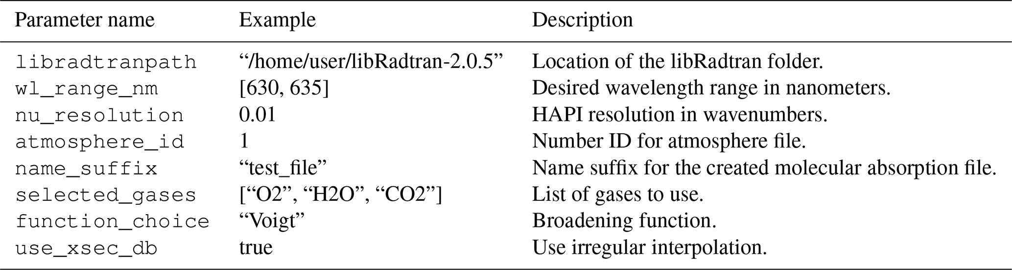
Before running HAPI2LIBIS for the first time, the user should modify the settings file. The minimum recommended settings that the user should modify to successfully run HAPI2LIBIS is the file path pointing to the libRadtran folder (e.g., libradtranpath: '/home/user/bin/libRadtran-2.0.5'), the desired atmosphere file from the ones provided by libRadtran (Anderson et al., 1986), the wavelength range for the computation, and the desired resolution for the output molecular absorption file.

The general workflow of HAPI2LIBIS is presented in Fig. 1. In the initialization phase, the yaml settings file is read following the download of the latest spectroscopy information from the HITRAN database for the required gases in the specified spectral range. Based on the downloaded gases, HAPI2LIBIS will initiate the main computation loop where the absorption coefficients will be computed for every atmospheric layer defined by the model of the atmosphere selected from the libRadtran-included defaults by Anderson et al. (1986) or as defined by the user. Finally, the molecular absorption file (input for libRadtran) is generated.

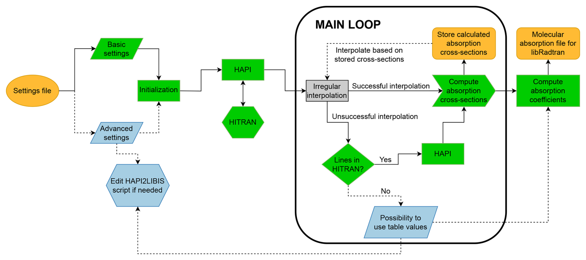
Figure 1 Flowchart visualizing the general phases of HAPI2LIBIS. The orange-colored shape for the settings file denotes the start of the flowchart, while the green-colored shapes show the regular flow. The blue-colored shapes show the processes that require using the advanced options. The gray shape in the middle shows the location of the option to speed up computations if the irregular interpolation is activated. Finally, the orange shapes at the end of the flowchart (top right) denote the output files of HAPI2LIBIS.

2.2 The main computation sequence

The easiest way to run HAPI2LIBIS is to use one of the six standard atmosphere files that are included in libRadtran. These files consist of rows and columns, with each row corresponding to an atmospheric level, while the columns correspond to different parameters. The parameters are altitude above sea level, pressure, temperature, air concentration, and different gas concentrations. The gases included in these files are ozone (O₃), oxygen (O₂), water vapor (H₂O), carbon dioxide (CO₂), and nitrogen dioxide (NO₂). Additionally, auxiliary gases from the US standard atmosphere can be used, and their concentration profiles are included in separate files in libRadtran. These are methane (CH₄), nitrous oxide (N₂O), carbon monoxide (CO), and nitrogen (N₂). However, for advanced users, HAPI2LIBIS can also read custom atmosphere files that are constructed similarly to the standard atmosphere files provided that the file contains columns for altitude (km), pressure (hPa), temperature (K), and number concentration of air (cm⁻³). The additional columns should have the profiles for user-specified gases in the same units as the number concentration of air (cm⁻³). The column order of the user-specified gases is not fixed, but the gas concentration should be detailed in rows in altitude top-down order, and the units must be the same as in the standard files. For available gases to use in computations, we refer the reader to the HITRAN website (https://hitran.org/lbl/, last access: 13 October 2025).

HAPI2LIBIS will compute absorption cross-sections of each of the gases specified in the settings file using the pressures, temperatures, and gas concentrations defined in the atmosphere file for each of the atmospheric layers. Since the atmosphere file consists of n number of levels, HAPI2LIBIS will compute, by default, the properties of n−1 atmospheric layers, where one atmospheric layer consists of two consecutive rows in the atmosphere file, as per the atmospheric definition formalism in libRadtran. This process is referred to as the main loop (see Fig. 1).

The first step in the main loop is computing the layer altitude and thickness, where the user can choose in the settings file if the atmospheric parameters should be interpolated to the mean altitude of the layer. Without altitude interpolation, HAPI2LIBIS uses the lower altitude row values from the atmosphere file to compute the layer properties. For example, a layer from 0 to 1 km will use the values from the row corresponding to 0 km, while a layer from 1 to 2 km will use the values from the row corresponding to 1 km and so forth for the rest of the layers. With the altitude interpolation option enabled, HAPI2LIBIS assumes that the row values in the atmosphere file correspond to the values at the given altitude. Therefore, to compute the layer properties, HAPI2LIBIS will interpolate the values in the atmosphere file to the layer mean altitude. Compared to the previous example, now, a layer from 0 to 1 km will use the interpolated values corresponding to an altitude of 0.5 km, while a layer from 1 to 2 km will use the interpolated values corresponding to an altitude of 1.5 km and so forth for the rest of the layers. The option to control this is the parameter interpolate_to_layer_midpoint in the settings file, where the value true means that the interpolated values are used.

Once the layer properties for layer l are computed, HAPI2LIBIS will move to the second step in the main loop and compute the mixing ratios for every used gas using the following equation:

$$\begin{array}{}\text{(1)}& {\mathit{\xi }}_{\mathrm{gas}}\left(l\right)={\displaystyle \frac{c_{\mathrm{gas}}\left(l\right)}{c_{\mathrm{air}}\left(l\right)}},\end{array}$$

where ξ_gas denotes the mixing ratio of a gas in layer l, c_gas denotes the concentration of a gas in layer l, and c_air denotes the concentration of air in layer l. These mixing ratios are later used to communicate to HAPI the gas mixture composition, which affects the air- and self-broadening parameters during the computation of absorption cross-sections.

In the third step of the main loop, HAPI2LIBIS will compute the absorption cross-sections for every gas used. This step is usually the slowest one, where the majority of the total computation time will be spent. The cross-sections are computed in the wavelength range specified in the settings file's wl_range_nm parameter, with a wavenumber step option nu_resolution. The broadening function HAPI2LIBIS uses can be set in the settings file where the possible functions to use are listed in the HAPI manual (https://hitran.org/static/hapi/hapi_manual.pdf, last access: 13 October 2025). The function choices are Voigt profile (Voigt), Lorentzian profile (Lorentz), speed-dependent Voigt profile (SDVoigt), Doppler profile (Doppler), and Hartmann–Tran profile (HT). The broadening function accounts for air- and self-broadening, where air-broadening refers to the widening of spectral lines caused by collisions between the absorbing gas and surrounding atmosphere, while self-broadening refers to widening due to collisions between molecules of the same gas.

HAPI2LIBIS will utilize HAPI to compute cross-sections for gases downloaded from HITRAN in the initialization phase. The cross-sections are computed one by one, where HAPI's diluent self parameter is set to the mixing ratio of the gas being computed, while the diluent air is set to the difference between unity and the mixing ratio of the gas being computed.

From the computed cross-sections, HAPI2LIBIS will compute the gas mixture's total absorption coefficient and use that to compute the optical depth of the atmospheric layer l. The total absorption coefficient σ_abs is computed with the following equation:

$$\begin{array}{}\text{(2)}& {\mathit{\sigma }}_{\mathrm{abs}}\left(l\right)=\sum _{\mathrm{gas}}{Q}_{\mathrm{gas}}\left(l\right)\cdot c_{\mathrm{gas}}\left(l\right),\end{array}$$

where Q_gas is the computed absorption cross-section for a gas. Now, the optical depth of the layer l can be computed with the following equation:

$$\begin{array}{}\text{(3)}& \mathit{\tau }\left(l\right)={\mathit{\sigma }}_{\mathrm{abs}}\left(l\right)\cdot z\left(l\right),\end{array}$$

where τ denotes the optical depth of the layer, and z denotes the layer thickness. Finally, HAPI2libis will save the computed values in a NetCDF file specified by hapi2libis_mol_tau_file.nc, which libRadtran is able to use with the libRadtran input option mol_tau_file abs hapi2libis_mol_tau_file.nc.

2.3 Storing calculated absorption cross-sections and their irregular grid interpolation

The calculated absorption cross-sections are stored by default in a NetCDF file for a particular gas, wavelength band, and wavenumber resolution. NetCDF is a widely used data format due to its ability to efficiently store large datasets with multi-dimensional arrays. Utilizing NetCDF files allows HAPI2LIBIS to save and retrieve computed absorption cross-sections efficiently, minimizing storage requirements while ensuring data integrity. The file can store the absorption cross-sections for different temperature (T), pressure (p), and gas partial pressure combinations (p_g). To further reduce the computational weight of absorption cross-section calculations, HAPI2LIBIS enables interpolation in the $(T,p,p_{\mathrm{g}})$ parameter space. Two irregular interpolation schemes are available: nearest-neighbor and bounding-box interpolation.

Both of these two interpolation methods depend on a concept of a metric (distance function) in the $(T,p,p_{\mathrm{g}})$ space. The metric used in HAPI2LIBIS to compute the distance d_w between two points ${\mathit{r}}_i=(T_i,p_i,p_{gi})$ and ${\mathit{r}}_j=(T_j,p_j,p_{gj})$ is

$$\begin{array}{}\text{(4)}& d_w({\mathit{r}}_i,{\mathit{r}}_j)=({\mathit{r}}_j-{\mathit{r}}_i{)}^{\mathrm{T}}\mathbf{W}({\mathit{r}}_j-{\mathit{r}}_i),\end{array}$$

where $\mathbf{W}\in {\mathbb{R}}^{\mathrm{3}\times \mathrm{3}}$, and $\mathbf{W}=\mathrm{diag}(w_{\mathrm{1}},w_{\mathrm{2}},w_{\mathrm{3}})$. The values w₁, w₂, and w₃ can be different for each gas, wavenumber region, spectral resolution, broadening function, and pressure and temperature used. For a particular dataset consisting of points ${\mathit{r}}_i=(T_i,p_i,p_{gi}),$ $i=\mathrm{0},\mathrm{1},\mathrm{\dots },n$, the weighting matrix W is

$$\begin{array}{}\text{(5)}& \begin{array}{rl}& \mathbf{W}=\\ & \left[\begin{array}{ccc}(max\mathit{\{}{T}_i\mathit{\}}-min\mathit{\{}{T}_i\mathit{\}}{)}^{-\mathrm{2}}& \mathrm{0}& \mathrm{0}\\ \mathrm{0}& (max\mathit{\{}{p}_i\mathit{\}}-min\mathit{\{}{p}_i\mathit{\}}{)}^{-\mathrm{2}}& \mathrm{0}\\ \mathrm{0}& \mathrm{0}& (max\mathit{\{}{p}_{gi}\mathit{\}}-min\mathit{\{}{p}_{gi}\mathit{\}}{)}^{-\mathrm{2}}\end{array}\right].\end{array}\end{array}$$

To interpolate point $\mathit{r}=(T,p,p_{\mathrm{g}})$, an inverse distance weighting method (Franke, 1982) is used. The described method is modified by not using all of the points in the dataset but rather using only two: r_i and r_j. These two points are selected from a subset $C=\mathit{\left\{}{\mathit{r}}_i\right|i\in \mathrm{0},\mathrm{1},\mathrm{\dots },n\wedge d_w(\mathit{r},{\mathit{r}}_i)<d_c\mathit{\}}$, where d_c threshold value is selected such that $\left|C\right|=n_c$, for which n_c is chosen arbitrarily beforehand. In other words, these two points are picked from n_c closest points to r. The two points must also fulfill the following criteria:

1. $\min (T_i,T_j)<T<\max (T_i,T_j)$,

2. $\min (p_i,p_j)<p<\max (p_i,p_j)$,

3. $\min (p_{gi},p_{gj})<p_{\mathrm{g}}<\max (p_{gi},p_{gj})$,

4. $v({\mathit{r}}_i,{\mathit{r}}_j)<v_{\max }$, and

5. $v({\mathit{r}}_i,{\mathit{r}}_j)<=v({\mathit{r}}_i^{\prime },{\mathit{r}}_j^{\prime })\forall {\mathit{r}}_i^{\prime },{\mathit{r}}_j^{\prime }\in C$,

where

$$\begin{array}{}\text{(6)}& v=\det \left(\mathrm{diag}\right(\mathbf{W}\left[\right|T_i-T_j|,|p_i-p_j|,|p_{gi}-p_{gj}\left|{]}^{\mathrm{T}}\right))\end{array}$$

is the volume of the box defined by the points r_i and r_j in the d_w metric. More simply put, the interpolant must be contained in the box defined by r_i and r_j, the box volume must be less than a predetermined threshold value, and the selected box must be the smallest box in the set C.

With suitable r_i and r_j, the interpolated absorption cross-section Q_gas at the point r is

$$\begin{array}{}\text{(7)}& Q_{\mathrm{gas}}\left(\mathit{r}\right)={\displaystyle \frac{Q_{\mathrm{gas}}\left({\mathit{r}}_i\right)d_w(\mathit{r},{\mathit{r}}_j)+Q_{\mathrm{gas}}\left({\mathit{r}}_j\right)d_w(\mathit{r},{\mathit{r}}_i)}{d_w(\mathit{r},{\mathit{r}}_j)+d_w(\mathit{r},{\mathit{r}}_i)}}.\end{array}$$

2.4 Extending HITRAN with auxiliary tables from libRadtran

The HITRAN database does not cover all of the wavelengths where significant molecular absorption is encountered in the atmosphere. For example, the Chappuis band of O₃, which covers the wavelength range between 400 and 650 nm, cannot be downloaded from the HITRAN database. We note that libRadtran manages this by including several measured absorption cross-section files below 1130 nm for O₃ and NO₂ and for O₂–O₂ collision pairs.

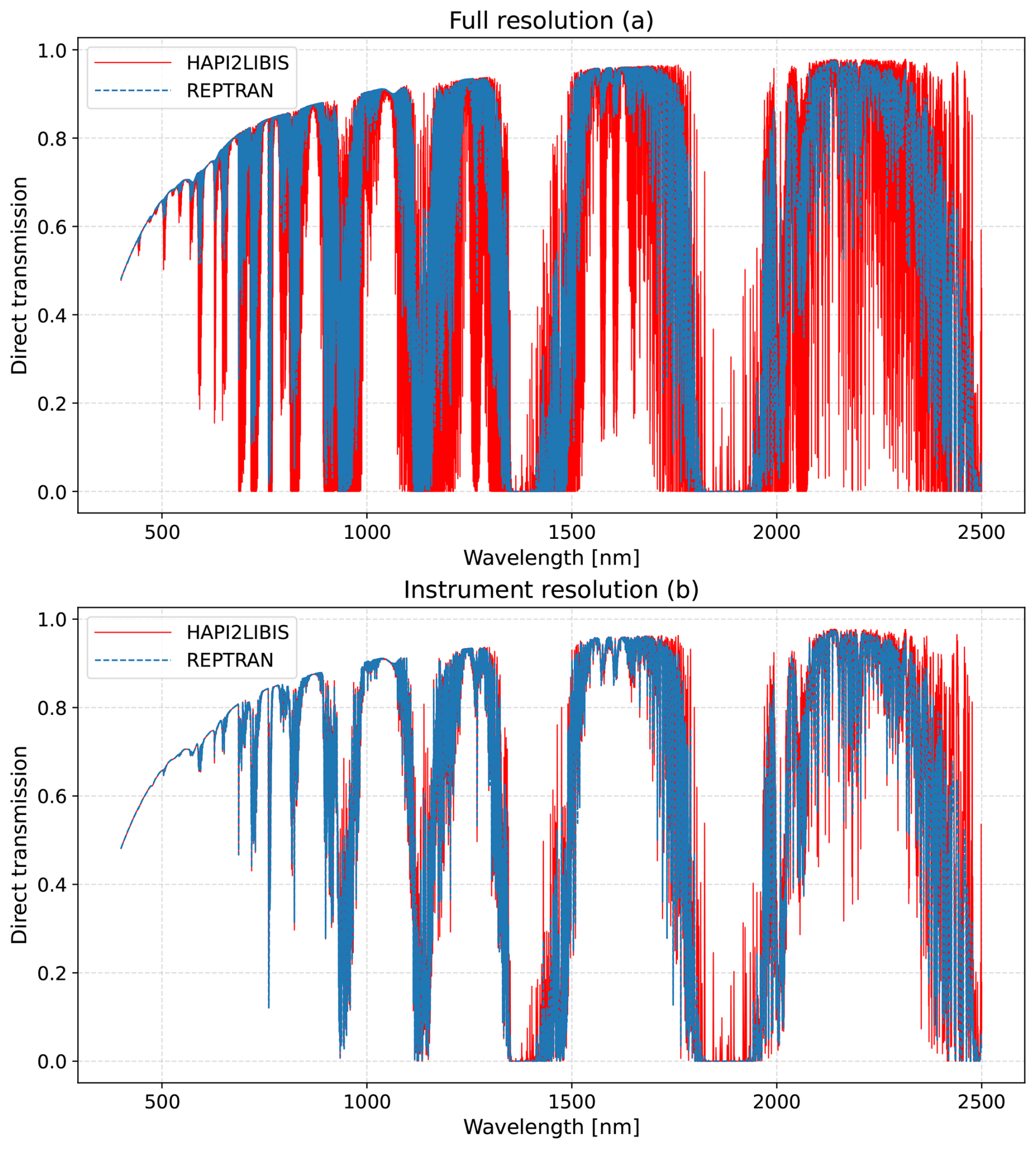
Figure 2 Comparison of simulated direct transmission from sun to surface at full (a) and instrument (b) resolution with a HAPI2LIBIS-generated molecular absorption optical depth file against a REPTRAN fine-molecular-absorption parameterization. The instrument response function was a triangular-slit function with a full width at half maximum (FWHM) of 0.3 nm.

To make HAPI2LIBIS comparable to the highest-resolution option of REPTRAN, we have included in HAPI2LIBIS the possibility of using some of the measured absorption cross-section files included in libRadtran (Emde et al., 2016). The measured absorption cross-section table values are used as per the instructions in the file. This means that they may lack pressure and temperature effects. The values are interpolated to the requested wavelength range and resolution, meaning that no line-broadening effects are applied. For O₃, the available files are molina (Molina and Molina, 1986), bass_and_paur (Bass and Paur, 1985), daumount (Daumont et al., 1992), and bogumil (Bogumil et al., 2003). For NO₂, the available files are burrows (Burrows et al., 1998) and bogumil (Bogumil et al., 2003). For O₂–O₂, the only available file is greenblatt (Greenblatt et al., 1990).

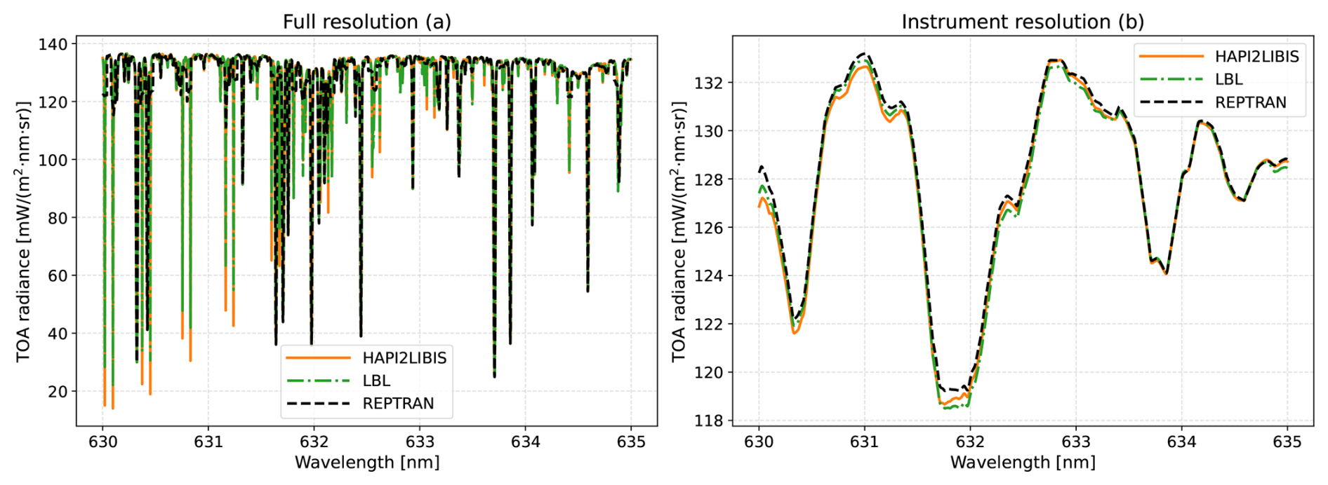
Figure 3 Simulated TOA radiance at full (a) and instrument (b) resolution using REPTRAN, HAPI2LIBIS, and line-by-line molecular absorption data files provided on the libRadtran webpage. The atmospheric simulation includes O₂, H₂O, and CO₂.

3 Model comparison results

3.1 Comparison of libRadtran simulations

For this section's results, the libRadtran simulation specifications are fixed to the following defaults unless otherwise stated. For the measurement geometry, the solar zenith angle and the surface albedo values were set to 35° and 0.3, respectively. The atmosphere chosen was the mid-latitude summer. The atmosphere contains default-type aerosols in accordance with Shettle (1990), corresponding to spring–summer conditions with a visibility of 50 km, and rural-type aerosols in the lower 2 km of the atmosphere and background-type aerosols above 2 km in the atmosphere. These simulation parameters were chosen since they represent typical mid-latitude summer conditions, which are commonly used as a benchmark in atmospheric radiative transfer studies.

The output spectral resolution in libRadtran is usually defined by the chosen extraterrestrial spectrum. We decided to use the full-resolution spectrum according to Kurucz (1992), which can be downloaded from the libRadtran webpage. Concerning HAPI2LIBIS, we used every available isotope for the downloaded HITRAN gases and the default auxiliary tables for O₃, NO₂, and O₂–O₂, namely molina, burrows, and greenblatt, respectively. The broadening function was set as Voigt, and the wavenumber resolution was 0.01 cm⁻¹.

Figure 2 shows libRadtran-simulated direct transmission results when using the REPTRAN fine-molecular-absorption parameterization (1 cm⁻¹) and the HAPI2LIBIS molecular absorption file with a full resolution (a) and a simulated instrument resolution (b). The instrument spectra are computed by convolving the full-resolution spectra with a triangular-slit function with a full width at half maximum (FWHM) of 0.3 nm, which represents a typical high-resolution instrument. The trace gases that were included in the simulations were O₃, O₂, H₂O, CO₂, NO₂, CH₄, N₂O, CO, N₂, and O₂–O₂. The figure shows the higher resolution of HAPI2LIBIS compared to REPTRAN, which is as expected since REPTRAN is not a line-by-line method and places greater priority on simulation speed over accuracy. The differences in spectral resolution between HAPI2LIBIS and REPTRAN are particularly noticeable in the 2000–2500 nm range, where HAPI2LIBIS shows many of the finer absorption lines that are missing in the REPTRAN data. For easier comparison, Figs. A1 and A2 in Appendix A show difference plots of the results shown in Fig. 2. The libRadtran simulation to generate the spectra shown in Fig. 2 took around 13 min with REPTRAN and around 92 min with HAPI2LIBIS (single thread on Intel^® Xeon^® Gold 6230 CPU, 2.1 GHz, 64 GB memory).

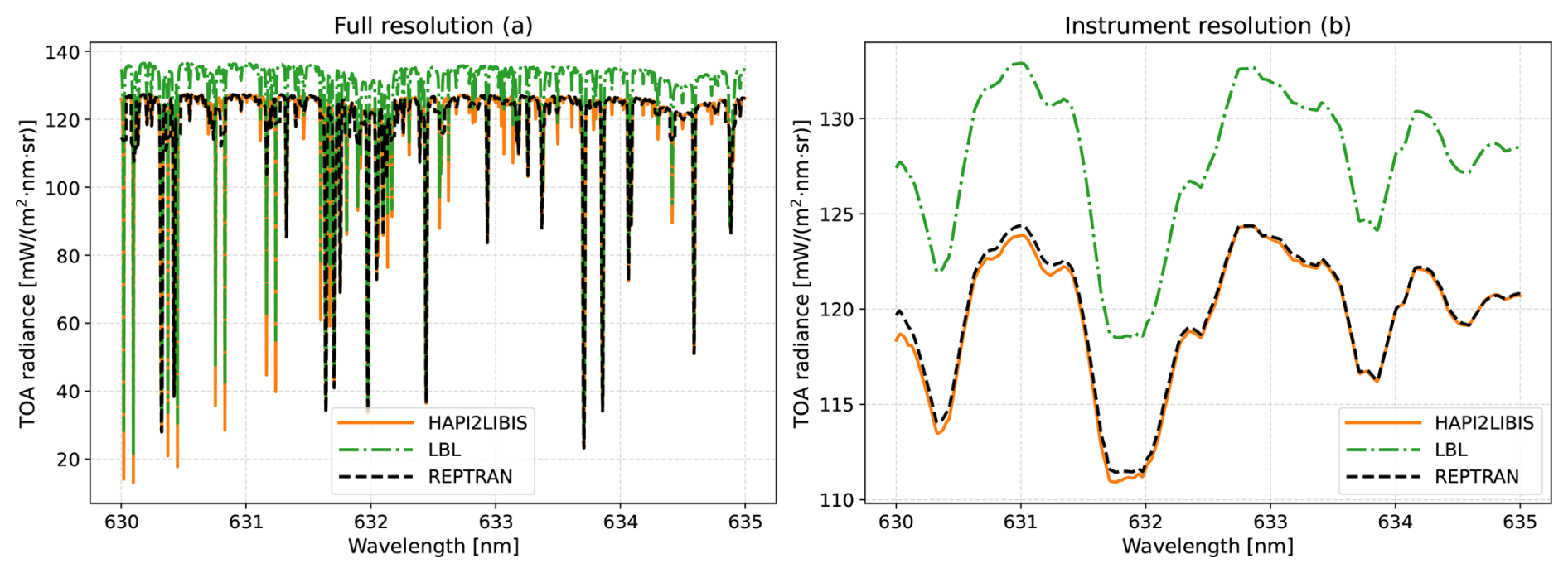
Figure 4 Simulated TOA radiance at full (a) and instrument (b) resolution using REPTRAN, HAPI2LIBIS, and line-by-line molecular absorption data files as provided on the libRadtran webpage. The distinction compared to the results shown in Fig. 3 is that, now, the atmospheric O₃ is included in the simulations.

Figure 3 shows simulated top-of-atmosphere (TOA) radiance results with full (a) and instrument (b) resolution using libRadtran paired with the REPTRAN fine-molecular-absorption parameterization, the HAPI2LIBIS molecular absorption file, and the line-by-line absorption data that can be downloaded from the libRadtran webpage. The observing instrument has nadir view geometry. The trace gases that are present in the libRadtran line-by-line molecular absorption files are O₃, O₂, H₂O, CO₂, CH₄, N₂O, CO, and N₂, but for this specific example, the trace gases that were included in the simulation were O₂, H₂O, and CO₂. These gases were selected since they all appear in the HITRAN database for the requested wavelength range, meaning that the results are comparable. The figure shows that all three methods show major absorption lines at the same wavelengths, which is as expected. The figure also shows that REPTRAN has significantly smaller absorption spikes compared to the other two methods due to the coarser spectral resolution, while HAPI2LIBIS and line-by-line files provide similar results. The difference in the height of the spikes between HAPI2LIBIS and line-by-line files can be attributed to the different versions of HITRAN used (2020 and 1996) or to some possible differences in the used line-broadening function. The figure also shows that there is no substantial difference between the convolved lower-resolution spectra despite REPTRAN missing many of the absorption spikes; however, for high-resolution instrument data studies, these differences are significant.

Figure 4 shows the simulated TOA radiance results with full (a) and instrument (b) resolution when we include O₃ in the simulations that were presented in Fig. 3. Since the libRadtran line-by-line data files are based only on HITRAN data, which do not include O₃ at the chosen wavelengths, we can clearly see the difference in the TOA radiance between REPTRAN and HAPI2LIBIS compared to the libRadtran line-by-line data.

3.2 Comparison of interpolation methods

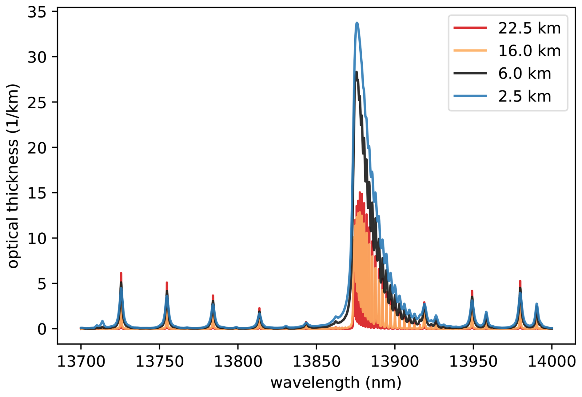
As a demonstration of the accuracy and speed of the irregular interpolation method, we processed 40 different atmospheric profiles used as priors in the Total Carbon Column Observation Network (TCCON) retrieval (Wunch et al., 2011). The prior profiles used are from the Sodankylä TCCON (Kivi et al., 2022) conducted from 1 March 2023 to 11 April 2023. Using the provided pressure, temperature profiles, and mixing profiles for CO₂, CH₄, and H₂O, the absorption cross-sections were computed in the 1600–1700 nm wavelength range. In that range, 36 765 discrete wavenumbers were used for calculating Voigt line shapes of 17 210, 12 858, and 3507 absorption lines for CO₂, CH₄, and H₂O, respectively. Each of the used atmospheres had 50 layers from 0 to 70 km and layer thicknesses from 0.42 to 2.38 km. As an example, Fig. 5 shows the optical densities used in this comparison exercise at different altitudes. To demonstrate HAPI2LIBIS capabilities in the thermal-infrared wavelength region, a similar example is presented in Fig. A3.

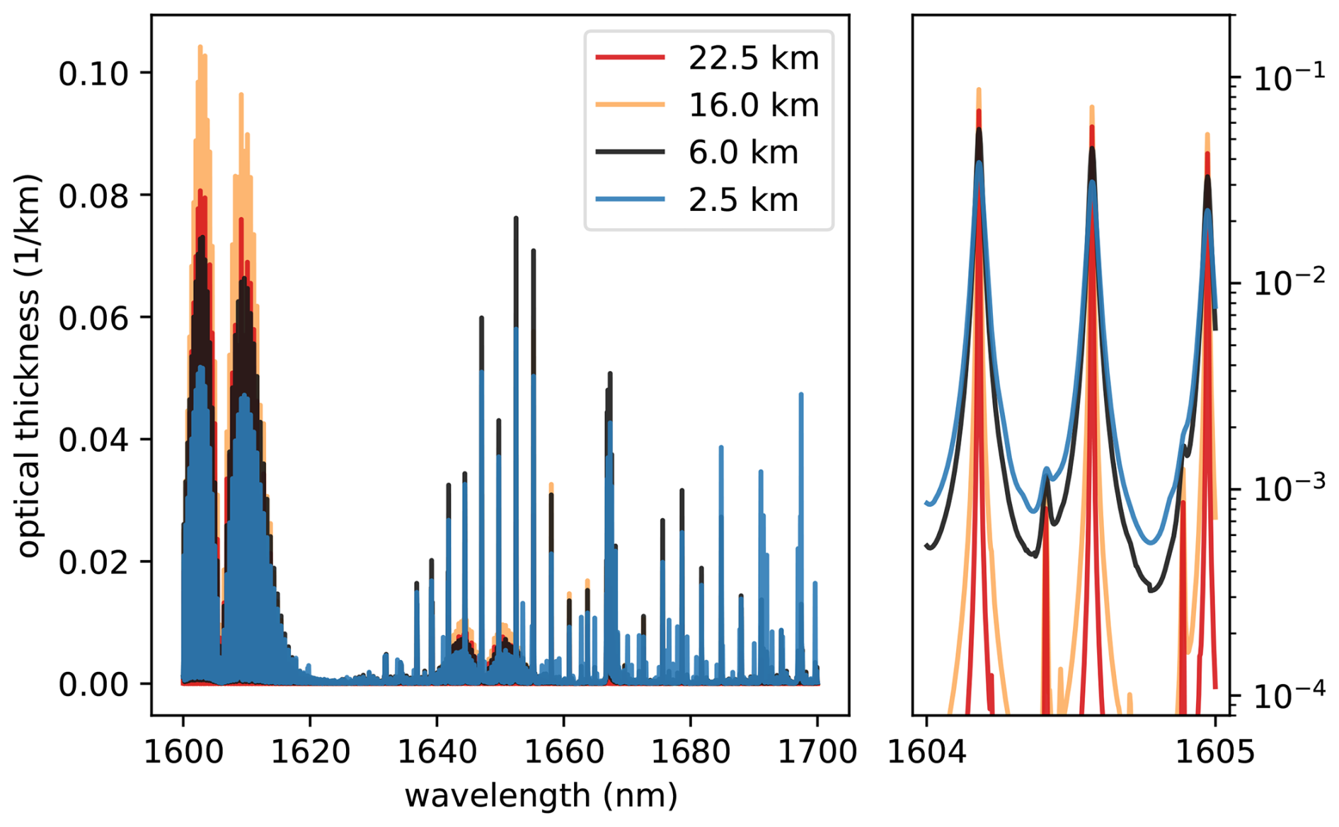
Figure 5 Examples of the fully computed total spectral optical densities used in interpolation comparison at different altitudes in the atmosphere from the first processed atmosphere (left) and the zoomed-in section to highlight the altitude dependence on the line shape (right). Contributions of CO₂, CH₄, and H₂O are aggregated together as this is the content of the mol_abs file created by HAPI2LIBIS.

In Fig. 6, the interpolation speed-ups with different interpolation schemes are compared to fully computing the cross-sections. The speed-up comparison was done on an Intel^® Core^™ i7-8650U CPU. Additionally, in Table 2, the file sizes of the accumulated databases after processing 40 atmospheres are presented.

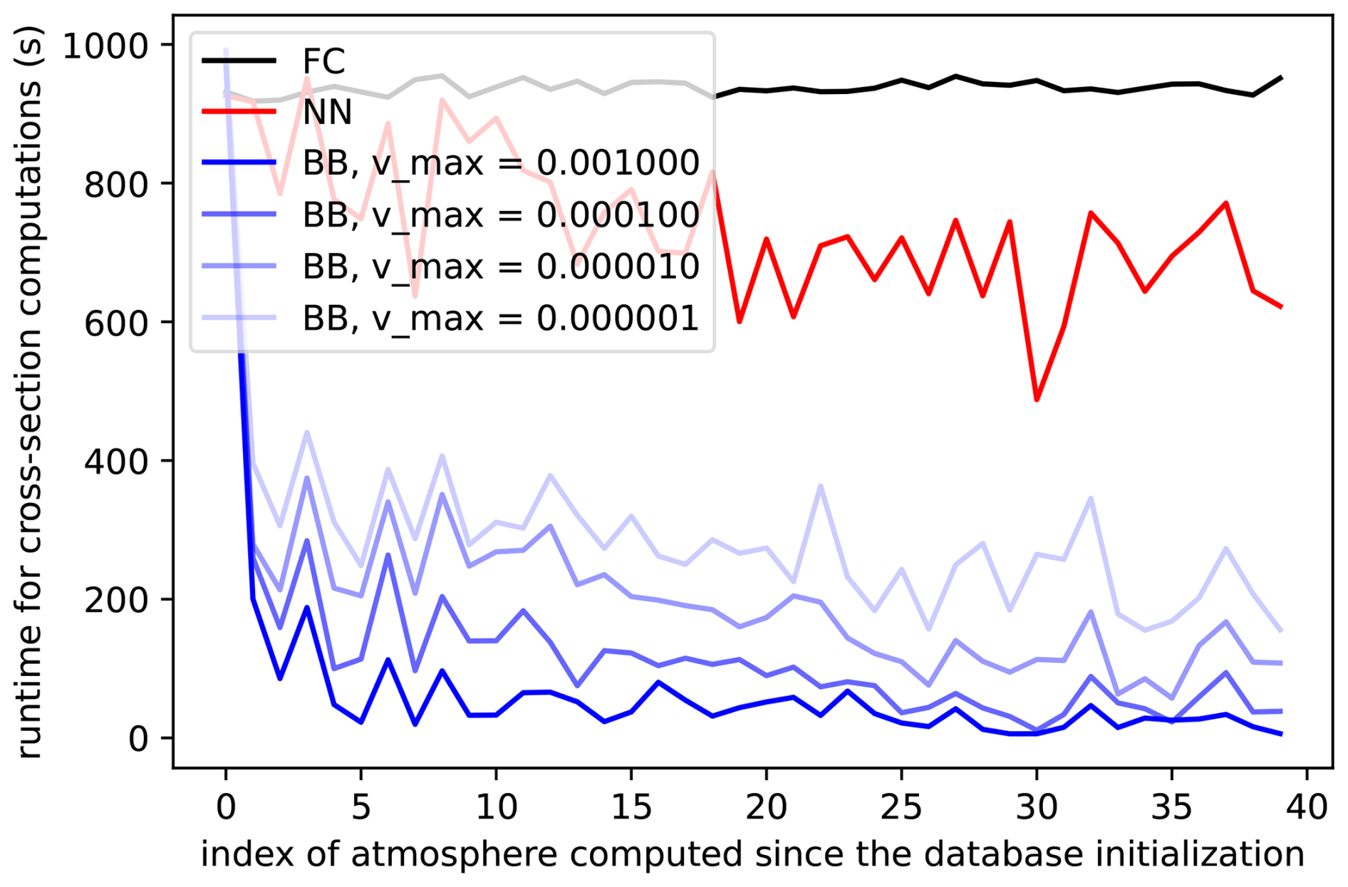
Figure 6 The runtime for processing the absorption cross-sections for each gas at every layer for a single atmosphere as a function of the amount of previously processed atmospheres. FC stands for full computation, NN stands for nearest neighbor, and BB stands for bounding box. The v_max parameter for NN is 0.01, and for BB it is included in the legend.

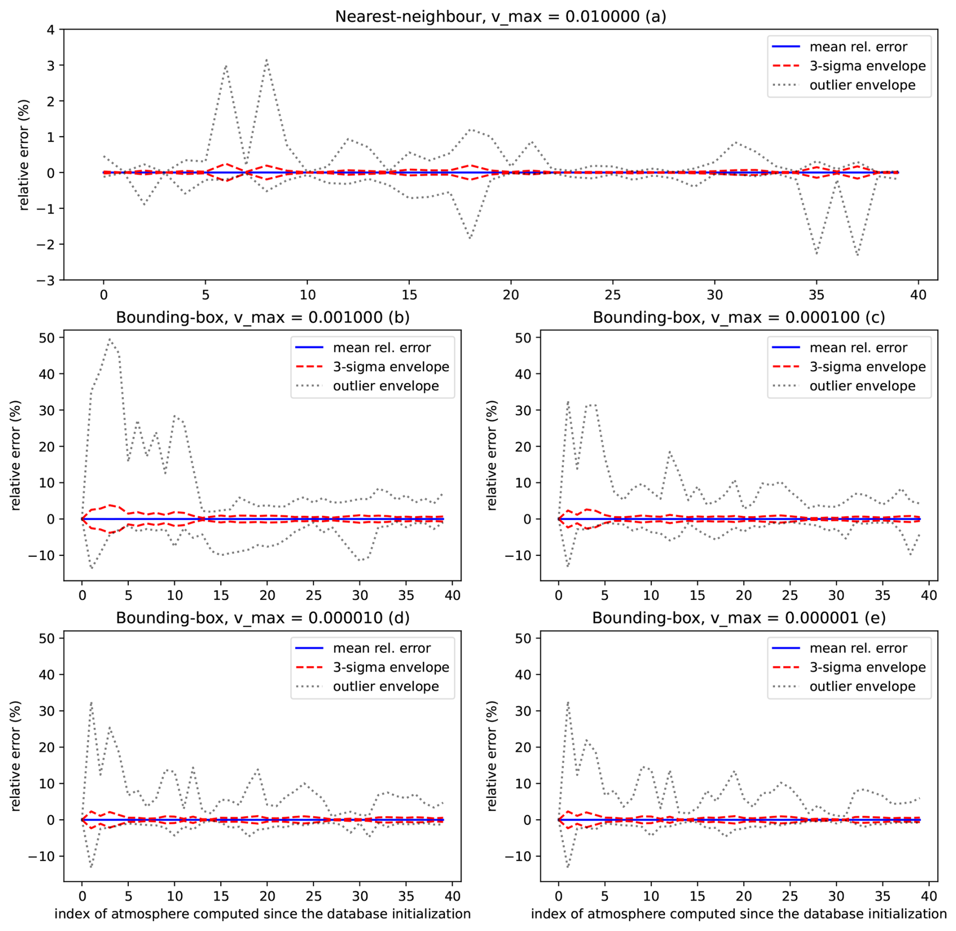
Figure 7 The relative error across the spectra for each interpolation method as a function of the number of previously processed atmospheres. The mean relative error is the solid blue line, the 3σ envelope (99.7 % of errors closer than mean when assuming normality) is the dashed red line, and all of the errors are contained within the dotted black line.

Table 2 The file sizes of the absorption cross-section databases after processing the 40 atmospheres.

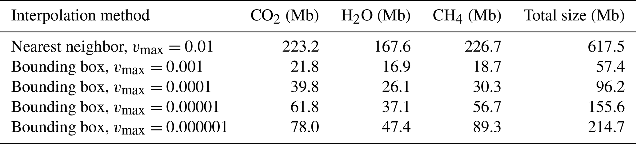
The interpolation methods decrease the runtime needed for absorption cross-section computations, as is apparent in Fig. 6, increasingly so when more atmospheres are computed. The bounding-box method enables 2- to 20-times-faster computation of the cross-sections, depending on the parameter. The nearest-neighbor method is also faster than the full computation, but the runtime reduction is hardly as drastic. The speed-up still increases since the runtime curves for interpolators have a downward trend. Since the interpolation methods accumulate the computed cross-sections into the database, it is reasonable that, with fewer interpolable cases, more would need to be computed and stored in the database, which is visible from Table 2. The total stored cross-section sizes ranging from 57.4 to 617.5 Mb for different interpolation methods show that the fastest method also requires the least disk space.

In Fig. 7, the relative error in the resulting transmittance is presented as a function of the atmospheric index for each interpolation method. The transmittance is computed with the following formula:

$$\begin{array}{}\text{(8)}& T\left(\mathit{\lambda }\right)=\exp \left(-\sum _{i=\mathrm{1}}^{\mathrm{50}}{l}_i{\mathit{\tau }}_i\left(\mathit{\lambda }\right)\right),\end{array}$$

where l_i is the thickness of the ith layer, and τ_i(λ) is the optical density at the ith atmospheric layer. In Fig. 7, the tradeoff in terms of accuracy versus computation speed is visible. Albeit requiring the most compute time and disk space, the nearest-neighbor method (a) performs consistently, with the largest outlier errors being 3 % for all 40 of the atmospheres. The bounding-box methods (b–e) can have outlier errors of up to 50 %, but the errors are reduced as more atmospheres are computed. The decrease in v_max from 0.001 to 0.0001 increases the accuracy, but reducing v_max more does not visibly increase accuracy further. The bounding-box method appears to require a burn-in period of about 15 atmospheres before the error distribution becomes somewhat stationary. After the burn-in period, the 3σ envelope ranges from 1 % to 2 %, signifying that almost all spectral points are accurately interpolated.

The requirement for the burn-in period can be explained by examining Eq. (5), which represents the full range of the data within the database. Before the database is adequately populated, the weighting matrix can cause the interpolation not to be strict enough, which results in higher errors. The large outlier errors can be explained by the linear nature of the bounding-box interpolation. Because the Voigt line shapes themselves are not linear with respect to p, T, or p_g, the linear interpolation can cause some unphysical peak shifts, which can result in large relative errors in transmittance, especially in the presence of fully saturated absorption lines. This can be a problem in all cases where linear interpolation of absorption cross-sections is done. However, in the use cases where spectral observations of specific instruments are simulated, the instrument line shape function can be broad enough to nullify the errors of these rare outliers.

4 Conclusions

In this paper, we presented HAPI2LIBIS, a Python-based tool designed to integrate HITRAN data with libRadtran by interfacing HAPI with the aim of enabling easy high-resolution radiative transfer calculations with libRadtran. To achieve this goal, HAPI2LIBIS has been made as interoperable with libRadtran as possible. With HAPI2LIBIS, the user is able to compute molecular absorption cross-sections of various gases for different atmospheric conditions from the ultraviolet to the microwave region.

In HAPI2LIBIS, the process of computing absorption cross-sections benefits from the high-precision molecular absorption line data available in the HITRAN database. Unlike some alternative strategies that rely on precomputed tables or band-parameterized models, HAPI2LIBIS calculates absorption cross-sections dynamically based on the gas concentrations in each atmospheric layer, thus improving the accuracy of the simulations.

The use of HAPI2LIBIS can be particularly useful for applications such as high-resolution instrument simulations and studies requiring precise representation of molecular absorption features. The cross-section interpolation database enables rapid processing of a series of atmospheres with only slight errors, as well as the boosting of repeated computational studies by conveniently storing the previously computed cross-sections.

As a final remark, most of the capabilities present in HAPI2LIBIS can be found in other sophisticated models. For example, both LBLRTM and Py4CAtS can compute absorption cross-sections of gases based on HITRAN data. However, the core design principle of HAPI2LIBIS is to add more functionality into libRadtran while being relatively easy to use. In future HAPI2LIBIS versions, planned updates include implementing parallel-computation techniques in the cross-section computation, utilizing more data from HITRAN than only the line-by-line data, and the option to use different line-broadening functions for different altitudes instead of using only one for the whole profile.

Appendix A: Additional figures

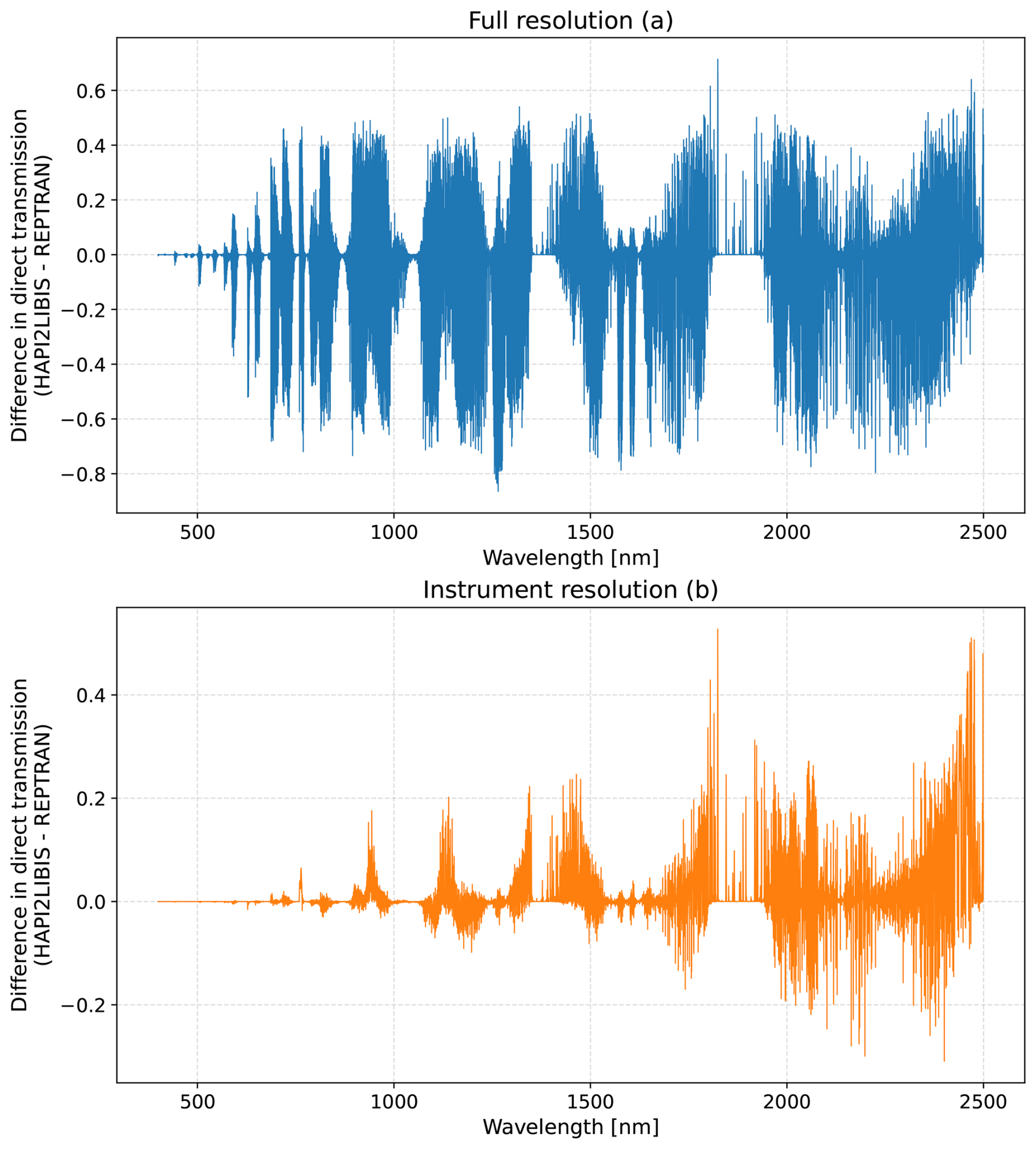
Figure A1 Differences in terms of simulated direct transmissions from sun to surface at full (a) and instrument (b) resolution when utilizing HAPI2LIBIS-generated molecular absorption optical depth files and REPTRAN fine-molecular-absorption parameterization.

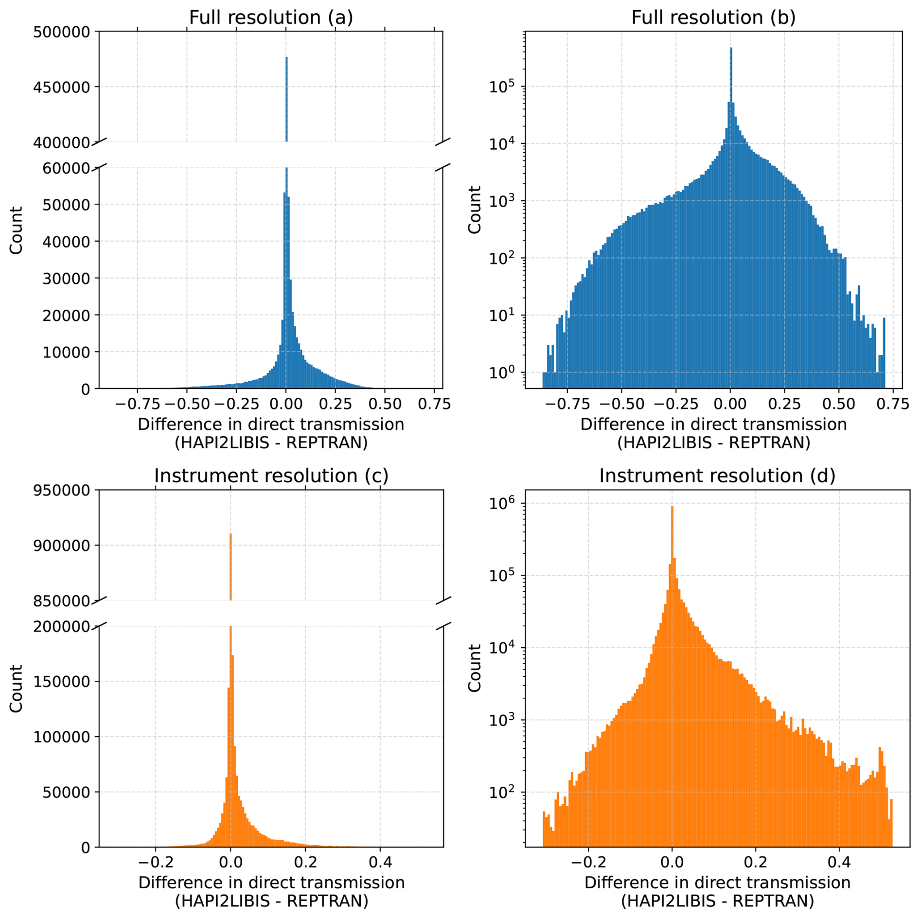
Figure A2 Histograms of the differences in terms of simulated direct transmissions from sun to surface at full (a–b) and instrument (c–d) resolution when utilizing HAPI2LIBIS-generated molecular absorption optical depth files and REPTRAN fine-molecular-absorption parameterization. For visual clarity, the vertical axis in panels (a) and (c) is cut.

Figure A3 Examples of optical thicknesses computed at different altitudes of the atmosphere by HAPI2LIBIS in the thermal-infrared wavelength region. Similarly to Fig. 5, contributions of CO₂ and H₂O are aggregated together.