Ensemble data assimilation to diagnose AI-based weather prediction models: a case with ClimaX version 0.3.1

Artificial intelligence (AI)-based weather prediction research is growing rapidly and has shown to be competitive with advanced dynamic numerical weather prediction (NWP) models. However, research combining AI-based weather prediction models with data assimilation remains limited, partially because long-term sequential data assimilation cycles are required to evaluate data assimilation systems. This study proposes using ensemble data assimilation for diagnosing AI-based weather prediction models and marked the first successful implementation of the ensemble Kalman filter with AI-based weather prediction models. Our experiments with an AI-based model, ClimaX, demonstrated that the ensemble data assimilation cycled stably for the AI-based weather prediction model using covariance inflation and localization techniques within the ensemble Kalman filter. While ClimaX showed some limitations in capturing flow-dependent error covariance compared to dynamical models, the AI-based ensemble forecasts provided reasonable and beneficial error covariance in sparsely observed regions. In addition, ensemble data assimilation revealed that error growth based on ensemble ClimaX predictions was weaker than that of dynamical NWP models, leading to higher inflation factors. A series of experiments demonstrated that ensemble data assimilation can be used to diagnose properties of AI weather prediction models, such as physical consistency and accurate error growth representation.

1 Introduction

The intensification of weather-induced disasters due to climate change is becoming increasingly severe worldwide (e.g., Jonkman et al., 2024). In a recent risk report, the World Economic Forum (2023) indicated that extreme weather is among the most severe global threats. To address extreme-weather events such as torrential heavy rains and heat waves, further advancements in weather forecasting are essential. There are two essential components for accurate weather forecasting: (1) numerical weather prediction (NWP) models that forecast future weather based on initial conditions and (2) data assimilation, which integrates atmospheric observation data to estimate initial conditions for subsequent forecasts by NWP models.

Since NVIDIA issued the first artificial intelligence (AI) weather prediction model, FourCastNet, which was competitive with dynamical NWP models, in February 2022 (Pathak et al., 2022; Bonev et al., 2023), deep-learning-based weather prediction research has shown rapid growth. A number of AI weather prediction models have been proposed, mainly by private information and technology (IT) companies, such as GraphCast by Google DeepMind (Lam et al., 2023), Pangu-Weather by Huawei (Bi et al., 2023), ClimaX and Stormer by Microsoft (Nguyen et al., 2023), and Aurora by Microsoft (Bodnar et al., 2025). These machine learning approaches have been shown to be competitive with state-of-the-art NWP models (e.g., Kochkov et al., 2024). Progress in AI-based weather prediction has been supported by the expansion of benchmark data and evaluation algorithms, such as WeatherBench (Rasp et al., 2020, 2024). Notably, most AI-based weather prediction models, including Pang-Weather, ClimaX, Stormer, and FourCastNet, use the Vision Transformer (ViT) neural network architecture (Vaswani et al., 2017; Dosovitskiy et al., 2021). The ViT, which has been explored in language models and image classifications, has been demonstrated to be effective in weather prediction as well.

However, research that couples AI-based weather prediction models with data assimilation remains limited. This limitation is partially due to the fact that long-term sequential data assimilation experiments are needed for the evaluation of data assimilation systems, in contrast to weather prediction tasks that allow for parallel learning using benchmark data. Conventional data assimilation methods used in NWP systems can be categorized into three groups: variational methods, ensemble Kalman filters, and particle filters. There are strong mathematical similarities between neural networks and variational data assimilation, both of which minimize their cost functions using their differentiable models. Because auto-differentiation codes are always available for neural-network-based AI models, AI weather prediction models are considered compatible with variational data assimilation methods, as in Xiao et al. (2024) and Adrian et al. (2025). On the other hand, recent studies have started to solve the inverse problem inherent in data assimilation using deep neural networks (McCabe and Brown, 2021; Chen et al., 2024; Bocquet et al., 2024; Luk et al., 2024; Vaughan et al., 2024). Some studies have employed ensemble Kalman filters for data-driven models (Hamilton et al., 2016; Penny et al., 2022; Chattopadhyay et al., 2022, 2023). However, no study has succeeded in employing ensemble Kalman filtering with global AI models of the atmosphere. Since AI models require significantly lower computational costs compared to dynamical NWP models, AI models offer benefits for ensemble-based methods, such as ensemble Kalman filters (EnKFs) and particle filters. Ensemble data assimilation at the global scale also allows us to assess the capability of data assimilation with AI models to handle spatially inhomogeneous observation networks and to maintain physically consistent multivariate error covariance across the entire atmosphere.

This study proposes using ensemble data assimilation for diagnosing AI-based weather prediction models. For that purpose, this study marks the first successful implementation of ensemble Kalman filter experiments with an AI weather prediction model to the best of the authors' knowledge. We applied the ViT-based ClimaX (Nguyen et al., 2023) to data assimilation experiments using the available source code and experimental environments with necessary modifications. For data assimilation, we applied the local ensemble transform Kalman filter (LETKF) (Hunt et al., 2007), which is among the most widely used data assimilation methods in operational NWP centers, such as the European Centre for Medium-Range Weather Forecasts (ECMWF), the Deutscher Wetterdienst (DWD), and the Japan Meteorological Agency (JMA). Using the coupled ClimaX–LETKF data assimilation system, we investigated several key aspects of AI-based weather prediction models, including whether the data assimilation cycles stably for the ClimaX AI weather prediction model using ensemble Kalman filters and whether AI-based ensemble weather prediction accurately represents flow-dependent background error variance and covariance. We also investigated whether techniques such as covariance inflation and localization, which are conventionally used in EnKFs for dynamical NWP models, are effective for AI weather prediction models. By addressing these research questions, we aim to advance the integration of AI weather prediction models with data assimilation techniques toward the development of more accurate weather forecasting. While this study primarily aims to use ensemble data assimilation for diagnosing AI-based weather prediction models, our research also represents an important step toward enabling real-time updates of AI weather models with meteorological observations.

The rest of the paper is organized as follows. Sect. 2 describes the methods and experiments, and Sect. 3 presents the results. Finally, Sect. 4 provides a discussion and summary.

2 Methods and experiments

2.1 ClimaX model

ClimaX (Nguyen et al., 2023) is a ViT-based AI weather prediction model for the global atmosphere. Variable tokenization and variable aggregation are key components of the ClimaX architecture on ViT, as they provide flexibility and generality. This study used the low-resolution version of ClimaX (version 0.3.1), with 64 and 32 zonal and meridional grid points, respectively, corresponding to a spatial resolution of 5.625° × 5.625°. The vertical model level was set at seven (900, 850, 700, 600, 500, 250, and 50 hPa).

By default, ClimaX is set to be trained against only five variables: geopotential at 500 hPa, temperature at 850 hPa, temperature at 2 m, zonal wind at 10 m, and meridional wind at 10 m. We updated ClimaX for data assimilation, which allowed the AI model to produce variables required for subsequent forecasts (Table 1). The updated ClimaX has state vectors, including zonal wind, meridional wind, temperature, specific humidity, and geopotential at seven vertical layers along with three surface variables: 10 m zonal wind, 10 m meridional wind, and 2 m temperature. We also diagnosed surface pressure, which is a required input for data assimilation, based on geopotential and surface elevation. Figure 1 shows the training curves of the default and updated ClimaX models verified against WeatherBench data (Rasp et al., 2020). Data for the period 2006–2015 were used for training, and data for 2016 were used for validation. Here we re-trained ClimaX entirely with the additional outputs (i.e., no transfer learning). It took approximately 4 h with four GPUs of NVIDIA RTX 6000Ada. Anomaly correlation coefficients increased, and root mean square errors (RMSEs) decreased, as shown in Fig. 1, indicating successful training of the updated ClimaX model. Because more variables were predicted by the updated ClimaX than by the default ClimaX, more training steps were required.

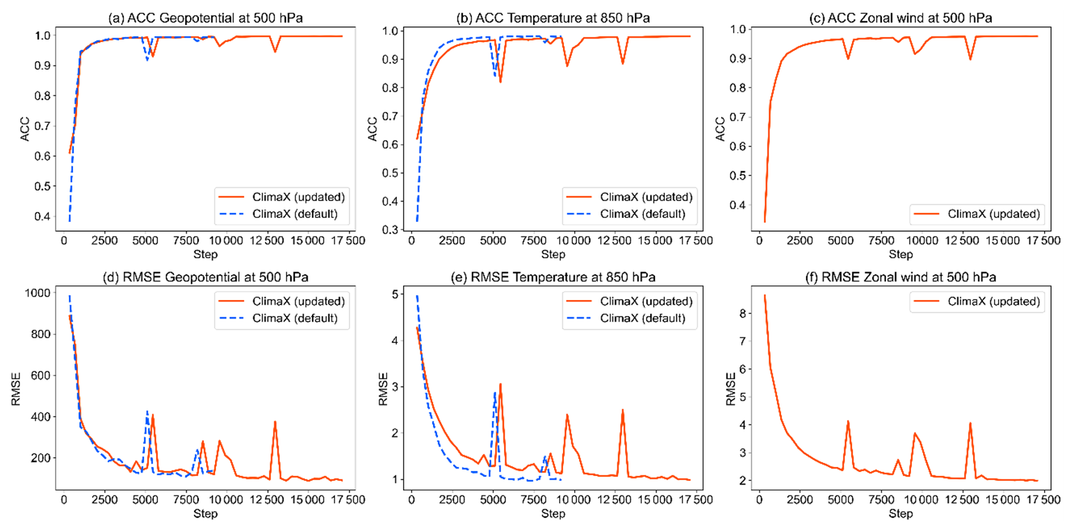
Figure 1 Training curves for the default and updated ClimaX models (dashed blue and solid orange lines) verified against WeatherBench data in 2016, as a function of the number of training steps. Each training step includes 64 training data in a mini batch. Panels (a)–(c) and (d)–(f) show anomaly correlation coefficients (ACCs) and root mean square errors (RMSEs). Panels (a) and (d), (b) and (e), and (c) and (f) are geopotential at 500 hPa (m² s⁻²), temperature at 850 hPa, and zonal wind at 500 hPa. There are no dashed blue lines in panels (c) and (f) because the default ClimaX model does not predict zonal wind at 500 hPa.

Table 1 Variables of the ClimaX model used in this study. ClimaX requires input variables to predict output variables. Observation (Obs) variables are assimilated with the associated error standard deviation (error SD).

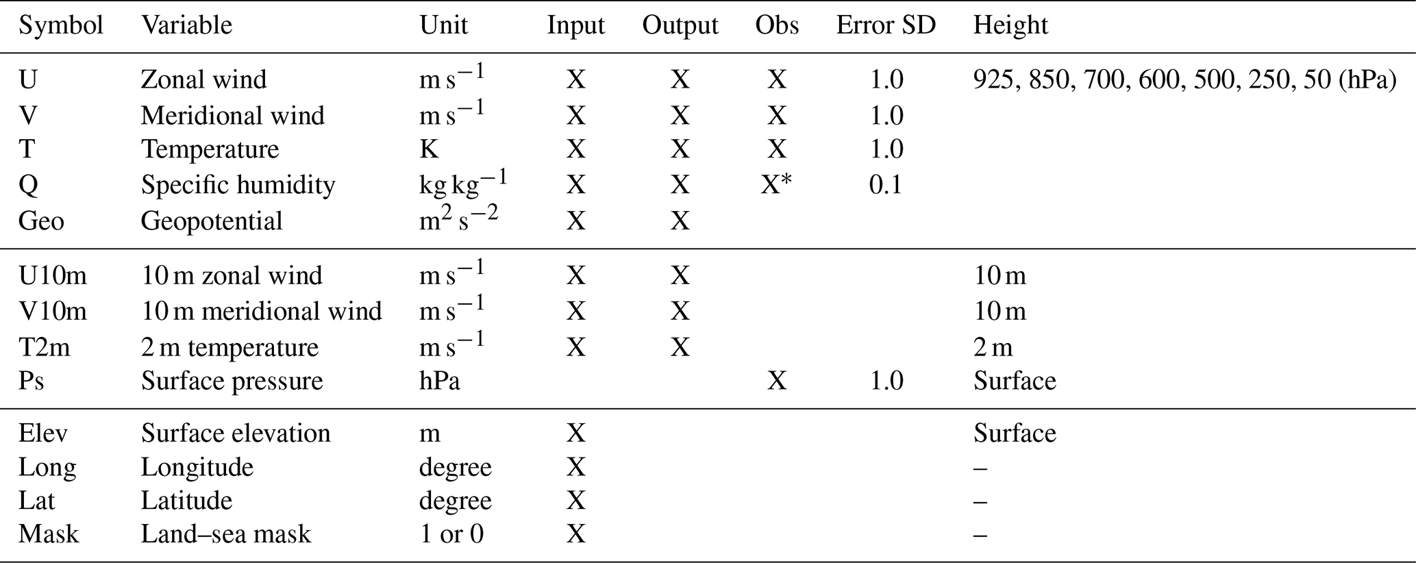
^* Specific humidity is observed up to the fourth model level (i.e., 925, 850, 700, and 600 hPa).

2.2 Local ensemble transform Kalman filter (LETKF)

The LETKF is among the most widely used data assimilation methods in operational NWP centers, such as ECMWF, DWD, and JMA. The LETKF simultaneously computes analysis equations at every model grid point with the assimilation of surrounding observations within the localization cut-off radius. The ClimaX–LETKF system was developed based on the SPEEDY–LETKF system (Kotsuki et al., 2022) by replacing the SPEEDY weather prediction model with ClimaX. Our future research can readily be expanded to particle filter experiments because the Kotsuki et al. (2022) system includes local particle filters in addition to the LETKF.

Let ${\mathbf{X}}_t\equiv \left\{{\mathit{x}}_t^{\left(\mathrm{1}\right)},\mathrm{\dots },{\mathit{x}}_t^{\left(m\right)}\right\}$ be an ensemble state matrix, whose ensemble mean and perturbation are given by ${\stackrel{\mathrm{‾}}{x}}_t$ (∈ℝⁿ) and $\mathit{\delta }{\mathbf{X}}_t\equiv \left\{{\mathit{x}}_t^{\left(\mathrm{1}\right)}-{\stackrel{\mathrm{‾}}{\mathit{x}}}_t,\mathrm{\dots },{\mathit{x}}_t^{\left(m\right)}-{\stackrel{\mathrm{‾}}{\mathit{x}}}_t\right\}$ ($\in {\mathbb{R}}^{n\times m}$), respectively. Here, n and m are the system and ensemble sizes. The superscript (i) and subscript t denote the ith ensemble member and the time, respectively. The EnKF, including LETKF, estimates the error covariance P ($\in {\mathbb{R}}^{n\times n}$) according to sample estimates based on ensemble perturbation:

$$\begin{array}{}\text{(1)}& \mathbf{P}\approx {\displaystyle \frac{\mathrm{1}}{m-\mathrm{1}}}\mathit{\delta }\mathbf{X}\mathit{\delta }{\mathbf{X}}^T.\end{array}$$

The analysis update equation of the LETKF is given by

$$\begin{array}{}\text{(2)}& {\displaystyle }\begin{array}{rl}{\mathbf{X}}_t^{\mathrm{a}}& ={\stackrel{\mathrm{‾}}{\mathit{x}}}_t^{\mathrm{b}}\cdot \mathbf{1}+\mathit{\delta }{\mathbf{X}}_t^{\mathrm{b}}{\stackrel{\mathrm{̃}}{\mathbf{P}}}_t^{\mathrm{a}}{\left({\mathbf{Y}}_t^{\mathrm{b}}\right)}^T{\mathbf{R}}_t^{-\mathrm{1}}\left({\mathit{y}}_t^{\mathrm{o}}-\stackrel{\mathrm{‾}}{H_t\left({\mathbf{X}}_t^{\mathrm{b}}\right)}\right)\\ & \cdot \mathbf{1}+{\left[\left(m-\mathrm{1}\right){\stackrel{\mathrm{̃}}{\mathbf{P}}}_t^{\mathrm{a}}\right]}^{\mathrm{1}/\mathrm{2}},\end{array}\text{(3)}& {\displaystyle }{\stackrel{\mathrm{̃}}{\mathbf{P}}}_t^{\mathrm{a}}={\left[{\displaystyle \frac{\left(m-\mathrm{1}\right)}{\mathit{\beta }}}\mathbf{I}+{\left({\mathbf{Y}}_t^{\mathrm{b}}\right)}^T{\mathbf{R}}_t^{-\mathrm{1}}{\mathbf{Y}}_t^{\mathrm{b}}\right]}^{-\mathrm{1}},\end{array}$$

where $\stackrel{\mathrm{̃}}{\mathbf{P}}$ is the error covariance matrix in the ensemble space ($\in {\mathbb{R}}^{m\times m}$), Y≡HδX is the ensemble perturbation matrix in the observation space ($\in {\mathbb{R}}^{p\times m}$), R is the observation error covariance matrix ($\in {\mathbb{R}}^{p\times p}$), y is the observation vector (∈ℝ^p), H is the observation operator that may be nonlinear, H ($\in {\mathbb{R}}^{p\times n}$) is the Jacobian of the linear observation operator matrix, and 1 is a row vector whose elements are all 1 (∈ℝ^m). Here, p is the number of observations. The superscripts o, b, and a denote the observation, background, and analysis, respectively. The scalar β is a multiplicative inflation factor which inflates the background error covariance such that ${\mathbf{P}}_t^{\mathrm{b}}\to \left(\mathrm{1}+\mathit{\beta }\right){\mathbf{P}}_t^{\mathrm{b}}$. This study uses the Miyoshi (2011) approach, which estimates spatially varying inflation factors adaptively based on observation–space statistics (Desroziers et al., 2005).

Localization is a practically important technique for EnKFs to eliminate long-range erroneous correlations due to the sample estimates of P with a limited ensemble size (Houtekamer and Zhang, 2016). Although a larger localization can spread observation data information for grid points distant from observations, a larger localization scale can yield suboptimal error covariance because of sampling errors. The LETKF inflates the observation error variance to realize the localization (Hunt et al., 2007) whose function is given by

$$\begin{array}{}\text{(4)}& \begin{array}{rl}& l=\\ & \left\{\begin{array}{l}\exp \left[-\frac{\mathrm{1}}{\mathrm{2}}\left\{{\left(d_{\mathrm{h}}/L_{\mathrm{h}}\right)}^{\mathrm{2}}+{\left(d_{\mathrm{v}}/L_{\mathrm{v}}\right)}^{\mathrm{2}}\right\}\right]\text{if}{d}_{\mathrm{h}}<\mathrm{2}\sqrt{\mathrm{10}/\mathrm{3}}{L}_{\mathrm{h}}\text{and}{d}_{\mathrm{v}}<\mathrm{2}\sqrt{\mathrm{10}/\mathrm{3}}{L}_{\mathrm{v}}\\ \mathrm{0}\text{else}\end{array},\right.\end{array}\end{array}$$

where l is the localization function, and its inverse l⁻¹ is multiplied to inflate R for the localization. Horizontal and vertical distances (km and log(Pa)) from the analysis grid point to the observation are defined by d_h and d_v, where subscripts h and v denote horizontal and vertical, respectively. Here, L_h and L_v are tunable horizontal and vertical localization scales (km and log(Pa)). The vertical localization scale L_v was set at 1.0 (log Pa) following the method of Kotsuki et al. (2022). Sensitivity to the horizontal localization scale for L_h= 400, 500, 600, 700, and 800 km is investigated in subsequent experiments.

2.3 Data assimilation experiments

In this study, all experiments were conducted as simulation experiments by generating observation data from WeatherBench with additions of Gaussian random noises. Although the real observation data were not directly assimilated, the assimilated observations reflect the real atmosphere in this study, in contrast to observing system simulation experiments. To approximate real-world scenarios, we considered radiosonde-like observations to generate atmospheric observation profiles for observing stations (Fig. 2). At observing stations, temperature and zonal and meridional winds were observed at all seven layers, whereas specific humidity was observed at the first to fourth layers. Table 1 shows the standard deviations of the observation errors. The network of observing stations and observation error standard deviations were consistent with those of the SPEEDY–LETKF experiments (Kotsuki et al., 2022; Kotsuki and Bishop, 2022). Observation data were produced at 6 h intervals such that the data assimilation interval was also 6 h. Since the observation data were generated directly at the model grid points, the observation operator is a linear operator composed only of 0.0 and 1.0.

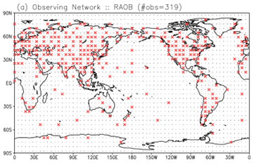
Figure 2 The observing network. The small black dots and red crosses represent model grid points and observing points, respectively.

We employed a series of data assimilation experiments over the year 2017, which is not used for training and validation of ClimaX. The ensemble size is 20. Their initial conditions for 00:00 UTC, 1 January 2017, were taken from WeatherBench data in 2006, which were sampled every 12 h from 00:00 UTC, 1 January 2006. Data assimilation experimental results were verified against WeatherBench data.

It should be noted that we were unable to conduct observation system simulation experiments (OSSEs), which require a natural run by ClimaX. This is because ClimaX could not produce long-term forecasts within our experimental configurations. A typical example is shown in Fig. 3. The forecasted temperature fields of ClimaX eventually began to deviate from the WeatherBench data with the continuation of 6 h forecasts. Ultimately, ClimaX produced meteorologically unrealistic weather fields, as demonstrated by the very low temperatures in the Pacific Ocean. Because AI models cannot learn physical laws in the absence of specific treatments, they are more likely to produce unrealistic weather fields under previously unencountered weather conditions. In other words, this suggests that ClimaX is unable to return to a meteorologically plausible attractor (or trajectory), while data assimilation enables ClimaX to synchronize with the real atmosphere, as shown in Sect. 3. This property in AI models was theoretically demonstrated by Adrian et al. (2025), who showed that long-term filter accuracy can be achieved with surrogate models if the models can provide accurate short-term forecasts. Applying neural networks that are informed or constrained by physical laws would be necessary to conduct observation system simulation experiments for AI-based weather prediction models.

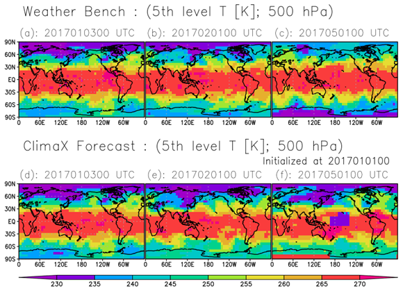
Figure 3 Spatial patterns of temperature (K) at the fifth model level (500 hPa). Panels (a)–(c) are WeatherBench data. Panels (d)–(f) are forecasts by ClimaX initialized at 00:00 UTC on 1 January 2017. Panels (a) and (d) show 00:00 UTC on 3 January 2017, (b) and (e) show 00:00 UTC on 1 February 2017, and (c) and (f) show 00:00 UTC on 1 May 2017.

3 Results

Figure 4 presents the time series of global mean root mean square errors (RMSEs) for temperature and geopotential height at the fifth model level, with four different horizontal localization scales (L_h). After the initiation of data assimilation, all experiments showed reductions in analysis errors. Experiments with L_h= 500, 600, and 700 km showed stable performance over a period of 1 year, until the end of 2017. Notably, data assimilation improved not only the observed variable, temperature, but also the unobserved variables, such as geopotential height. This indicates that observation information was propagated to unobserved variables through the data assimilation cycle. In contrast, the experiment with L_h= 800 km exhibited filter divergence after September 2017 due to erroneous error covariance associated with the larger localization scale. In addition, the experiment with L_h= 400 km kept reducing the RMSEs over a year, but the RMSEs were still higher than those of the other experiments, with the exception of L_h= 800 km. This indicates that a localization scale that is too small is suboptimal. This implies that ensemble-based error covariance is beneficial to some extent for propagating the impacts of assimilated observations for distant grid points.

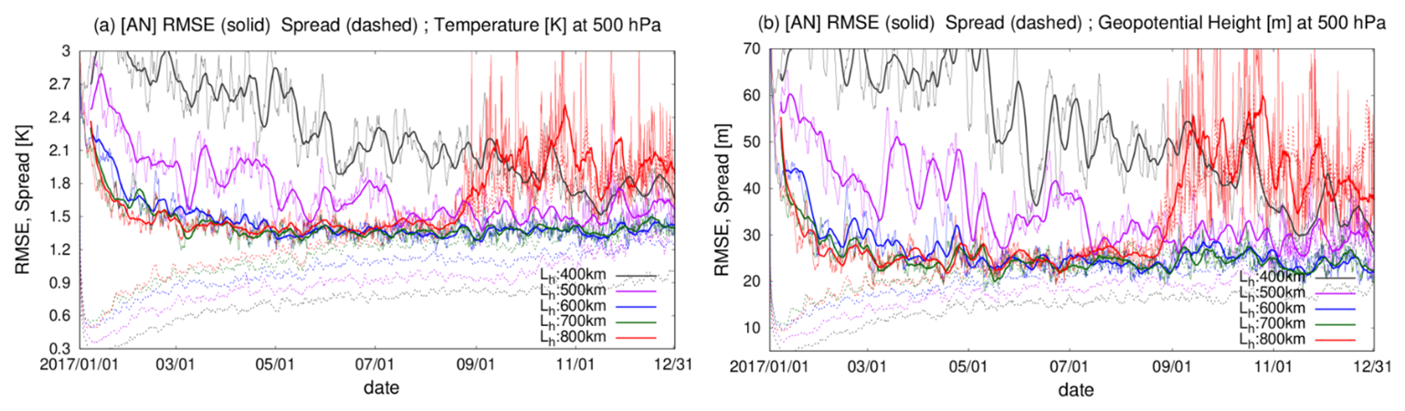
Figure 4 Time series of global mean root mean square errors (RMSEs) verified against WeatherBench data and ensemble spreads for (a) temperature (K) and geopotential height (m) at the fifth model level (500 hPa). The thin and bold solid lines indicate 6-hourly RMSEs and their 7 d running means, respectively. The dashed lines indicate ensemble spreads. The black, purple, blue, green, and red lines indicate the ClimaX–LETKF experiments at localization scales of L_h= 400, 500, 600, 700, and 800 km. The x axis indicates the date (month/day) in 2017.

Figure 5 shows the global mean RMSEs for zonal wind, meridional wind, temperature, specific humidity, geopotential height, and surface pressure as a function of the horizontal localization scales averaged over July–December 2017. At smaller localization scales (L_h= 400 and 500 km), the analysis RMSEs tended to be lower than the first-guess RMSEs, which suggests that data assimilation was beneficial in reducing errors. Conversely, at larger localization scales (L_h= 800 km), analysis RMSEs tended to be higher than the first-guess RMSEs, indicating that data assimilation degraded the analysis, presumably also due to excessive error covariance at larger localization scales. In addition, the analysis RMSEs were slightly higher than the first-guess RMSEs for some variables at L_h= 700 km, although the data assimilation cycled stably (Fig. 4). In general, stable filters are expected to yield overall RMSE reduction unless the system is non-chaotic. Therefore, these results for L_h= 700 km imply that the present ClimaX exhibits weaker chaotic behavior compared to the real atmosphere.

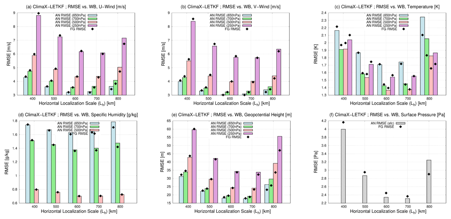
Figure 5 Global mean root mean square errors (RMSEs) verified against WeatherBench (WB) for (a) zonal wind (m s⁻¹), (b) meridional wind (m s⁻¹), (c) temperature (K), (d) specific humidity (g kg⁻¹), (e) geopotential height (m), and (f) surface pressure (hPa) as a function of the horizontal localization scales (km) averaged over July–December 2017. The colored bars and black diamonds indicate analysis (AN) and first-guess (FG) RMSEs, respectively. The blue, green, red, and purple bars in panels (a)–(e) represent the second, third, fifth, and sixth model levels (850, 700, 500, and 250 hPa, respectively). The gray bars in panel (f) represent surface pressure. The RMSEs of specific humidity at the sixth model level in panel (d) were too low to be shown.

Among the five experiments, a localization scale of L_h= 600 km yielded the lowest analysis RMSEs for most variables. Significant analysis error reductions were observed for temperature and surface pressure. However, no clear impacts were observed for zonal and meridional winds. Even slight degradations were detected, implying that spatial and inter-variable error covariance may not be well represented in our ClimaX–LETKF.

Here, we investigate the spatial patterns of the difference between the analysis and first-guess mean absolute errors, which is given by

$$\begin{array}{}\text{(5)}& {\mathrm{MAE}}_{\mathrm{diff}}={\displaystyle \frac{\mathrm{1}}{N_t}}{\sum }_t\left|{\stackrel{\mathrm{‾}}{\mathit{x}}}_t^{\mathrm{a}}-{\mathit{x}}_t^{\mathrm{WB}}\right|-\mathrm{|}{\stackrel{\mathrm{‾}}{\mathit{x}}}_t^{\mathrm{b}}-{\mathit{x}}_t^{\mathrm{WB}}\mathrm{|},\end{array}$$

where N_t is the sample size, and superscript WB represents WeatherBench data. Negative and positive values indicate improvements and degradations due to data assimilation. Figure 6 shows the MAE_diff for four variables (zonal wind at 850 hPa, temperature at 700 hPa, geopotential height at 500 hPa, and surface pressure) based on the experiments with the localization scale L_h= 500 km, which resulted in RMSE reductions by data assimilation for most of the variables in Fig. 5. General improvements are seen at grid points with observations for zonal wind and temperature (Fig. 6a and b). However, there were also slight degradations at grid points surrounding observing stations, such as those in the Arctic Ocean and along the US and Japanese coasts. We also see degradations for geopotential height, where temperature and zonal wind degradations are presented (Fig. 6c). These degradations suggest that ensemble-based spatial error covariance was suboptimal in these regions. In contrast, geopotential height and surface pressure generally improved in the Southern Hemisphere (Fig. 6c and d). In particular, improvements are seen even at grid points surrounding observing stations in the Southern Hemisphere. Specifically, using the spatial and inter-variable error covariance based on AI ensemble forecasts was advantageous for geopotential heights and surface pressure in sparsely observed regions.

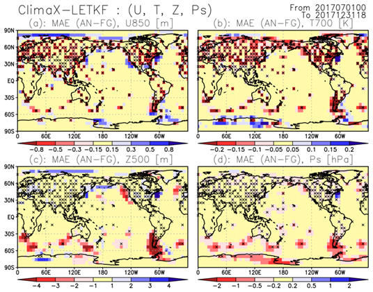
Figure 6 Spatial patterns of difference between analysis (AN) and first-guess (FG) mean absolute errors (MAEs) for (a) zonal wind (m s⁻¹) at 850 hPa, (b) temperature (K) at 700 hPa, (c) geopotential height (m) at 500 hPa, and surface pressure (hPa), averaged over July–December 2017. The warm and cold colors represent improvements and degradations due to data assimilation. Results are for a localization scale of L_h= 500 km. The black crosses indicate observing stations.

Another important property is that ClimaX would be less chaotic than dynamical NWP models, as indicated by the estimated inflation factor β diagnosed by observation–space statistics (Fig. 7). In addition, the larger inflation would also indicate greater model error in ClimaX, which requires stronger inflation to account for the model's imperfection. Compared to our study, Kotsuki et al. (2017) estimated a much smaller inflation factor for a global ensemble data assimilation system using a dynamical model (see Fig. 10a in Kotsuki et al., 2017). For example, the inflation factors in Kotsuki et al. (2017) were at most around 2.0, whereas ClimaX–LETKF required inflation factors exceeding 5.0. Selz and Craig (2023) noted that an AI-based weather prediction model failed to reproduce rapid initial error growth rates, which would prevent it from replicating the butterfly effect as accurately as dynamical NWP models.

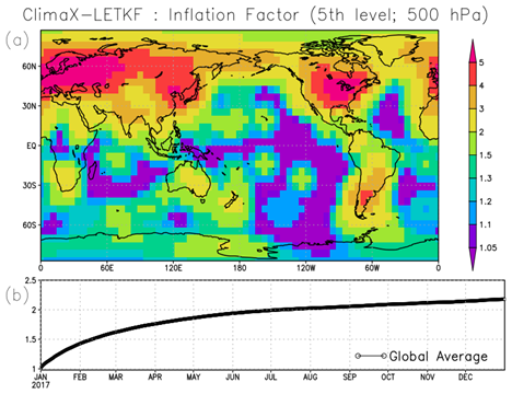
Figure 7 (a) Spatial pattern of the multiplicative inflation factor at the end of the experiment on 18:00 UTC of 31 December 2017. (b) Time series of globally averaged inflation factors. Results are for a localization scale of L_h= 600 km.

4 Discussion and summary

The optimal localization scale was unexpectedly very small in Fig. 5. Kondo and Miyoshi (2016) pointed out that a larger localization scale is beneficial for low-resolution models and larger ensemble sizes (see Table 1 in Kondo and Miyoshi, 2016). Our optimal localization scale for the 20-member ClimaX–LETKF was 600 km, which is shorter than the 700–900 km scale of the 20-member LETKF experiments coupled with a dynamical NWP model (also known as SPEEDY; Molteni, 2003) (e.g., Miyoshi and Kondo, 2013, Fig. 2b in Kotsuki and Bishop, 2022). Nevertheless, considering that the SPEEDY model has a finer horizontal resolution (96 × 48 horizontal grids) than ClimaX used in this study (64 × 32 horizontal grids), it remains plausible that ClimaX captures flow-dependent error covariance less effectively than dynamical NWP models. Bonavita (2024) investigated physical realism of the present AI models (FourCastNet, Pangu-Weather, and GraphCast) and concluded that AI models are not able to properly reproduce sub-synoptic and mesoscale weather phenomena. The suboptimal flow-dependent error covariance in this study can be attributed to physically inconsistent atmospheric fields of the ClimaX predictions.

Two major advancements are required for AI-based weather prediction models to improve ensemble data assimilation. First, it is imperative that AI models generate physically consistent forecast variables. The accuracy of spatial and inter-variable error covariance would be improved by this enhancement, which would require AI model training procedures to include physical constraints such as hydrostatic and geostrophic balances, in addition to decreasing the mean square errors of the target variables. Second, it is crucial to accurately capture the error growth rate. Our findings demonstrated that error growth based on ensemble ClimaX predictions was weaker than that of dynamical NWP models, leading to higher inflation factors (Fig. 7). Thus, ensemble forecasts produced by AI weather prediction models likely exhibit insufficient spread. In weather forecasting, capturing forecast uncertainty is as important as providing accurate forecasts. Recent studies have begun to develop models for generating statistically accurate ensembles by using generative models (Price et al., 2025) or by training on probabilistic cost functions (Kochkov et al., 2024). Other possible solutions for improving the error growth are to develop a set of slightly different AI models by randomizing the seed in the AI training process as an analogy to stochastic parameterization (Weyn et al., 2021) or to incorporate the Lyapunov exponent within the cost function of model training (Platt et al., 2023). Note that the present experiments were conducted at a coarse resolution of 5.625°, which may limit the ability of the ClimaX–LETKF system to accurately diagnose localized weather phenomena. At higher spatial resolutions, AI models may capture mesoscale and sub-synoptic features, potentially leading to more realistic ensemble-based error covariances. Future work will explore the data assimilation system's behaviors at higher resolutions using more advanced versions of AI models with denser observation datasets.

Despite the need for further improvements, this study represents a significant step toward ensemble data assimilation for AI-based weather prediction models. Notably, we demonstrated that the data assimilation cycled stably for the AI-based weather prediction model ClimaX with the LETKF using covariance inflation and localization techniques. In addition, the ensemble-based error covariance was estimated reasonably well by the AI-based weather prediction model in sparsely observed regions.

Additional research is anticipated for areas identified as requiring further improvements. For that purpose, ensemble data assimilation is a useful tool for diagnosing AI-based weather forecasting models. That is, investigating optimal localization scales, ensemble-based error covariance, and necessary inflation factors gives beneficial insights into understanding the properties of AI models. After achieving these two major advancements, it is important to employ a systematic sensitivity analysis for the localization radius and ensemble size. A suitable inflation method for AI-based weather prediction models also remains to be explored. Comparing the EnKF with variational or ensemble–variational approaches would be an important topic for future investigation. Since AI models require much lower computational costs compared to dynamical NWP models, extending the present study to large-ensemble EnKFs or a local particle filter (LPF) is also an important subject of future studies. Our future work will investigate the applicability of the proposed system to real-time forecasting with higher-resolution AI models with real weather observations, such as PREPBUFR and satellite radiances. The analysis fields and ensemble spreads generated by the ensemble data assimilation with assimilation of real observations may be applicable to subsequent training of AI models. Most current AI weather models are trained on reanalysis data such as WeatherBench, without explicitly accounting for the uncertainty in analysis (i.e., analysis ensemble spread). By using ensemble spreads or individual ensemble members, the training process of AI models could be improved, such as by relaxing penalties in regions with large ensemble spread.

Beyond weather prediction, data assimilation has been successfully combined with machine-learning-based surrogate models in various fields, including oceanography, hydrology, and wildfire (e.g., Brajard et al., 2021; Cheng et al., 2022; Jeong et al., 2024). It would be beneficial to explore how the EnKF could be applied to diagnose AI-based models in other fields.