The discontinuous Galerkin coastal and estuarine modelling system (DGCEMS v1.0.0): a three-dimensional, nonsplit-mode, implicit–explicit Runge–Kutta hydrostatic model

Numerical methods of discontinuous Galerkin (DG) discretisation for coastal ocean modelling have advanced significantly, but there are still challenges in accurately simulating phenomena such as wetting and drying processes and baroclinic flows in coastal and estuarine regions. This study develops a novel three-dimensional (3D) coastal and estuarine modelling system named DGCEMS, using a quadrature-free nodal DG method. The model adopts σ coordinates, employs a nonsplit-mode framework, and integrates a semi-implicit Runge–Kutta scheme. A series of numerical experiments demonstrate the model's second-order convergence, low spurious mixing, and capability to simulate salt–freshwater interactions in the presence of wetting and drying boundaries.

1 Introduction

During the past few decades, numerical methods have evolved dramatically, and coastal ocean models can benefit from these advanced numerical methods (Blaise et al., 2010). Classical three-dimensional (3D) hydrodynamic models, e.g. ROMS (Shchepetkin and McWilliams, 2005), Delft3D (Lesser et al., 2004), FVCOM (Chen et al., 2003), TELEMAC (Moulinec et al., 2011), and SCHISM (Zhang et al., 2016), can be utilised to predict storm surges, tsunamis, and floods and assess environmental qualities by adding additional equations (e.g. transport and reaction) to model oil slicks, contaminant plume propagation, temperature, and salinity transport, among other problems (Bertsch et al., 2022; Zhou et al., 2024; Sanz-Ramos et al., 2023).

In coastal and estuary waters, the presence of large gradients and strong discontinuity processes (e.g. wetting and drying processes and saline flow) may pose challenges for these classical circulation models, such as maintaining high numerical accuracy, minimising numerical mixing, and preventing excessive diffusion. From the perspective of numerical discretisation methods in the above models, the finite-volume (FV) method is known to have limitations in developing high-order accuracy schemes and incorporating so-called hp adaptivity (Lee, 2019). High-order FV models can increase the order by wide stencils, but they have to perform complex numerical reconstruction, which significantly increases computational complexity (Cheng et al., 2016). Models based on the finite-element (FE) method can also achieve high order, but they do not have local conservation. In the wet–dry (WD) fronts and in small-scale dynamics like baroclinic eddies, where local conservation of mass and momentum is critical, the property of local conservation is a preferred characteristic of a numerical scheme (Lee, 2020).

As a combination of both FV and FE methods, the discontinuous Galerkin (DG) method, with a relatively small number of elements, is well suited to modelling of 3D flows exhibiting strong velocity or density gradients. Dawson and Aizinger (2005) first developed a 3D shallow-water equation (SWE) model based on DG methods called UTBEST3D. They used z coordinates in a vertical direction and a local discontinuous Galerkin (LDG) method for vertical diffusion (Aizinger and Dawson, 2007). To reduce the degrees of stiffness, Blaise et al. (2010) and Comblen et al. (2010) developed a 3D baroclinic marine model called SLIM3D and used the symmetric interior penalty Galerkin method (SIPG) to discrete the vertical diffusion. In addition, the mode-splitting procedure, which splits the 2D external mode and the 3D internal mode, is used to save computational time (Kowalik and Murty, 1993). Later, Delandmeter et al. (2018) added a fully consistent and conservative vertically adaptive coordinate system in SLIM3D. At the same time, Kärnä et al. (2018) also developed a 3D DG baroclinic model called Thetis. Thetis includes a more accurate mode-splitting method, revised viscosity formulation, and new second-order time integration scheme, which has lower or comparable numerical dissipation. The above three models all choose z coordinates, considering that σ coordinates enable a smooth representation of the bottom topography, which is particularly appropriate for coastal applications. Using σ coordinates, Conroy and Kubatko (2016) explicitly treated the vertical diffusion term to study the water column concerning barotropic forcing by building a 3D DG SWE model. The model of Conroy and Kubatko (2016) does not consider nonlinear advective terms and can only investigate 3D linear problems. The mentioned models use the quadrature-based nodal DG method. In explicit and semi-implicit time stepping schemes commonly used in connection with the SWE models, the most computationally expensive parts of a DG algorithm are the element and edge integrals computed via loops over quadrature points (Faghih-Naini et al., 2020). One criticism of the original DG method is that it requires expensive quadrature rules to reduce the aliasing error arising in the nonlinear system. The essence of the quadrature-free approach is to convert the nonlinear fluxes to polynomials or polynomial operations, which can be integrated analytically into the element or element boundaries (Li, 2024). The quadrature-free DG scheme has a comparable order and L₂ errors even at the 7th order of accuracy compared to the quadrature-based DG scheme for the isentropic vortex problem (Nair, 2015). In the MATLAB–C hybrid framework, Ran et al. (2022) developed a 3D barotropic model based on the quadrature-free nodal DG method. They choose the nonsplit-mode scheme considering that this method does not need to adjust the differences in the momentum calculation between the 2D external mode and the 3D internal mode and has fewer excessive errors (Chen et al., 2022; Conroy and Kubatko, 2016). A series of numerical experiments have proven the accuracy and potential application value of the barotropic model, but its computational efficiency is low, which limits the applicability of the model.

In addition to the utilisation of different numerical discretisation schemes, wetting and drying (WD) processes should be included in coastal and estuarine modelling, which is a challenge for 3D DG models. At present, within existing 3D DG models, Vallaeys (2018) noted that the WD processes can be considered in the external mode of the mode-splitting SLIM3D model, but this kind of wetting and drying module cannot be operated together with the baroclinic module. Chen et al. (2024) developed a WD treatment in a 3D DG model with the nonsplit-mode scheme, but there is still no description and verification of the coexistence of WD processes and thermohaline transport.

To adapt to the complex terrain of estuary and coastal areas and have a comparable calculation accuracy to existing 3D DG baroclinic models, this work aims to develop a new share-code discontinuous Galerkin coastal and estuarine modelling system (DGCEMS) for a 3D nonsplit-mode, implicit–explicit Runge–Kutta baroclinic model using σ coordinates with a WD module based on a quadrature-free nodal DG scheme. The arrangement of this paper is as follows. Section 2 describes the model with the discretisation of each term in the model, while Sect. 3 presents numerical tests and applications to show the main functionality of the model. Conclusions are given in Sect. 4.

2 Model and discretisation

2.1 Governing equations

The conservative and pre-balanced scheme of 3D shallow-water equations in the σ coordinates, with advection–diffusion equations of temperature T and salinity S, can be written as

$$\begin{array}{}\text{(1)}& {\mathit{U}}_{\mathrm{t}}+\mathrm{\nabla }\cdot \mathit{F}\left(\mathit{U}\right)=\mathit{S}\left(\mathit{U}\right).\end{array}$$

Here $\mathit{U}=[D,Du,Dv,DT,DS{]}^{\mathrm{T}}$, where D is the water depth, and u and v are the velocity components along the x and y directions, respectively. The convective term $\mathit{F}\left(\mathit{U}\right)=\left[\mathit{E}\right(\mathit{U}),\mathit{G}(\mathit{U}),\mathit{H}(\mathit{U}\left)\right]$, and each part in this term can be written as

$$\begin{array}{}\text{(2)}& \begin{array}{rl}& \mathit{E}\left(\mathit{U}\right)=\left[\begin{array}{c}Du\\ D{u}^{\mathrm{2}}+\mathrm{1}/\mathrm{2}\left(g\left(D^{\mathrm{2}}-z_{\mathrm{b}}^{\mathrm{2}}\right)\right)\\ Duv\\ DuT\\ DuS\end{array}\right],\\ & \mathit{G}\left(\mathit{U}\right)=\left[\begin{array}{c}Dv\\ Duv\\ D{v}^{\mathrm{2}}+\mathrm{1}/\mathrm{2}\left(g\left(D^{\mathrm{2}}-z_{\mathrm{b}}^{\mathrm{2}}\right)\right)\\ DvT\\ DvS\end{array}\right],\mathit{H}\left(\mathit{U}\right)=\left[\begin{array}{c}\mathit{\omega }\\ \mathit{\omega }u\\ \mathit{\omega }v\\ \mathit{\omega }T\\ \mathit{\omega }S\end{array}\right],\end{array}\end{array}$$

where g is gravitational acceleration; z_b is the bottom elevation, and ω is the vertical velocity along the σ direction. The right side of Eq. (1) contains the terms of

$$\begin{array}{}\text{(3)}& \mathit{S}\left(\mathit{U}\right)={\mathit{S}}_{\mathrm{b}}+{\mathit{S}}_{\mathrm{f}}+{\mathit{S}}_{\mathrm{d},\mathrm{h}}+{\mathit{S}}_{\mathrm{d},\mathrm{v}}+{\mathit{S}}_{\text{baro}},\end{array}$$

where S_b, S_f, S_d,h, S_d,v, and S_baro represent the bottom topography term, Coriolis acceleration term, horizontal diffusion term, vertical diffusion term, and baroclinic term, respectively. The five terms are given as follows:

$$\begin{array}{}\text{(4)}& {\displaystyle }{\mathit{S}}_{\mathrm{b}}=\left[\begin{array}{c}\mathrm{0}\\ -g\mathit{\eta }\partial z_{\mathrm{b}}/\partial x\\ -g\mathit{\eta }\partial z_{\mathrm{b}}/\partial y\\ \mathrm{0}\\ \mathrm{0}\end{array}\right],{\mathit{S}}_{\mathrm{f}}=\left[\begin{array}{c}\mathrm{0}\\ -fDv\\ fDu\\ \mathrm{0}\\ \mathrm{0}\end{array}\right],\text{(5)}& {\displaystyle }\begin{array}{rl}& {\mathit{S}}_{\mathrm{d},\mathrm{h}}=\left[\begin{array}{c}\mathrm{0}\\ \frac{\partial }{\partial x}\left(K_{\mathrm{h}}D\frac{\partial u}{\partial x}\right)+\frac{\partial }{\partial y}\left(K_{\mathrm{h}}D\frac{\partial u}{\partial y}\right)\\ \frac{\partial }{\partial x}\left(K_{\mathrm{h}}D\frac{\partial v}{\partial x}\right)+\frac{\partial }{\partial y}\left(K_{\mathrm{h}}D\frac{\partial v}{\partial y}\right)\\ \frac{\partial }{\partial x}\left(K_{\mathrm{H}}D\frac{\partial T}{\partial x}\right)+\frac{\partial }{\partial y}\left(K_{\mathrm{H}}D\frac{\partial T}{\partial y}\right)\\ \frac{\partial }{\partial x}\left(K_{\mathrm{H}}D\frac{\partial S}{\partial x}\right)+\frac{\partial }{\partial y}\left(K_{\mathrm{H}}D\frac{\partial S}{\partial y}\right)\end{array}\right],\\ & {\mathit{S}}_{\mathrm{d},\mathrm{v}}=\left[\begin{array}{c}\mathrm{0}\\ \frac{\partial }{\partial \mathit{\sigma }}\left(\frac{K_{\mathrm{v}}}{D^{\mathrm{2}}}\frac{\partial Du}{\partial \mathit{\sigma }}\right)\\ \frac{\partial }{\partial \mathit{\sigma }}\left(\frac{K_{\mathrm{v}}}{D^{\mathrm{2}}}\frac{\partial Dv}{\partial \mathit{\sigma }}\right)\\ \frac{\partial }{\partial \mathit{\sigma }}\left(\frac{K_{\mathrm{V}}}{D^{\mathrm{2}}}\frac{\partial DT}{\partial \mathit{\sigma }}\right)\\ \frac{\partial }{\partial \mathit{\sigma }}\left(\frac{K_{\mathrm{V}}}{D^{\mathrm{2}}}\frac{\partial DS}{\partial \mathit{\sigma }}\right)\end{array}\right],\end{array}\text{(6)}& {\displaystyle }{\mathit{S}}_{\text{baro}}=\left[\begin{array}{c}\mathrm{0}\\ -\frac{gD}{{\mathit{\rho }}_{\mathrm{0}}}\left[{\int }_{\mathit{\sigma }}^{\mathrm{0}}D\frac{\partial \mathit{\rho }}{\partial x}\mathrm{d}\mathit{\sigma }-\frac{\partial D}{\partial x}{\int }_{\mathit{\sigma }}^{\mathrm{0}}\mathit{\sigma }\frac{\partial \mathit{\rho }}{\partial \mathit{\sigma }}\mathrm{d}\mathit{\sigma }\right]\\ -\frac{gD}{{\mathit{\rho }}_{\mathrm{0}}}\left[{\int }_{\mathit{\sigma }}^{\mathrm{0}}D\frac{\partial \mathit{\rho }}{\partial y}\mathrm{d}\mathit{\sigma }-\frac{\partial D}{\partial y}{\int }_{\mathit{\sigma }}^{\mathrm{0}}\mathit{\sigma }\frac{\partial \mathit{\rho }}{\partial \mathit{\sigma }}\mathrm{d}\mathit{\sigma }\right]\\ \mathrm{0}\\ \mathrm{0}\end{array}\right],\end{array}$$

where $\mathit{\eta }=D+z_{\mathrm{b}}$ is the surface elevation; f is the Coriolis coefficient; K_h and K_H are the horizontal (eddy) diffusion coefficients using Smagorinsky's method (Smagorinsky, 1963); K_v and K_V are the vertical (eddy) diffusion coefficients calculated by the MY-2.5 turbulent closure scheme in the General Ocean Turbulence Model (GOTM; Burchard et al., 1999); ρ₀ is the reference density; and the water density ρ is defined as $\mathit{\rho }=\mathit{\rho }(T,S)$, which is a function of T and S. In the model, two state equations can be chosen: linear, shown in Eq. (7), and full nonlinear, from Jackett et al. (2006):

$$\begin{array}{}\text{(7)}& \mathit{\rho }(T,S)={\mathit{\rho }}_{\mathrm{0}}-{\mathit{\alpha }}_{\mathrm{T}}(T-T_{\mathrm{0}})+{\mathit{\beta }}_{\mathrm{S}}(S-S_{\mathrm{0}}).\end{array}$$

In Eq. (7), α_T and β_S are coefficients. T₀ and S₀ are reference temperature and salinity, respectively. It can be seen that the above system has seven prognostic variables, namely D (or η)T, u, v, ω, ρ, T, and S, but there are a total of six equations (Eqs. 1 and 7) to be solved. To this end, the depth-averaged continuity equation is applied to calculate the water depth (or free surface) for the nonsplit-mode model, which can be written as

$$\begin{array}{}\text{(8)}& {\displaystyle \frac{\partial D}{\partial t}}+{\displaystyle \frac{\partial DU}{\partial x}}+{\displaystyle \frac{\partial DV}{\partial y}}=\mathrm{0},\end{array}$$

where $U={\int }_{-\mathrm{1}}^{\mathrm{0}}u\mathrm{d}\mathit{\sigma }$ and $V={\int }_{-\mathrm{1}}^{\mathrm{0}}v\mathrm{d}\mathit{\sigma }$ are depth-averaged horizontal velocities. The vertical velocity is solved by combining 2D and 3D continuity equations, which can be written as

$$\begin{array}{}\text{(9)}& {\displaystyle \frac{\partial \mathit{\omega }}{\partial \mathit{\sigma }}}={\displaystyle \frac{\partial (DU-Du)}{\partial x}}+{\displaystyle \frac{\partial (DV-Dv)}{\partial y}}\end{array}$$

and then be integrated layer by layer along the vertical direction.

2.2 Discontinuous Galerkin discretisation

In this section, we describe the numerical implementation of DGCEMS. The DG function spaces are defined in Sect. 2.2.1, followed by the quadrature-free nodal DG discretisation (Hesthaven and Warburton, 2007) of the above governing equations.

2.2.1 Function spaces and notations

For a 3D computational domain, Ω_3d, there is a corresponding projection at the horizontal plane, which is denoted as Ω_2d, and it can be divided by an unstructured triangular mesh. These triangular elements extend vertically and form triangular prisms, which are computational elements in Ω_3d. The DG discretisation of this model is based on the linear function space, which is denoted as $P_{N_{\mathrm{h}}}$ in the 2D space and $P_{(N_{\mathrm{h}},N_{\mathrm{v}})}$ in the 3D space (in Fig. 1, both N_h and N_v are equal to 1, representing the stage of the function of horizontal and vertical space). It should be noted that the number of vertical layers in the model is flexible and user-defined. The vertical discretisation shown in Fig. 1 employs two layers for illustrative purposes only, to demonstrate the distribution of interpolation nodes in the σ-coordinate direction. In practical simulations, more vertical layers (e.g. 10 to 20 layers) are typically used to improve the resolution of vertical velocity profiles and stratification. Increasing the number of layers enhances vertical accuracy but does not change the order of numerical convergence and may increase computational cost. We set ${\mathit{\varphi }}_{\mathrm{2}\mathrm{d}}\in P_{N_{\mathrm{h}}}$, ${\mathit{\phi }}_{\mathrm{2}\mathrm{d}}\in P_{N_{\mathrm{h}}}^{\mathrm{2}}$, ${\mathit{\varphi }}_{\mathrm{3}\mathrm{d}}\in P_{(N_{\mathrm{h}},N_{\mathrm{v}})}$, and ${\mathit{\phi }}_{\mathrm{3}\mathrm{d}}\in P_{(N_{\mathrm{h}},N_{\mathrm{v}})}^{\mathrm{2}}$ as the test functions in the 2D and 3D function spaces.

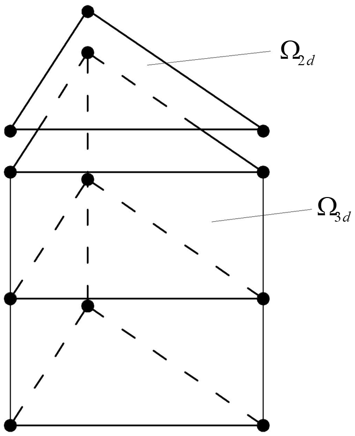
Figure 1 Schematic of vertical computational element distribution (example with two layers). Black dots represent the interpolation nodes corresponding to the horizontal first-order and vertical first-order basis functions.

Next, we use the following notations to represent the volume and surface integrals:

$$\begin{array}{}\text{(10)}& {\displaystyle }& {\displaystyle }\langle \cdot {\rangle }_{\mathrm{\Omega }}=\underset{\mathrm{\Omega }}{\int }(\cdot )\mathrm{d}\mathit{x},\text{(11)}& {\displaystyle }& {\displaystyle }\langle \langle \cdot \rangle {\rangle }_{\partial \mathrm{\Omega }}=\underset{\partial \mathrm{\Omega }}{\int }(\cdot )\mathrm{d}s.\end{array}$$

In surface terms, we additionally define the concept of the average, {{⋅}}, and the jump, [[⋅]], to simplify the expression of subsequent formulas:

$$\begin{array}{}\text{(12)}& {\displaystyle }& {\displaystyle }\mathit{\left\{}\mathit{\right\{}a\mathit{\left\}}\mathit{\right\}}={\displaystyle \frac{\mathrm{1}}{\mathrm{2}}}(a^{+}+a^{-}),\text{(13)}& {\displaystyle }& {\displaystyle }\mathit{\left\{}\mathit{\right\{}\mathit{b}\mathit{\left\}}\mathit{\right\}}={\displaystyle \frac{\mathrm{1}}{\mathrm{2}}}({\mathit{b}}^{+}+{\mathit{b}}^{-}),\text{(14)}& {\displaystyle }& {\displaystyle }\left[\left[a\mathit{b}\right]\right]=a^{+}{\mathit{b}}^{+}+a^{-}{\mathit{b}}^{-},\text{(15)}& {\displaystyle }& {\displaystyle }\left[\left[\mathit{b}\cdot n\right]\right]={\mathit{b}}^{+}\cdot {\mathit{n}}^{+}+{\mathit{b}}^{-}\cdot {\mathit{n}}^{-},\text{(16)}& {\displaystyle }& {\displaystyle }\left[\left[\mathit{b}\mathit{n}\right]\right]={\mathit{b}}^{+}{\mathit{n}}^{+}+{\mathit{b}}^{-}{\mathit{n}}^{-},\end{array}$$

where a represents a scalar field and b represents a vector field, − and + are the local side and adjacent side, and $n=(n_x,n_y,n_{\mathit{\sigma }})$ is the outward unit normal on the edges. Let 𝒯 and 𝒫 stand for the partition of the 2D domain Ω_2d and 3D domain Ω_3d, respectively. Element interfaces are denoted by ${\mathcal{I}}_{\mathrm{2}\mathrm{d}}=\mathit{\{}{k}_i\cap k_j\mathrm{|}{k}_i,k_j\in \mathcal{T},i\ne j\mathit{\}}$, while ℐ_h and ℐ_v are notations of horizontal and vertical interfaces in 𝒫.

2.2.2 Convection terms and source terms

We multiply Eq. (1) by a test function φ∈ϕ_3d and integrate the face terms by parts twice:

$$\begin{array}{}\text{(17)}& \begin{array}{rl}\langle {\mathit{U}}_{\mathrm{t}}\cdot \mathit{\phi }{\rangle }_{{\mathrm{\Omega }}_{\mathrm{3}\mathrm{d}}}& -\langle \mathit{F}\left(\mathit{U}\right)\cdot \mathrm{\nabla }\mathit{\phi }{\rangle }_{{\mathrm{\Omega }}_{\mathrm{3}\mathrm{d}}}\\ & +{〈〈\left(\mathit{E}\right(\mathit{U}),\mathit{G}(\mathit{U}){)}^{\ast ,\text{HLLC}}\cdot \left[\left[\mathit{\phi }{\mathit{n}}_{\mathrm{h}}\right]\right]〉〉}_{{\mathcal{I}}_{\mathrm{v}}}\\ & -\langle \langle \left(\mathit{E}\right(\mathit{U}),\mathit{G}(\mathit{U}){)}^{-}\cdot \left[\left[\mathit{\phi }{\mathit{n}}_{\mathrm{h}}\right]\right]\rangle {\rangle }_{{\mathcal{I}}_{\mathrm{v}}}\\ & +\langle \langle \mathit{H}(\mathit{U}{)}^{\ast ,\text{up}}\cdot \left[\left[\mathit{\phi }{n}_{\mathit{\sigma }}\right]\right]\rangle {\rangle }_{{\mathcal{I}}_{\mathrm{h}}}\\ & -\langle \langle \mathit{H}(\mathit{U}{)}^{-}\cdot \left[\left[\mathit{\phi }{n}_{\mathit{\sigma }}\right]\right]\rangle {\rangle }_{{\mathcal{I}}_{\mathrm{h}}}\\ & =\langle {\mathit{S}}_{\mathrm{b}}\cdot \mathit{\phi }{\rangle }_{{\mathrm{\Omega }}_{\mathrm{3}\mathrm{d}}}+\langle {\mathit{S}}_{\mathrm{f}}\cdot \mathit{\phi }{\rangle }_{{\mathrm{\Omega }}_{\mathrm{3}\mathrm{d}}}+\langle {\mathit{S}}_{\text{baro}}\cdot \mathit{\phi }{\rangle }_{{\mathrm{\Omega }}_{\mathrm{3}\mathrm{d}}}\\ & -D_{\mathrm{h}}\left(u,v,T,S,\mathit{\phi }\right)+D_{\mathrm{v}}\left(u,v,T,S,\mathit{\phi }\right).\end{array}\end{array}$$

Here, $({)}^{\ast ,\text{HLLC}}$ is calculated by the Harten–Lax–van Leer–Contact (HLLC) method (Toro, 2001); $({)}^{\ast ,\text{up}}$ means the upwind numerical flux at the interface; ${\mathit{n}}_{\mathrm{h}}=(n_x,n_y)$ is the horizontal outward unit normal vector; n_σ represents the vertical outward unit normal vector; and D_h and D_v are the horizontal and vertical diffusion operators, which are introduced in the next section. In computational elements, the bottom and top interfaces are horizontal ($n_x,n_y=\mathrm{0})$, while the side interfaces are vertical (n_σ=0). For convection terms, the process of surface integration is divided into a horizontal part and a vertical part, which need to use the upwind and the HLLC approximate Riemann solver, respectively. This model uses the quadrature-free nodal DG method to avoid the complex calculation processes of the Gaussian integral for nonlinear convection terms. The DG discretisation of the source terms also contains the process of the surface integral, but it seems to be omitted in Eq. (17) because the central numerical flux is used, resulting in the surface integral being 0 as a whole.

2.2.3 Horizontal and vertical diffusion terms

The discretisation of diffusion terms differs from that of convection because they have elliptic operators, which need additional stabilisation. Thus, the symmetric interior penalty Galerkin (SIPG) method (Epshteyn and Rivière, 2007) is used, where D_h and D_v read

$$\begin{array}{}\text{(18)}& \begin{array}{rl}{D}_{\mathrm{h}}(u,\mathit{\phi })=& -{〈{\mathrm{\nabla }}_{\mathrm{h}}\mathit{\phi }\cdot (D{\mathit{\nu }}_{\mathrm{h}}\cdot {\mathrm{\nabla }}_{\mathrm{h}}u{)}^{\mathrm{T}}〉}_{{\mathrm{\Omega }}_{\mathrm{3}\mathrm{d}}}\\ & +\langle \langle \left\{\left\{D{\mathit{\nu }}_{\mathrm{h}}\cdot {\mathrm{\nabla }}_{\mathrm{h}}u\right\}\right\}\cdot \left[\left[\mathit{\phi }{\mathit{n}}_{\mathrm{h}}\right]\right]\rangle {\rangle }_{{\mathcal{I}}_{\mathrm{v}}}\\ & +\langle \langle \left\{\left\{D{\mathit{\nu }}_{\mathrm{h}}\cdot {\mathrm{\nabla }}_{\mathrm{h}}\mathit{\phi }\right\}\right\}\cdot \left[\left[u{\mathit{n}}_{\mathrm{h}}\right]\right]\rangle {\rangle }_{{\mathcal{I}}_{\mathrm{v}}}\\ & -\langle \langle \left\{\left\{\mathit{\tau }\right\}\right\}\left\{\left\{D{\mathit{\nu }}_{\mathrm{h}}\right\}\right\}\left[\left[u{\mathit{n}}_{\mathrm{h}}\right]\right]\left[\left[\mathit{\phi }{\mathit{n}}_{\mathrm{h}}\right]\right]\rangle {\rangle }_{{\mathcal{I}}_{\mathrm{v}}},\end{array}\end{array}$$

$$\begin{array}{}\text{(19)}& \begin{array}{rl}{D}_{\mathrm{v}}(u,\mathit{\phi })=& -{〈{\displaystyle \frac{\partial \mathit{\phi }}{\partial \mathit{\sigma }}}\cdot \left({\displaystyle \frac{{\mathit{\nu }}_{\mathrm{v}}}{D^{\mathrm{2}}}}\cdot {\displaystyle \frac{\partial Du}{\partial \mathit{\sigma }}}\right)〉}_{{\mathrm{\Omega }}_{\mathrm{3}\mathrm{d}}}\\ & +{〈〈\left\{\left\{{\displaystyle \frac{{\mathit{\nu }}_{\mathrm{v}}}{D^{\mathrm{2}}}}\cdot {\displaystyle \frac{\partial Du}{\partial \mathit{\sigma }}}\right\}\right\}\cdot \left[\left[\mathit{\phi }{n}_{\mathit{\sigma }}\right]\right]〉〉}_{{\mathcal{I}}_{\mathrm{h}}}\\ & +{〈〈\left\{\left\{{\displaystyle \frac{{\mathit{\nu }}_{\mathrm{v}}}{D^{\mathrm{2}}}}\cdot {\displaystyle \frac{\partial \mathit{\phi }}{\partial \mathit{\sigma }}}\right\}\right\}\cdot \left[\left[Du{n}_{\mathit{\sigma }}\right]\right]〉〉}_{{\mathcal{I}}_{\mathrm{h}}}\\ & -{〈〈\left\{\left\{\mathit{\tau }\right\}\right\}\left\{\left\{{\displaystyle \frac{{\mathit{\nu }}_{\mathrm{v}}}{D^{\mathrm{2}}}}\right\}\right\}\left[\left[u{n}_{\mathit{\sigma }}\right]\right]\left[\left[\mathit{\phi }{n}_{\mathit{\sigma }}\right]\right]〉〉}_{{\mathcal{I}}_{\mathrm{h}}}.\end{array}\end{array}$$

Here, ${\mathit{\nu }}_{\mathrm{h}}=(\mathrm{0},K_{\mathrm{h}},K_{\mathrm{h}},K_{\mathrm{H}},K_{\mathrm{H}}{)}^{\mathrm{T}}$ and ${\mathit{\nu }}_{\mathrm{v}}=(\mathrm{0},K_{\mathrm{v}},K_{\mathrm{v}},K_{\mathrm{V}},K_{\mathrm{V}}{)}^{\mathrm{T}}$, and τ is called the penalty factor. Following the study by Shahbazi (2005), it can be defined as

$$\begin{array}{}\text{(20)}& \mathit{\tau }={\displaystyle \frac{\mathit{\gamma }}{\mathrm{2}}}{\displaystyle \frac{(N+\mathrm{3})(N+\mathrm{1})}{\mathrm{3}L}},\end{array}$$

in which N represents the order value of the horizontal or vertical basic function, γ is the number of surfaces in an element, and L is the length scale of the local element in the normal direction of the surface.

2.2.4 Primitive continuity and vertical velocity equations

We also multiply Eq. (8) by the test function and integrate the face terms by parts twice. The strong-form formulation of the primitive continuity equation is shown in Eq. (20):

$$\begin{array}{}\text{(21)}& \begin{array}{rl}{〈{\displaystyle \frac{\partial D}{\partial t}}\mathit{\phi }〉}_{{\mathrm{\Omega }}_{\mathrm{2}\mathrm{d}}}& -\langle DU\cdot {\mathrm{\nabla }}_{\mathrm{h}}\mathit{\phi }{\rangle }_{{\mathrm{\Omega }}_{\mathrm{2}\mathrm{d}}}-\langle DV\cdot {\mathrm{\nabla }}_{\mathrm{h}}\mathit{\phi }{\rangle }_{{\mathrm{\Omega }}_{\mathrm{2}\mathrm{d}}}\\ & +{〈〈{\left(DU\right)}^{\ast ,\text{HLLC}}\cdot \left[\left[\mathit{\phi }{\mathit{n}}_{\mathrm{h}}\right]\right]〉〉}_{{\mathcal{I}}_{\mathrm{2}\mathrm{d}}}\\ & -\langle \langle {\left(DU\right)}^{-}\cdot \left[\left[\mathit{\phi }{\mathit{n}}_{\mathrm{h}}\right]\right]\rangle {\rangle }_{{\mathcal{I}}_{\mathrm{2}\mathrm{d}}}\\ & +{〈〈{\left(DV\right)}^{\ast ,\text{HLLC}}\cdot \left[\left[\mathit{\phi }{\mathit{n}}_{\mathrm{h}}\right]\right]〉〉}_{{\mathcal{I}}_{\mathrm{2}\mathrm{d}}}\\ & -\langle \langle {\left(DV\right)}^{-}\cdot \left[\left[\mathit{\phi }{\mathit{n}}_{\mathrm{h}}\right]\right]\rangle {\rangle }_{{\mathcal{I}}_{\mathrm{2}\mathrm{d}}}=\mathrm{0}.\end{array}\end{array}$$

Then, expanding the function space of Eq. (21) to the 3D system and subtracting that from the first line of Eq. (17), we have

$$\begin{array}{}\text{(22)}& \begin{array}{rl}{〈{\displaystyle \frac{\partial \mathit{\omega }}{\partial \mathit{\sigma }}}\mathit{\phi }〉}_{{\mathrm{\Omega }}_{\mathrm{3}\mathrm{d}}}=& \langle \left(Du-DU\right)\cdot {\mathrm{\nabla }}_{\mathrm{h}}\mathit{\phi }{\rangle }_{{\mathrm{\Omega }}_{\mathrm{3}\mathrm{d}}}\\ & +\langle \left(Dv-DV\right)\cdot {\mathrm{\nabla }}_{\mathrm{h}}\mathit{\phi }{\rangle }_{{\mathrm{\Omega }}_{\mathrm{3}\mathrm{d}}}\\ & -{〈〈{\left(Du-DU\right)}^{\ast ,\text{HLLC}}\cdot \left[\left[\mathit{\phi }{\mathit{n}}_{\mathrm{h}}\right]\right]〉〉}_{{\mathcal{I}}_{\mathrm{v}}}\\ & +\langle \langle {\left(Du-DU\right)}^{-}\cdot \left[\left[\mathit{\phi }{\mathit{n}}_{\mathrm{h}}\right]\right]\rangle {\rangle }_{{\mathcal{I}}_{\mathrm{v}}}\\ & -{〈〈{\left(Dv-DV\right)}^{\ast ,\text{HLLC}}\cdot \left[\left[\mathit{\phi }{\mathit{n}}_{\mathrm{h}}\right]\right]〉〉}_{{\mathcal{I}}_{\mathrm{v}}}\\ & +\langle \langle {\left(Dv-DV\right)}^{-}\cdot \left[\left[\mathit{\phi }{\mathit{n}}_{\mathrm{h}}\right]\right]\rangle {\rangle }_{{\mathcal{I}}_{\mathrm{v}}}.\end{array}\end{array}$$

Finally, the vertical integral can achieve vertical velocity from the bottom to the top.

2.3 Slope limiters and wetting/drying treatment

The slope limiters are necessary for the stabilisation of the model. Here we use a 3D anisotropic limiter to control the large gradient of the horizontal momentum and the tracers. The limited solution at the jth nodal number in the kth triangular prism element is denoted as ${\stackrel{\mathrm{̃}}{\mathit{T}}}_{k,j}$, which is defined as

$$\begin{array}{}\text{(23)}& {\stackrel{\mathrm{̃}}{\mathit{T}}}_{k,j}=\mathit{\lambda }{\mathit{T}}_{k,j}+(\mathrm{1}-\mathit{\lambda }){\stackrel{\mathrm{‾}}{\mathit{T}}}_k,\end{array}$$

where ${\mathit{T}}_{k,j}=\left[\right(Du{)}_{k,j},(Dv{)}_{k,j},(DT{)}_{k,j},(DS{)}_{k,j}{]}^{\mathrm{T}}$ represents the original solution at the kth triangular prism element in 𝒫; ${\stackrel{\mathrm{‾}}{\mathit{T}}}_k$ is the volume-averaged solution at the kth triangular prism element; and λ is defined by Delandmeter (2017), which ensures the anisotropy of the 3D limiter.

Considering the WD processes in the nearshore regions, the strong discontinuity at the WD fronts also frequently causes difficulties in the model stability (Le et al., 2020; Medeiros and Hagen, 2013). To avoid the WD problems that may occur in the computational processes, we follow the WD treatment method by Chen et al. (2024), where they combine the vertex-based limiter by Li and Zhang (2017), the well-balanced positivity-preserving limiter proposed by Xing and Zhang (2013), and Eq. (23) to prevent the blow-up of the water level and momentum solutions. In this model, the stencil of the 2D vertex-based limiter has been adjusted to align with the 3D limiter. This modification was identified through extensive numerical testing and has been found to enhance computational stability to a certain extent.

2.4 Time stepping

In the DG framework, the explicit Runge–Kutta time stepping method is popular. By selecting different numbers of stages, different levels of temporal accuracy can be achieved. Although the explicit scheme has a relatively low computational cost per time step, it imposes strict limitations on time steps. Specifically, for high-stiffness terms like the vertical diffusion term, the required time step should be sufficiently small. Thus, we use the implicit–explicit Runge–Kutta (IMEXRK) scheme. For clarity, the above DG discretisation processes are summarised as

$$\begin{array}{}\text{(24)}& {\displaystyle \frac{\mathrm{d}y}{\mathrm{d}t}}=f^{\text{EX}}\left(y\right)+f^{\text{IM}}\left(y\right),\end{array}$$

where y denotes the degree of freedom over all elements; f^IM(y) is the implicit system for the vertical diffusion term, and f^EX(y) represents the explicit system that contains all other terms. The IMEXRK system reads

$$\begin{array}{}\text{(25)}& {\displaystyle }& {\displaystyle }{y}^{\left(\mathrm{1}\right)}=y^{\left(n\right)}+\mathrm{\Delta }t{f}^{\text{EX}}\left(y^{\left(n\right)}\right),\text{(26)}& {\displaystyle }& {\displaystyle }{y}^{\left(\mathrm{2}\right)}=y^{\left(n\right)}+{\displaystyle \frac{\mathrm{1}}{\mathrm{2}}}\mathrm{\Delta }t\left(f^{\text{EX}}\right(y^{\left(n\right)})+f^{\text{EX}}(y^{\left(\mathrm{1}\right)}\left)\right),\text{(27)}& {\displaystyle }& {\displaystyle }{y}^{(n+\mathrm{1})}=y^{\left(\mathrm{2}\right)}+\mathrm{\Delta }t{f}^{\text{IM}}\left(y^{t(n+\mathrm{1})}\right).\end{array}$$

Here, when the model calculates from steps n to n+1, it has two middle steps, shown in Eqs. (25) and (26). Finally, the whole algorithm from time steps t_n to t_n+1 is shown in Algorithm 1. In the workflow, after the physical variables are computed at each time step, 3D slope limiters are applied to the reconstructed solution to suppress spurious oscillations and prevent the generation of non-physical values, particularly near steep gradients or discontinuities. These limiters ensure numerical stability. Subsequently, the physical fields are vertically averaged to derive depth-integrated variables. The WD treatment is then performed on these depth-averaged variables to accurately capture shoreline movement while preserving the conservation of water surface elevation and depth-averaged momentum. This sequential process improves robustness and physical consistency in simulations involving complex wetting and drying processes.

Algorithm 1: the calculation process of the model in a computational time step

First stage

1. Calculate the convection term, the horizontal diffusion term, the source terms, and the primitive continuity equation (Eqs. 17, 18, and 21) explicitly according to D⁽ⁿ⁾ (or η⁽ⁿ⁾), Du⁽ⁿ⁾, Dv⁽ⁿ⁾, DT⁽ⁿ⁾, and DS⁽ⁿ⁾ at time t_n.

2. Achieve the values of D⁽¹⁾ (or η⁽¹⁾), Du⁽¹⁾, Dv⁽¹⁾, DT⁽¹⁾, and DS⁽¹⁾ at the first middle step (Eq. 25).

3. Apply slope limiters to Du⁽¹⁾, Dv⁽¹⁾, DT⁽¹⁾, and DS⁽¹⁾ (Eq. 23).

4. Calculate vertically averaged horizontal velocities by integration and update the WD statement, the density ρ⁽ⁿ⁾, and the vertical velocity ω⁽ⁿ⁾ (Eqs. 7 and 9).

Second stage

1. Calculate the convection term, the horizontal diffusion term, the source terms, and the primitive continuity equation (Eqs. 17, 18, and 21) explicitly according to D⁽¹⁾ (or η⁽¹⁾), Du⁽¹⁾, Dv⁽¹⁾, DT⁽¹⁾, and DS⁽¹⁾.

2. Achieve the values of D⁽ⁿ⁺¹⁾ (or η⁽ⁿ⁺¹⁾), Du⁽²⁾, Dv⁽²⁾, DT⁽²⁾, and DS⁽²⁾ at the second middle step using the values at time t_n and the first middle step (Eq. 26).

3. Apply slope limiters to Du⁽²⁾, Dv⁽²⁾, DT⁽²⁾, and DS⁽²⁾ (Eq. 23).

Final stage

1. Calculate the vertical viscosity and vertical diffusion implicitly.

2. Achieve the values of Du⁽ⁿ⁺¹⁾, Dv⁽ⁿ⁺¹⁾, DT⁽ⁿ⁺¹⁾, and DS⁽ⁿ⁺¹⁾ at time t_n+1 (Eq. 27).

3. Calculate vertically averaged horizontal velocities by integration and update the WD statement, the density ρ⁽ⁿ⁺¹⁾, and the vertical velocity ω⁽ⁿ⁺¹⁾ (Eqs. 7 and 9).

3 Tests and analysis

In this section, we first validate the baroclinic solver by a manufactured solution test and then verify the diffusion terms using a standard lock exchange test. An ideal river plume test case and a semi-closed estuary case of salinity intrusion are also applied to examine the performance of DGCEMS.

3.1 Baroclinic manufactured solution test

The baroclinic manufactured solution test was inspired by Kärnä et al. (2018), and their original z-coordinate formulation was converted into a σ-coordinate framework for validation. The computational domain is a rectangular box of length L_x = 15 km, width L_y = 10 km, and depth D = 40 m. At the initial time step, we define the velocity field and the tracer field as follows:

$$\begin{array}{}\text{(28)}& {\displaystyle }& {\displaystyle }u={\displaystyle \frac{\mathrm{1}}{\mathrm{2}}}\sin \left({\displaystyle \frac{\mathrm{2}\mathit{\pi }x}{L_x}}\right)\cos \left(\mathrm{3}\mathit{\sigma }\right),\text{(29)}& {\displaystyle }& {\displaystyle }v={\displaystyle \frac{\mathrm{1}}{\mathrm{3}}}\cos \left({\displaystyle \frac{\mathit{\pi }y}{L_y}}\right)\sin \left({\displaystyle \frac{\mathit{\sigma }}{\mathrm{2}}}\right),\text{(30)}& {\displaystyle }& {\displaystyle }T=\mathrm{15}+\mathrm{15}\sin \left({\displaystyle \frac{\mathit{\pi }x}{L_x}}\right)\sin \left({\displaystyle \frac{\mathit{\pi }y}{L_y}}\right)\cos \left(\mathit{\sigma }\right),\end{array}$$

where the above three expressions are also represented using the σ coordinate, ranging from −1 to 0, in the vertical direction. In this case, the Coriolis parameter f=0.0001, while the bottom friction term, the viscosity term, and the diffusion term are omitted. The linear state equation is applied with ρ₀ = 1000 kg m⁻³, α_T = 0.2 kg m⁻³ °C-, and T₀ = 5.0 °C. The value of β_s is not defined because the salinity in the whole field is a constant. We set 10 layers at vertical directions with horizontal mesh resolutions of 2500, 1250, 625, 312.5, and 156.25 m, where the grid shapes are isosceles right-angled triangles. In the computational domain, all the boundary edges are closed, and no external force needs to be applied, which causes the system to have a time-dependent problem. To achieve a steady-state solution, we derived the analytical functions of the advection term, the baroclinic term, and the Coriolis acceleration term and then added them to the source term to balance the initial velocity and tracer field. Details can be found in Appendix A.

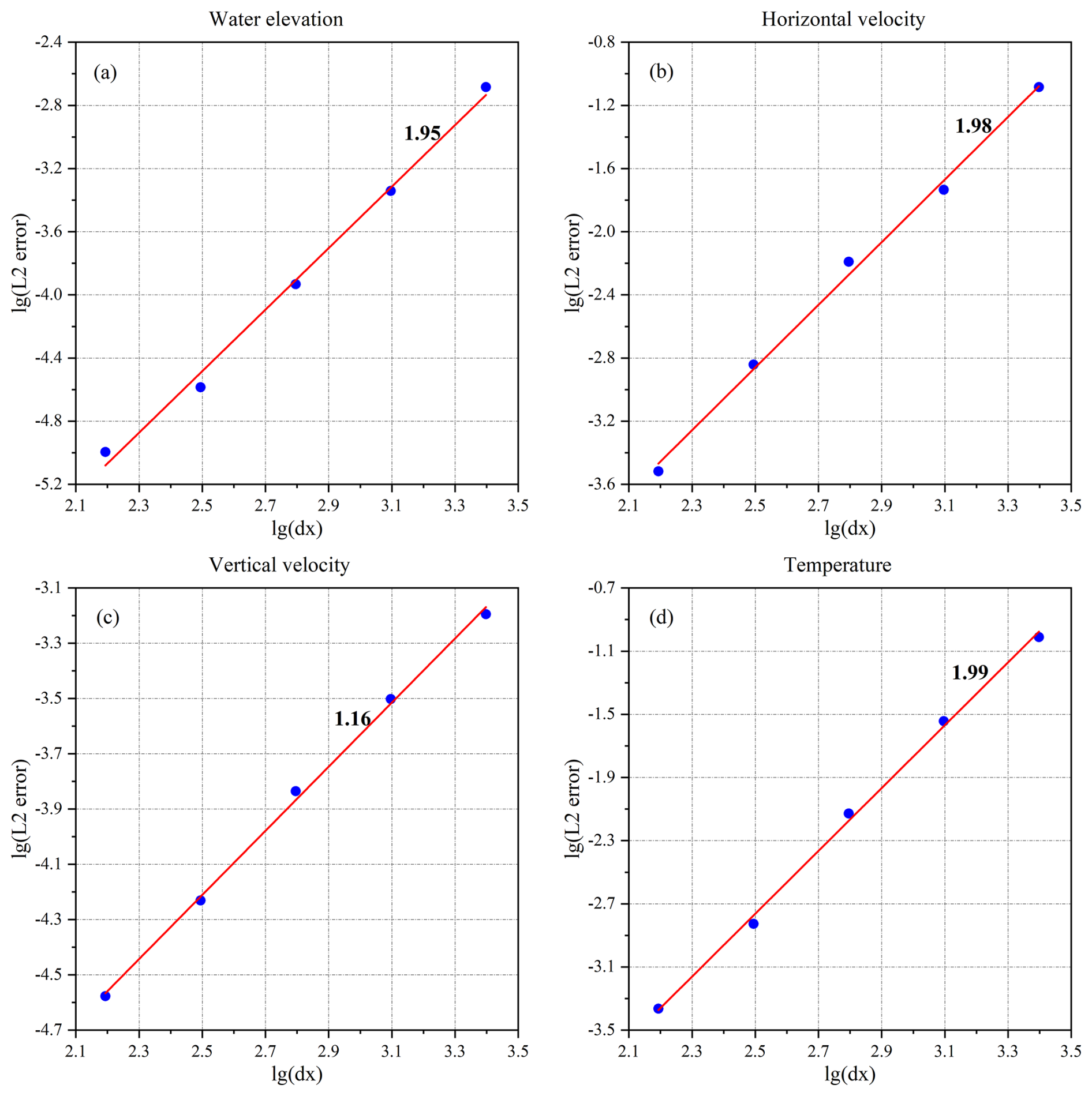
Figure 2 Convergence of the L₂ errors in the (a) surface elevation, (b) horizontal velocity, (c) vertical velocity, and (d) temperature field in the baroclinic manufactured solution test case.

For the five grid resolutions mentioned above, the model was run for 100 steps with time steps of 4.0, 2.0, 1.0, 0.5, and 0.25 s. The L₂ errors in the water elevation, horizontal velocity, vertical velocity, and temperature field across the entire computational domain were calculated, as shown in Fig. 2. The red lines shown in the figure represent the best-fit lines obtained using the least-squares method, with their slopes indicating the order of convergence. For varying grid resolutions, the water elevation, horizontal velocity, and temperature exhibit near-second-order convergence. However, the vertical velocity fails to achieve second-order convergence, which is attributed to the use of the vertically averaged continuity equation in the vertical velocity computation. The numerical solution of this equation inherently contains errors that accumulate throughout the calculation process, preventing the vertical velocity from reaching optimal second-order convergence. Overall, the results from this artificial analytical solution test are consistent with those of Kärnä et al. (2018), confirming that the discretisation of the advection term, baroclinic term, and Coriolis term in σ coordinates is accurate at both the coding and the algorithmic levels.

3.2 Lock exchange

In this subsection, we validate the baroclinic term and discuss the spurious mixing caused by horizontal diffusion with a standard lock exchange test (Ilıcak et al., 2012; Petersen et al., 2015; Kärnä et al., 2018). The computational domain is a rectangular channel that is 64 km long, 1 km wide, and 20 m deep. Each element in the domain is Δx = 500 m of the triangle edge length and 1 m in the vertical direction (total of 20 layers). The initial salinity is set to a constant value of 35 psu in the whole domain, and the initial temperature is calculated by

$$\begin{array}{}\text{(31)}& T(x,y,\mathit{\sigma })=\mathrm{5}\mathrm{°}\mathrm{C}\text{ where }\mathrm{0}\le x<\mathrm{32}\mathrm{km},\end{array}$$

$$\begin{array}{}\text{(32)}& T(x,y,\mathit{\sigma })=\mathrm{35}\mathrm{°}\mathrm{C}\text{ where }\mathrm{32}\le x\le \mathrm{64}\mathrm{km}.\end{array}$$

We use Eq. (7) to update the density, where α_T=0.2, β_S=0, T₀ = 5 °C, and S₀ = 35 psu. At the location of x = 32km, the initial density difference is ρ = 6.0 kg m⁻³. In the model, only the convective term controls the tracer concentration, and the bottom friction is omitted. The vertical viscosity, K_v, is 10⁻⁴ m² s⁻¹, and the horizontal viscosity, K_h, is varied with a value of 1, 10, and 200 m² s⁻¹ so that the grid Reynolds numbers $\mathit{Re}=U_{\text{grid}}\mathrm{\Delta }x/K_{\mathrm{h}}$ = 250.0, 25.0, and 1.25, where U_grid = 0.5 m s⁻¹ represents the characteristic velocity scale.

Figure 3 The density in the lock exchange test under three different grid Reynolds numbers.

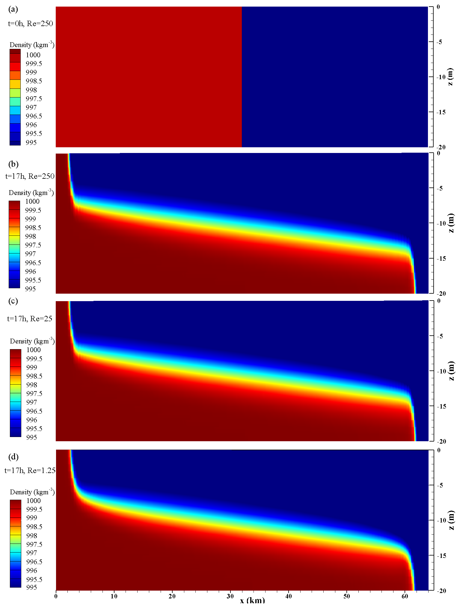
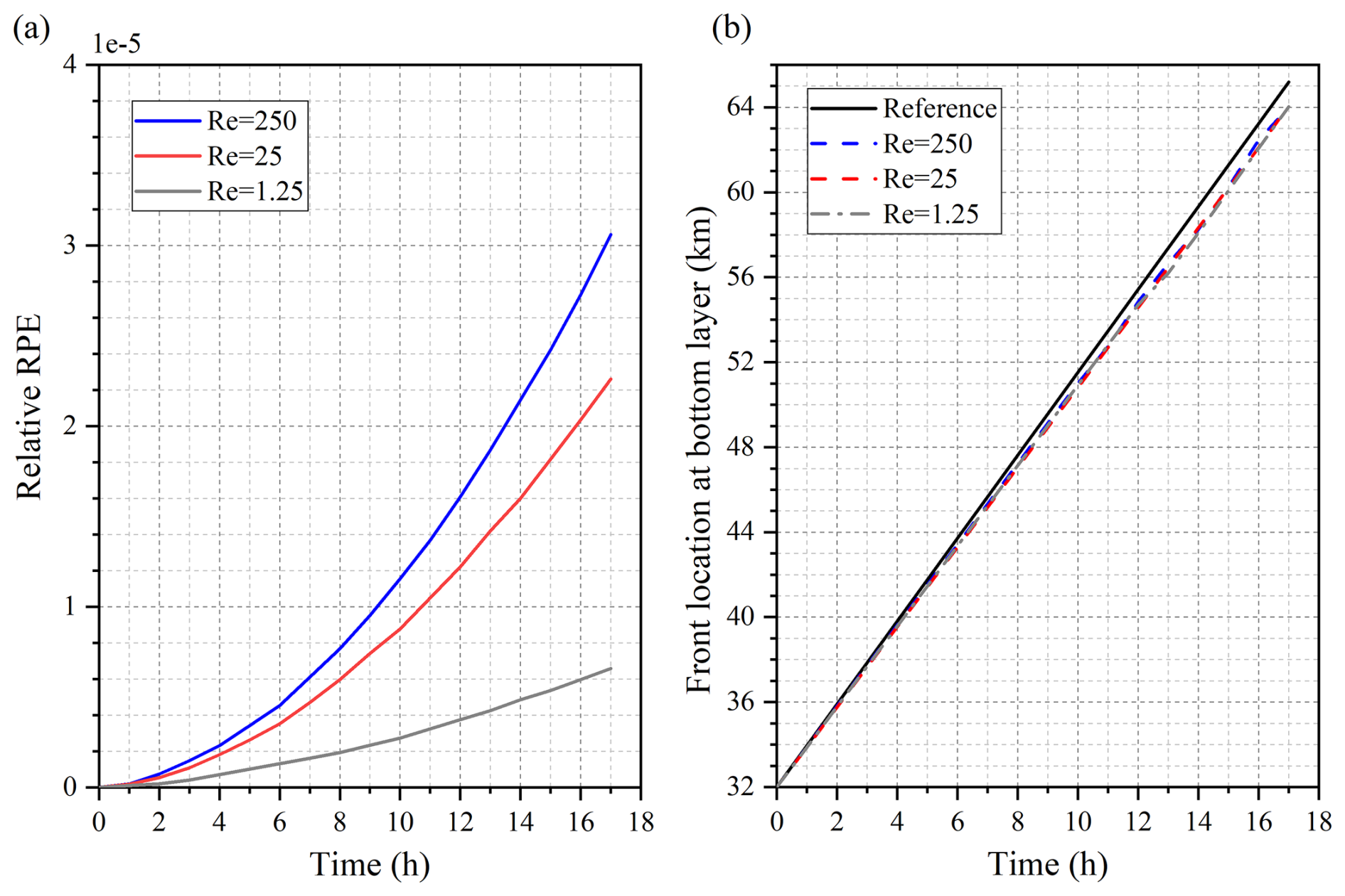
Figure 4 Simulation results of (a) relative RPE and (b) the density front location at the bottom layer of the lock exchange test with different Re.

Figure 3a shows the initial density field, and Fig. 3b–d are the density fields at the time of 17 h, where the Re values are 250.0, 25.0, and 1.25, respectively. It seems that as the Re decreases, the density front becomes smoother, indicating that the increase in background viscosity reduces overall mixing within the system. To quantify the role of spurious mixing, we also use a reference potential energy (RPE), which can be defined as

$$\begin{array}{}\text{(33)}& \text{RPE}=g\int {\mathit{\rho }}^{\ast }(z+D)\mathrm{d}z,\end{array}$$

where ρ^∗ is rearranged in descending order based on actual density values ρ from the bottom to the top. Using this computational approach, RPE represents the potential energy within the system that cannot be converted into kinetic energy. When spurious mixing is present, the value of RPE in the system increases. At any given time, t, the dimensionless relative reference potential energy ($\stackrel{\mathrm{‾}}{\text{RPE}}\left(t\right)$) is defined as follows:

$$\begin{array}{}\text{(34)}& \stackrel{\mathrm{‾}}{\text{RPE}}\left(t\right)={\displaystyle \frac{\text{RPE}\left(t\right)-\text{RPE}\left(\mathrm{0}\right)}{\text{RPE}\left(\mathrm{0}\right)}}.\end{array}$$

The calculation results of $\stackrel{\mathrm{‾}}{\text{RPE}}\left(t\right)$ for the three Reynolds numbers are shown in Fig. 4a. At the 17th hour, the values of $\stackrel{\mathrm{‾}}{\text{RPE}}\left(\mathrm{17}\right)$ are 3.06, 2.26, and 0.66 × 10⁻⁵, which agree with previous simulation results (Ilıcak et al., 2012; Kärnä et al., 2018). Additionally, the locations of the density fronts simulated under three different grid Reynolds number conditions were captured and compared with the theoretical maximum propagation distance, L, where $L=t/\mathrm{2}\sqrt{gD\mathrm{\Delta }\mathit{\rho }/{\mathit{\rho }}_{\mathrm{0}}}$. The spurious mixing resulted in a loss of potential energy throughout the system, leading to discrepancies between the model simulations and the theoretical values (Fig. 4b). Overall, the error remains within 4.7 %, which is consistent with Kärnä et al. (2018).

3.3 An ideal river plume

We continue to experiment with an ideal river plume (Wu 2023) to analyse the model's performance. Saltwater can be replaced by various contaminants that affect water quality. Therefore, investigating surface plume dynamics not only validates the model's accuracy but also highlights its applicability to environmental modelling and pollutant transport simulations.

Figure 5 The topography of the ideal river plume experiment.

3.3.1 Settings

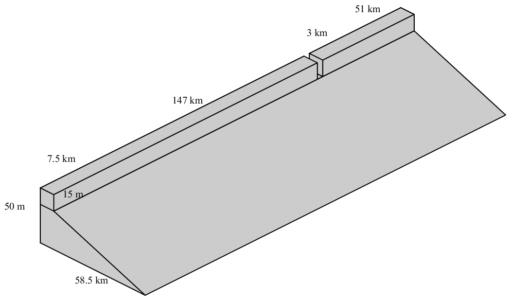
Figure 5 shows the topography of the estuary region, where there is a 7.5 km long, 3.0 km wide, and 15 m deep river that connects to the sea. The initial computational mesh domain is shown in Fig. 6. Freshwater runoff with a rate of 1500 m³ s⁻¹ and a salinity of 0 flows into a shelf with a bottom slope of 0.0007, where the salinity of the ocean water is 32 psu. We first use a grid resolution of 1500 m to partition the computational domain, which means that there are only two rows of grids along the width of the river channel. In this test, the Coriolis parameter is calculated by the latitude of 45° N, which is about 0.0001; the bottom friction coefficient is calculated by the MY-2.5 turbulent closure scheme with a bottom roughness parameter of 0.2 mm; and the eddy diffusivity coefficient is set to 0. Other external forces are not considered in this test. The open boundary is set to radiative according to Wu (2023) so that the boundary will have less influence on the currents in the computational domain. We also use Eq. (7) to update the density, where α_T=0, β_S=0.78, T₀ = 20 °C, and S₀ = 32 psu.

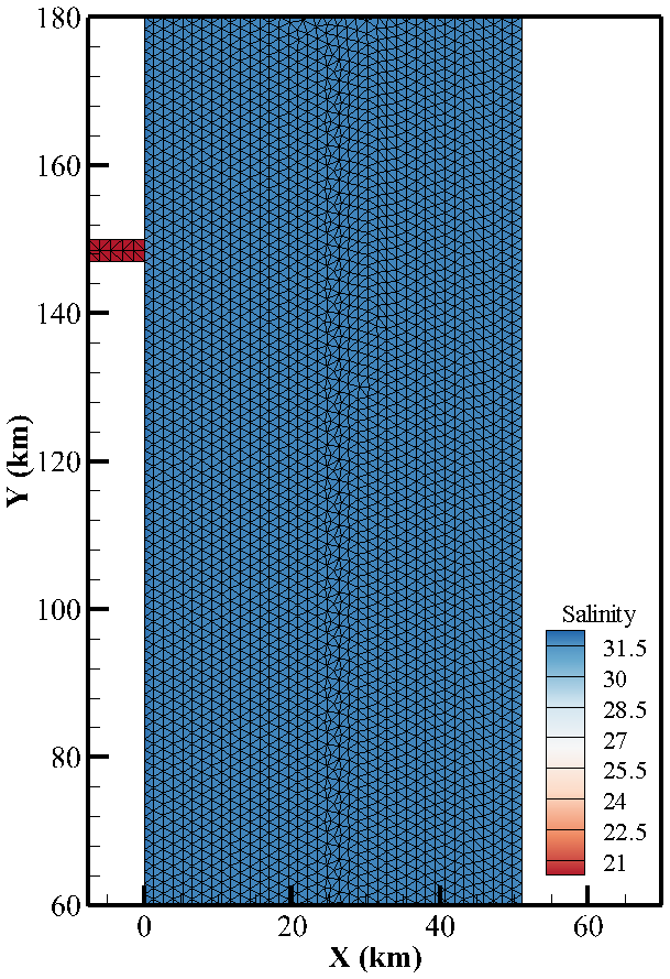
Figure 6 The computational mesh domain and the initial salinity field. The salinity is 0 psu at x < 0 km and 32 psu at x≥ 0 km.

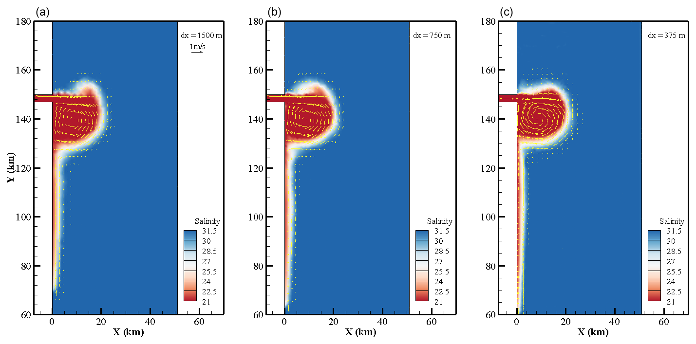
Figure 7 Simulated surface river plume and surface current velocity at 48 h. The grid resolution is refined from 1500 m (a) to 375 m (c).

3.3.2 Analysis of plume pattern

Due to the lack of analytical solutions in the test, we illustrate the accuracy of the simulation results from the perspective of grid convergence. For numerical methods, we prefer them to be less affected by grid resolution. Here, the mesh resolution is refined by a factor of 2 and 4 in both the x and the y directions, and the simulated results at 48 h are shown in Fig. 7. Considering the impact of differences in grid resolution on images, the simulation results of the three types of grids were processed in the same way to minimise the impact of post-processing as much as possible. Based on the simulated plume pattern, as the computational grid resolution increases, the zigzag phenomenon at the plume front gradually diminishes, resulting in a smoother edge and a more pronounced bulge shape. Simultaneously, there are noticeable differences in the extent of freshwater transport along the coast; with higher grid resolution, the transport distance increases. This may be attributed to the finer grid's ability to more accurately capture buoyancy fronts, thereby enhancing the coastal extension of freshwater. Additionally, the finer resolution reduces numerical dissipation, contributing to the observed differences in transport distance.

3.3.3 Quantitative analysis

To further demonstrate the performance of the model, a series of quantitative methods are employed to analyse the numerical simulation results of freshwater content (Fc in short), plume characteristics in the near- and mid-field regions, and coastal plume transport in the far-field region under different computational grid resolutions.

Following the concept of the isohaline coordinate by MacCready et al. (2002), the calculation method of freshwater volume can be written as

$$\begin{array}{}\text{(35)}& V\left(S^{\ast }\right)=\underset{S<S^{\ast }}{\int }(S_{\mathrm{0}}-S)/S_{\mathrm{0}}\mathrm{d}V,\end{array}$$

where S^∗ represents each salinity level. Then, we have

$$\begin{array}{}\text{(36)}& \text{Fc}\left(S\right)={\displaystyle \frac{\mathrm{d}V\left(S\right)}{\mathrm{d}S}}.\end{array}$$

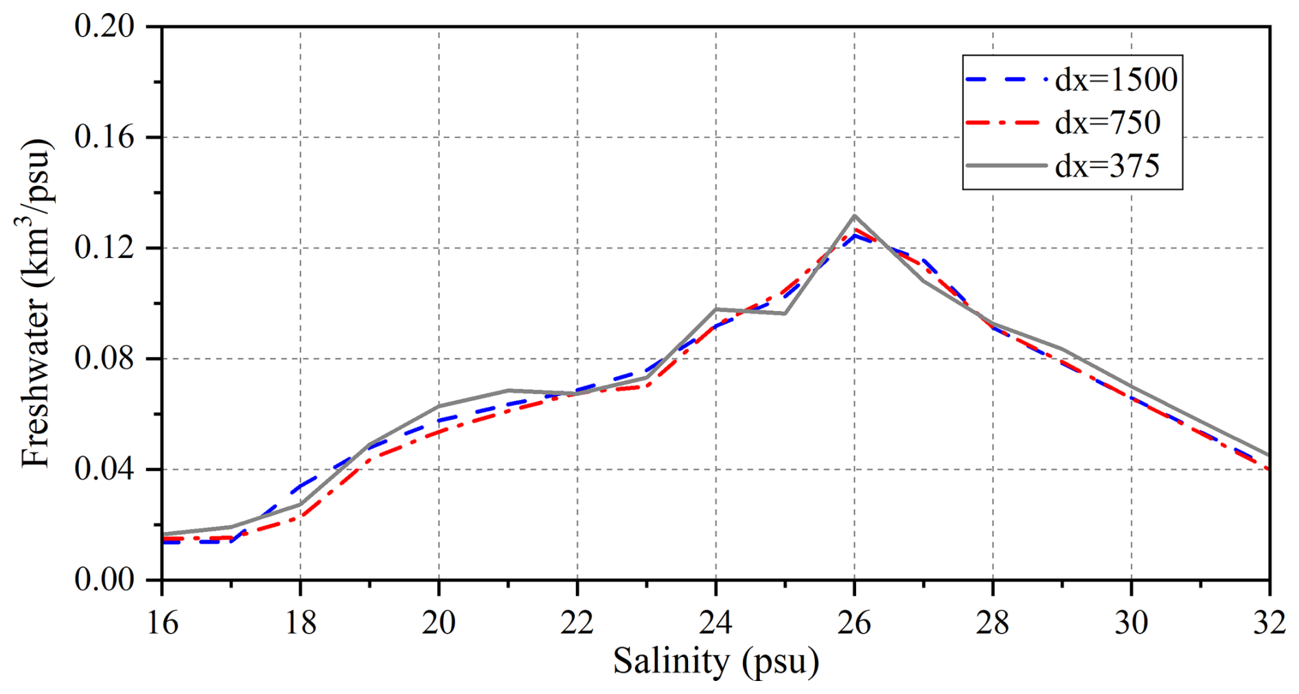
Figure 8 Freshwater content per salinity class at 48 h for results with different grid resolutions.

It can be seen in Fig. 8 that under the three grid resolutions, the freshwater content exhibits a similar trend: it increases initially and then decreases as salinity rises, with the peak freshwater content occurring at a salinity of 26 psu. This behaviour can be explained by the relationship between salinity and the distance from the river mouth. Lower salinity values indicate proximity to the river mouth, where the number of grids is relatively small, resulting in lower freshwater content in these regions. Conversely, higher salinity values correspond to regions farther from the river mouth, where more grids are present, but the freshwater content per cell is low, leading to lower overall freshwater content in high-salinity areas. These results are consistent with the research of Wu (2023).

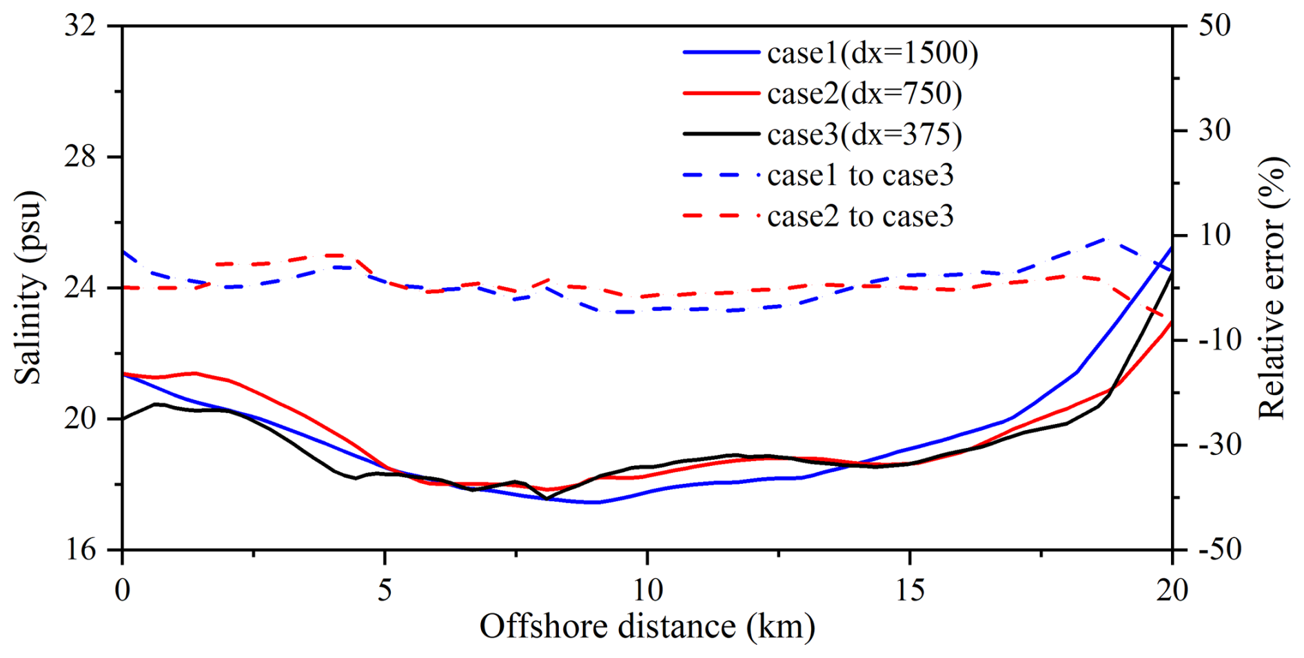
Figure 9 Surface salinity at the profile of y = 140 km under three grid resolutions. Dashed blue and red lines are the relative salinity errors for grid sizes of 1500 and 750 m, respectively, compared to the 375 m grid.

Secondly, at y = 140 km, approximately at the location of the plume's rotational centre, a cross-sectional profile was extracted to analyse the effect of grid resolution on the formation of the bulge in the near- and mid-field regions (see Fig. 9). When the grid resolution is 1500 m, the salinity at the centre of the bulge is relatively low, around 17.5 psu. As the grid resolution increases, the asymmetry of surface salinity from the centre of the bulge toward the edge of the inertial radius becomes more pronounced. Using the 375 m grid resolution as the reference, when the grid resolution is doubled or quadrupled, the salinity error relative to the reference case fluctuates within 10 %.

Finally, at y = 100 km, the relative freshwater transport carried by the coastal buoyancy current induced by the plume is calculated to assess the impact of grid resolution on the simulation results in the far-field region. The relative freshwater transport is determined by the ratio of the freshwater content at this location to that at the river mouth. At y = 100 km, the simulated surface coastal current velocity is consistently 0.30 m s⁻¹ across all grid resolutions, indicating minimal influence of grid resolution on current velocity. The percentage of freshwater transport at this location is 59.4 %, 57.5 %, and 60.6 % for grid resolutions of 1500, 750, and 375 m, respectively.

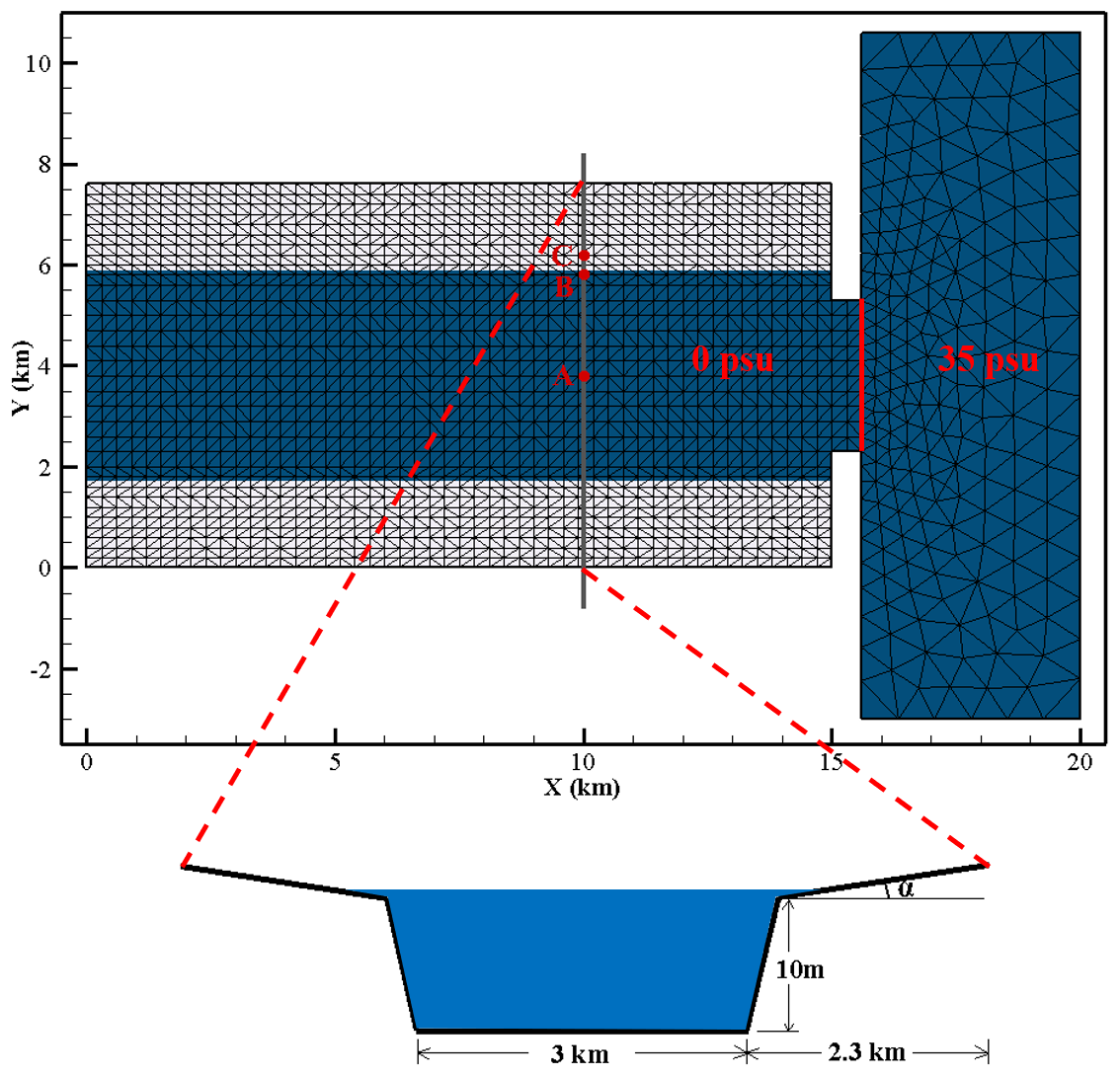
Figure 10 The calculation domain and its grid division of the semi-closed estuary. The minimum grid resolution is 200 m. The river channel cross-section is symmetric along the channel centreline and uniform along the channel direction. The initial water depth is 10.2 m and α = 0.0007. Three characteristic points are marked: the channel centre (A), the WD boundary (B), and the initially dry location (C). The initial salinity is set to 0 on the left side of the solid red line and 35 psu on the right side.

3.4 Saltwater enters an idealised semi-enclosed estuary

In addition to estuarine freshwater plumes, another phenomenon related to saltwater and freshwater interactions is saltwater intrusion into estuaries under tidal forcing. In this section, a semi-enclosed idealised river channel is configured, as shown in Fig. 10. This test case follows the setup described by Chen et al. (2022), with the computational mesh redefined accordingly. The channel is 15 km long, 3 km wide, and 10.2 m deep, with an initial salinity of 0. The channel features a riverbank slope of 0.033 and a floodplain slope of 0.0007. The right boundary is open to the sea, with a salinity of 35 psu, where a semi-diurnal tide with a 1 m amplitude is applied. The water temperature is uniformly set to 20 °C. Given that existing 3D DG baroclinic models lack empirical validation for handling WD processes, this test examines the model's applicability and reliability in solving the salinity transport equation in the presence of WD boundaries. The computational domain features a grid resolution ranging from 200 to 800 m, with the vertical dimension divided into 10 layers. The model operates with a time step of 0.2 s. The linear state equation is applied again, with α_T=0, β_S=0.714, T₀ = 20 °C, and S₀ = 35 psu, to update the density. The horizontal and vertical viscosities are set to 0.01 m² s⁻¹, the bottom friction coefficient is set to 0.005, and the threshold water depth is set to 0.05 m. The limiters mentioned in Sect. 2.3 are all applied to maintain robustness.

Figure 11 A 3D view of a flooding time.

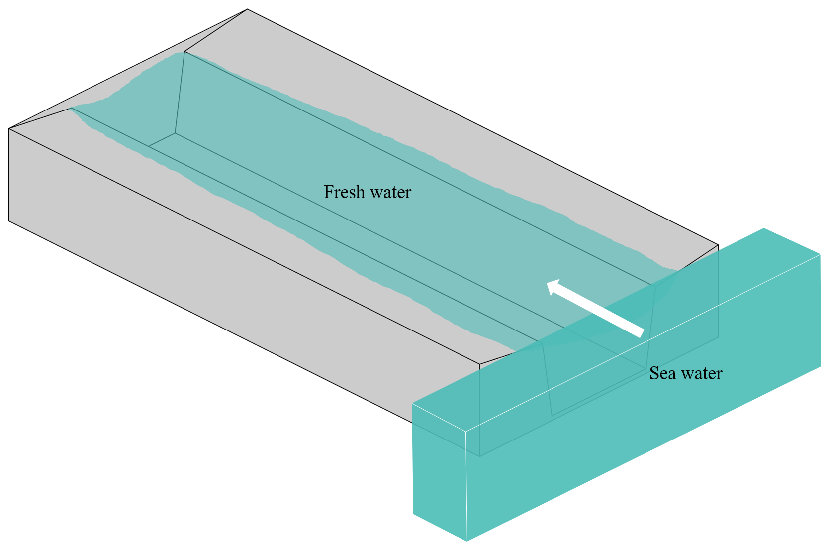
During the flood tide, seawater from the open boundary flows into the semi-closed channel and overtops the floodplain (Fig. 11). Three representative points were selected to analyse temporal variations in tidal water elevation and velocities: site A, located at the centre of the channel; site B, near the WD interface on the top of the riverbank slope at the initial time; and site C, situated in the initially dry intertidal zone (Fig. 10). At sites A and B, the surface water elevations exhibit nearly identical variations over a lunar day. However, at site C, water levels show periodic fluctuations only during the 8 h corresponding to the high-water time, remaining 0 the rest of the time (Fig. 12a). For site A, the mean velocity in the along-channel direction exhibits well-defined periodic variation, while the mean velocity in the cross-channel direction remains close to 0, indicating that the velocity field within the channel is minimally affected by the WD boundary treatment. For site B, the mean velocity in the along-channel direction is generally similar to that of site A. However, during the two flood tide phases, the velocity is slightly reduced due to the influence of the wetting and drying boundary treatment. In contrast, the mean velocity in the cross-channel direction shows periodic variation consistent with the tidal cycle. At site C, velocity is only observed during high water levels, with both the magnitude and the direction of the velocity varying during the 8 h window of tidal inundation (Fig. 12b and c). Moreover, the salinity variations along the channel centreline are shown in Fig. 13. As seawater intrudes from the estuarine mouth, the salinity values within the channel progressively increase in the negative x direction. Vertically, the salinity distribution exhibits a characteristic pattern of lower salinity near the surface and higher salinity near the bottom. Although this numerical experiment may not provide highly quantitative conclusions, the model's simulation results of the saltwater intrusion process involving WD interfaces are consistent with physical expectations.

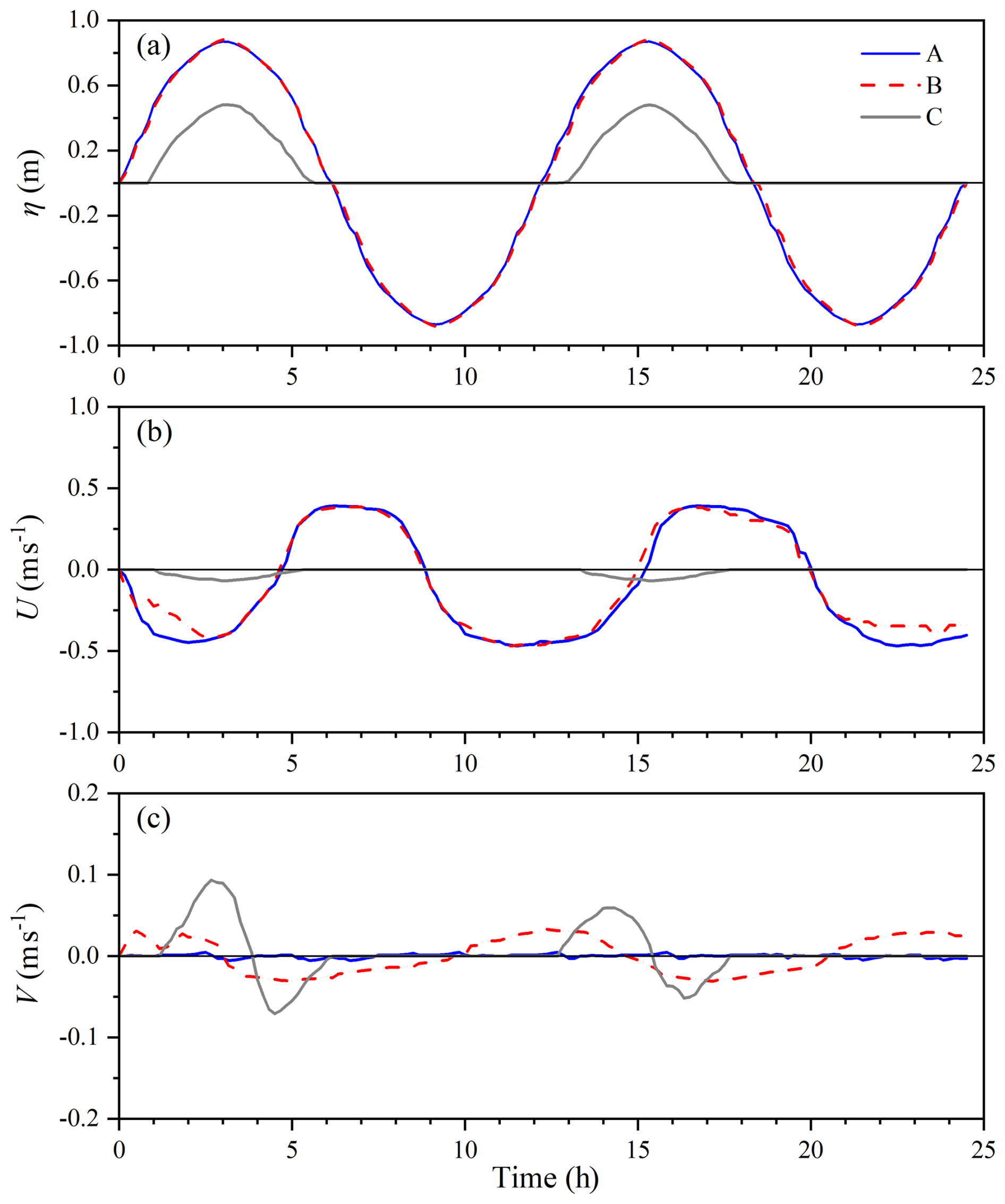
Figure 12 Time series of surface water elevation (a), depth-averaged velocity along the channel (b), and depth-averaged velocity across the channel (c) at points A, B, and C.

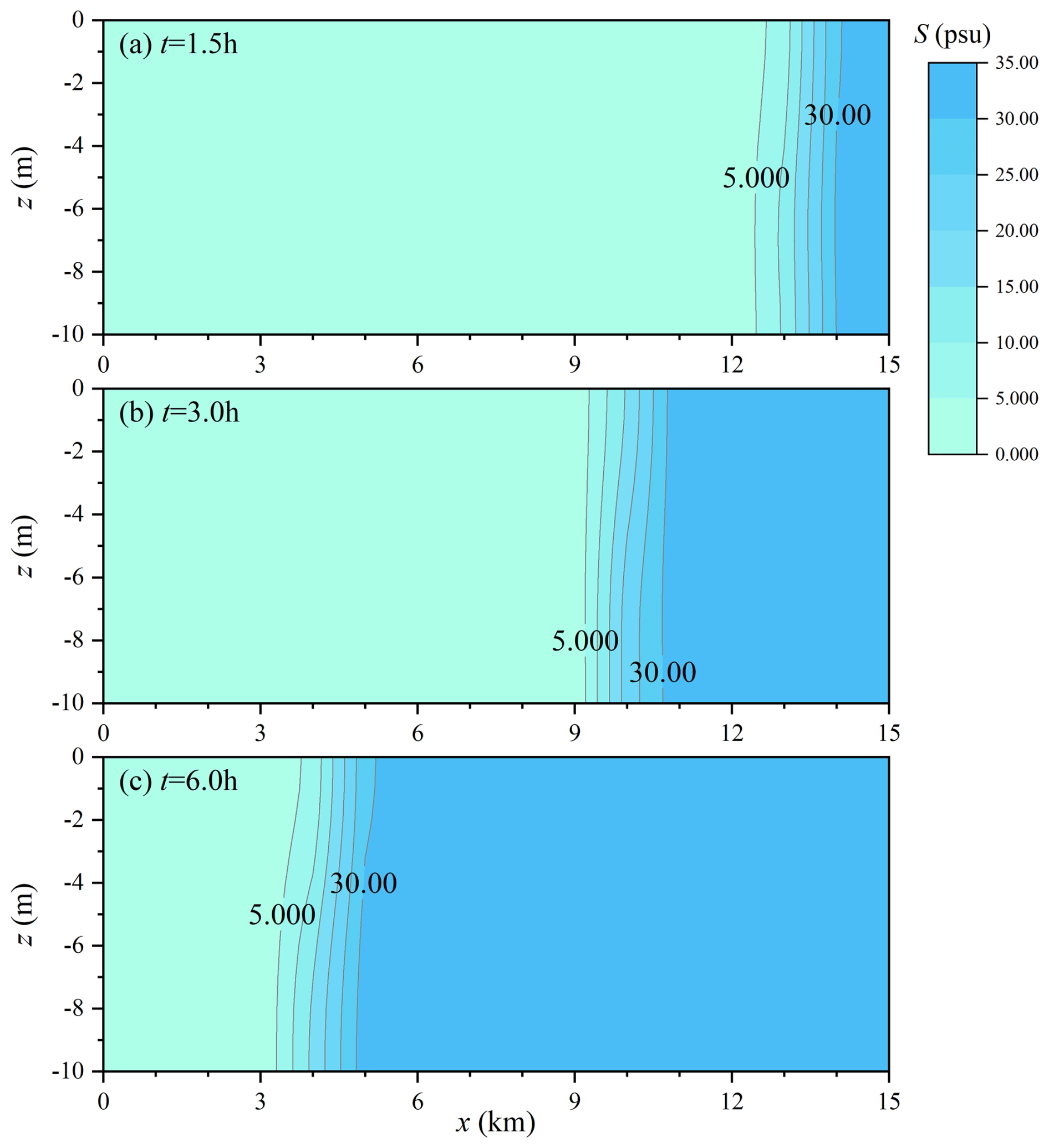
Figure 13 Salinity distribution along the channel centreline cross-section at 1.5, 3, and 6 h.

4 Conclusions

This study presents the development of a novel 3D discontinuous Galerkin coastal and estuarine modelling system, DGCEMS. The model distinguishes itself from existing 3D DG-based ocean models by employing σ coordinates, a nonsplit-mode framework, and a quadrature-free nodal discontinuous Galerkin method. A semi-implicit Runge–Kutta scheme is applied in the model. The code is available at https://doi.org/10.5281/zenodo.14803724 (Chen, 2025). Numerical tests show that the simulation results of the model have a second-order convergence for surface water elevation, horizontal velocity, and tracer fields, while the convergence of the vertical velocity field is approximately first order. The spurious mixing is also well controlled and comparable to the existing 3D DG coastal ocean model Thetis. The new model demonstrates low sensitivity to changes in grid resolution when simulating surface river plumes, consistently producing comparable results even with relatively coarse grids, and it has the capability to simulate salt–freshwater interactions in the presence of wetting and drying boundaries. In future work, the model will be further optimised in terms of its parallel computing strategy and overall solution framework to improve computational efficiency and scalability. Additional physical processes and modules, such as wave–current interactions, sediment transport, and biogeochemical dynamics, will also be incorporated to enhance the model's capability in simulating more complex and realistic estuarine and coastal systems.

Appendix A: Terms for the baroclinic manufactured solution test

Using Eqs. (28)–(30), the steady-state solution for other fields and terms are

$$\begin{array}{}\text{(A1)}& {\displaystyle }\mathit{\eta }=\mathrm{0},\text{(A2)}& {\displaystyle }U={\displaystyle \frac{\mathrm{1}}{\mathrm{6}}}\sin \left(\mathrm{3}\right)\sin \left(\mathrm{2}\mathit{\pi }x{L}_x\right),\text{(A3)}& {\displaystyle }V={\displaystyle \frac{-\mathrm{4}}{\mathrm{3}}}{\sin }^{\mathrm{2}}\left({\displaystyle \frac{\mathrm{1}}{\mathrm{4}}}\right)\cos \left({\displaystyle \frac{\mathit{\pi }y}{L_y}}\right),\text{(A4)}& {\displaystyle }\begin{array}{rl}\mathit{\omega }=& -{\displaystyle \frac{D\mathit{\pi }}{\mathrm{3}{L}_x{L}_y}}\left(L_y\cos \left({\displaystyle \frac{\mathrm{2}\mathit{\pi }x}{L_x}}\right)\left(\sin \right(\mathrm{3})+\sin (\mathrm{3}\mathit{\sigma }\left)\right)\right.\\ & \left.+\mathrm{2}{L}_x\left(-\cos \left({\displaystyle \frac{\mathrm{1}}{\mathrm{2}}}\right)+\cos \left({\displaystyle \frac{\mathit{\sigma }}{\mathrm{2}}}\right)\right)\sin \left({\displaystyle \frac{\mathit{\pi }y}{L_y}}\right)\right),\end{array}\text{(A5)}& {\displaystyle }\begin{array}{rl}{\displaystyle \frac{\partial DU}{\partial x}}& +{\displaystyle \frac{\partial DV}{\partial y}}={\displaystyle \frac{D\mathit{\pi }}{\mathrm{3}{L}_x{L}_y}}\left(L_y\sin \left(\mathrm{3}\right)\cos \left({\displaystyle \frac{\mathrm{2}\mathit{\pi }x}{L_x}}\right)\right.\\ & \left.+\mathrm{4}{\sin }^{\mathrm{2}}\left({\displaystyle \frac{\mathrm{1}}{\mathrm{4}}}\right)L_x\sin \left({\displaystyle \frac{\mathit{\pi }y}{L_y}}\right)\right),\end{array}\text{(A6)}& {\displaystyle \frac{\partial Duu}{\partial x}}={\displaystyle \frac{D\mathit{\pi }}{\mathrm{2}{L}_x}}{\cos }^{\mathrm{2}}\left(\mathrm{3}\mathit{\sigma }\right)\sin \left({\displaystyle \frac{\mathrm{4}\mathit{\pi }x}{L_x}}\right),\text{(A7)}& {\displaystyle }\begin{array}{rl}{\displaystyle \frac{\partial Duv}{\partial y}}=& -{\displaystyle \frac{D\mathit{\pi }}{\mathrm{6}{L}_y}}\cos \left(\mathrm{3}\mathit{\sigma }\right)\sin \left({\displaystyle \frac{\mathit{\sigma }}{\mathrm{2}}}\right)\sin \left({\displaystyle \frac{\mathrm{2}\mathit{\pi }x}{L_x}}\right)\\ & \times \sin \left({\displaystyle \frac{\mathit{\pi }y}{L_y}}\right),\end{array}\text{(A8)}& {\displaystyle }\begin{array}{rl}{\displaystyle \frac{\partial Duv}{\partial x}}=& {\displaystyle \frac{D\mathit{\pi }}{\mathrm{3}{L}_x}}\cos \left(\mathrm{3}\mathit{\sigma }\right)\sin \left({\displaystyle \frac{\mathit{\sigma }}{\mathrm{2}}}\right)\cos \left({\displaystyle \frac{\mathrm{2}\mathit{\pi }x}{L_x}}\right)\\ & \times \cos \left({\displaystyle \frac{\mathit{\pi }y}{L_y}}\right),\end{array}\text{(A9)}& {\displaystyle \frac{\partial Dvv}{\partial y}}=-{\displaystyle \frac{D\mathit{\pi }}{\mathrm{9}{L}_y}}{\sin }^{\mathrm{2}}\left({\displaystyle \frac{\mathit{\sigma }}{\mathrm{2}}}\right)\sin \left({\displaystyle \frac{\mathrm{2}\mathit{\pi }y}{L_y}}\right),\text{(A10)}& {\displaystyle }\begin{array}{rl}{\displaystyle \frac{\partial u\mathit{\omega }}{\partial \mathit{\sigma }}}=& {\displaystyle \frac{D\mathit{\pi }\sin \left(\mathrm{3}\mathit{\sigma }\right)\sin (\mathrm{2}\mathit{\pi }x/L_x)}{\mathrm{2}{L}_x{L}_y}}\\ & \times \left(L_y\cos \left({\displaystyle \frac{\mathrm{2}\mathit{\pi }x}{L_x}}\right)\left(\sin \right(\mathrm{3})+\sin (\mathrm{3}\mathit{\sigma }\left)\right)\right.\\ & \left.+\mathrm{2}{L}_x\left(-\cos \left({\displaystyle \frac{\mathrm{1}}{\mathrm{2}}}\right)+\cos \left({\displaystyle \frac{\mathit{\sigma }}{\mathrm{2}}}\right)\right)\sin \left({\displaystyle \frac{\mathit{\pi }y}{L_y}}\right)\right)\\ & -{\displaystyle \frac{D\mathit{\pi }\cos \left(\mathrm{3}\mathit{\sigma }\right)\sin (\mathrm{2}\mathit{\pi }x/L_x)}{\mathrm{6}{L}_x{L}_y}}\\ & \times \left(\mathrm{3}{L}_y\cos \left(\mathrm{3}\mathit{\sigma }\right)\cos \left({\displaystyle \frac{\mathrm{2}\mathit{\pi }x}{L_x}}\right)\right.\\ & \left.-L_x\sin \left({\displaystyle \frac{\mathit{\sigma }}{\mathrm{2}}}\right)\sin \left({\displaystyle \frac{\mathit{\pi }y}{L_y}}\right)\right),\end{array}\end{array}$$

$$\begin{array}{}\text{(A11)}& {\displaystyle }\begin{array}{rl}{\displaystyle \frac{\partial v\mathit{\omega }}{\partial \mathit{\sigma }}}=& -{\displaystyle \frac{D\mathit{\pi }\cos (\mathit{\sigma }/\mathrm{2})\cos (\mathit{\pi }y/L_y)}{\mathrm{18}{L}_x{L}_y}}\\ & \times \left(L_y\cos \left({\displaystyle \frac{\mathrm{2}\mathit{\pi }x}{L_x}}\right)\left(\sin \right(\mathrm{3})+\sin (\mathrm{3}\mathit{\sigma }\left)\right)\right.\\ & \left.+\mathrm{2}{L}_x\left(-\cos \left({\displaystyle \frac{\mathrm{1}}{\mathrm{2}}}\right)+\cos \left({\displaystyle \frac{\mathit{\sigma }}{\mathrm{2}}}\right)\right)\sin \left({\displaystyle \frac{\mathit{\pi }y}{L_y}}\right)\right)\\ & -{\displaystyle \frac{D\mathit{\pi }\cos (\mathit{\pi }y/L_y)\sin (\mathit{\sigma }/\mathrm{2})}{\mathrm{9}{L}_x{L}_y}}\\ & \times \left(\mathrm{3}{L}_y\cos \left(\mathrm{3}\mathit{\sigma }\right)\cos \left({\displaystyle \frac{\mathrm{2}\mathit{\pi }x}{L_x}}\right)\right.\\ & \left.-L_x\sin \left({\displaystyle \frac{\mathit{\sigma }}{\mathrm{2}}}\right)\sin \left({\displaystyle \frac{\mathit{\pi }y}{L_y}}\right)\right),\end{array}\text{(A12)}& {\displaystyle }\begin{array}{rl}{\displaystyle \frac{\partial DuT}{\partial x}}=& {\displaystyle \frac{\mathrm{15}D\mathit{\pi }\cos \left(\mathrm{3}\mathit{\sigma }\right)}{\mathrm{4}{L}_x}}\left(\mathrm{4}\cos \left({\displaystyle \frac{\mathrm{2}\mathit{\pi }x}{L_x}}\right)\right.\\ & +\cos \left(\mathit{\sigma }\right)\left(-\sin \left({\displaystyle \frac{\mathit{\pi }x}{L_x}}\right)+\mathrm{3}\sin \left({\displaystyle \frac{\mathrm{3}\mathit{\pi }x}{L_x}}\right)\right)\\ & \left.\times \sin \left({\displaystyle \frac{\mathit{\pi }y}{L_y}}\right)\right),\end{array}\text{(A13)}& {\displaystyle }\begin{array}{rl}{\displaystyle \frac{\partial DvT}{\partial y}}=& {\displaystyle \frac{\mathrm{5}D\mathit{\pi }\sin (\mathit{\sigma }/\mathrm{2})}{L_y}}\left(\cos \left(\mathit{\sigma }\right)\cos \left({\displaystyle \frac{\mathrm{2}\mathit{\pi }y}{L_y}}\right)\right.\\ & \left.\times \sin \left({\displaystyle \frac{\mathit{\pi }x}{L_x}}\right)-\sin \left({\displaystyle \frac{\mathit{\pi }y}{L_y}}\right)\right),\end{array}\text{(A14)}& {\displaystyle }\begin{array}{rl}{\displaystyle \frac{\partial \mathit{\omega }T}{\partial \mathit{\sigma }}}=& {\displaystyle \frac{\mathrm{5}D\mathit{\pi }\sin \left(\mathit{\sigma }\right)\sin (\mathit{\pi }x/L_x)\sin (\mathit{\pi }y/L_y)}{L_x{L}_y}}\\ & \times \left(L_y\cos \left({\displaystyle \frac{\mathrm{2}\mathit{\pi }x}{L_x}}\right)\left(\sin \right(\mathrm{3})+\sin (\mathrm{3}\mathit{\sigma }\left)\right)\right.\\ & \left.+\mathrm{2}{L}_x\left(-\cos \left({\displaystyle \frac{\mathrm{1}}{\mathrm{2}}}\right)+\cos \left({\displaystyle \frac{\mathit{\sigma }}{\mathrm{2}}}\right)\right)\sin \left({\displaystyle \frac{\mathit{\pi }y}{L_y}}\right)\right)\\ & -{\displaystyle \frac{\mathrm{5}D\mathit{\pi }}{L_x{L}_y}}\left(\mathrm{3}{L}_y\cos \left(\mathrm{3}\mathit{\sigma }\right)\cos \left({\displaystyle \frac{\mathrm{2}\mathit{\pi }x}{L_x}}\right)\right.\\ & \left.-L_x\sin \left({\displaystyle \frac{\mathit{\sigma }}{\mathrm{2}}}\right)\sin \left({\displaystyle \frac{\mathit{\pi }y}{L_y}}\right)\right)\left(\mathrm{1}+\cos \left(\mathit{\sigma }\right)\right.\\ & \left.\times \sin \left({\displaystyle \frac{\mathit{\pi }x}{L_x}}\right)\sin \left({\displaystyle \frac{\mathit{\pi }y}{L_y}}\right)\right),\end{array}\text{(A15)}& {\displaystyle }{S}_{\text{baro},x}=-{\displaystyle \frac{\mathrm{15}{\mathit{\alpha }}_{\mathrm{T}}{D}^{\mathrm{2}}g\mathit{\pi }}{L_x{\mathit{\rho }}_{\mathrm{0}}}}\cos \left({\displaystyle \frac{\mathit{\pi }x}{L_x}}\right)\sin \left(\mathit{\sigma }\right)\sin \left({\displaystyle \frac{\mathit{\pi }y}{L_y}}\right),\text{(A16)}& {\displaystyle }{S}_{\text{baro},y}=-{\displaystyle \frac{\mathrm{15}{\mathit{\alpha }}_{\mathrm{T}}{D}^{\mathrm{2}}g\mathit{\pi }}{L_y{\mathit{\rho }}_{\mathrm{0}}}}\cos \left({\displaystyle \frac{\mathit{\pi }y}{L_y}}\right)\sin \left(\mathit{\sigma }\right)\sin \left({\displaystyle \frac{\mathit{\pi }x}{L_x}}\right),\text{(A17)}& {\displaystyle }{S}_{\mathrm{f},x}=-{\displaystyle \frac{fD}{\mathrm{3}}}\cos \left({\displaystyle \frac{\mathrm{2}\mathit{\pi }y}{L_y}}\right)\sin \left({\displaystyle \frac{\mathit{\sigma }}{\mathrm{2}}}\right),\text{(A18)}& {\displaystyle }{S}_{\mathrm{f},y}={\displaystyle \frac{fD}{\mathrm{2}}}\sin \left({\displaystyle \frac{\mathrm{2}\mathit{\pi }x}{L_x}}\right)\cos \left(\mathrm{3}\mathit{\sigma }\right).\end{array}$$

The above terms are added to the right-hand side of Eq. (3) as source terms to balance the initial fields.