A hybrid-grid global model for the estimation of atmospheric weighted mean temperature considering time-varying vertical adjustment rate in GNSS precipitable water vapour retrieval

The atmospheric weighted mean temperature (T_m) is a key parameter in global navigation satellite system (GNSS) water vapour retrieval and can convert the zenith wet delay (ZWD) into precipitable water vapour (PWV). However, there are some shortcomings in the existing T_m models, such as the detailed time-varying vertical adjustment rate not being considered. In addition, the spatiotemporal characteristics of T_m need to be further refined. Therefore, we developed a new global high-precision and high-spatiotemporal-resolution T_m model considering time-varying vertical adjustment rate using the latest European Centre for Medium-Range Weather Forecasts Reanalysis 5 (ERA5) atmospheric reanalysis data. Firstly, a new global grid T_m vertical adjustment rate model (NGGTm-H) was developed using the sliding-window algorithm. Secondly, the daily variation characteristics of T_m and its relationships with geographical situations were investigated. Finally, a new global hybrid-grid T_m model (NGGTm) considering time-varying vertical adjustment rate was developed. To verify the effectiveness of the proposed model, the NGGTm model was compared with the Bevis and global pressure and temperature 3 (GPT3) models using the T_m data recorded at 378 radiosonde stations in 2017 and the surface gridded T_m data calculated from the ERA5 reanalysis data. The results show that taking the surface gridded T_m data of ERA5 as reference values, the average root-mean-square error (RMSE) value calculated by the NGGTm model was 2.84 K, which was lower with 0.50, 0.18 and 0.06 K than those of the Bevis, GPT3-5 and GPT3-1 models, respectively. Meanwhile, taking the T_m from the radiosonde stations as the reference values, the mean bias and RMSE of the NGGTm model were 0.10 and 3.30 K, respectively, which exhibit the best accuracy and stability among the Bevis, GPT3-5 and GPT3-1 models.

1 Introduction

Precipitable water vapour (PWV), a basic component of the water cycle of the Earth, is a key parameter in climate variation and material and energy exchange research performed at the global scale (Huang et al., 2023b; Ding et al., 2022). PWV directly affects the ground temperature and air humidity (Rocken et al., 1997). Furthermore, PWV is highly active in the Earth's atmosphere and plays a crucial role in the formation and evolution of weather. Its temporal and spatial variations are essential for the development of clouds and rainfall (Philipona et al., 2005; Jin and Luo, 2009). Understanding the exact spatiotemporal features of global PWV variations holds immense practical importance for monitoring and forecasting catastrophic weather events and conducting research on climate change. However, PWV is highly susceptible to the underlying terrain, seasonal variations and other climate changes, causing its spatial distribution to change unevenly and rapidly over time. Therefore, accurately monitoring PWV poses a significant challenge (Wang et al., 2007; Wang and Zhang, 2009). Currently, the methods for deriving PWV mainly include radiosonde, ground-based detection, microwave radiometer and satellite remote sensing inversion methods (Alexandrov et al., 2009; Gui et al., 2017; Zeng et al., 2019). Each technology has its own set of advantages and limitations. Radiosondes, for example, are highly accurate in measuring meteorological parameters but are limited by their low spatiotemporal resolution, high observation costs and inability to provide real-time or near-real-time updates on PWV changes (Zhai and Eskridge, 1996). Microwave radiometers that operate in the microwave region of the electromagnetic spectrum, and satellite remote sensing that relies on infrared band detection, offer high detection accuracies. However, their effectiveness is limited by interference from weather conditions such as cloud, fog, rain and snow. In addition, these instruments are unable to provide profile information of PWV in the vertical direction, and this shortcoming restricts their applicability in PWV detection tasks (Dalu, 1986; Gao and Kaufman, 2003).

The global navigation satellite system (GNSS) has become a crucial technology for real-time and high-precision PWV detection with advantages of all-weather capability, a high temporal resolution, low costs and weather resistance (Zhao et al., 2018; Jiang et al., 2017; Manandhar et al., 2017; Huang et al., 2022). The precision of GNSS-derived PWV can be as high as 1 to 1.5 mm, with a temporal resolution of 0.5 h (Rocken et al., 1993; Adams et al., 2011). PWV can be inverted by multiplying the wet component of the zenith total delay (ZTD) with the water vapour conversion factor. The ZTD consists of two parts: the zenith hydrostatic delay (ZHD) and the zenith wet delay (ZWD). The ZTD is an important factor affecting high precision GNSS positioning and also the basic data for GNSS atmospheric research (Huang et al., 2023a; Zhu et al., 2022). According to the high-precision observation data provided by the GNSS base station network, high-precision ZTD information can be obtained through data processing with high-precision GNSS data processing software. The ZHD values, with strong variation regularity, can be calculated by a simple model using surface pressure data to obtain an accuracy at the millimetre level. However, the variation in ZWD influenced mainly by water vapour is difficult to investigate (Vedel et al., 2001). The ZWD can be computed by subtracting the ZHD from the ZTD. Among the parameters involved in PWV inversion, the atmospheric weighted mean temperature (T_m) is the key parameter for calculating the water vapour conversion factor. The accuracy of GNSS tropospheric water vapour retrievals can be significantly improved by using high-precision T_m data.

High precision T_m data can typically be calculated by integrating radiosonde data, atmospheric reanalysis data and numerical weather prediction data. However, the distribution of radiosonde stations is uneven, and there is a time delay in releasing atmospheric reanalysis data. In addition, numerical weather prediction data are subject to certain limitations, including low temporal resolution and slow update speed, which renders them unsuitable for real-time or near-real-time PWV monitoring (Zhang et al., 2017). To improve the calculation efficiency of T_m, it is necessary to build a real-time and high-precision T_m model to meet the needs of GNSS PWV inversion. Existing T_m models can be divided into two categories: meteorological parameter models and non-meteorological parameter models. By analysing the correlation between the surface temperature (T_s) and T_m and utilising 2 yr profile information from 13 radiosonde stations in North America, the Bevis formula was developed through linear regression analysis (Bevis et al., 1992). This formula can successfully retrieve PWV information in the zenith direction of the station using GPS observation data and introduced the concept of GPS in meteorological research for the first time. The linear regression model remains a reliable and convenient tool that is still widely used today. However, it is important to note that the coefficients of this model exhibit distinct characteristics based on the region and season in which it is applied. Therefore, recalculating the parameters of the model is necessary when applying the model in other regions (Ross and Rosenfeld, 1997; Emardson et al., 1998). With the continuous development of GNSS PWV detection technology, many researchers have refined and expanded the Bevis model regionally and developed other T_m models based on measured meteorological parameters. In addition to T_s, T_m is also related to P_s and e_s. The global single-factor T_m model and multifactor T_m model were developed, which showed better accuracy and reliability (Yao et al., 2014b). To achieve better results in the global range, Yao et al. (2014a) proposed a T_m linear regression model in each latitude interval region using the European Centre for Medium-Range Weather Forecasts (ECMWF) reanalysis data. In addition, neural network algorithms can be used to establish T_m models that can produce corresponding T_m values by simply using T_s information as the input. The accuracy of this model depends on the precision of the input T_s information. When highly precise T_s data were used, the model accuracy was increased (Ding, 2018). The above models have achieved good results when providing the required measured meteorological parameters, but most of the GNSS stations in the world do not have supporting meteorological sensors installed, leading to great difficulty in measuring meteorological parameters in real-time. Therefore, these models are difficult to apply to real-time or near-real-time GNSS PWV detection tasks. To address this issue, many researchers have developed T_m models (empirical models) that run without measured meteorological parameters. For example, Zhu et al. (2021) developed a new T_m model taking climate differences into account in the Shanxi region. The non-meteorological parameter T_m model (named the Emardson model) was developed to take the annual cycle variation into account by using radiosonde data collected in Europe over many years, which was capable of meeting the requirement for GNSS PWV detection (Emardson and Derks, 2000). Therefore, the model has been widely used in real-time GNSS meteorology research. In addition, the vertical adjustment rate is the key parameter in the T_m vertical adjustment. Taking the vertical adjustment rate into account can not only improve the T_m model accuracy, but also shows significant improvement in regions with undulating terrain (Huang et al., 2023c; Sun et al., 2021; Yao et al., 2018). The T_m vertical adjustment rate is an effective means of adjusting T_m to consider the varying topography height. Therefore, investigating the spatiotemporal variation characteristics of the T_m vertical adjustment rate and developing a T_m vertical adjustment rate model have high application values in T_m vertical and spatial interpolation tasks. Although the aforementioned models excel in certain regions and possess unique strengths, they are not suitable for calculating T_m at the global level. Yao et al. (2012) developed the first new global atmospheric weighted average temperature model (GWMT) using data from 135 radiosonde stations worldwide over several years. This new model can estimate the T_m value at any location by simply inputting the station location and the day of the year (DOY); the method has been applied to real-time GNSS PWV inversion studies worldwide. However, because the radiosonde data used in the GWMT model are all located on land, there is a certain systematic bias in ocean areas. To address this issue, the GTm-II model, GTm-III model and GTm-H model were developed (Yao et al., 2013). GPT series models which include GPT, GPT2, GPT2w and GPT3 also show excellent performance worldwide (Landskron and Böhm, 2018; Böhm et al., 2007, 2015; Yang et al., 2020). Although the latest GPT3 model is currently the most representative empirical model with a high precision on the global scale, GPT3 model does not take into account vertical adjustment or detailed T_m vertical adjustment rate. Thus, it is necessary to develop a new model to improve the real-time high-precision global empirical T_m model and to select appropriate data sources for model development.

The global T_m models mentioned above were established without accounting for the detailed time-varying vertical adjustment rate. Therefore, in this study, our aim was to develop a global T_m model that takes into account time-varying vertical adjustment rate and high-precision capabilities. To attain this objective we first investigated the spatiotemporal variations and characteristics of the vertical adjustment rate of global T_m and developed a new global grid vertical adjustment rate model (NGGTm-H). Second, a new global hybrid-grid model (NGGTm) for the estimation of atmospheric weighted mean temperature considering time-varying vertical adjustment rate was developed by using profile gridded T_m data calculated by integrating the latest European Centre for Medium-Range Weather Forecasts ReAnalysis 5 (ERA5) reanalysis data. To verify the effectiveness of the new model, the NGGTm model was compared with the Bevis and GPT3 models using T_m data from radiosonde stations and ERA5 reanalysis data.

The rest of our paper is organised as follows. In Sect. 2, we introduce the data, the method of obtaining T_m and the inversion method of PWV. In Sect. 3, we analyse the spatiotemporal characteristics of the T_m vertical adjustment rate and develop a T_m vertical adjustment rate model. In Sect. 4, we analyse the T_m temporal characteristics and develop a global T_m model (NGGTm). In Sect. 5, we describe the experiments on the validation of NGGTm. Finally, in Sect. 6, we provide the conclusions and suggestions for future work.

2 Data and methodology

2.1 Data

The ERA5 atmospheric reanalysis data, provided by ECMWF (https://cds.climate.copernicus.eu/datasets, last access: 23 September 2025), is the fifth-generation global climate reanalysis dataset. This dataset provides hourly surface-level parameters and pressure-level data with a horizontal resolution of 0.25°×0.25° (latitude×longitude) and a vertical resolution of 37 levels. ERA5 data can provide high-resolution and relatively complete surface-level and pressure-level data and are thus expected to be widely used in the future. The radiosonde station data can be downloaded for free from the University of Wyoming (http://weather.uwyo.edu/upperair/sounding.shtml, last access: 23 September 2025). This product provides meteorological layered data and surficial parameters such as PWV from the ground to the near-Earth space (an altitude of approximately 30 km) and provides radiosonde data twice a day (00:00 and 12:00 UTC); these data are often used as reference values for model verification tasks. The ERA5 gridded data from 2012 to 2017 and the radiosonde data in 2017 on the global scale were used to analyse and develop the model in this study.

2.2 Methodology

T_m is the key parameter used to convert ZWD into PWV. Using atmospheric reanalysis data, radiosonde data and other data, highly accurate T_m information can be obtained by integral calculation. In addition, the modelling method can also obtain T_m values at a high accuracy and with a high calculation efficiency. The specific T_m integral calculation formula is expressed as follows:

$$\begin{array}{}\text{(1)}& T_{\mathrm{m}}={\displaystyle \frac{{\int }_{h_{\text{bot}}}^{h_{\text{top}}}\frac{e}{T}\mathrm{d}H}{{\int }_{h_{\text{bot}}}^{h_{\text{top}}}\frac{e}{T^{\mathrm{2}}}\mathrm{d}H}},\end{array}$$

where h_bot and h_top are, respectively, the heights at the bottom and top of the integration calculation, T_m is the atmospheric weighted mean temperature at h_bot, e is the water vapour pressure (hPa), T is the temperature (K) and H is the height (m). The height corresponding to T_m is denoted by h_bot. Different values of h_bot correspond to different values of T_m. Therefore, the layered T_m can be calculated using Eq. (1).

The modelling methods used to calculate T_m can be divided into two categories: (1) T_m models based on measured meteorological parameters, of which the most representative is the Bevis model ($T_{\mathrm{m}}=\mathrm{70.2}+\mathrm{0.72}{T}_{\mathrm{s}}$), namely, the T_m linear regression model, and (2) non-meteorological parameter T_m models, of which the most classical is the GPT series model. The GPT3 model, the latest model in the GPT series, has a high accuracy in calculating global T_m. The GPT3 model formula used to calculate T_m can be expressed as follows:

$$\begin{array}{}\text{(2)}& \begin{array}{rl}{T}_{\mathrm{m}}^{\text{GPT3}}=& a_{\mathrm{0}}+a_{\mathrm{1}}\cos \left(\mathrm{2}\mathit{\pi }{\displaystyle \frac{\text{DOY}}{\mathrm{365.25}}}\right)+b_{\mathrm{1}}\sin \left(\mathrm{2}\mathit{\pi }{\displaystyle \frac{\text{DOY}}{\mathrm{365.25}}}\right)\\ & +a_{\mathrm{2}}\cos \left(\mathrm{4}\mathit{\pi }{\displaystyle \frac{\text{DOY}}{\mathrm{365.25}}}\right)+b_{\mathrm{2}}\sin \left(\mathrm{4}\mathit{\pi }{\displaystyle \frac{\text{DOY}}{\mathrm{365.25}}}\right)\end{array},\end{array}$$

where $T_{\mathrm{m}}^{\text{GPT3}}$ denotes T_m calculated by the GPT3 model, a₀ denotes the average annual value of T_m, a₁ and b₁ denote the annual cycle coefficient of T_m, a₂ and b₂ denote the semiannual cycle coefficient of T_m and DOY denotes the day of the year.

PWV refers to the total water vapour content of a vertical column per unit area in the atmosphere and can be converted from ZWD using the following formula:

$$\begin{array}{}\text{(3)}& \text{PWV}=\mathrm{\Pi }\times \text{ZWD},\end{array}$$

where Π denotes the PWV conversion factor. This conversion factor can be expressed as follows:

$$\begin{array}{}\text{(4)}& \mathrm{\Pi }={\displaystyle \frac{{\mathrm{10}}^{\mathrm{6}}}{{\mathit{\rho }}_w{R}_{\mathrm{v}}(k_{\mathrm{2}}^{\prime }+k_{\mathrm{3}}/T_{\mathrm{m}})}},\end{array}$$

where R_v denotes the water vapour gas constant, $k_{\mathrm{2}}^{\prime }$ and k₃ are constants ($k_{\mathrm{2}}^{\prime }=\mathrm{22.97}$ K hPa⁻¹ and k₃=375 463 K² hPa⁻¹) and the other parameters are described above. Therefore, T_m is the key parameter in the GNSS PWV inversion.

To facilitate the subsequent test of the accuracy of the T_m values calculated using the atmospheric reanalysis data and the performance of the new T_m model, this study uses the bias and root-mean-square error (RMSE) as the accuracy evaluation indicators. The formulas are expressed as follows:

$$\begin{array}{}\text{(5)}& {\displaystyle }\text{bias}={\displaystyle \frac{\mathrm{1}}{N}}{\sum }_{i=\mathrm{1}}^N({\text{Tm}}_{\mathrm{M}}^i-{\text{Tm}}_{\mathrm{R}}^i),\text{(6)}& {\displaystyle }\text{RMSE}=\sqrt{{\displaystyle \frac{\mathrm{1}}{N}}{\sum }_{i=\mathrm{1}}^N({\text{Tm}}_{\mathrm{M}}^i-{\text{Tm}}_{\mathrm{R}}^i{)}^{\mathrm{2}}},\end{array}$$

where N denotes the number of samples, ${\text{Tm}}_{\mathrm{M}}^i$ denotes the calculated value of the atmospheric reanalysis data or model and ${\text{Tm}}_{\mathrm{R}}^i$ denotes the reference value.

3 Development of the T_m vertical adjustment rate model

3.1 Analysis of the spatiotemporal characteristics of the T_m vertical adjustment rate

Given the discernible variations in topography and the significant range of height at a global scale, there can be considerable disparities between the height of atmospheric reanalysis data grid points and the actual heights of the ground-based GNSS receiver (named target height), so it is necessary to adjust T_m vertically. The previous study has analysed this topic and concluded that there is an approximately linear relationship between the layered T_m data and h_bot (Huang et al., 2019). To further analyse the variation in T_m with height, six representative ERA5 reanalysis data grid points ((60° N, 90° W), (60° N, 90° E), (0°, 90° W), (0°, 90° E), (60° S, 90° W) and (60° S, 90° E)) were selected globally to analyse the layered T_m data and corresponding height data on 1 January 2017. The results are shown in Fig. 1.

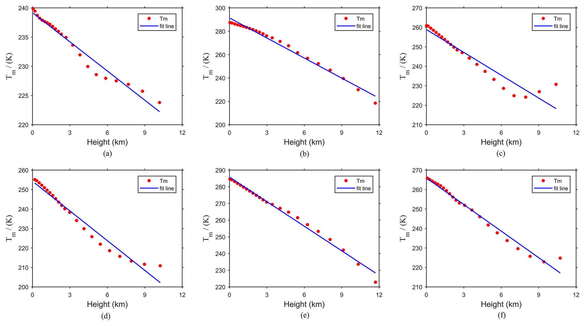
Figure 1 T_m changes with height at six representative ERA5 reanalysis data gridded points on 1 January 2017. (a) (60° N, 90° W). (b) (0°, 90° W). (c) (60° S, 90° E). (d) (60° N, 90° E). (e) (0°, 90° E). (f) (60° S, 90° W).

Figure 1 shows that the layered T_m data of six representative ERA5 reanalysis data grid cells exhibit approximate linear change relationships with height. Moreover, the layered T_m data gradually decrease with increasing height. Therefore, the slope of the fitting line represents the vertical adjustment rate of T_m, and this relation can be expressed as

$$\begin{array}{}\text{(7)}& T_{\mathrm{m}}=\mathit{\gamma }\times \mathit{\delta }h+l,\end{array}$$

where γ denotes the vertical adjustment rate of T_m, δh denotes the height difference and l denotes a constant.

To investigate the variation relationship between the vertical adjustment rate of T_m and time at the global scale, six representative ERA5 reanalysis data grid points were selected to calculate the vertical adjustment rate of T_m from 2012 to 2016. Furthermore, the time series for the vertical adjustment rate of the daily mean T_m from 2012 to 2016 was obtained and used to achieve seasonal fitting by the cosine function of the annual and semiannual periods. The results are shown in Fig. 2.

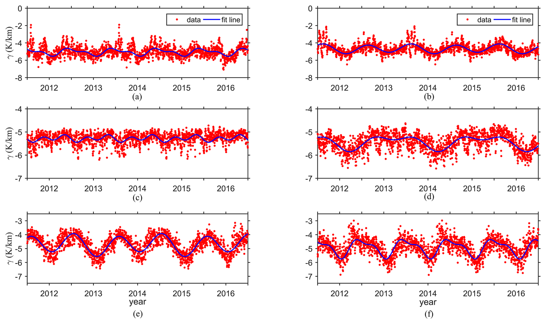
Figure 2 The time-series variations in the T_m vertical adjustment rate from the ERA5 reanalysis data at six representative grid points. (a) (60° N, 90° W). (b) (60° N, 90° E). (c) (0°, 90° W). (d) (0°, 90° E). (e) (60° S, 90° W). (f) (60° S, 90° E).

Figure 2 shows the obvious seasonal variations in the vertical adjustment rate of T_m calculated using the ERA5 reanalysis data at six representative grid points. From Fig. 2c and d, the annual and semiannual variations in the vertical adjustment rate of T_m are relatively slight at the grid points located on the Equator. However, From Fig. 2e and f, the vertical adjustment rate of T_m at the grid points located in the high-latitude areas of the Southern Hemisphere exhibit relatively large variation ranges and show obvious annual and semiannual variations, whereas those in the high-latitude areas of the Northern Hemisphere show slight variation ranges and obvious annual and semiannual cycle variations from Fig. 2a and b. The main reason for these results is that most of the high-latitude areas of the Southern Hemisphere are oceans and are thus not affected by complex climates.

Hence, a clear seasonal pattern is evident in the vertical adjustment rate of T_m, and the variation patterns vary across different regions. The vertical adjustment rate of T_m was then calculated with a temporal resolution of 1 h from 2012 to 2016 at the global scale. The annual mean value, annual cycle amplitude, semiannual cycle amplitude and daily cycle amplitude of the vertical adjustment rate of T_m were calculated by using Eq. (8) at selected grid points at the global scale. The utilised formula is expressed as follows:

$$\begin{array}{}\text{(8)}& \begin{array}{rl}\mathit{\gamma }=& A_{\mathrm{0}}+A_{\mathrm{1}}\cos \left(\mathrm{2}\mathit{\pi }{\displaystyle \frac{\text{DOY}}{\mathrm{365.25}}}\right)+A_{\mathrm{2}}\sin \left(\mathrm{2}\mathit{\pi }{\displaystyle \frac{\text{DOY}}{\mathrm{365.25}}}\right)\\ & +A_{\mathrm{3}}\cos \left(\mathrm{4}\mathit{\pi }{\displaystyle \frac{\text{DOY}}{\mathrm{365.25}}}\right)+A_{\mathrm{4}}\sin \left(\mathrm{4}\mathit{\pi }{\displaystyle \frac{\text{DOY}}{\mathrm{365.25}}}\right)\\ & +A_{\mathrm{5}}\cos \left(\mathrm{2}\mathit{\pi }{\displaystyle \frac{\text{HOD}}{\mathrm{24}}}\right)+A_{\mathrm{6}}\sin \left(\mathrm{2}\mathit{\pi }{\displaystyle \frac{\text{HOD}}{\mathrm{24}}}\right),\end{array}\end{array}$$

where γ is the vertical adjustment rate of T_m; A₀ is the annual mean value of the vertical adjustment rate of T_m; (A₁, A₂) are the annual cycle coefficients for the vertical adjustment rate of T_m; (A₃, A₄) are the semiannual cycle coefficients for the vertical adjustment rate of T_m; (A₅, A₆) are the daily cycle coefficients for the vertical adjustment rate of T_m; DOY is the day of the year; and the hour of the day (HOD) is the UTC time. The above coefficients were calculated at each grid point based on a least-square adjustment by using all selected grid points in the world from 2012 to 2016. The results are shown in Fig. 3.

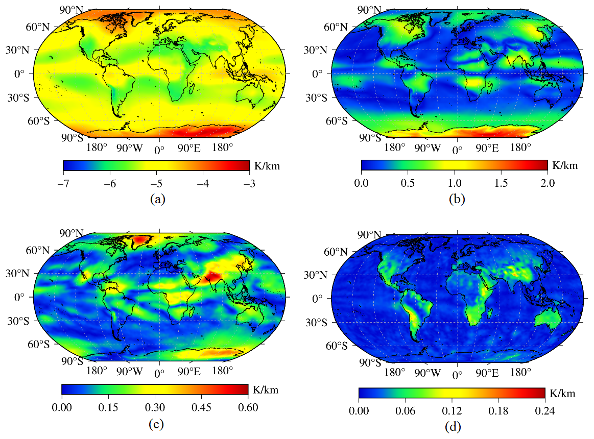
Figure 3 The distributions of the annual mean value and amplitudes of the T_m vertical adjustment rate calculated using global ERA5 reanalysis data. (a) Annual average value. (b) Annual cycle amplitude. (c) Semiannual cycle amplitude. (d) Daily cycle amplitude.

As shown in Fig. 3, a strong correlation was found between the annual mean T_m vertical adjustment rate and latitude. Regarding the annual cycle amplitude of the vertical adjustment rate of T_m, obvious annual cycle amplitude values were observed in most land areas, especially over the Antarctic continent, though these amplitudes were relatively small in the ocean and coastal areas located in the middle and low latitudes of the Northern and Southern Hemispheres. In addition, a sea–land difference was observed in the semiannual cycle amplitude of the T_m vertical adjustment rate. The daily cycle amplitude of the vertical adjustment rate of T_m remained at approximately 0.06 K km⁻¹. Since the daily variation in the vertical adjustment rate of T_m can be overshadowed by the annual and semiannual variations, we focused on optimising and simplifying the model coefficients when developing the T_m vertical adjustment rate model.

The above analysis demonstrated that the variation law of the vertical adjustment rate of T_m differs spatially. This makes it difficult to accurately grasp the variation law of the vertical adjustment rate of T_m in developing a global uniform model for the vertical adjustment rate of T_m. Therefore, we presents a solution to the issue of coefficient redundancy that can occur when developing a model from individual grid points. Specifically, a sliding-window algorithm was introduced to develop the T_m vertical adjustment rate model, leading to optimised coefficients and improved accuracy, stability and applicability of the model. Note that the sliding-window algorithm has been used in the previous study, which exhibits a superior performance (Huang et al., 2019).

3.2 Development of NGGTm-H

The ERA5 reanalysis data with a horizontal resolution of 0.25°×0.25° were selected as the data source to develop the model in this study. We divided global segments into regular windows with the same horizontal resolution as the ERA5 reanalysis data. The specific process was as follows: starting from the first window, by using the data of nine gridded points in each window, the model coefficients of the corresponding window were calculated in order from west to east and from north to south and stored at the geometric centre of the corresponding window. Finally, all the coefficients for the global T_m vertical adjustment rate model were obtained. As shown in Fig. 4, blue dots denote ERA5 gridded points, and red dots denote centre points of the window; the red rectangle denotes the size of the sliding window.

Figure 4 The realisation process of the sliding-window algorithm.

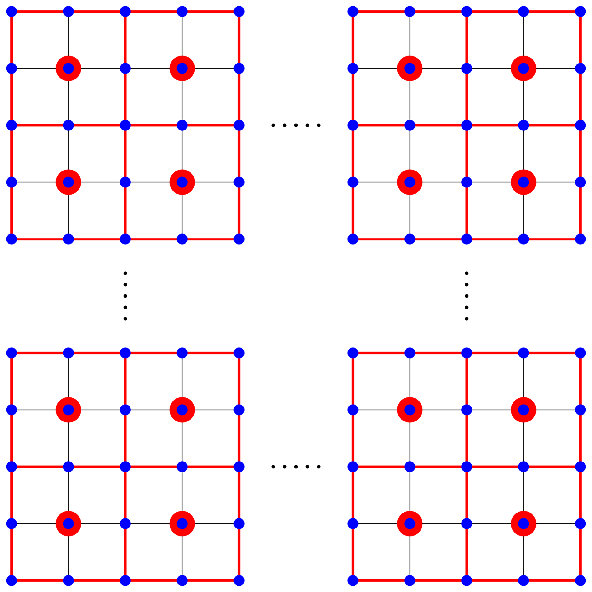
To investigate the influence of the window size on the model precision and optimise the model coefficients as much as possible, three different window sizes, with resolutions of 0.5°×0.5°, 1°×1° and 2°×2°, were selected to develop the model. The window with the resolutions of 0.5°×0.5°, 1°×1° and 2°×2° contains 9, 25 and 49 gridded points, respectively. As mentioned above, it was necessary to consider the characteristics of the annual and semiannual cycles when developing the model. Therefore, the formula of the global T_m vertical adjustment rate model in each window can be expressed as follows:

$$\begin{array}{}\text{(9)}& \begin{array}{rl}{\mathit{\gamma }}^i=& A_{\mathrm{0}}^i+A_{\mathrm{1}}^i\cos \left(\mathrm{2}\mathit{\pi }{\displaystyle \frac{\text{DOY}}{\mathrm{365.25}}}\right)+A_{\mathrm{2}}^i\sin \left(\mathrm{2}\mathit{\pi }{\displaystyle \frac{\text{DOY}}{\mathrm{365.25}}}\right)\\ & +A_{\mathrm{3}}^i\cos \left(\mathrm{4}\mathit{\pi }{\displaystyle \frac{\text{DOY}}{\mathrm{365.25}}}\right)+A_{\mathrm{4}}^i\sin \left(\mathrm{4}\mathit{\pi }{\displaystyle \frac{\text{DOY}}{\mathrm{365.25}}}\right),\end{array}\end{array}$$

where i is the number of windows; γⁱ is the vertical adjustment rate of T_m in the ith window; $A_{\mathrm{0}}^i$ is the annual mean value of the vertical adjustment rate of T_m in the ith window; ($A_{\mathrm{1}}^i$, $A_{\mathrm{2}}^i$) are the annual cycle coefficients of the vertical adjustment rate of T_m in the ith window; ($A_{\mathrm{3}}^i$, $A_{\mathrm{4}}^i$) are the semiannual cycle coefficients of the vertical adjustment rate of T_m in the ith window; DOY is the day of the year. We also use

$$\begin{array}{}\text{(10)}& T_{\mathrm{m}}^{\mathrm{T}}=T_{\mathrm{m}}^{\mathrm{S}}-{\mathit{\gamma }}^i(H^{\mathrm{T}}-H^{\mathrm{S}}),\end{array}$$

where $T_{\mathrm{m}}^{\mathrm{T}}$ is the T_m value at the target height; $T_{\mathrm{m}}^{\mathrm{S}}$ is the T_m value at the surface; γⁱ is the vertical adjustment rate of T_m at the window where the target point is located; H^T is the height of the target point; H^S is the height at surface.

The five coefficients required in the T_m vertical adjustment rate model in all windows of the world were calculated by the least-squares adjustment using ERA5 analysis. Then, the above coefficients were stored at the geometric centres of the windows with resolutions of 0.5°×0.5°, 1°×1° and 2°×2°. Finally, a global real-time and high-precision T_m vertical adjustment rate model was developed and named NGGTm-H (this model contains three models with different resolutions: NGGTm-H1, NGGTm-H2 and NGGTm-H3). The T_m vertical adjustment was calculated by combining Eqs. (9) and (10) and using the position and DOY.

3.3 Validation of NGGTm-H

To validate the precision and applicability of the spatial interpolation method using the NGGTm-H model at the global scale, the T_m data collected at 378 radiosonde stations around the world in 2017 were used as reference values. The altitude of radiosonde stations ranges from 0 to 4500 m, mostly within 2000 m. The integrated surface T_m data at four grid points were adjusted to the heights of the radiosonde stations. Then, the adjusted T_m values at these four grid points were interpolated to the positions of the radiosonde stations using the inverse distance-weighted method. The statistical results of the bias and RMSE values of the spatially interpolated T_m values from all radiosonde stations are listed in Table 1.

Table 1 The precision statistics obtained for the three resolutions of the NGGTm-H model tested using T_m data from global radiosonde stations in 2017 (unit: k).

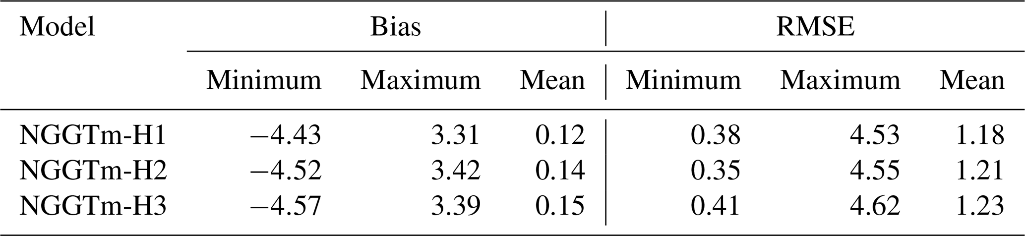
From Table 1, as the resolution of the model increased, the mean bias of the NGGTm-H model gradually decreased. The mean bias of the NGGTm-H1 model was smallest, at 0.12 K. Compared to those of the NGGTm-H2 model and the NGGTm-H3 model, the mean bias of the NGGTm-H1 model was reduced by only 0.02 and 0.03 K, respectively. Positive mean biases with relatively small absolute values were obtained for the NGGTm-H model at the three resolutions taking T_m data from radiosonde stations as reference values. The main reason for these results was that the majority of radiosonde stations are located in land areas. The vertical adjustment values of T_m obtained using the NGGTm-H model were slightly larger in land areas but smaller in marine areas than the reference values. However, a small number of radiosonde stations distributed in marine areas was susceptible to the influence of marine climate, resulting in the vertical adjustment values of the model being apparently smaller than the reference values. Therefore, the positive biases were smaller than the absolute value of the negative biases. In addition, the precision of the NGGTm-H1 model showed the best result with a mean RMSE of 1.18 K. Thus, NGGTm-H1 model had a certain improvement compared to the NGGTm-H2 and NGGTm-H3 models.

4 Development of a global model considering time-varying vertical adjustment rate: NGGTm

4.1 Analysis of T_m temporal characteristics

The NGGTm-H model was described in Sect. 3, it can vertically adjust the given T_m at the surface to the target height. In order to directly obtain T_m at any height, it is necessary to develop a T_m model whose h_bot is at the surface (named as surface T_m model). Analysing the spatiotemporal characteristics of T_m is crucial for developing T_m models. Relevant studies have shown that T_m undergoes diurnal variations (Sun et al., 2019). To further analyse the temporal characteristics in T_m in depth at the global scale, we calculated the annual mean value, annual cycle amplitude, semiannual cycle amplitude, daily cycle amplitude and semidaily cycle amplitude at all grid points using the least-squares adjustment using surface gridded T_m data calculated from all the ERA5 reanalysis data recorded from 2012 to 2016 worldwide. The results are shown in Fig. 5.

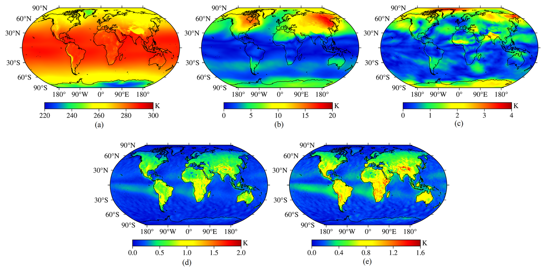
Figure 5 The distributions of the annual mean value and amplitudes of T_m calculated using global ERA5 reanalysis data. (a) Annual mean value. (b) Annual cycle amplitude. (c) Semiannual cycle amplitude. (d) Daily cycle amplitude. (e) Half-day cycle amplitude.

As shown in Fig. 5, strong correlations were found between the annual mean T_m value and latitude and between the annual T_m cycle amplitude and latitude. The semiannual cycle amplitude of T_m also exhibited a certain correlation with latitude, and a certain sea–land difference was observed. In summary, T_m not only undergoes significant annual and semiannual variations but also experiences significant daily and semidiurnal variation.

4.2 Development of the NGGTm model

As mentioned above, it was necessary to consider the time-varying vertical adjustment rate and detailed temporal variations when developing high-precision global T_m models. Therefore, a new global T_m model considering time-varying vertical adjustment rate was developed which used the integrated surface T_m of ERA5 reanalysis recorded from 2012 to 2016 on the basis of NGGTm-H1 model. Because of the significant variations in the horizontal direction of T_m compared to vertical adjustment rate according to Figs. 5a and 3a, it was necessary to develop surface T_m models at each gridded point instead of using sliding windows. This new T_m model is a hybrid-grid model, as the surface T_m model was developed at each gridded point and the NGGTm-H1 model was developed at the geometric centre of the sliding window. The model formulae are expressed as follows:

$$\begin{array}{}\text{(11)}& {\displaystyle }\begin{array}{rl}{T}_{\mathrm{m}}^{\mathrm{G}}=& B_{\mathrm{0}}+B_{\mathrm{1}}\cos \left(\mathrm{2}\mathit{\pi }{\displaystyle \frac{\text{HOD}}{\mathrm{24}}}\right)+B_{\mathrm{2}}\sin \left(\mathrm{2}\mathit{\pi }{\displaystyle \frac{\text{HOD}}{\mathrm{24}}}\right)\\ & +B_{\mathrm{3}}\cos \left(\mathrm{4}\mathit{\pi }{\displaystyle \frac{\text{HOD}}{\mathrm{24}}}\right)+B_{\mathrm{4}}\sin \left(\mathrm{4}\mathit{\pi }{\displaystyle \frac{\text{HOD}}{\mathrm{24}}}\right),\end{array}\text{(12)}& {\displaystyle }\begin{array}{rl}{B}_i=& b_{i\mathrm{0}}+b_{i\mathrm{1}}\cos \left(\mathrm{2}\mathit{\pi }{\displaystyle \frac{\text{DOY}}{\mathrm{365.25}}}\right)+b_{i\mathrm{2}}\sin \left(\mathrm{2}\mathit{\pi }{\displaystyle \frac{\text{DOY}}{\mathrm{365.25}}}\right)\\ & +b_{i\mathrm{3}}\cos \left(\mathrm{4}\mathit{\pi }{\displaystyle \frac{\text{DOY}}{\mathrm{365.25}}}\right)+b_{i\mathrm{4}}\sin \left(\mathrm{4}\mathit{\pi }{\displaystyle \frac{\text{DOY}}{\mathrm{365.25}}}\right)\end{array},\end{array}$$

where $T_{\mathrm{m}}^{\mathrm{G}}$ is the T_m value at the gridded points; B_i is the daily variation coefficient of T_m; HOD is the UTC time. After Eq. (12) was used to expand Eq. (11), b_ij $(i=\mathrm{0},\mathrm{1},\mathrm{2},\mathrm{3},\mathrm{4}$ and $j=\mathrm{0},\mathrm{1},\mathrm{2},\mathrm{3},\mathrm{4}$), which represents the 25 coefficient terms of the model, was calculated. DOY is the day of the year.

The 25 model coefficients were calculated by the least-squares adjustment at all global reanalysis data grid points, which used the surface gridded T_m data with a temporal resolution of 1 h. The above coefficients were stored at the grid points with a horizontal resolution of 0.25°×0.25°. Finally, the NGGTm model considering time-varying vertical adjustment rate was developed. The input parameters for this model are location and time only, which makes it convenient for users. Here, we introduce the use of NGGTm. First, users need to find the window where target points are in, extract the five model coefficients of Eq. (9) for the centre point of the window, and input the DOY to calculate γ. Second, users need to find the four surrounding grid points, extract 100 model coefficients of the surface T_m model (Eqs. 11 and 12) for four grid points, and input HOD and DOY into Eqs. (11) and (12) to calculate the T_m at surface. Then values of T_m at the surface are vertically adjusted to the height of the target point using Eq. (10). Finally, T_m at the target point is obtained using inverse distance-weighted interpolation using the four adjusted T_m.

5 Validation of NGGTm

5.1 Comparison to gridded T_m data

In this section, to validate the accuracy of the new model, The NGGTm model was used to calculate the T_m values at all of the grid points at the global scale, which compared with the Bevis and GPT3 model. The surface gridded T_m data with a temporal resolution of 1 h derived from the ERA5 reanalysis data in 2017 were selected as reference values. We defined the GPT3 model with two horizontal resolutions of 1°×1° and 5°×5° as GPT3-1 and GPT3-5, respectively, which makes it convenient to describe. The T_s data required by the Bevis model to calculate T_m were derived from the GPT3-1 model. The statistical results are listed in Table 2, and shown in Figs. 6 and 7.

Table 2 The precision statistics of the bias and RMSE values of the four models tested using global surface gridded T_m data from the ERA5 reanalysis product in 2017 (unit: k).

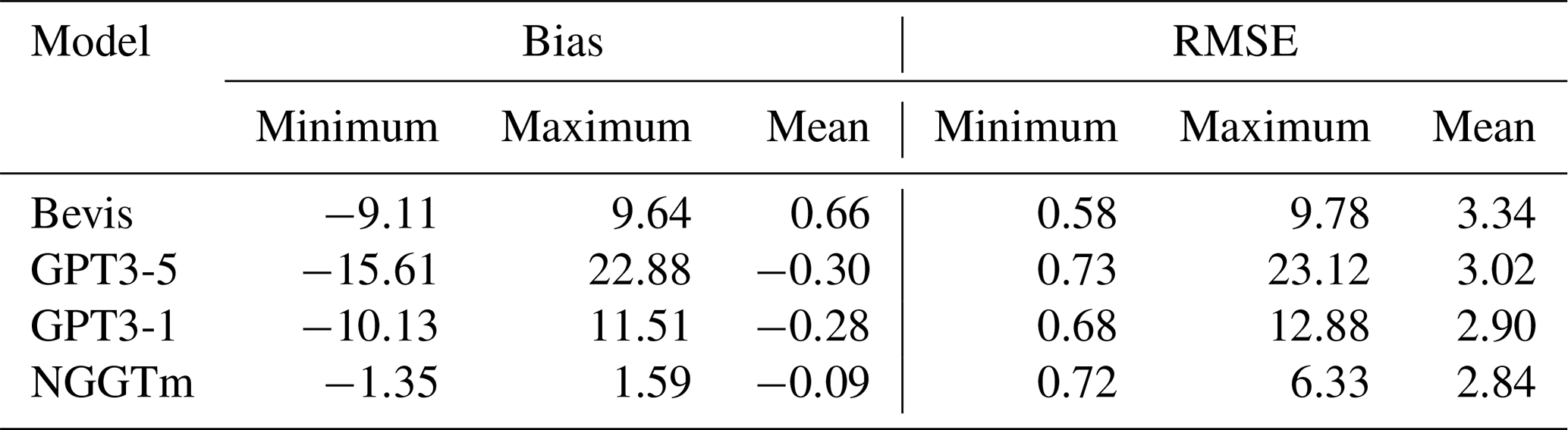
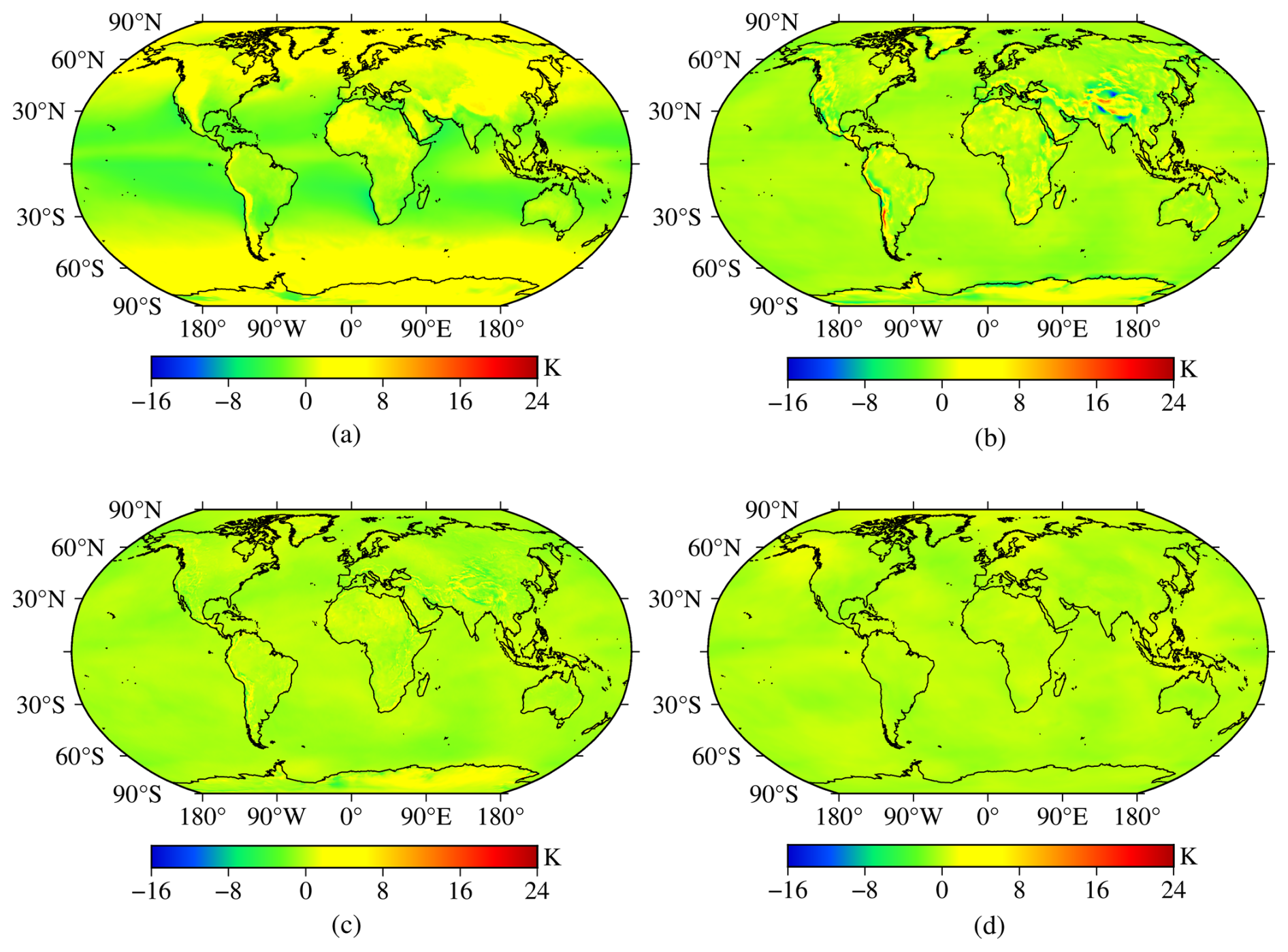
Figure 6 The bias distributions of the four models tested using global surface gridded T_m data from the ERA5 reanalysis product in 2017. (a) Bevis model. (b) GPT3-5 model. (c) GPT3-1 model. (d) NGGTm model.

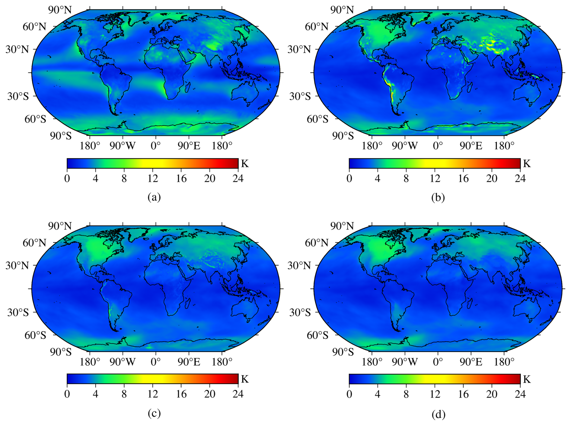
Figure 7 The RMSE distributions of the four models tested using global surface gridded T_m data from the ERA5 reanalysis product in 2017. (a) Bevis model. (b) GPT3-5 model. (c) GPT3-1 model. (d) NGGTm model.

From Table 2, it can be seen that the mean bias of the Bevis model was 0.66 K, which indicated that the T_m values calculated by the Bevis model were all larger than the reference values. The mean biases of the GPT3-5 model and the GPT3-1 model were −0.30 and −0.28 K, respectively, which demonstrated that the T_m values calculated by the GPT3 model were slightly smaller than the reference values. The mean bias of the NGGTm model was only −0.09 K, which was the smallest absolute mean bias value among all the analysed models. This result shows that the T_m values calculated by this model were close to the reference values overall, which demonstrated that the NGGTm model performed better than the other models. In terms of the variation ranges of the bias, the bias variation range of the GPT3-1 model shows improvement compared to that of the GPT3-5 model, which had the largest bias variation range. The main reason for the above results may be that the GPT3 model did not consider the influence of height in its calculation of T_m, which resulted in the relatively large bias in the calculated T_m values in high-elevation areas. The variation range of the bias for the GPT3-1 model was smaller than that of the GPT3-5 model, which indicated that improving the model resolution can help improve the stability of the model. Compared with the Bevis model, GPT3-5 model and GPT3-1 model, the variation range of the bias of the NGGTm model was extremely small, ranging from −1.35 to 1.59 K, which indicated that the stability of the NGGTm model was better than those of the other analysed models. In addition, the mean RMSE of the NGGTm model was only 2.84 K, which exhibited improvements of 0.5, 0.18 and 0.06 K over the Bevis model, the GPT3-5 model and the GPT3-1 model, respectively. These results show that the T_m values calculated by the NGGTm model had the highest precision among all analysed models. In terms of the variation ranges of RMSE, the variation ranges of RMSE for the GPT3-5 model and GPT3-1 model were larger than those of the other models. The RMSE variation range of the GPT3-1 model was smaller than that of the GPT3-5 model. Compared with the other models, the RMSE of the NGGTm model had the smallest variation range, ranging from 0.72 to 6.33 K, which demonstrated that the precision and stability of the NGGTm model were better than those of the other analysed models.

Figure 6 shows that the absolute bias values were relatively small for the Bevis model in the mid-latitude areas. The main reason for this result may be the Bevis model was developed based on radiosonde data in North America. Larger absolute bias values were observed for the GPT3-5 model in relatively high-elevation areas, such as the Qinghai-Tibet Plateau, western South America, and parts of Antarctica. The main reason for this result may be that the GPT3 model did not take any T_m vertical adjustment into account. The absolute bias values of the GPT3-1 model were smaller than those of the GPT3-5 model in most parts of the world. Although relatively large absolute bias values were still shown for the GPT3-1 model in relatively high-elevation areas, a significant improvement can be seen. Therefore, the performance and stability of the model can be significantly improved by increasing the resolution of the model. The bias of the NGGTm model remained at approximately 0 K, significantly better than those of the other models. In conclusion, the NGGTm model shows excellent stability and applicability at the global scale.

From Fig. 7, relatively large RMSEs obtained for the Bevis model are shown in some areas, which indicated that the Bevis model performed poorly in the Qinghai-Tibet Plateau, northeastern Asia, the coasts of western and southwestern Africa, the Arctic Ocean and Antarctica. Relatively large RMSEs obtained for the GPT3-5 model are shown in western North America, western South America and the Qinghai-Tibet Plateau. The GPT3-1 model had a certain accuracy improvement compared with the GPT3-5 model in these areas. Furthermore, increasing the resolution of the model can improve the model precision of calculating T_m. The NGGTm model had small RMSEs around the world, which demonstrated higher precision especially at low latitudes. The NGGTm model performed significantly better than the Bevis model, the GPT3-5 model and GPT3-1 model.

5.2 Comparison to radiosonde data

To further validate the performance of the NGGTm model, the T_m data from 378 radiosonde stations around the world in 2017 were selected as reference values. The precision of the NGGTm model when calculating T_m at these stations was validated and compared with the other three models. The T_s data required by the Bevis model to calculate T_m were derived from the radiosonde stations. The statistical results are listed in Table 3, and shown in Figs. 8 and 9.

Table 3 The precision statistics of bias and RMSE for the four models tested using global T_m data from 378 radiosonde stations in 2017 (unit: k).

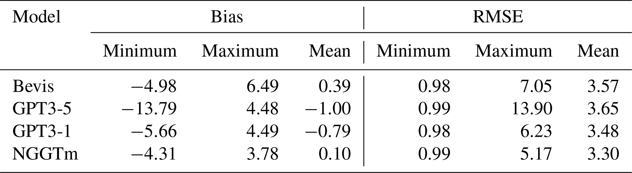
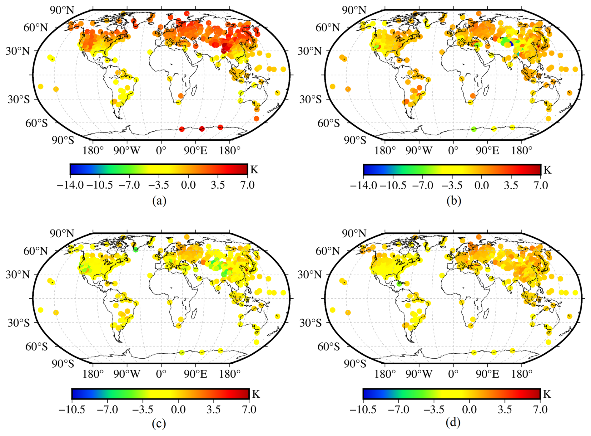
Figure 8 The bias distributions of the four models tested using global T_m data from 378 radiosonde stations in 2017. (a) Bevis model. (b) GPT3-5 model. (c) GPT3-1 model. (d) NGGTm model.

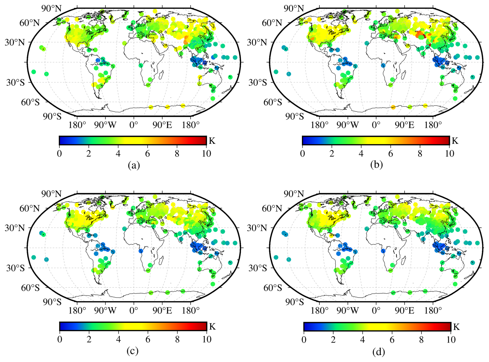
Figure 9 The RMSE distributions of the four models tested using global T_m data from 378 radiosonde stations in 2017. (a) Bevis model. (b) GPT3-5 model. (c) GPT3-1 model. (d) NGGTm model.

From Table 3, the mean bias of the NGGTm model was only 0.10 K, with the smallest absolute value among the analysed models. The bias range of the NGGTm model was also the smallest, ranging from −4.31 to 3.78 K, which demonstrated that the NGGTm model performed better than the other models. In addition, the mean RMSE of the NGGTm model was only 3.30 K, which exhibited improvements of 0.27 K (8 %), 0.35 K (11 %) and 0.18 K (5 %) over the Bevis model, GPT3-5 model and GPT3-1 model, respectively. The RMSE range of the NGGTm model was the smallest, ranging from 0.99 to 5.17 K, indicating that the NGGTm model had the best precision and stability at the global scale.

From Fig. 8, the Bevis model showed relatively obvious negative biases in low latitudes and obvious positive biases in middle and high latitudes, with a trend of increasing absolute biases from low latitudes to high latitudes. The GPT3-5 model and GPT3-1 model performed similarly, with relatively large absolute bias values on the Qinghai-Tibet Plateau and in western North America because the GPT3 model did not consider the relationship between T_m and height. The absolute bias values of the NGGTm model were relatively small at the global scale, with values of approximately 0 K. These results demonstrated that the stability of the NGGTm model was better than those of the other analysed models at the global scale.

Figure 9 shows all models exhibited relatively small RMSEs at low latitudes and relatively large RMSE values at high latitudes, with a trend of increasing RMSEs from low latitudes to high latitudes. The main reason for this result may be the seasonal variation in T_m is strengthened with increasing latitude. In addition, the GPT3-5 model showed relatively large RMSEs at a few radiosonde stations on the Qinghai-Tibet Plateau, whereas the GPT3-1 model exhibited a certain improvement for the reasons mentioned above. The NGGTm model still had a significant improvement compared with other models at the global scale, which demonstrated that the NGGTm model had the best precision and stability.

Since there are strong correlations between T_m and both elevation and latitude, to further analyse the relationship between the precision of T_m calculated by the four models and the elevation variation, the 378 radiosonde stations around the world were divided into five intervals with an elevation span of 500 m for each interval. The bias and RMSE values at these 378 radiosonde stations were then calculated according to the above intervals. The results are shown in Fig. 10.

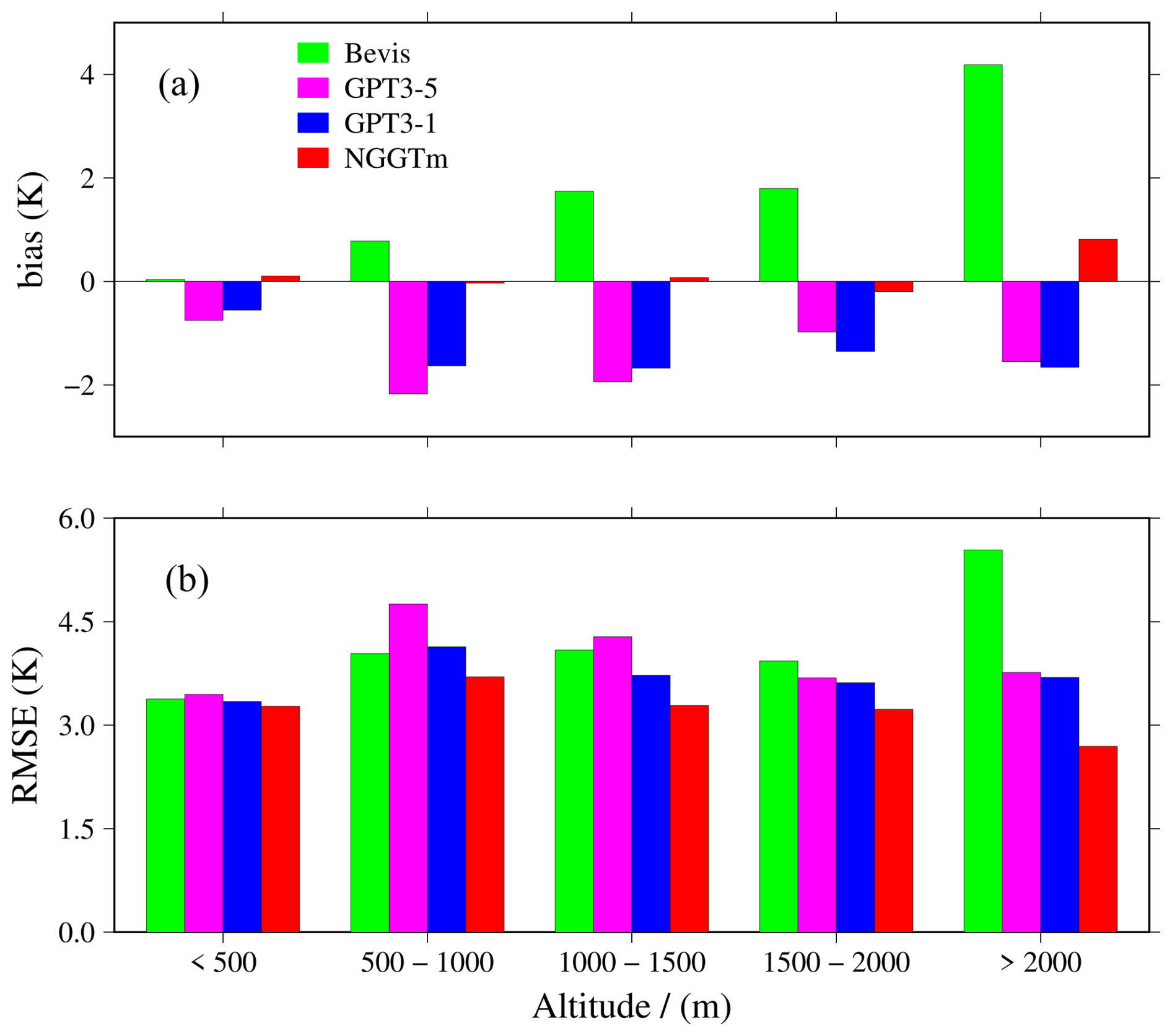
Figure 10 The bias and RMSE distributions within different elevation intervals for the four models tested using global T_m data from 378 radiosonde stations in 2017. (a) Bias. (b) RMSE.

From Fig. 10, the Bevis model exhibited a positive correlation between bias and elevation. The main reason for this result may be that the Bevis model was developed by using radiosonde data collected in low-elevation North America, leading to the poor applicability in relatively high-elevation areas. The GPT3-5 model and GPT3-1 model exhibited negative biases in all elevation intervals. Whereas the NGGTm model exhibited relatively small absolute biases in all elevation intervals, especially those below 2000 m. Therefore, the NGGTm model exhibited extremely significant stability in all elevation intervals compared with other models at the global scale. In addition, the Bevis model showed smaller RMSEs than the GPT3-5 model at elevations below 1500 m. The RMSEs of the GPT3-1 model were smaller than those of the GPT3-5 model at all elevation intervals, which further indicated that increasing the resolution of the model can improve the precision and stability of the results. The RMSEs of the NGGTm model were smaller than those of the Bevis model, GPT3-5 model and GPT3-1 model in all elevation intervals. In conclusion, the NGGTm model showed the best precision and stability compared with the other analysed models in all elevation intervals.

To further analyse the relationship between the precision of four models and the latitude variation, the 378 radiosonde stations around the world were divided into several intervals with a latitude interval of 15°. Few radiosonde stations are located at high latitudes. The high-latitude areas in the Northern and Southern Hemispheres were divided into intervals with latitude intervals of 15°. The bias and RMSE values corresponding to the 378 radiosonde stations were calculated according to the above intervals. The results are shown in Fig. 11.

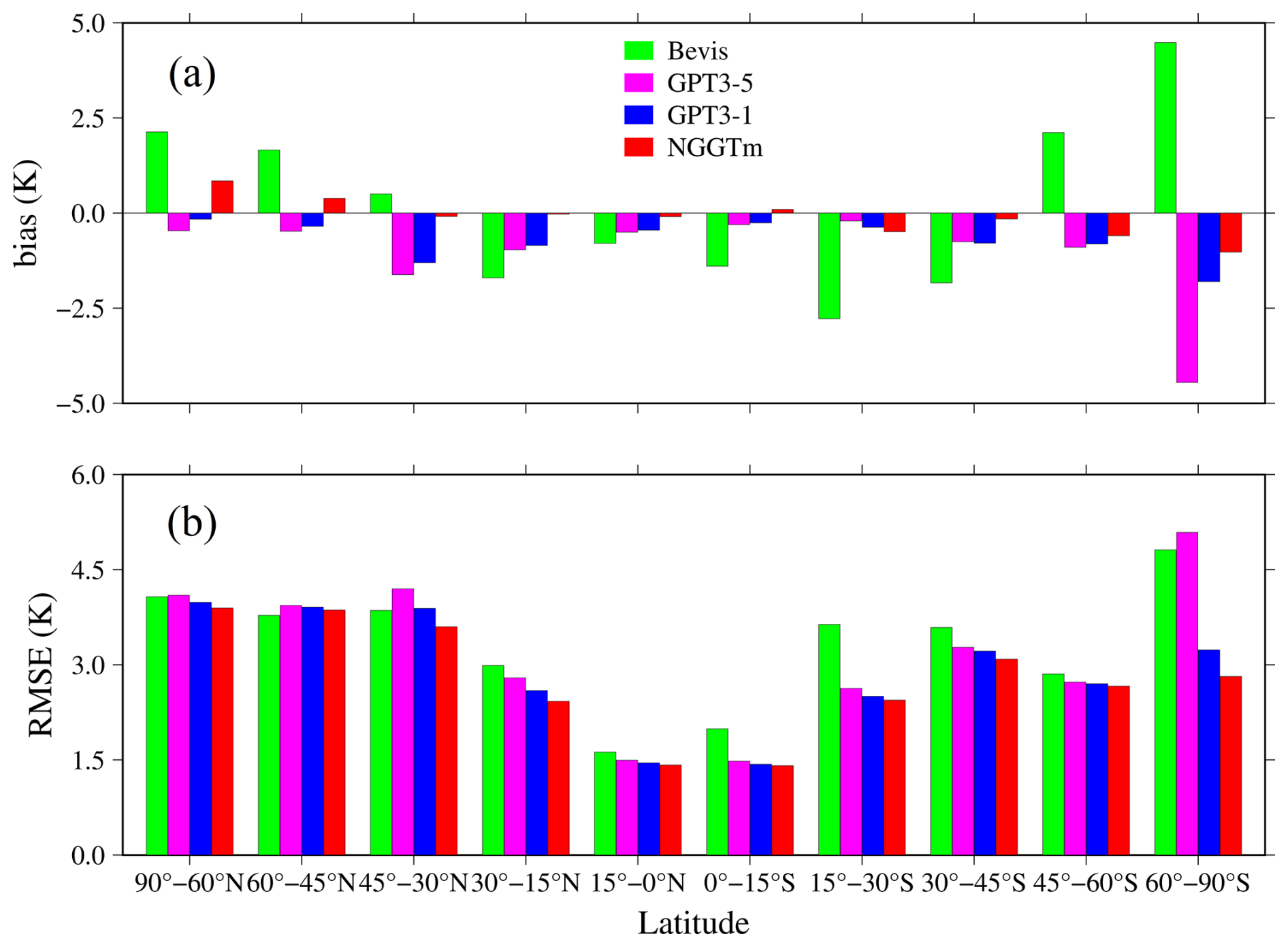
Figure 11 The bias and RMSE distributions in different latitude ranges obtained for the four models tested using T_m data recorded at 378 radiosonde stations globally in 2017. (a) Bias. (b) RMSE.

From Fig. 11, the Bevis model obtained relatively large absolute biases in most latitude ranges, which exhibited significantly positive biases in high latitudes and significantly negative biases in low latitudes. The GPT3-5 and GPT3-1 models exhibited negative biases with relatively small absolute values at most latitudes and negative biases with relatively large absolute values in the high-latitude areas of the Southern Hemisphere, which can be observed especially for the GPT3-5 model. The NGGTm model exhibited small absolute biases in all latitude ranges. In addition, all models showed small RMSEs in low-latitude areas but relatively large RMSEs in high-latitude areas. The RMSEs gradually increased with increasing latitude for all models. Compared to the other models, the NGGTm model had the best accuracy in all latitude ranges, especially in the high-latitude areas of the Southern Hemisphere. In summary, the NGGTm model showed a high accuracy and stability for calculating T_m at all latitudes.

6 Conclusion

T_m is the key parameter of GNSS PWV inversion tasks and in the detection of PWV changes. Developing a real-time and high-precision T_m vertical adjustment rate model is necessary for T_m vertical adjustment. By analysing the relationship between T_m and height, an approximately linear relationship between T_m and height can be found in the near-Earth space. Therefore, a linear function was used to fit the vertical adjustment rate of T_m. Based on an in-depth analysis of the detailed temporal variations in the T_m vertical adjustment rate, a sliding-window algorithm was introduced to develop the NGGTm-H model with horizontal resolutions of 0.5°×0.5°, 1°×1° and 2°×2°. The user can obtain the corresponding vertically adjusted T_m value in real time by providing only the coordinate information of any position and DOY. The NGGTm-H model can achieved excellent results in the precision verification performed by combining ERA5 reanalysis data and radiosonde data that were not used in the modelling process.

Based on the development of the T_m vertical adjustment rate model and taking into account the effects of the detailed temporal characteristics of T_m, NGGTm model was developed. The accuracy and applicability of the NGGTm model were then verified by global radiosonde data and ERA5 reanalysis data that were not used in the modelling process, which compared with those of the Bevis model and GPT3 model. The results show that the NGGTm model had the best performance and stability among the tested models. Compared to the Bevis model and GPT3 model, with increasing height, the performance improvement of the NGGTm model was more significant. The accuracy of the NGGTm model was also significantly improved with increasing latitude. In general, the NGGTm model can provide real-time and high-precision T_m information without requiring the input of measured meteorological parameters at the global scale. This model has broad application prospects in real-time GNSS PWV detection research.

This study only verifies the stability and applicability of the NGGTm model, whereas the model has not yet been applied to GNSS PWV retrieval tasks. Therefore, the effectiveness of the NGGTm model in retrieving atmospheric PWV will be further investigated in future study.