A bound-constrained formulation for complex solution phase minimization

Prediction of mineral phase assemblages is essential to better understand the dynamics of the solid Earth, such as metamorphic processes, magmatism and the formation of mineral ore deposits. While recently developed thermodynamic databases allow the prediction of stable phase mineral assemblages for an increasing range of pressure, temperature and compositional spaces, the increasing complexity of these databases results in a significant increase of computational cost, hindering our ability to perform realistic models of reactive fluid/magma transport. Presently, prediction of stable phase equilibrium in complex systems is therefore largely limited by how efficiently single phase minimization can be performed, as more than 75 % of the total computational time is generally dedicated to individual solution phase minimization. This limitation becomes critical for non-ideal solution phase models that involve both a large number of chemical components, and mixing on a large number of sites, resulting in many inequality constraints of the form $\mathrm{0}\le x_l^M\le \mathrm{1}$, where $x_l^M$ is the fraction of element l mixing on site M.

Here, we present a general reformulation of complex non-ideal solution phases from the thermodynamic database of Holland et al. (2018), which comprises equations of state for multiple mineral solid solutions appearing in magmatic systems, as well as multicomponent silicate melt and aqueous fluid phases. Using a nullspace approach, non-linear inequality constraints governing the site fractions are transformed into equality constraints, and the resulting problem is turned into an bound-constrained optimization problem, subsequently optimized using efficient gradient-based methods. To test our formulation, we apply it to several equations of state for solution phases known for their complexity and compare the results of our approach against classical optimization algorithms supporting inequality constraints.

We find that the the Broyden-Fletcher-Goldfarb-Shanno (BFGS) algorithm yields by far the best performance and stability with respect to the other investigated methods, improving the minimization time of individual solution phase by a factor ≥10. We estimate that our new approach can improve the computational time of stable phase equilibrium by a factor ≥5, thus potentially allowing to model realistic reactive fluid/magmatic systems by directly integrating phase equilibrium calculations in multiphase thermomechanical codes.

1 Introduction

While the last decade has seen significant progress in thermomechanical modeling of complex multiphase systems (e.g., Keller et al., 2013; Taylor-West and Katz, 2015; Keller and Katz, 2016; Keller et al., 2017; Turner et al., 2017; Keller and Suckale, 2019; Rummel et al., 2020; Katz et al., 2022), the coupling with petrological modeling, when addressed at all, remains largely simplified (Riel et al., 2019). There are two key obstacles. First, most phase equilibrium modeling tools (e.g., Perple_X, Theriak_Domino, geoPS, MELTS) (Connolly, 2005; de Capitani and Petrakakis, 2010; Xiang and Connolly, 2021; Ghiorso and Sack, 1995) have been developed with the primary aim of producing phase diagrams and do not offer useful interfaces to integrate with (parallel) geodynamic codes. Second, phase equilibrium modeling is generally achieved by solving a Gibbs energy minimization problem which is computationally challenging. Several numerical strategies have been developed to solve such optimization problems (Ghiorso and Sack, 1995; Connolly, 2005; de Capitani and Petrakakis, 2010; Piro, 2011; Xiang and Connolly, 2021) and some of the most efficient algorithms rely on repeated solution model minimization in order to compute for the most stable mineral assemblage (e.g., de Capitani and Petrakakis, 2010; Xiang and Connolly, 2021; Riel et al., 2022). Although computational performance have been significantly increased over the past few years (Xiang and Connolly, 2021; Riel et al., 2022),single point equilibrium prediction is still costly, with computational times of the order of 10 to 100 ms (e.g., Riel et al., 2022). This limitation effectively precludes direct coupling of phase equilibrium calculations with thermomechanical models, which requires performing from thousands to hundreds of thousands of such calculations every timestep.

In order to account for chemical separation in geodynamic models, several computationally cheaper workarounds have been used. This includes the use of pre-computed set of pseudosections (e.g., Magni et al., 2014; Bouilhol et al., 2015; Rummel et al., 2020), parameterizations (e.g., Jackson et al., 2003, 2018; Hu et al., 2022; Wong and Keller, 2023) and the ongoing development of neural networks (e.g., Leal et al., 2020; Yuan et al., 2024; Candioti et al., 2024). In (Rummel et al., 2020), the authors generated a database of pre-computed results from phase-equilibria modeling covering the explored/expected compositional, pressure and temperature range of the system. While this approach is powerful, it suffers several limitations. First, to generate a relevant petrological database, the geodynamic model has to be run multiple times in order to characterize the effective pressure, temperature and compositional range of the system. Second, the database is by definition discrete which implies that a compositional tolerance has to be applied when computing the stable phase equilibrium, thus leading to mass conservation issues.

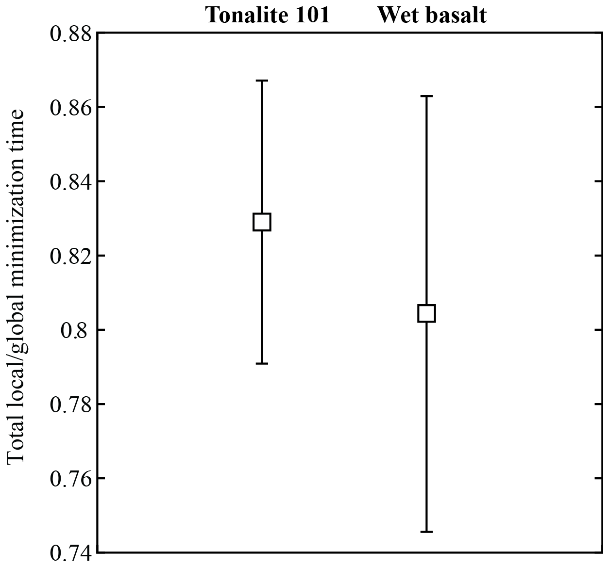
Figure 1 Ratio of time spent solving the local problem of the equilibrium composition and order in individual solution models (“total local”), to time spent solving the entire problem of establishing which is the most stable of the possible phase equilibria (“global minimization”), using MAGEMin (Riel et al., 2022) for two representative test cases. Both tonalite and wet basalt bulk-rock compositions are taken from (Holland et al., 2018). In total 619 points were computed from 0 to 12 kbar and from 600 to 900 °C and from 800 to 1100 °C for the tonalite and the wet basalt case, respectively.

Although the heavy computational requirements of stable phase equilibrium modeling remains a major obstacle for direct coupling, recently developed minimization tools yielded a significant improvement in performance (Xiang and Connolly, 2021; Riel et al., 2022). The recent performance increase mainly results from combining/improving existing minimization methods and making use of gradient-based minimization of individual phases to speed up the computations. Several gradient-based minimization methods are currently employed in the different routines computing phase equilibria. Theriak-Domino (de Capitani and Brown, 1987; de Capitani and Petrakakis, 2010) uses either steepest gradient or Newton-Raphson methods. Minimization of the solution phase model is achieved using a feasible starting guess and continues until a bound or a site fraction constraint is violated. In our recent phase equilibrium calculation software MAGEMin (Riel et al., 2022), the analytical expressions of the equations of state for solution phases are passed to NLopt software package (Johnson, 2021). Subsequently, the objective function is minimized using the Conservative Convex Separable Approximation with Quadratic penalty (CCSAQ) algorithm (Svanberg, 2002) which solves for inequality-constrained nonlinear programming problems. During the inner iterations, a series of convex sub-problems approximating the objective function and the constraints are generated and solved until the constraints are satisfied (Svanberg, 2002). This procedure is repeated until the solution phase model is minimized. The phase equilibria calculator GeoPS (Xiang and Connolly, 2021) uses the simulated annealing (SA) method. Compared to gradient-based methods, simulated-annealing is a probabilistic technique for approximating the global optimum of a given function (e.g., Pincus, 1970). Here, constraints can be accounted for as penalties on the objective function.

The first release of MAGEMin followed the thermocalc software (Powell and Holland, 1988) in treating the physicality of site fractions as a set of inequality constraints expressed as functions of compositional and order variables (Holland et al., 2018) (see e.g., Eq. 11). This approach ensures that all site fractions in the present solution phases satisfy the condition ≥0. Furthermore, since the parameterisation of site fractions enforces that the sum of all site fractions associated with a given site equals unity, this automatically guarantees that all individual site fractions are also ≤1. However, the use of inequality constraint in gradient-based methods, results in relatively slow performances and occasional solver failure due to slight violation of inequality constraints. Using the first publicly released version of MAGEMin (Riel et al., 2022), we find that the global minimization time is largely dominated by how fast gradient-based minimization of individual solution phases can be performed, with 75 % to 90 % of the computation time dedicated to local minimization to find the equilibrium compositions and state of order of solution models (see Fig. 1). Therefore, it becomes critically important to improve the minimization time of individual solution phase models to further speed-up the overall phase-equilibrium computational time.

Here, we present a revised implementation of the compositional and order variables (xeos) of Holland et al. (2018) within MAGEMin that avoids the need to express the site fraction expressions as non-linear inequality constraints. Elimination of these constraints allows using faster bound-constrained optimization methods, thus considerably improving performance and stability of the code. We compare the accuracy and performance of two well-known gradient-based optimization methods: the conjugate gradient (CG) and the Broyden-Fletcher-Goldfarb-Shanno (BFGS) method.

2 Methodology

2.1 Solution phase formulation

At fixed pressure P and temperature T, the total Gibbs energy of solution phase λ is given by

$$\begin{array}{}\text{(1)}& G_{\mathit{\lambda }}=\sum _{i=\mathrm{1}}^{N_{\mathit{\lambda }}}{\mathit{\mu }}_{i\left(\mathit{\lambda }\right)}{p}_{i\left(\mathit{\lambda }\right)}.\end{array}$$

where G_λ [J] is the Gibbs energy of the solution phase λ, N_λ the number of end-members of solution phase λ, p_i(λ) [mol] is the fraction of end-member i dissolved in solution phase λ and μ_i(λ) [J mol⁻¹] is the molar chemical potential of end-member i in solution phase λ. An end-member is defined as an independent instance of a solution phase, at a single specified composition, for which the Gibbs energy is fully defined as a function of pressure and temperature only. In a given chemical system, the linear combinations of the end-members span the complete crystallographic site-occupancy space of the solution phase.

The molar chemical potential of a phase is a function of the dissolved end-members within a solution phase (see Ganguly, 2001 for a review)

$$\begin{array}{}\text{(2)}& {\mathit{\mu }}_{i\left(\mathit{\lambda }\right)}=g_{i\left(\mathit{\lambda }\right)}^{\mathrm{0}}+RT\ln \left(a_{i\left(\mathit{\lambda }\right)}^{\mathrm{id}}\right)+g_{i\left(\mathit{\lambda }\right)}^{\mathrm{ex}},\end{array}$$

where R [J mol⁻¹ K⁻¹] is the ideal gas constant, T [K] is the absolute temperature, $a_{i\left(\mathit{\lambda }\right)}^{\mathrm{id}}$ [/] is the ideal activity, $g_{i\left(\mathit{\lambda }\right)}^{\mathrm{0}}$ [J mol⁻¹] the reference molar Gibbs energy of the pure end-member (Helgeson, 1978; Holland and Powell, 1998) and $g_{i\left(\mathit{\lambda }\right)}^{\mathrm{ex}}$ [J mol⁻¹] is the molar excess energy term (Powell and Holland, 1993; Holland and Powell, 2003). The ideal activity coefficient $a_{i\left(\mathit{\lambda }\right)}^{\mathrm{id}}$ is generally defined as $a_{i\left(\mathit{\lambda }\right)}^{\mathrm{id}}=p_{i\left(\mathit{\lambda }\right)}$ for molecular mixing, or else for mixing on crystallographic sites as

$$\begin{array}{}\text{(3)}& a_{i\left(\mathit{\lambda }\right)}^{\mathrm{id}}=c_i\prod _s(X_{e_{s,i}}^{\mathrm{s}}{)}^{{\mathit{\nu }}_s}\end{array}$$

where $X_{e_{s,i}}^{\mathrm{s}}$ is the site fraction of the element e_s,i that appears on site s in end-member i of phase λ, ν_s is the number of atoms contained in mixing site s of λ, and c_i is a normalization constant that ensures that $a_{i\left(\mathit{\lambda }\right)}^{\mathrm{id}}$ is unity for the pure end-member i.

In the asymmetric formalism, $g_i^{\mathrm{ex}}$ is given by:

$$\begin{array}{}\text{(4)}& \begin{array}{rl}{g}_{i\left(\mathit{\lambda }\right)}^{\mathrm{ex}}& =-\sum _{m=\mathrm{1}}^{N_{\mathit{\lambda }}-\mathrm{1}}\sum _{n>m}^{N_{\mathit{\lambda }}}({\mathit{\varphi }}_m^{\prime }-{\mathit{\varphi }}_m)({\mathit{\varphi }}_n^{\prime }-{\mathit{\varphi }}_n)\\ & \cdot W_{m,n}\left({\displaystyle \frac{\mathrm{2}{v}_i}{v_m+v_n}}\right),\end{array}\end{array}$$

where ϕ_m,n is the proportion of end-members m,n weighted by the asymmetry parameters, as ${\mathit{\varphi }}_{m,n}=\left(p_{m,n}{v}_{m,n}\right)/\left({\sum }_{k=\mathrm{1}}^{N_{\mathit{\lambda }}}{p}_k{v}_k\right)$, with $v_{m,n,k}$ the van Laar parameters for end-members $m,n,k$. ${\mathit{\varphi }}_{m,n}^{\prime }=\mathrm{1}$ where m=n and ${\mathit{\varphi }}_{m,n}^{\prime }=\mathrm{0}$ where m≠n. W_m,n [J mol⁻¹] is the interaction energy between end-members m and n in the solution.

In Holland et al. (2018), composition (the overall ratios of elements) and order (the distribution of elements over mixing sites) in an xeos are parameterized in terms of an independent set of variables (see example below). Given this formulation, the set of Eqs. (1) to (4) can be directly transformed into the following Gibbs free energy minimization problem as function of the compositional and order variable x_cv:

$$\begin{array}{}\text{(5)}& \min G_{\mathit{\lambda }}\left({\mathit{x}}_{\mathrm{cv}}\right)=\sum _{i=\mathrm{1}}^{N_{\mathit{\lambda }}}{\mathit{\mu }}_{i\left(\mathit{\lambda }\right)}{p}_{i\left(\mathit{\lambda }\right)},\end{array}$$

subject to the site fraction of the element

$$\begin{array}{}\text{(6)}& X_{e_{s,i}}^{\mathrm{s}}\ge \mathrm{0},\end{array}$$

and that the compositional and order variables x_cv must be within a lower (lb_cv) and upper (ub_cv) limit

$$\begin{array}{}\text{(7)}& \mathit{l}{\mathit{b}}_{\mathrm{cv}}\le {\mathit{x}}_{\mathrm{cv}}\le \mathit{u}{\mathit{b}}_{\mathrm{cv}},\end{array}$$

where μ_i(λ), p_i(λ), and $X_{e_{s,i}}^{\mathrm{s}}$ are functions of the compositional and order variables x_cv, and, lb_cv and ub_cv are the lower and upper bounds on the set of compositional and order variables x_cv. The first derivative of f(x_cv) is given by

$$\begin{array}{}\text{(8)}& {\displaystyle \frac{\partial f}{\partial {\mathit{x}}_{\mathrm{cv}}}}={\mathit{\mu }}_{i\left(\mathit{\lambda }\right)}{\displaystyle \frac{\partial p_{i\left(\mathit{\lambda }\right)}}{\partial {\mathit{x}}_{\mathrm{cv}}}},\end{array}$$

and the first derivative of the inequality constraints on the site fraction by

$$\begin{array}{}\text{(9)}& {\displaystyle \frac{\partial X_{e_{s,i}}^{\mathrm{s}}}{\partial {\mathit{x}}_{\mathrm{cv}}}}.\end{array}$$

2.2 A revised formulation

The solid solutions presented in Holland et al. (2018) are formulated on the basis of exchanging chemical species on a finite number of unique crystallographic sites (Bragg–Williams-type formulation, see Myhill and Connolly, 2021 for more details). A key challenge with this formulation is that minimization has to be performed while keeping site fractions ≥0. Our previous implementation (Riel et al., 2022) imposed these inequalities constraints directly using NLopt (Johnson, 2021), which has a significantly higher numerical cost compared to the bound-constrained minimization algorithms. To simplify the optimization problem and reduce computation time, we use an alternative nullspace formulation (similar to HeFESTo, Stixrude and Lithgow-Bertelloni, 2011), different from the compositional and order variable approach used in e.g., Holland et al. (2018), that transforms the non-linear inequality constraints on the site fractions into linear equality constraints. This reformulation is illustrated below using olivine as a representative example.

The olivine solid solution model (Holland et al., 2018) contains 2 mixing sites M1 and M2 and represents a phase that can be expressed by the general formula:

$$\begin{array}{}\text{(10)}& [{\mathrm{Mg}}^{\mathrm{2}+},{\mathrm{Fe}}^{\mathrm{2}+}{]}^{\mathrm{M}\mathrm{1}}[{\mathrm{Mg}}^{\mathrm{2}+},{\mathrm{Fe}}^{\mathrm{2}+},{\mathrm{Ca}}^{\mathrm{2}+}{]}_{\mathrm{4}}^{\mathrm{M}\mathrm{2}\mathrm{SiO}}\end{array}$$

Here Mg²⁺ and Fe²⁺ can be exchanged on crystallographic site M1 and Mg²⁺, Fe²⁺ and Ca²⁺ can be exchanged on site crystallographic M2. In Holland et al. (2018), the site fractions are expressed as:

$$\begin{array}{}\text{(11)}& {\displaystyle }{X}_{\mathrm{Mg}}^{\mathrm{M}\mathrm{1}}=\mathrm{1}-x+Q\text{(12)}& {\displaystyle }{X}_{\mathrm{Fe}}^{\mathrm{M}\mathrm{1}}=x-Q\text{(13)}& {\displaystyle }{X}_{\mathrm{Mg}}^{\mathrm{M}\mathrm{2}}=(\mathrm{1}-x)(\mathrm{1}-c)-Q\text{(14)}& {\displaystyle }{X}_{\mathrm{Fe}}^{\mathrm{M}\mathrm{2}}=x(\mathrm{1}-c)+Q\text{(15)}& {\displaystyle }{X}_{\mathrm{Ca}}^{\mathrm{M}\mathrm{2}}=c\end{array}$$

where composition has been parameterized using the variables $x=(X_{\mathrm{Fe}}^{\mathrm{M}\mathrm{1}}+X_{\mathrm{Fe}}^{\mathrm{M}\mathrm{2}})/(X_{\mathrm{Fe}}^{\mathrm{M}\mathrm{1}}+X_{\mathrm{Fe}}^{\mathrm{M}\mathrm{2}}+X_{\mathrm{Mg}}^{\mathrm{M}\mathrm{1}}+X_{\mathrm{Mg}}^{\mathrm{M}\mathrm{2}})$ and $c=X_{\mathrm{Ca}}^{\mathrm{M}\mathrm{2}}$, and order has been parameterized using the variable $Q=x-\left(X_{\mathrm{Fe}}^{\mathrm{M}\mathrm{1}}\right)/(X_{\mathrm{Fe}}^{\mathrm{M}\mathrm{1}}+X_{\mathrm{Mg}}^{\mathrm{M}\mathrm{1}})$. Note that we have dropped the ion charges in the notation of the equations.

This parameterisation ensures that the site fractions on each of the individual sites are inherently normalized to 1. Two other types of constraint might be built into the parameterisation in a more complex example: (i) charge balance: if variably-charged ions were mixing, charge balance would be maintained during compositional change, and (ii) equidistribution: the xeos might be simplified by equating two site fractions, typically involving minor elements. The resulting set of composition and order variables is an independent set, that fully and uniquely describes the site occupancies at a given composition and state of order, subject to physical constraints arising from the lattice structure of the mineral. The relationship between the number of composition and order variables and the number of site fractions is then given by:

$$\begin{array}{}\text{(16)}& n_{\mathrm{sf}}=n_{x_{\mathrm{cv}}}+n_{{\mathrm{eq}}_{\mathrm{norm}}}+n_{{\mathrm{eq}}_{\mathrm{cb}}}+n_{{\mathrm{eq}}_{\mathrm{edist}}},\end{array}$$

with n_sf the number of site fractions, $n_{x_{\mathrm{cv}}}$ the number of compositional and order variables, $n_{{\mathrm{eq}}_{\mathrm{norm}}}$ the number of constraints arising from the normalization of site fractions on a given site to 1, $n_{{\mathrm{eq}}_{\mathrm{cb}}}$ the number of charge balance equations, equal to 0 or 1, and $n_{{\mathrm{eq}}_{\mathrm{edist}}}$ the number of equidistribution constraints imposed. Collectively, the normalized charge balance and equidistribution constraints form a set of linear equalities among the site fractions.

In the revised implementation, we retrieve the set of equality constraints Ax=b for olivine from the site fractions ${\mathbf{\text{X}}}_{e_s}^{\mathrm{s}}=\mathit{\{}{X}_{\mathrm{Mg}}^{\mathrm{M}\mathrm{1}},X_{\mathrm{Fe}}^{\mathrm{M}\mathrm{1}},X_{\mathrm{Mg}}^{\mathrm{M}\mathrm{2}},X_{\mathrm{Fe}}^{\mathrm{M}\mathrm{2}},X_{\mathrm{Ca}}^{\mathrm{M}\mathrm{2}}\mathit{\}}$, and compositional and order variables ${\mathit{x}}_{\mathrm{cv}}=\mathit{\{}x,c,Q\mathit{\}}$ as follows. We first take the partial derivatives of site fractions as functions of the compositional and order variables as:

$$\begin{array}{}\text{(17)}& {\displaystyle \frac{\partial {\mathbf{\text{X}}}_{e_{s,i}}^{\mathrm{s}}}{\partial {\mathit{x}}_{\mathrm{cv}}}}=\left[\begin{array}{ccc}-\mathrm{1}& \mathrm{0}& \mathrm{1}\\ \mathrm{1}& \mathrm{0}& -\mathrm{1}\\ c-\mathrm{1}& x-\mathrm{1}& -\mathrm{1}\\ \mathrm{1}-c& -x& \mathrm{1}\\ \mathrm{0}& \mathrm{1}& \mathrm{0}\end{array}\right],\end{array}$$

where ${\mathbf{\text{X}}}_{e_{s,i}}^{\mathrm{s}}$ is the site fraction of the element e_s,i that appears on site s, x_cv the set of compositional and order variables cv and x, c the compositional and order variables of olivine as defined in Holland et al. (2018). Next, we compute the matrix of site mixing coefficients A using symbolic expressions as

$$\begin{array}{}\text{(18)}& \mathbf{\text{A}}=\mathrm{Null}\left(\right({\displaystyle \frac{\partial {\mathbf{\text{X}}}_e}{\partial {\mathit{x}}_{\mathrm{cv}}}}{)}^T)=\left[\begin{array}{ccccc}\mathrm{1}& \mathrm{1}& \mathrm{0}& \mathrm{0}& \mathrm{0}\\ \mathrm{0}& \mathrm{0}& \mathrm{1}& \mathrm{1}& \mathrm{1}\end{array}\right],\end{array}$$

where Null stands for the null space. We then establish the vector of constraints b as

$$\begin{array}{}\text{(19)}& \mathit{b}=\mathit{\{}\mathrm{1},\mathrm{1}\mathit{\}},\end{array}$$

which ensures that the sum of the site fractions of mixing sites X^M1 and X^M2 equal unity. Subsequently, given $\mathit{x}={\mathbf{\text{X}}}_{e_s}^{\mathrm{s}}$ and by linearizing Ax=b we can return the set of linear equalities on the olivine site fractions, which comprises two site normalization expressions:

$$\begin{array}{}\text{(20)}& \mathrm{1}\times X_{\mathrm{Mg}}^{\mathrm{M}\mathrm{1}}+\mathrm{1}\times X_{\mathrm{Fe}}^{\mathrm{M}\mathrm{1}}=\mathrm{1.0},\end{array}$$

and

$$\begin{array}{}\text{(21)}& \mathrm{1}\times X_{\mathrm{Mg}}^{\mathrm{M}\mathrm{2}}+\mathrm{1}\times X_{\mathrm{Fe}}^{\mathrm{M}\mathrm{2}}+\mathrm{1}\times X_{\mathrm{Ca}}^{\mathrm{M}\mathrm{2}}=\mathrm{1.0}.\end{array}$$

Note that, for more complex activity-composition models, and depending on the arbitrary order in which the site fractions are listed, the nullspace operation may not yield expressions that clearly represent the site normalization, charge balance, and equidistribution constraints. However, it will always produce an independent set of linear equalities whose total number is equal to the sum of the number of site normalization constraints, the number of charge balance constraints, and the number of equidistribution constraints. These equalities are mathematically equivalent to the original constraints and can be linearly recombined to recover their straightforward forms.

In the implementation of Riel et al. (2022), MAGEMin solved for the equilibrium composition and state of order of a phase in terms of the variables x_cv, subject to the constraint that the values of site fractions should be ≥0. To eliminate the site fraction inequalities from the implementation, we now wish to solve directly for the site fractions, while subjecting them to the equality constraints obtained via the nullspace operation. The resulting problem can be expressed as

$$\begin{array}{}\text{(22)}& \min f\left(\mathit{x}\right),\end{array}$$

subject to

$$\begin{array}{}\text{(23)}& \mathbf{A}\mathit{x}=\mathit{b},\end{array}$$

where x represent the n site-fractions and Ax=b is the set of p equality constraints (Eq. 18). The linear equality constraints can now be eliminated from the problem, reducing the number of variables solved for back to the number of composition and ordering variables. This is accomplished by parameterizing the feasible set of the constraint equation Ax=b using a particular solution $\widehat{\mathit{x}}\in {\mathbb{R}}^n$ and a matrix $\mathbf{N}\mathit{z}\in {\mathbb{R}}^{n\times (n-p)}$ that spans the nullspace of A, such that:

$$\begin{array}{}\text{(24)}& \mathit{\left\{}\mathit{x}\right|\mathbf{A}\mathit{x}=\mathit{b}\mathit{\}}=\mathit{\{}\widehat{\mathit{x}}+\mathbf{N}\mathit{z}|\mathit{z}\in {\mathbb{R}}^{n-p}\mathit{\}}.\end{array}$$

This parameterization can be obtained by performing a full QR decomposition of the constraint matrix A, written as:

$$\begin{array}{}\text{(25)}& \mathbf{A}=\mathbf{Q}\left[\begin{array}{c}{\mathbf{R}}_{\mathrm{1}}\\ \mathbf{0}\end{array}\right]=\left[\begin{array}{c}{\mathbf{Q}}_{\mathrm{1}}{\mathbf{Q}}_{\mathrm{2}}\end{array}\right]\left[\begin{array}{c}{\mathbf{R}}_{\mathrm{1}}\\ \mathbf{0}\end{array}\right],\end{array}$$

where $\mathbf{Q}\in {\mathbb{R}}^{m\times m}$ is an orthogonal matrix whose columns ${\mathit{q}}_{\mathrm{1}},\mathrm{\dots },{\mathit{q}}_m$ form an orthonormal basis for ℝ^m. These columns are typically grouped into two blocks: Q₁, which contains the first p columns and spans the image (row space) of A, and Q₂, which contains the remaining m−p columns and spans the nullspace of A^T. With this decomposition, the set of solutions to the linear equality constraints can be written as:

$$\begin{array}{}\text{(26)}& \mathit{x}={\mathbf{Q}}_{\mathrm{1}}{\mathbf{R}}_{\mathrm{1}}^T\mathit{b}+{\mathbf{Q}}_{\mathrm{2}}z,\end{array}$$

where $\widehat{\mathit{x}}={\mathbf{Q}}_{\mathrm{1}}{\mathbf{R}}_{\mathrm{1}}^T\mathbf{b}$ is a particular solution to Ax=b, and Q₂z is any vector in the nullspace of A.

In other words, the use of the null space of A (Nz) parameterizes the space such that for any step Δz, $\widehat{\mathit{x}}+\mathbf{N}\mathit{z}\mathrm{\Delta }z$ remains in the feasible domain.

Using the elimination method, Eq. (1) becomes

$$\begin{array}{}\text{(27)}& \min f\left(\mathit{x}\right)=G_{\mathit{\lambda }}\left({\mathbf{X}}_{e_{s,i}}^{\mathrm{s}}\right)=\sum _{i=\mathrm{1}}^{N_{\mathit{\lambda }}}{\mathit{\mu }}_{i\left(\mathit{\lambda }\right)}{p}_{i\left(\mathit{\lambda }\right)},\end{array}$$

and the parameterized first derivative becomes

$$\begin{array}{}\text{(28)}& {\displaystyle \frac{\partial f}{\partial \mathit{x}}}\left(\mathit{z}\right)={\displaystyle \frac{\partial G_{\mathit{\lambda }}}{\partial {\mathbf{X}}_{e_{s,i}}^{\mathrm{s}}}}\left(\mathit{z}\right)={\mathbf{N}}_z\left(\right({\displaystyle \frac{\partial G_{\mathit{\lambda }}}{\partial \mathit{x}}}{)}^T{\mathbf{N}}_z{)}^T,\end{array}$$

where ${\mathbf{X}}_{e_{s,i}}^{\mathrm{s}}$ is the site fraction of the element e_s,i that appears on site s. Equation (27) is then minimized using the gradient information given by Eq. (28) and the methods presented below.

2.3 Gradient-type iterative methods

Given a bound-constrained optimization problem:

$$\begin{array}{}\text{(29)}& \begin{array}{rl}{\displaystyle }min& {\displaystyle }f\left(\mathit{x}\right)\\ {\displaystyle }\text{subject to }& {\displaystyle }\mathit{x}>\mathit{ϵ}\end{array}\end{array}$$

where f(x) is twice continuously differentiable, where ϵ is a small number, typically $\le {\mathrm{10}}^{-\mathrm{8}}$. The general gradient-type iterative method to solve this problem is of the form

$$\begin{array}{}\text{(30)}& {\mathit{x}}_{k+\mathrm{1}}={\mathit{x}}_k+{\mathit{\alpha }}_k{\mathit{d}}_k,\end{array}$$

for iteration k≥0, where d_k is the search direction and α_k is the step-length. In this study, we compute the step-length using a Wolfe line search (Wolfe, 1969) such that the inequalities

$$\begin{array}{}\text{(31)}& f({\mathit{x}}_k+{\mathit{\gamma }}_k{\mathit{\alpha }}_k{\mathit{d}}_k)\le f\left({\mathit{x}}_k\right)+\mathit{\rho }{\mathit{\gamma }}_k{\mathit{\alpha }}_k{\mathit{g}}_k^T{\mathit{d}}_k,\end{array}$$

and

$$\begin{array}{}\text{(32)}& {\mathit{g}}_{k+\mathrm{1}}^T{\mathit{d}}_k\ge \mathit{\sigma }{\mathit{g}}_k^T{\mathit{d}}_k,\end{array}$$

are satisfied, where $\mathrm{0}<\mathit{\rho }<\mathit{\sigma }<\mathrm{1}$ and γ_x is the maximum feasible step-length, computed as

$$\begin{array}{}\text{(33)}& {\mathit{\gamma }}_x=\left\{\begin{array}{ll}\mathrm{1}/\frac{\min ({\mathit{x}}_{k+\mathrm{1}}-\mathit{ϵ})}{\mathrm{abs}\left({\mathit{d}}_k\right)},& \text{if any }{\mathit{x}}_k+{\mathit{d}}_k\le \mathrm{0}\\ \mathrm{1},& \text{otherwise}.\end{array}\right.\end{array}$$

The maximum feasible step-length γ_x ensures that the values of site-fractions remain ≥ϵ and form the bounds of the problem. Iterations are then processed until a stopping criterion is satisfied. Because solution phases are not necessarily convex during global Gibbs energy minimization, we set the stopping criteria using the relative change of the objective function. The stopping criteria is met when

$$\begin{array}{}\text{(34)}& \mathrm{abs}\left(\right(f_k-f_{k-\mathrm{1}})/f_{k-\mathrm{1}})<\mathrm{tol},\end{array}$$

where tol is a small number typically $\le {\mathrm{10}}^{-\mathrm{8}}$.

If the descent direction d_k is simply chosen to be ${\mathit{d}}_k=-{\mathit{g}}_k$ we obtain the steepest descent algorithm. However, this approach is known to be prone to oscillation (e.g., Nocedal et al., 2002) and slow convergence, and will therefore not be explored. Instead, we test two bound-constrained optimization methods that use the gradient information of the previous iteration(s), namely the conjugate gradient and the Broyden-Fletcher-Goldfarb-Shanno (BFGS) method.

2.3.1 Conjugate gradient method

For the conjugate gradient method, the descent direction is initialized for the first iteration increment k=0 as

$$\begin{array}{}\text{(35)}& {\mathit{d}}_k=-{\mathit{g}}_k,\end{array}$$

and for increment k≥1 as

$$\begin{array}{}\text{(36)}& {\mathit{d}}_k=-{\mathit{g}}_k+{\mathit{\beta }}_k{\mathit{d}}_{k-\mathrm{1}}.\end{array}$$

Here, g_k is the gradient g(x) of function f(x) at point x_k, and β_k is the conjugate gradient update parameter. Variants of the conjugate gradient method are defined by using different update parameters β_k (see for example Hestenes and Stiefel, 1952; Rivaie et al., 2012, 2015). Here, we employ the three-term conjugate gradient method presented by Liu et al. (2018) with the update parameter β_k defined in Rivaie et al. (2015)

$$\begin{array}{}\text{(37)}& {\mathit{\beta }}_k={\displaystyle \frac{{\mathit{g}}_k^T({\mathit{g}}_k-{\mathit{g}}_{k-\mathrm{1}}-{\mathit{d}}_{k-\mathrm{1}})}{\Vert {\mathit{d}}_{k-\mathrm{1}}{\Vert }^{\mathrm{2}}}},\end{array}$$

and further extend the descent direction term as

$$\begin{array}{}\text{(38)}& {\mathit{d}}_k=-{\mathit{g}}_k+{\mathit{\beta }}_k{\mathit{d}}_{k-\mathrm{1}}+{\mathit{\theta }}_k{\mathit{y}}_{k-\mathrm{1}},\end{array}$$

where ${\mathit{y}}_{k-\mathrm{1}}={\mathit{g}}_k-{\mathit{g}}_{k-\mathrm{1}}$ and

$$\begin{array}{}\text{(39)}& {\mathit{\theta }}_k=-{\displaystyle \frac{{\mathit{g}}_k^T{\mathit{d}}_{k-\mathrm{1}}}{\Vert {\mathit{d}}_{k-\mathrm{1}}{\Vert }^{\mathrm{2}}}}.\end{array}$$

A useful property of the three-term conjugate gradient method is that the search direction always satisfies the sufficient descent condition without any line search (Liu et al., 2018).

The descent direction is parameterized to satisfy the equality constraints (Eq. 18) such as

$$\begin{array}{}\text{(40)}& {\mathit{d}}_k^p={\mathbf{N}}_z({\mathit{d}}_k^T{\mathbf{N}}_z{)}^T.\end{array}$$

2.3.2 BFGS method

The Broyden-Fletcher-Goldfarb-Shanno (BFGS) method is a well-known quasi-Newton method for solving unconstrained and bound-constrained optimization problems (see for instance Fletcher, 1987; Dennis and Schnabel, 1996). The quasi-Newton descent direction is given by

$$\begin{array}{}\text{(41)}& {\mathit{d}}_k=-{\mathbf{B}}^{-\mathrm{1}}{\mathit{g}}_k,\end{array}$$

where B⁻¹ is the inverse of the Hessian matrix. Here, we approximate B⁻¹ using the Sherman-Morrison formula (Sherman and Morrison, 1950) such as

$$\begin{array}{}\text{(42)}& \begin{array}{rl}{\mathbf{B}}_{k+\mathrm{1}}^{-\mathrm{1}}& ={\mathbf{B}}_k^{-\mathrm{1}}+{\displaystyle \frac{({\mathit{s}}_k^T{\mathit{y}}_k+{\mathit{y}}_k^T{\mathbf{B}}_k^{-\mathrm{1}}{\mathit{y}}_k)\left({\mathit{s}}_k{\mathit{s}}_k^T\right)}{({\mathit{s}}_k^T{\mathit{y}}_k{)}^{\mathrm{2}}}}\\ & -{\displaystyle \frac{{\mathbf{B}}_k^{-\mathrm{1}}{\mathit{y}}_k{\mathit{s}}_k^T+{\mathit{s}}_k{\mathit{y}}_k^T{\mathbf{B}}_k^{-}\mathrm{1}}{{\mathit{s}}_k^T{\mathit{y}}_k}}\end{array}\end{array}$$

where ${\mathit{s}}_k={\mathit{x}}_{k+\mathrm{1}}-{\mathit{x}}_k$, ${\mathit{y}}_k={\mathit{g}}_{k+\mathrm{1}}-{\mathit{g}}_k$ and ${\mathbf{B}}_{k=\mathrm{0}}^{-\mathrm{1}}$ is initialized with the identity matrix.

Because of the relatively low dimensionality of the solution phase model (<20) we do not consider the limited-memory BFGS method (L-BFGS) and instead update ${\mathbf{B}}_k^{-\mathrm{1}}$ (Eq. 42) during every iteration. Once the problem has converged (i.e., Eq. 34 is satisfied), we reset the Hessian matrix inverse ${\mathbf{B}}_{k^{-\mathrm{1}}}$ to the identity matrix and perform additional iteration(s). This ensures that the problem converges to its local minimum in the event the quality of the approximate Hessian matrix inverse ${\mathbf{B}}_{k^{-\mathrm{1}}}$ is degraded.

As for the conjugate gradient method, the descent direction is parameterized to satisfy the equality constraints (Eq. 18) such as

$$\begin{array}{}\text{(43)}& {\mathit{d}}_k^p={\mathbf{N}}_z({\mathit{d}}_k^T{\mathbf{N}}_z{)}^T.\end{array}$$

3 Application

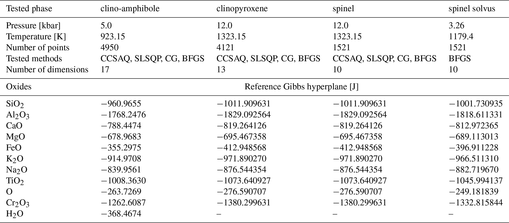
In order to test the bound-constrained solution phase formulation, we selected, from the Holland et al. (2018) set of xeos spaning 11 oxides (Na₂O-CaO-K₂O-FeO-MgO-Al₂O₃-SiO₂-H₂O-TiO₂-O-Cr₂O₃), three solution phases with complex features including high-dimensional composition–order spaces and geologically significant solvi: clinoamphibole (Na₂O-CaO-K₂O-FeO-MgO-Al₂O₃-SiO₂-H₂O-TiO₂-O), clinopyroxene (Na₂O-CaO-K₂O-FeO-MgO-Al₂O₃-SiO₂-TiO₂-O-Cr₂O₃) and spinel (FeO-MgO-Al₂O₃-TiO₂-O-Cr₂O₃) (Table 1). We use as starting points the set of feasible points of each discretized solution phase. Discretization of the solution phases is achieved using a compositional variable step of 0.25 which yielded 5498, 4124 and 1521 feasible starting points (or pseudocompounds) for clino-amphibole, clinopyroxene and spinel, respectively. Because gradient-based minimization of solution phase models is achieved with respect to a given Gibbs hyperplane (de Capitani and Brown, 1987; de Capitani and Petrakakis, 2010; Xiang and Connolly, 2021; Riel et al., 2022), we first compute the phase equilibrium at a given pressure, temperature and bulk-rock composition to retrieve the global minimum Gibbs hyperplane using MAGEMin (Table 1). Although any other arbitrary Gibbs hyperplane can be used for this test, we choose a global minimum hyperplane in order to explore a known spinel solvus, All computations were performed on a Linux (x86_64-linux-gnu) operating system, utilizing a 6-core 11th Gen Intel(R) Core(TM) i5-11400H CPU running at 2.70 GHz.

Table 1 Solution phase models parameters.

The performance and reliability of the bound-constrained formulations are tested against the inequality constrained formulations using the Sequential Least-Squares Quadratic Programming (SLSQP) (Kraft, 1988, 1994) and Conservative Convex Separable Approximation with Quadratic penalty (CCSAQ) methods (Svanberg, 2002). The minimizations using the SLSQP and CCSAQ methods were computed using the C implementation of NLopt (Jackson et al., 2018) through MAGEMin as described in Riel et al. (2022) and in the scripts provided in Supplement. Because the algorithms explored in this study (Julia implementation of CG and BFGS methods) exhibited similar accuracy with residual $\le {\mathrm{10}}^{-\mathrm{13}}$, the differences in algorithm accuracy are not discussed. Here, a minimization is considered successful when the norm of the distance to the solution is $\le {\mathrm{10}}^{-\mathrm{4}}$.

4 Discussion

4.1 Algorithms performance and reliability

The box plots depicted in Fig. 2 illustrate that the performance of the unconstrained CG method is comparable to that of the inequality-constrained CCSAQ method (implemented via NLopt). While the CG method outperforms CCSAQ for amphibole, with minimization times of ∼ 2100 µs versus ∼ 4200 µs, respectively, the efficiency of CCSAQ is larger for problems with lower dimensionality, such as clinopyroxene and spinel. The SLSQP method demonstrates superior efficiency, with average minimization times of ∼ 340 µs for amphibole, ∼ 270 µs for clinopyroxene, and ∼ 120 µs for spinel. However, the BFGS algorithm outperforms SLSQP, achieving average minimization times of ∼ 220 µs for amphibole, 180 µs for clinopyroxene, and ∼ 100 µs for spinel; a performance increase of 20 % to 50 %. Additionally, the BFGS method's convergence requires between 25 to 90 iterations across different solution phase models, as indicated in Fig. 3. Notably, the minimum time per iteration is influenced by the dimensionality of the solution phase model, ranging from ∼ 4.0 µs per iteration for clino-amphibole to ∼ 2.1 µs for spinel (Fig. 3 and Table 1).

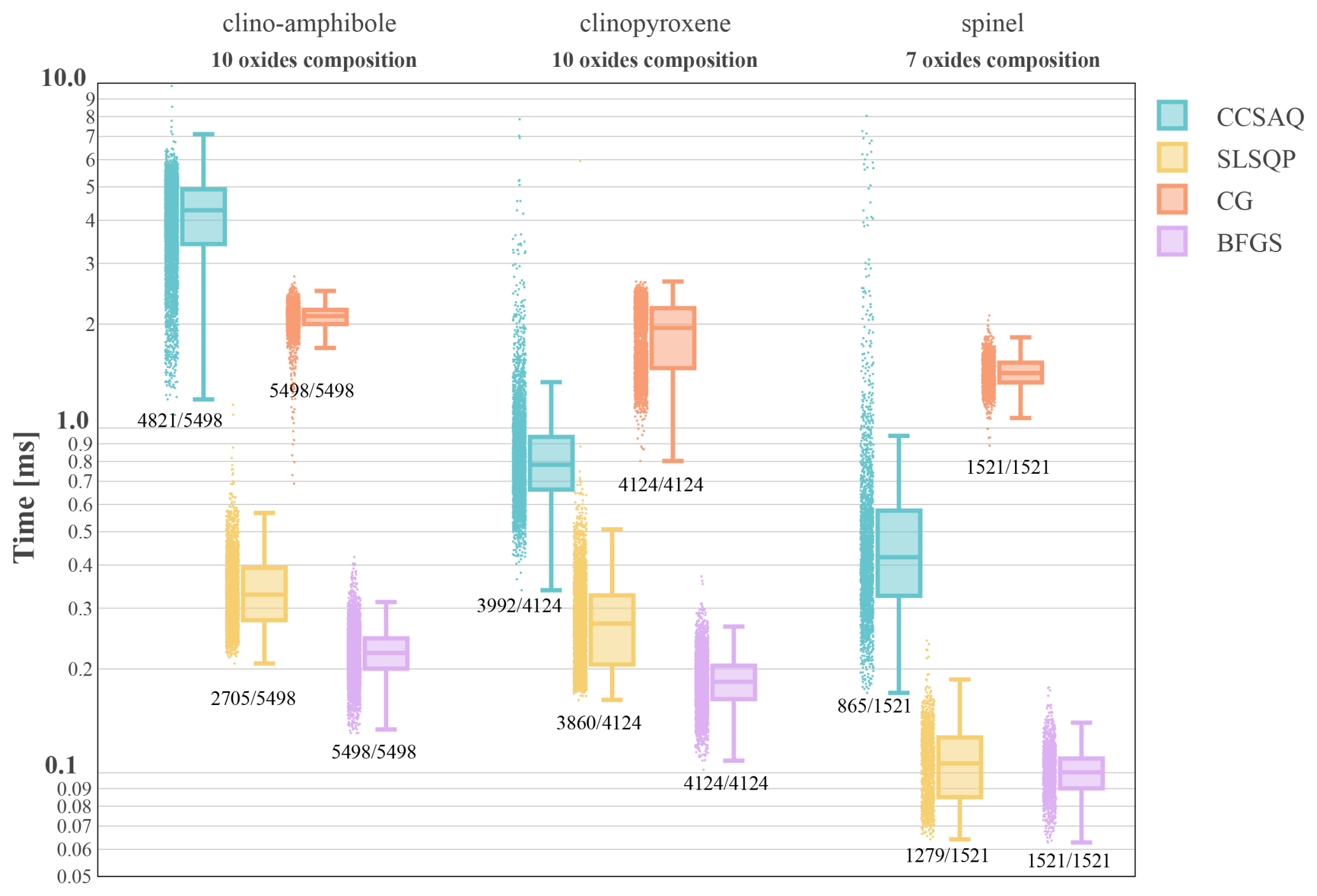
Figure 2 Minimization time box plot for tested solution phases and optimization methods. SLSQP, Sequential Least-Squares Quadratic Programming (supporting both inequality and equality constraints); CCSAQ, Conservative Convex Separable Approximation with Quadratic penalty; CG, conjugate gradiend; BFGS, Broyden-Fletcher-Goldfarb-Shanno. 5498, 4124 and 1521 starting points for clino-amphibole, clinopyroxene and spinel, respectively. Starting points were generated by evenly sampling the entire feasible space following the method presented in Riel et al. (2022). The numbers below the boxes show the number of successful minimizations over the total number of tested points.

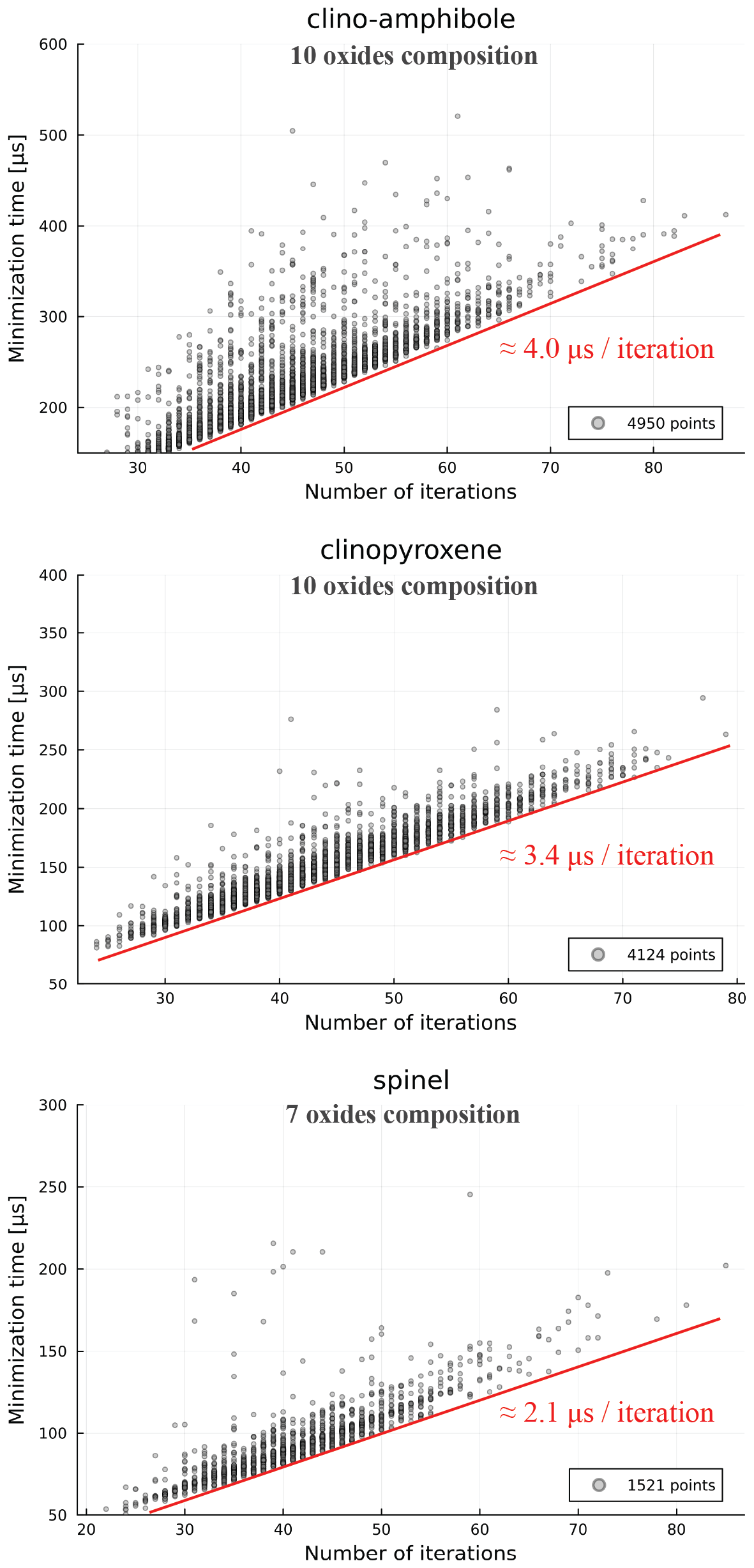
Figure 3 Number of iterations versus minimization time for the BFGS method. The red lines show the minimum minimization time per iteration.

Although the average minimization time is a good indicator of the raw performance of the algorithms, reliability of the solvers is of key importance when computing phase equilibria. In this light, we find that the bound-constrained algorithms (CG and BFGS) are far superior to the inequality constraints ones (CCSAQ and SLSQP). For instance, the bound-constrained methods (BFGS and CG) successfully minimize 100 % of the tested starting points (Fig. 2) while the inequality constraints methods show a significant amount of unsuccessful minimization reaching up to 50 % in some cases e.g., clino-amphibole minimization using SLSQP or spinel using CCSAQ (Fig. 2). The unsuccessful minimizations are related to violated inequality constraints and the inability for the algorithms (SLSQP and CCSAQ) to go back to the feasible domain.

Finally, we tested the BFGS algorithm for an equilibrium between two phases separated by a solvus i.e., an objective function containing more than one local minimum. The parameters of the test are given in Table 1 (spinel solvus) and the results are shown in Fig. 4. The bound-constrained formulation and the BFGS method perfectly captures the solvus with consistent minimization time similar to those shown in Fig. 2.

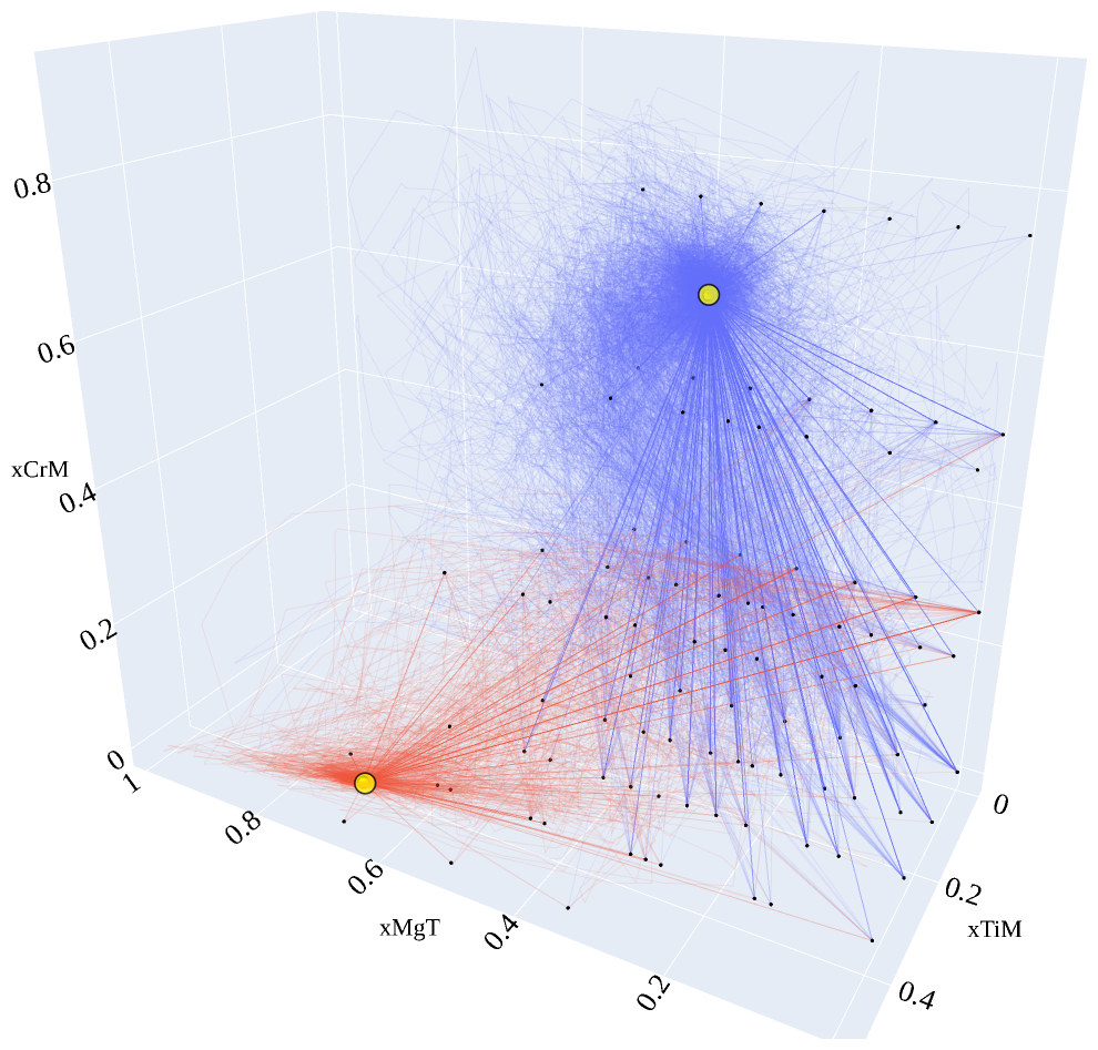
Figure 4 Minimization paths for an example of spinel solvus. The spinel solvus has been computed using the Gibbs hyperplane provided in Table 1 which was computed using MAGEMin. Black dots, starting point in the $X_{\mathrm{Cr}}^M$, $X_{\mathrm{Mg}}^T$ and $X_{\mathrm{Ti}}^M$ site fraction sub-system; yellow circles with black outline, local minimum of the solvus; red and blue lines, minimization paths from starting point to local minimum. Note that the diagram only displays a 3D sub-system of the full 10D system.

4.2 Minimization of perturbed systems

Minimization from discretized starting points allows quantification and comparison of the raw performance and stability of the algorithms (CG, BFGS and CCSAQ, see Fig. 2). However, a phase equilibrium calculation employing gradient-based methods generally involves finding a new local minimum under slightly to moderately perturbed conditions between global iterations (de Capitani and Petrakakis, 2010; Riel et al., 2022) i.e., that the distance between the starting point and the ending point during local minimization of individual phases is small. A measure of this distance can be calculated as the variation of the norm of the Gibbs hyperplane: $\Vert \mathrm{\Delta }\mathrm{\Gamma }{\Vert }_{\mathrm{2}}^{\mathrm{2}}$, where Γ is the chemical potential of the pure components of the system (oxides in our case, Table 1). In order to test the performance of the SLSQP and BFGS methods under small perturbations, we use as starting points the minima obtained by tests 1 to 3 and apply a perturbation to the Gibbs hyperplane (Table 1). The perturbation is set by applying a random rotation to the objective function which shifts the local minimum from its current position. We explore the effect of such perturbation by computing 10 000 random rotations per solution phase yielding a range of chemical potential $\Vert \mathrm{\Delta }\mathrm{\Gamma }{\Vert }_{\mathrm{2}}^{\mathrm{2}}$ varying from 0.0 to ca. 60.0. The results of the minimizations of the rotated systems are presented in Fig. 5a–c.

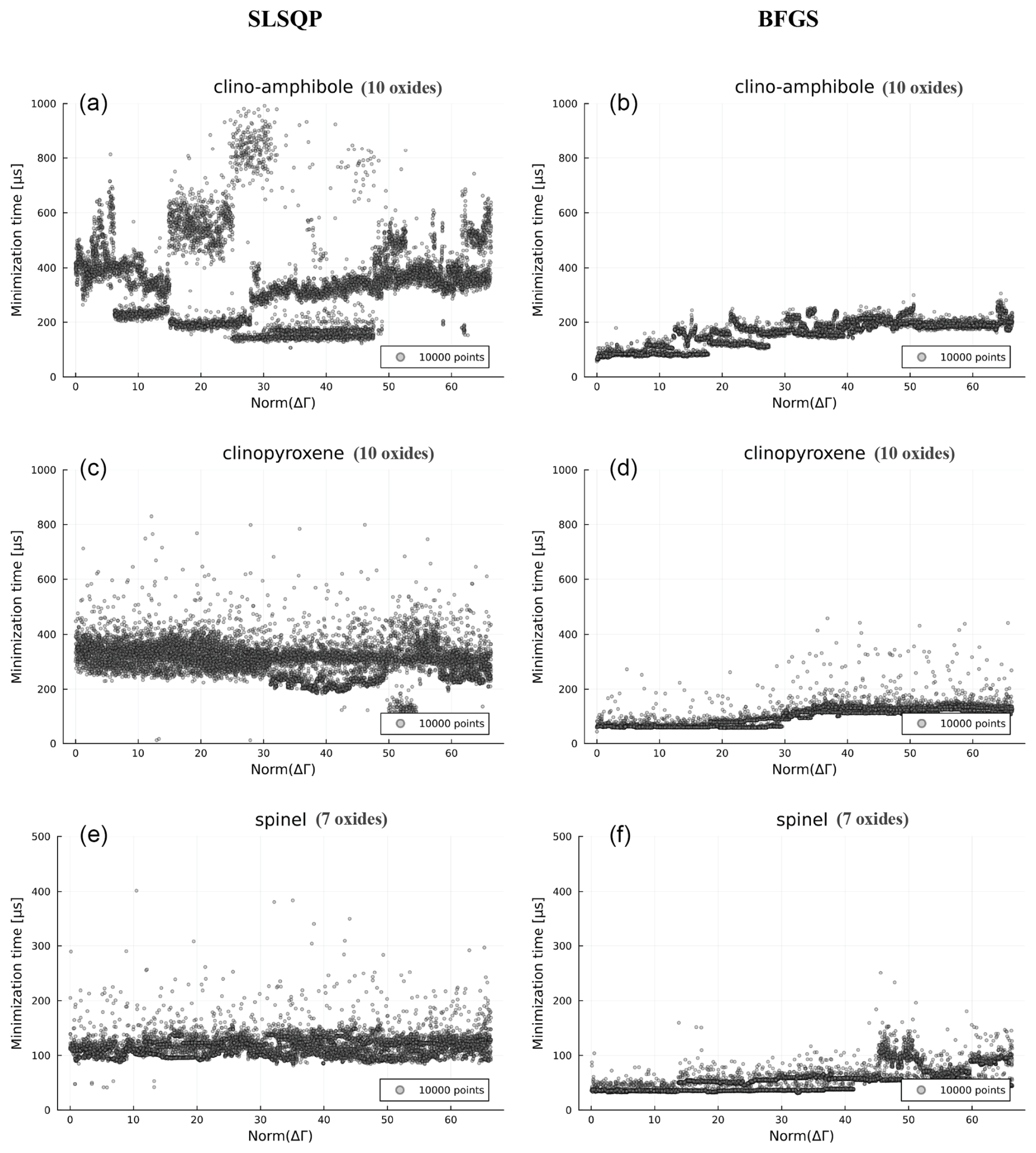
Figure 5 Minimization time for perturbed systems. (a–c) SLSQP algorithm applied to clino-amphibole, clinopyroxene and spinel, respectively. (d–f) BFGS algorithm applied to clino-amphibole, clinopyroxene and spinel, respectively. $\Vert \mathrm{\Delta }\mathrm{\Gamma }{\Vert }_{\mathrm{2}}^{\mathrm{2}}$ is a measure of the distance between the starting guess and the solution. Note that the inequality constrained SLSQP method does not show any correlation between the distance to solution and the minimization. The BFGS method, instead, exhibits a clear trend of decreasing minimization for smaller distances to solution.

For perturbed conditions, we find that the minimization time of the SLSQP algorithm does not scale with the norm of the perturbation ($\Vert \mathrm{\Delta }\mathrm{\Gamma }{\Vert }_{\mathrm{2}}^{\mathrm{2}}$) (Fig. 5a, b, c). This relationship is independent of the tested solution phase model (Fig. 5a–c). Instead, for the BFGS algorithm, the minimization time scales with the norm of the perturbation (Fig. 5d–f). For a $\Vert \mathrm{\Delta }\mathrm{\Gamma }{\Vert }_{\mathrm{2}}^{\mathrm{2}}<\mathrm{10.0}$ the minimization time is divided by a factor of ca. 2.0 to 3.0 with respect to the mean raw minimization time (Fig. 2) resulting in an average time of 70–80 µs for clino-amphibole, 50–60 µs for clinopyroxene and 30–40 µs for spinel.

We propose a revised xeos implementation using a nullspace approach, that allows using bound-constrained, rather than inequality-constrained, gradient-based optimisation methods. We tested the performance and computational reliability of different algorithms and find that the BFGS method yields the best performance, decreasing the minimization time of individual solution phases by a factor ≥10 compared to CG and CCSAQ methods and by a factor of 1.5 to 2.0 with respect to the SLSQP method (Fig. 2). Under slight perturbations, the minimization time is further decreased by a factor of 2.0 reaching down to ≤ 100 µs for clino-amphibole, ≤ 80 µs for clinopyroxene and ≤ 50 µs for spinel.

Regarding computational reliability, bound-constrained optimization methods(such as CG and BFGS), are clearly preferable over methods with inequality constraints (CCSAQ and SLSQP), which exhibit a considerable proportion of unsuccessful minimizations.

Using an bound-constrained nullspace formulation and the BFGS method, can therefore significantly improve the performance of stable phase calculations. Given that in MAGEMin, ≥ 75 % of the computational load is dedicated to local minimization of solution phase models, we estimate a general speed-up of stable phase equilibrium prediction by a factor ≥ 5. Such improvement can potentially opens up the possibility of performing 2D reactive models fluid/magma transport.