Implementation of a dry deposition module (DEPAC v3.11_ext) in a large eddy simulation code (DALES v4.4)

High-resolution data on reactive nitrogen deposition are needed to inform cost-effective policies. Large eddy simulation models coupled to a dry deposition module present a valuable tool for obtaining these high-resolution data. In this paper we describe the implementation of a dry deposition module, which is an extension of DEPAC v3.11 with co-deposition (DEPAC v3.11_ext; hereafter simply referred to as DEPAC), in a large eddy simulation code (DALES v4.4) and its first application in a real-world case study. With this coupled model, we are able to represent the turbulent surface–atmosphere exchange of passive and reactive tracers at the hectometer resolution. A land surface module was implemented to solve the surface energy budget and provide detailed information for the calculation of deposition fluxes per land use (LU) class. Both the land surface model and the dry deposition module are extensively described, as are the inputs that are needed to run them.

To show the advantages of this new modeling approach, we present a case study for the city of Eindhoven in the Netherlands, focusing on the emission, dispersion, and deposition of NO_x and NH₃. We find that DALES is able to reproduce the main features of the boundary layer development and the diurnal cycle of local meteorology well, with the exception of the evening transition. DALES calculates the dispersion and deposition of NO_x and NH₃ in great spatial detail, clearly showing the influence of local LU patterns on small-scale transport, removal efficiencies, and mixing characteristics.

1 Introduction

Eutrophication and acidification due to atmospheric deposition of reactive nitrogen have widespread impacts on biodiversity (Bobbink et al., 2010; Dise et al., 2011). Across Europe critical nitrogen loads are widely exceeded in protected nature areas, most notably in or close to source regions of ammonia and nitrogen oxides (Jonson et al., 2022). The Netherlands is a densely populated country and has a very productive agricultural sector, a combination leading to the largest emission density of reactive nitrogen compounds in Europe (EMEP/CEIP, 2023). Often, activities emitting large quantities of reactive nitrogen are located in close proximity to nature areas. For example, many farms are located within a kilometer of a nature reserve. In addition, major roads and highways may cut through or circumvent nature reserves, and some of the country's largest industrial facilities border areas declared a nature preservation area. These activities all contribute to total deposition loads on nature areas.

Deposition loads can be seen as a sum of background deposition caused by a large number of small contributions from distant sources and local deposition due to nearby sources. Traditionally, these spatial scales have been addressed by different modeling techniques applying chemistry transport models (CTMs) at the regional scale and dispersion models at the local scale. As the CTMs simulate explicit chemistry on an hour-by-hour basis on a regular grid, they assume instantaneous mixing within their grid cells and thus cannot be used to address near-source dispersion and chemistry. In contrast, local-scale modeling is often performed with Gaussian plume models driven by statistical meteorological data. These models describe hourly averaged plumes based on wind characteristics, atmospheric stability, and downwind surface roughness. Losses due to deposition and chemistry can only be taken into account through very simplified calculation rules and source depletion terms. A number of models combine a plume approach with a trajectory system with a slightly more elaborate accounting of chemical conversion, e.g., OPS (Sauter et al., 2020) and FRAME (Aleksankina et al., 2018; Singles et al., 1998). Both types of models thus have their limitations in representing processes relevant to deposition at the local scale.

The aforementioned local modeling practices prevail due to modest calculation requirements in many (regulatory) applications such as permitting practices. However, a number of applications call for the development of more detailed modeling systems for the local scale. Firstly, for reactive species the processes of turbulent dispersion, chemistry, and deposition take place on similar timescales and spatial scales and together determine the deposition patterns in a complex landscape. Atmospheric chemistry is often parameterized in these models, which leads to systematic biases in conditions that deviate from the photostationary state, especially for fast-reacting species such as NO₂ (Vilà-Guerau de Arellano et al., 1990; Grylls et al., 2019; Zhong et al., 2017). Besides the photostationary equilibrium, the NO₂ atmospheric lifetime of 2 to 12 h may cause a substantial fraction of the locally emitted NO_x to be converted into nitric acid, which deposits efficiently. Moreover, turbulent mixing timescales have been shown to impact the formation of ammonium nitrate (Aan de Brugh et al., 2013; Barbaro et al., 2015), which is supported by reports of ammonium nitrate evaporation impacting ammonia flux measurements (Zhang et al., 1995). Hence, to study the deposition of nitrogen compounds in a complex landscape in detail, a model is required that resolves the turbulent structure of the boundary layer, the chemical interactions, and the deposition processes. Secondly, modern observation systems reach temporal and spatial resolutions such that detailed modeling is required to optimize the monitoring design and interpret their results. For example, new satellite missions target resolutions of several hundred meters, scales at which plumes will be partially resolved (ESA, 2023). Recent flight campaigns already show meandering plumes from all kinds of large point sources. Fast-response instruments are being used to perform mobile measurements traversing through plumes (Twigg et al., 2022). All these observations do not fit a Gaussian plume representation as they observe an instantaneous realization of the plume at hand. To invert emission strengths from these observation systems, more detailed understanding is needed of the plume behavior and of loss terms between the source and receptor. Thirdly, the societal debate on reactive nitrogen deposition and the potential mitigation strategies, as well as the underlying science, calls for the evaluation of the highly parameterized dispersion models that are currently used in many regulatory applications.

Models that resolve turbulent flow and chemical reactions simultaneously are crucial at spatial scales of 100 m and below. Large eddy simulation (LES) models in principle have that capacity, since they resolve the atmospheric transport by the largest scales of atmospheric turbulence. They have been developed since the 1970s (Deardorff, 1970) and have been applied mostly to academic cases. In LES modeling, the turbulent flow field defined by the full Navier–Stokes equations is resolved down to certain minimum length scales and timescales. Below these scales, a sub-grid-scale (SGS) model dictates the behavior of the small-scale turbulent eddies and the dissipation of turbulent kinetic energy. In that sense, LES offers many benefits above widely applied Reynolds-averaged Navier–Stokes calculations, which only provide time-averaged properties of fluid flow (Blocken, 2015). Recent developments in computational power and coupling to large-scale models (Jansson et al., 2019; Van Stratum et al., 2019; Schalkwijk et al., 2015) have enabled the application of LES on larger spatial and temporal scales than before. Several LES codes are currently being developed towards application in air quality though the development of modules that represent, for instance, the flow around buildings (Tomas et al., 2015), gas-phase chemistry (Vilà-Guerau de Arellano et al., 2011; Kim et al., 2012; Khan et al., 2021), or anthropogenic emissions (Khan et al., 2021). These developments have significantly improved the representation of real-world cases (Maronga et al., 2020; Suter et al., 2022).

Dry deposition of gaseous and aerosol species on the (vegetated) land surface has not been explored much using LES models. Barbaro et al. (2015) studied gas–aerosol partitioning for ammonium nitrate with DALES, the Dutch Atmospheric Large Eddy Simulation model (Heus et al., 2010). They used a simplified resistance model (e.g., Wesely, 1989) including aerodynamic resistance, quasi-laminar sublayer resistance (depending on the molecular diffusivity of the gas), and bulk surface resistance for land use consisting of grass only. Clifton and Patton (2021) applied the National Center for Atmospheric Research (NCAR) LES model, coupled to a multi-layer model of the vegetation canopy with a simplified chemical mechanism. They focused on the ozone deposition to the canopy and soil, particularly on the influence of turbulence on the deposition. Subsequently, Clifton et al. (2022) extended the model with a chemical model of 41 reactions and 19 gases for ozone, NO_x(= NO + NO₂), ${\mathrm{HO}}_x(=\mathrm{•}\mathrm{OH}+{\mathrm{HO}}_{\mathrm{2}}^{\mathrm{•}})$, and isoprene chemistry. Although the dry deposition process description has also recently been included in the PALM LES code (Khan et al., 2021), there has not been specific attention to its application.

Our overall goal is to study the process affecting nitrogen deposition at the landscape scale using the DALES system. In this work, we coupled a dry deposition module to the LES code, with the goal of enabling the representation of dry deposition of trace gases over a realistic land use mosaic. Our approach focuses on the application of the well-established dry deposition parameterization DEPAC (Deposition of Acidifying Compounds; Van Zanten et al., 2010) in DALES. To demonstrate the capability of the model to simulate tracer dispersion and dry deposition, we set up a case study over the city of Eindhoven, which is the fourth largest city in the Netherlands. In contrast to other large cities in the Netherlands, its inland location ensures that we can use the meteorological forcing as applied here, since there are no coastlines or large water bodies in the domain that could induce secondary circulations. The city is surrounded by major highways and an airport and is embedded in an area with intensive animal husbandry. Hence, it is one of the regions where reactive nitrogen emissions are greatest and result in exceedance of the critical loads in the nature areas adjacent to the city. In our current analysis, we focus on the dispersion and dry deposition of two passive tracers (NO_x and NH₃) and their dependence on atmospheric and LU properties. Chemical conversions are not yet included in this study.

This paper is organized as follows: in Sect. 2, we describe the DALES model and the DEPAC dry deposition module, as well as the implementation of DEPAC in DALES. Next, we demonstrate the application of the system in a case study for Eindhoven (Sect. 3). This case study is a first demonstration of dry deposition at high resolution in a complex landscape. Therefore, we will focus on the qualitative aspects and highlight directions for future development. A first evaluation against NH₃ concentration and flux observations at Cabauw is included in Sect. 4. Finally, in Sect. 5, we summarize our conclusions.

2 Model description

2.1 DALES

The Dutch Atmospheric Large Eddy Simulation (DALES) is rooted in the LES code of Nieuwstadt and Brost (1986) and Cuijpers and Duynkerke (1993). The model resolves turbulent transport processes based on the filtered Navier–Stokes equations combined with the Boussinesq approximation. DALES uses 1.5-order closure to parameterize subfilter-scale processes. A complete description of DALES v3.2 is given by Heus et al. (2010). Since version 3.2, a few additions have been made, including improved restart possibilities, new advection schemes, an improved radiation model, and optimized sub-grid calculations.

DALES has been applied in studies on the transport and chemical conversion of reactive species in the boundary layer. Vinuesa and Vilà-Guerau de Arellano (2003) studied the effect of turbulence on reactive tracer transport, and Vilà-Guerau de Arellano et al. (2005) studied the influence of cumulus clouds on the transport of reactive tracers. In a series of case studies over tropical forests, Vilà-Guerau de Arellano et al. (2009) used DALES to study the diurnal cycle of isoprene emissions, Vilà-Guerau de Arellano et al. (2011) performed case studies on the diurnal cycle of concentrations of reactive species, and Ouwersloot et al. (2011) studied the influence of turbulence on the reactivity of chemical species. These studies did not take dry deposition of trace gases into account.

In an idealized DALES experiment, Aan de Brugh et al. (2013) studied the gas–particle partitioning of ammonium nitrate in the convective boundary layer (CBL) at midlatitudes. They suggest that turbulent mixing in the CBL causes horizontal and temporal variability in aerosol nitrate mixing ratios, which leads to an apparent downward flux of ammonium nitrate that might be interpreted as nitrate deposition. Barbaro et al. (2015) expanded that case study by including the surface exchange of ammonium nitrate and related gas-phase species in a simplified way. Recently, Schulte et al. (2022) studied the turbulent dispersion of NH₃ with DALES, with the goal of assessing the representativity of NH₃ observations. In their simulations, they prescribed a constant deposition flux for NH₃ based on annual average observations.

2.2 Land surface module

The land surface and the atmosphere above it form a tightly coupled system on diurnal (and longer) timescales (Betts, 2004; Van Heerwaarden et al., 2010). The direction and strength of the exchange of heat, moisture, and momentum are driven by this coupling. Moreover, land use plays an important role in dry deposition because the properties of the land surface regulate the uptake of pollutants. Therefore, the relationship between deposition fluxes of reactive compounds, the (vegetated) land surface, and heat and moisture fluxes is integral to our approach of coupling a deposition module to DALES.

The state of the vegetation, the soil, and their exchanges of heat and water with the atmosphere in DALES are described by a land surface model (LSM) that is based on the Tiled ECMWF Scheme for Surface Exchanges over Land with revised hydrology (HTESSEL) land surface scheme (ECMWF, 2021; Balsamo et al., 2009). In HTESSEL, sub-grid surface types are represented by tiles. Each tile represents an LU type for which an energy balance equation is solved. This results in a sensible (H) and latent (LE) heat flux per tile, which is then aggregated to a grid cell. Soil moisture content and soil temperature are calculated in a four-layer soil model. Precipitation and dew fall are collected in an interception layer. Canopy conductance can be calculated in two different ways in HTESSEL: following the Jarvis–Stewart approach or following a plant-physiology-based approach (A-gs). Here, we followed the former approach. Monin–Obukhov similarity theory (MOST) is used to estimate the resistances associated with transport between the lowest model level and the land surface.

We made modifications in the LSM to enable the coupling with the deposition module. Most importantly, we made the number and types of land use classes available flexible. In that way, the land use (LU) types relevant for dry deposition can be selected flexibly, and relevant properties can be assigned. Here, we aligned the LU types with those available in DEPAC (see Table B1).

2.3 The DEPAC deposition module

2.3.1 Description of the deposition module

To account for dry deposition in local air quality models, one of two approaches is generally followed. The first and simplest approach is the assumption of a constant deposition velocity that is tabulated for each species. This approach has three important downsides. First, there is a significant influence of the wind speed and the turbulence generated near the surface on the transport of species to the surface which is not covered when assuming constant deposition velocity. It is therefore important to incorporate the surface roughness and the surface type in the calculation of dry deposition of both gaseous and aerosol species. Second, variations in plant physiology, temperature, relative humidity, and radiation play an important role in determining the dry deposition velocity (see, for instance, Emberson et al., 2000b), whereas a constant deposition velocity only contains static influences. Third, the concept of a constant deposition velocity is also inappropriate since it assumes a constant deposition velocity with height near the surface, which does not hold for chemically reactive species like NO_x (Vinuesa and Vilà-Guerau de Arellano, 2003). Including these parameters in the parameterization of dry deposition is essential to get insight into diurnal and seasonal cycles as well as the effect of meteorology on deposition and to get a realistic representation of atmospheric concentrations and deposition.

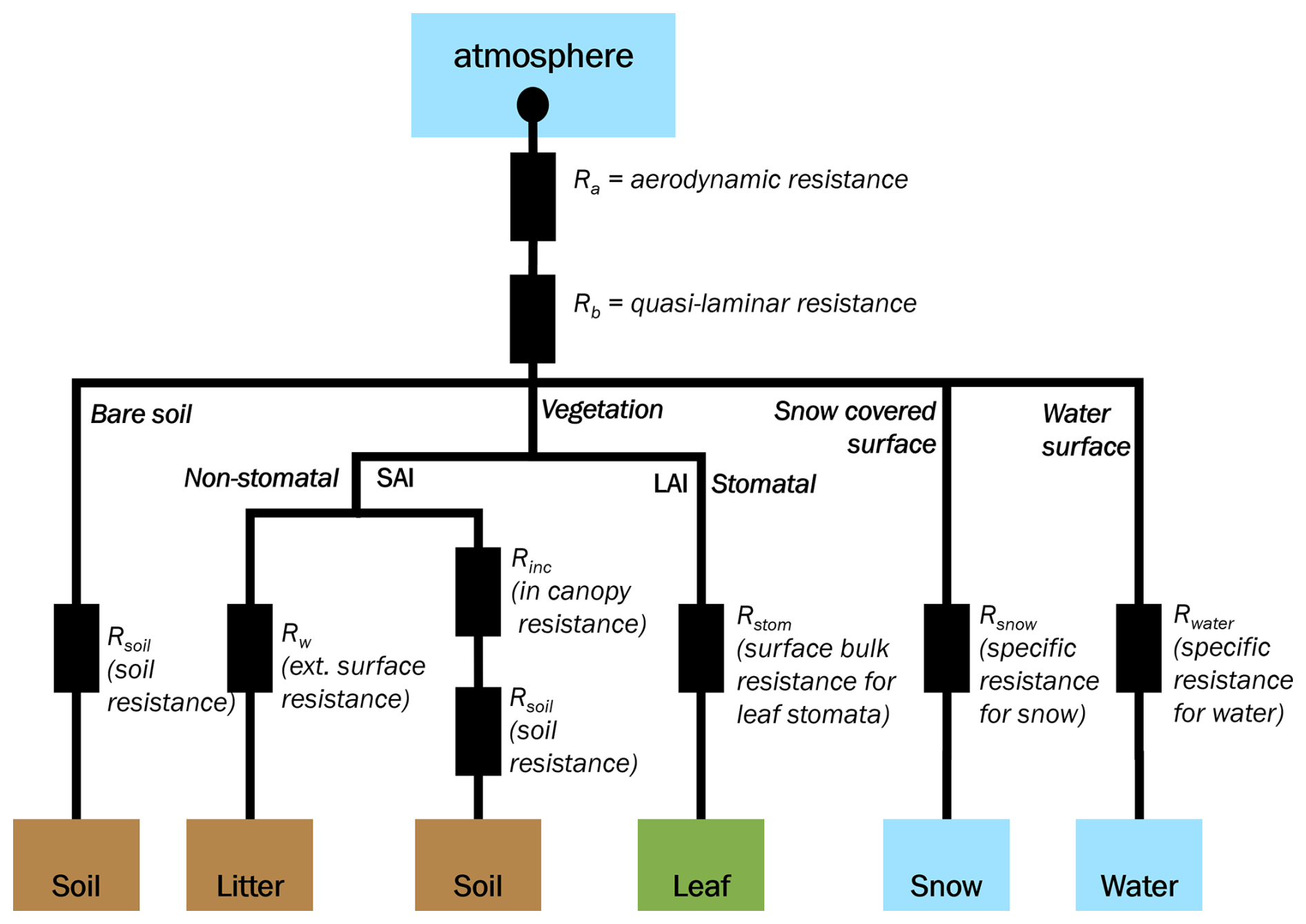
The second and most widely used approach is the resistance model attributed to Wesely (1989), who modeled the deposition velocity V_d (m s⁻¹) as the reciprocal sum of three resistances: the aerodynamic resistance R_a (s m⁻¹), the quasi-laminar sublayer resistance R_b (s m⁻¹), and the canopy resistance R_c (s m⁻¹).

$$\begin{array}{}\text{(1)}& V_{\mathrm{d}}={\displaystyle \frac{\mathrm{1}}{R_{\mathrm{a}}+R_{\mathrm{b}}+R_{\mathrm{c}}}}\end{array}$$

The DEPAC deposition module applied in this work is an implementation of the resistance model. A schematic representation of the model is shown in Fig. 1, with its deposition pathways to vegetated and non-vegetated surfaces, each with their own specific parameters. It offers a fine-grained differentiation of deposition on nine different land use classes.

Figure 1 Schematic representation of the dry deposition model in DALES.

The DEPAC module is a well-established module for dry deposition calculations. It is used as a dry deposition module in the air quality models LOTOS-EUROS (Manders et al., 2017, 2022) and OPS (Sauter et al., 2020). A theoretical analysis of the sensitivity of DEPAC to several of its input parameters is given by Van Zanten et al. (2010). Further, it has been evaluated against observed deposition fluxes over forests (Melman et al., 2025; Wintjen et al., 2022) and dune ecosystems (Jongenelen et al., 2025; Vendel et al., 2023). These analyses have shown that the parameterizations of compensation point and the external resistance (R_w) contribute most to uncertainties in calculated deposition (and emission) fluxes of NH₃.

2.3.2 Calculation of resistances

The calculation of the aerodynamic resistance R_a is based on the meteorological conditions and the surface roughness z₀ (m). R_a is common to all species and determined from the stability of the atmosphere and the surface roughness. Because the surface roughness depends on the land use type, in DALES we calculate the R_a per land use type in a grid cell.

$$\begin{array}{}\text{(2)}& R_{\mathrm{a}}={\displaystyle \frac{\mathrm{1}}{u^{*}\cdot {\mathrm{\Phi }}_h}},\end{array}$$

where u^* is the friction velocity (m s⁻¹) and Φ_h is a dimensionless parameter that depends on atmospheric stability and is calculated from MOST (Businger et al., 1971).

The quasi-laminar resistance R_b is determined from the friction velocity and the molecular diffusivity of the species in the air.

$$\begin{array}{}\text{(3)}& R_{\mathrm{b}}={\displaystyle \frac{\mathrm{2}}{\mathit{\kappa }\cdot u^{*}}}\cdot {\left({\displaystyle \frac{Sc}{Pr}}\right)}^{(\mathrm{2}/\mathrm{3})},\end{array}$$

in which κ is the von Kármán constant (–), Sc is the dimensionless Schmidt number (–), defined as the ratio between the kinematic viscosity of the air and the mass diffusivity of the species in the air, and Pr is the dimensionless Prandtl number (–), defined as the ratio between the kinematic viscosity of the air and the heat diffusivity of the air (definition according to Wesely and Hicks, 1977). Although there is a species dependence (in $Sc/Pr$) in R_b, it usually plays a minor role because the quasi-laminar layer is usually very thin (of the order of $\mathit{\nu }/u^{*}$, where ν is the kinematic viscosity of air) and R_b is therefore small. In the calculation of R_b, the molecular diffusivity and viscosity are used.

The canopy resistance R_c is the result of three parallel resistances: the stomatal resistance, the soil resistance, and the external surface resistance. The canopy resistance R_c is calculated from stomatal and non-stomatal conductances and resistances based on the model of Erisman et al. (1994).

$$\begin{array}{}\text{(4)}& R_{\mathrm{c}}={\left({\displaystyle \frac{\mathrm{1}}{R_{\mathrm{stom}}}}+{\displaystyle \frac{\mathrm{1}}{R_{\mathrm{soil},\mathrm{eff}}}}+{\displaystyle \frac{\mathrm{1}}{R_{\mathrm{w}}}}\right)}^{-\mathrm{1}}\end{array}$$

Non-stomatal transport is divided into transport to external surfaces (cuticles and other surfaces, represented by resistance R_w in s m⁻¹) and transport through the canopy to the soil ($R_{\mathrm{soil},\mathrm{eff}}=R_{\mathrm{inc}}+R_{\mathrm{soil}}$ in s m⁻¹). For the latter, a distinction is made between snow-covered and open soil. The stomatal resistance R_stom (s m⁻¹) is implemented according to Emberson et al. (2001). The stomatal conductance is controlled by the type of vegetation, its phenological state, temperature, relative humidity, insolation, and the potential for water of the soil.

In general, there are two main variants of this resistance approach. The first assumes a concentration of species on the deposition surface of zero; the deposition flux F_dep ($\mathrm{\mu }\mathrm{g}{\mathrm{m}}^{-\mathrm{2}}{\mathrm{s}}^{-\mathrm{1}}$) is then modeled as the product of the deposition velocity and the concentration in the atmosphere χ_atm (µg m⁻³) (e.g., Simpson et al., 2012). Although it performs well for compounds that are completely absorbed through the surface, this approach induces possible overestimation of the deposition fluxes and does not anticipate re-emission of species from the surface into the atmosphere. Especially for NH₃ during growing seasons, this can result in unrealistic deposition fluxes (Wichink Kruit et al., 2007).

The second variant of the resistance approach considers a nonzero concentration on the deposition surface, called a compensation point χ_comp (µg m⁻³). This is the concentration that is in equilibrium with the reservoir of the species, in this case ammonium, under the surface. When ammonia concentrations in the atmosphere are higher than the compensation point, deposition occurs. Emission occurs when the atmospheric ammonia concentration is below the compensation point. Hence, the exchange is bidirectional. The resulting flux is calculated with

$$\begin{array}{}\text{(5)}& F_{\mathrm{dep}}=-V_{\mathrm{d}}\cdot \left({\mathit{\chi }}_{\mathrm{atm}}-{\mathit{\chi }}_{\mathrm{comp}}\right).\end{array}$$

The compensation point is defined for the stomatal and external surface deposition routes, and its parameterization is given in Sect. 2.3.3.

Currently, the deposition model uses a dedicated land surface model that is different from HTESSEL. While HTESSEL is used for the calculation of energy and moisture fluxes, the land surface model in the deposition model is dedicated to the deposition flux calculations. Future development plans include the integration of these two modules, but they are currently used in parallel. In dry conditions, this is not a problem, but there is a caveat to this approach regarding wet surfaces. HTESSEL defines a dedicated land surface class for wet surfaces, regardless the underlying land surface. The land surface model for deposition uses a flag for each land surface type that signals whether it is dry or not. Due to these different implementations, cases with wet soil and/or canopy cannot be simulated properly, as the current implementation of the deposition model ignores the fact that the soil/canopy is wet (it assumes dry conditions). In our case study, we circumvented this problem, since the Royal Dutch Meteorological Institute (KNMI) weather data at the location of Eindhoven airport showed that the date of our simulations was preceded by a prolonged period of dry conditions (11 d without any precipitation).

2.3.3 Canopy exchange

The first term on the right in Eq. (4), the deposition resistance for stomatal exchange, is defined in Eq. (6) below. Per LU class, a maximum canopy conductivity $G_{\mathrm{s}}^{max}$ (m s⁻¹) is defined, which signifies the conductivity in the case of fully opened leaf stomata. The stomata may not to be fully open for a number of reasons; for each of these, a dimensionless parameter between zero and 1 is multiplied with $G_{\mathrm{s}}^{max}$ to scale the transport. f_phen is the correction factor for plant phenology, f_swp corrects for the soil water potential, f_vpd is a correction for the vapor pressure deficit, f_T is a temperature correction, and f_PAR is the correction for photoactive radiation (Emberson et al., 2000b, a).

$$\begin{array}{}\text{(6)}& R_{\mathrm{stom}}={\left(G_{\mathrm{s}}^{max}\cdot f_{\mathrm{phen}}\cdot f_{\mathrm{swp}}\cdot f_{\mathrm{vpd}}\cdot f_{\mathrm{T}}\cdot f_{\mathrm{PAR}}\right)}^{-\mathrm{1}},\end{array}$$

where the correction factor for phenology f_phen and the correction factor for soil water potential f_swp are both assumed to be equal to 1.0. This assumption is justified as follows: for the current LU classes, the impact of phenology is minimal (Van Zanten et al., 2010). Instead, the seasonal variation in vegetation phenology is accounted for by using a leaf area index (LAI in ${\mathrm{m}}_{\mathrm{leaf}}^{\mathrm{2}}{\mathrm{m}}_{\mathrm{ground}\mathrm{surface}}^{-\mathrm{2}}$) that changes according to the vegetation's growing season.

$$\begin{array}{}\text{(7)}& G_{\mathrm{s}}^{max}=g_{\mathrm{s}}^{max}\cdot \mathrm{LAI},\end{array}$$

where $g_{\mathrm{s}}^{max}$ is the maximum leaf conductance (m s⁻¹). Similarly, the influence of soil water potential in northwestern Europe is expected to be limited (Van Zanten et al., 2010).

Specifically for NH₃, the stomatal compensation point χ_s (µg m⁻³) is calculated from an equilibrium correlation (Wichink Kruit et al., 2007). Γ_s is the dimensionless ratio between the apoplastic molar ${\mathrm{NH}}_{\mathrm{4}}^{+}$ and H⁺ concentrations given by (Wichink Kruit et al., 2010),

$$\begin{array}{}\text{(8)}& {\displaystyle }{\mathit{\chi }}_{\mathrm{s}}={\displaystyle \frac{\mathrm{2.75}\times {\mathrm{10}}^{\mathrm{15}}}{T_{\mathrm{s}}+\mathrm{273.15}}}\exp \left({\displaystyle \frac{-\mathrm{1.04}\times {\mathrm{10}}^{\mathrm{4}}}{T_{\mathrm{s}}+\mathrm{273.15}}}\right)\cdot {\mathrm{\Gamma }}_{\mathrm{s}}\left(T_{\mathrm{s}}\right)\text{(9)}& {\displaystyle }{\mathrm{\Gamma }}_{\mathrm{s}}\left(T_{\mathrm{s}}\right)=\mathrm{362}\cdot {\mathit{\chi }}_{\text{a,4\hspace{0.17em}m,long term}}\cdot \mathrm{4.7}\cdot \exp (-\mathrm{0.071}{T}_{\mathrm{s}})\end{array}$$

in which χ_{a,4 m,long term} is the “long-term” mean concentration of NH₃ at 4 m above the ground (µg m⁻³) and T_s is the leaf surface temperature (°C). In our application, we apply a monthly mean concentration for χ_{a,4 m,long term}. This approach was chosen because it is unknown how much of the depositing species accumulates in the vegetation; there is no mass balance of the vegetation. Instead, the compensation point is estimated by assuming that the accumulated amount of a species in the vegetation is in equilibrium with its long-term mean atmospheric concentration.

External leaf surface exchange is covered by the resistance R_w, as defined in Eq. (10), with RH being the relative humidity (%), and $\mathit{\alpha }=\mathrm{2}\mathrm{s}{\mathrm{m}}^{-\mathrm{1}}$ and β=12 are empirical model parameters (Sutton and Fowler, 1993). The deposition model uses an additional correction factor dependent on the surface area index (SAI in ${\mathrm{m}}_{\mathrm{deposition}\mathrm{surface}}^{\mathrm{2}}{\mathrm{m}}_{\mathrm{ground}\mathrm{surface}}^{-\mathrm{2}}$) to account for differences between SAI of the local vegetation type and the SAI at the measuring site where the compensation point χ_w was determined (Haarweg, Wageningen, The Netherlands). T_w is the surface temperature ( °C) and Γ_w is the dimensionless molar ratio between the ${\mathrm{NH}}_{\mathrm{4}}^{+}$ and H⁺ concentrations in the external leaf surface water (Van Zanten et al., 2010; Wichink Kruit et al., 2010).

$$\begin{array}{}\text{(10)}& R_{\mathrm{w}}={\displaystyle \frac{{\mathrm{SAI}}_{\mathrm{Haarweg}}}{\mathrm{SAI}}}\cdot \mathit{\alpha }\exp \left({\displaystyle \frac{\mathrm{100}-\mathrm{RH}}{\mathit{\beta }}}\right)\end{array}$$

For freezing conditions, a fixed value of R_w=200 s m⁻¹ is assumed.

A compensation point can be calculated for the external surfaces in analog to Eq. (8) by substituting Γ_w for Γ_s. Specifically for NH₃ over grassland, Γ_w is defined according to the empirical relation in Eq. (11), in which χ_a,4 m is the compensation point at 4 m (Wichink Kruit et al., 2010). For external surfaces, it is assumed that there is always a thermodynamic equilibrium between the surface and its surroundings. Therefore, χ_a,4 m has the same value as the atmospheric concentration.

$$\begin{array}{}\text{(11)}& {\mathrm{\Gamma }}_{\mathrm{w}}\left(T_{\mathrm{w}}\right)=\mathrm{1.84}\times {\mathrm{10}}^{\mathrm{3}}\cdot {\mathit{\chi }}_{\mathrm{a},\mathrm{4}\mathrm{m}}\cdot \exp (-\mathrm{0.11}{T}_{\mathrm{w}})-\mathrm{850}\end{array}$$

2.3.4 Soil exchange

Depositing species first have to travel through the canopy before they reach the soil. The effective soil resistance is therefore calculated as the sum of the in-canopy resistance R_inc and the soil resistance R_soil.

$$\begin{array}{}\text{(12)}& R_{\mathrm{soil},\mathrm{eff}}=R_{\mathrm{inc}}+R_{\mathrm{soil}}\end{array}$$

The in-canopy resistance is a function of LU type, the height of the vegetation h (m), the SAI, and the friction velocity u^* (Van Pul et al., 2008):

$$\begin{array}{}\text{(13)}& \begin{array}{rl}& R_{\mathrm{inc}}=\\ & \left\{\begin{array}{ll}\frac{b\cdot h\cdot \mathrm{SAI}}{u^{*}}& u^{*}>\mathrm{0},\text{arable land, permanent crops, forest}\\ \mathrm{1000}\mathrm{s}{\mathrm{m}}^{-\mathrm{1}}& u^{*}=\mathrm{0},\text{arable land, permanent crops, forest}\\ \mathrm{0}\mathrm{s}{\mathrm{m}}^{-\mathrm{1}}& \text{water, urban, desert}\\ \mathrm{\infty }\mathrm{s}{\mathrm{m}}^{-\mathrm{1}}& \text{grass, other},\end{array}\right.\end{array}\end{array}$$

in which b is an empirical constant (14 m⁻¹).

The SAI depends on the LAI and the LU type. Some LU classes have no SAI (SAI=0 for water, barren land, and urban), some have a constant value (SAI=b_SAI for arable land, grassland, and semi-natural land), and for others it depends on the LAI ($\mathrm{SAI}=a_{\mathrm{SAI}}\cdot \mathrm{LAI}+b_{\mathrm{SAI}}$ for permanent crops and forests). In the case that one of the resistances is irrelevant (e.g., in the case of stomatal resistance for aqueous surfaces), the resistance value is set to −9999, which is a special value to indicate that the resistance is not to be considered in the calculation of the deposition velocity.

The parameters of the in-canopy resistance are defined for nine different LU classes (see Table A2). The LAI is a function of the time of year and the growing season per LU class (see Van Zanten et al., 2010).

The soil resistance is species-dependent and, to a lesser extent, LU-dependent (except for frozen, wet, and snow-covered soil). For NH₃, NO₂, and NO, the values are presented in Table A3. These values are based on Erisman et al. (1994) but adapted to the values used in the DEPAC v3.11 implementation in LOTOS-EUROS v2.2 (Manders et al., 2022). Finally, the compensation point of the soil can be calculated similarly to the stomata (Eq. 8), with Γ_soil substituted for Γ_s, the value of which is also given in Table A2.

2.3.5 Implementation in DALES

In the main driver of DALES, for each time step (i.e., every few seconds), the dry deposition routine is called in a section of surface routines after the radiation terms are calculated and before advection and diffusion terms are calculated. First, the necessary parameters like LAI and SAI are calculated based on values from a parameter table. Then the deposition budget is calculated for each depositing tracer by a call to the DryDepos_Gas routine in the dry deposition module. Finally, in a loop over all depositing tracers the deposition budget for each tracer is added to the tracer tendency array in all surface cells.

2.4 Initial and boundary conditions

The bottom boundary condition for DALES is formed by the soil and LU properties. Representation of LU properties is especially important for dry deposition calculations. We use the TOP10NL LU map at 10×10 m² (PDOK, 2023) that is translated to the land surface types originally defined in DEPAC according to Table B1. Soil type follows the BOFEK soil map Heinen et al. (2022) and soil hydraulic properties (Van Genuchten, 1980).

For meteorological variables, we apply doubly periodic boundary conditions, which means that forcings are horizontally homogeneous but vary in time and height (Van Stratum et al., 2023). In this approach, the initial conditions (atmosphere and soil) and a number of time- and height-varying large-scale processes acting as forcings on the LES domain are derived from routine meteorological variables. These forcings, both as state variables like temperature, humidity, or wind and as tendencies of a state variable, are then added to the prognostic LES equations. The surface energy balance calculation is very sensitive to soil moisture and therefore needs to be initialized at a realistic value. The open-source Python package “Large-eddy simulation and Single-column model – Large-Scale Dynamics” or (LS)²D (Van Stratum et al., 2023) was used to create initial and boundary layer profiles as input for DALES (sources available from https://github.com/LS2D/LS2D, last access: 20 October 2023) from ERA5 reanalysis data (Hersbach et al., 2020).

2.5 Anthropogenic emissions

For realistic simulation of passive and reactive tracers at resolutions of tens of meters, detailed information is needed about their emissions at this scale. The emissions of NO_x and NH₃ we use are based on the official gridded emissions for the Netherlands (the Dutch Emission Registration, ER) for 2018 (RIVM, 2018). The official data contain emissions from more than 700 source types, which are aggregated into 15 sectors. Each source type gets assigned a spatial fraction map that is used to downscale the emissions. This fraction map describes the fraction of the emissions in each 1×1 km² grid cell of the inventory that is assigned to the 50×50 m² grid cells of DALES. Hourly emission fluxes are calculated from annual emission totals using fixed monthly, daily, and hourly time profiles. This spatial and temporal interpolation, however, creates a large uncertainty in the emission dataset, which will cause uncertainty in the timing and magnitude of emission peaks on a given day and therefore in the calculation of concentrations.

For the industry, households, and commercial activities the Basisregistratie Adressen en Gebouwen (BAG) is used (Kadaster, 2024). The BAG contains information on locations of buildings, number of addresses in each building, their size, and their function, which we use to link each building to one of these three categories. The number of addresses is used to calculate the fractions. A national database of the road network (Nationaal Wegenbestand, 2021 (NWB, 2024) was used to make fraction maps for road transport on different road types (highways, main roads, and residential roads) based on the total road length within each grid cell. For agricultural activities, fractions maps were made for livestock, arable land, and general agricultural activities based on the Basisregistratie Gewaspercelen (BRP) dataset with information on locations of agricultural plots and crop types (NGR, 2024). For railroads a map of railroad tracks is used (Prorail, 2020), and for inland shipping we use inland waterways from the same database as the road network (NWB, 2024). Finally, we use a population density map at 100 m resolution for several other source types (CBS, 2023). This resulted in a total of 12 fraction maps.

For the major point sources (mainly industrial), exact locations and emission heights are provided. For non-point sources the emission height is at ground level. For the DALES setup in this work, ground level means the height of the lowest vertical level, which is between 0 and 20 m. Plume rise has not yet been implemented in DALES. The effect of this is limited in this study since there are only a few stacks in the current domain. In the current approach, emissions on city roads appear much less intense than on highways (by a factor of approximately 50). This is caused by the way emissions are estimated and downscaled in our current emissions preprocessor. It is still under development; work is being done on the development of a more dynamic emission model, which does not imply fixed time profiles but takes seasonal, meteorological, and environmental factors into consideration. For example, the spatiotemporal variability of ammonia emissions is strongly dependent on agricultural practices, livestock distribution, crop distribution, and meteorology (Ge et al., 2023).

3 Eindhoven case study

To demonstrate the ability of DALES coupled to a dry deposition scheme to represent nitrogen transport and deposition at high spatial resolution, we performed simulations for a full diurnal cycle over a domain around the city of Eindhoven (Fig. 2). We chose a day with clear-sky convective conditions (16 June 2022). The month of June in 2022 was warm with a lot of sunshine but also a lot of rainfall in the Netherlands. The day of our case study fell in a sunny and dry weather period that started on 9 June. The wind direction during this period was mostly from the northeast, bringing warm and dry air masses. On the day after our case study (17 June), temperatures increased to tropical values (above 30 °C). The size of the model domain is 22×16 km², and it is divided into 440×320 grid cells of 50×50 m² each. In the vertical direction, the domain extends up to 8.5 km and is divided into 176 levels. Near the surface, the level thickness Δz is 20 m, and it gradually increases to 95 m at the top of the domain according to the equation $\mathrm{\Delta }z=\mathrm{\Delta }{z}_{\mathrm{0}}\cdot (\mathrm{1}+\mathrm{0.009}{)}^{iz}$ , where Δz₀ is the depth of the bottom layer and iz the index of the vertical grid.

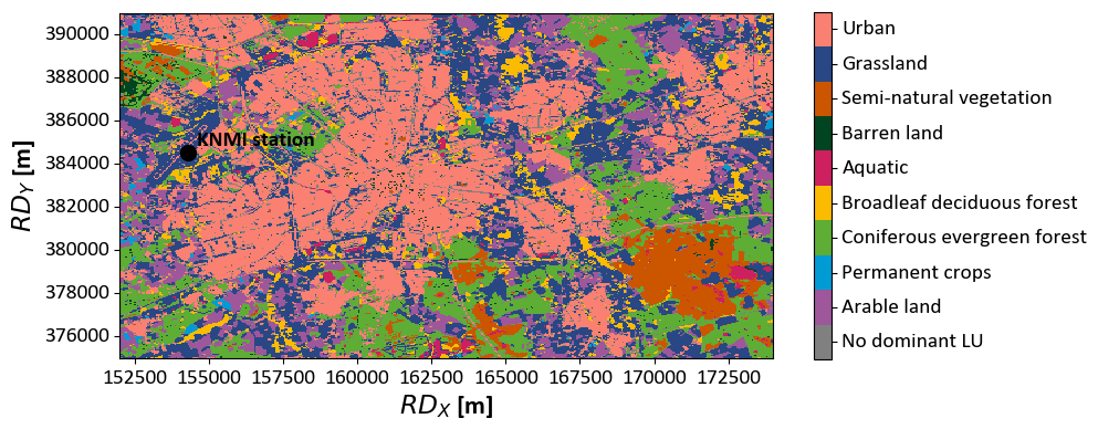
Figure 2 Map of the Eindhoven domain showing the land use and the locations of the KNMI measurement station (black dot). The map is plotted using Rijksdriehoeks (RD) coordinates (EPSG 28992).

Hourly observations of standard meteorological variables were available from the KNMI weather station at Eindhoven airport (KNMI, 2024b), station no. 370). The weather data at the location of Eindhoven airport showed that the date of our simulations was preceded by a prolonged period of dry conditions (11 d without any precipitation). Therefore, it was justified to use the equations for dry land in the model. Attenuated backscatter profiles from the CHM15k ceilometer at Maastricht Aachen airport were retrieved from KNMI (KNMI, 2024a). They provide daily aggregated files at five sites in the Netherlands, Maastricht Aachen airport being the closest to Eindhoven.

The profiles of NO_x and NH₃ concentrations were initialized to typical values in a shallow boundary layer, since the calculations start at night. NO_x was set to 1.0 ppb from the surface up to 200 m and 0.5 ppb up to 1250 m high to simulate the residual layer of the previous day. For NH₃, there is only the 200 m boundary layer with a concentration of 2.7 ppb. The concentration values are typical background concentrations measured in and around Eindhoven. Finally, it is important to note that the present calculations do not include atmospheric chemistry yet, so only emission, transport, and deposition are calculated.

3.1 Diurnal cycle, vertical mixing

Calculated sensible heat flux (H) and latent heat flux (LE) data from the DALES simulation were compared to the original ERA5 data that were used as forcing (see Fig. 3). The sensible heat flux becomes positive around 07:00 local time and peaks around 14:00 LT. Overall, the simulations match ERA5 data well, except for the hours around midday, when the sensible heat flux is larger by about 100 W m⁻² in DALES, and the latent heat flux is smaller by about 50 W m⁻². A possible explanation is the difference in local LU properties in DALES compared to the ERA5 dataset. DALES in the current setup includes nine LU types (Sect. 2.4), whereas the ECMWF IFS only includes five. Moreover, the resolution of the TOP10NL map in DALES is much higher than the LU map from ECMWF IFS (10 m versus 1 km), so the local landscape is represented in more detail. This leads to differences in the radiative properties of the surface, which will affect the amount of soil moisture and the surface energy balance.

The virtual potential temperature (θ_v), specific humidity (q_t), and wind speed (U) and direction (WDIR) are presented in Fig. 4, together with reanalysis data from the ERA5 dataset. ERA5 data are available at a 0.25° × 0.25° resolution, corresponding to a 28 × 17 km² area around Eindhoven, compared to the present domain-averaged DALES results on an area of 22 × 16 km². Downscaling of the meteorological quantities from ERA5 is handled well by DALES, since all quantities follow the ERA5 data closely, though the wind speed is slightly underestimated.

Local observations from a weather station at Eindhoven airport are also plotted in the figure. Since the wind speed is rounded to the nearest integer value and the wind direction is rounded to the nearest full degree, the precisions of the measurements are at least 0.29 m s⁻¹ and 3°, respectively. The θ_v is represented well by DALES between 06:00 and 18:00 LT but strongly underestimated before and after sunset. The q_t matches within 0.0015 kg kg⁻¹, but there is a 2–3 h shift of a trough in the morning. Wind speed shows stronger deviations: up to 2 m s⁻¹ speed differences. The wind directions in DALES and ERA5 show a northeast to east direction during most of the day, while the observations are between north and northeast.

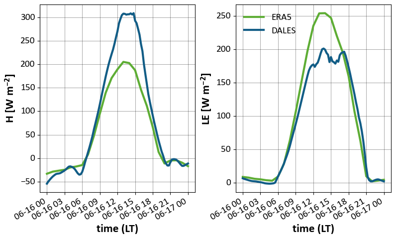
Figure 3 Sensible and latent heat fluxes averaged over domain from ERA5 (green) and DALES (blue).

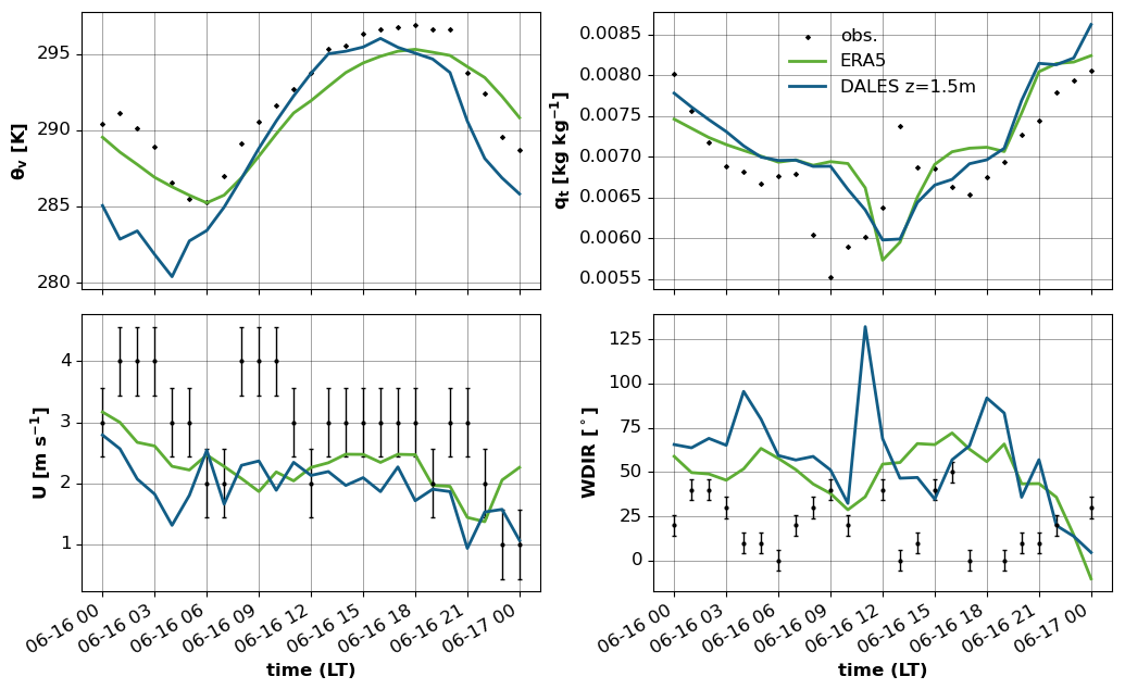
Figure 4 Time series of virtual potential temperature, specific humidity, wind speed, and wind direction from DALES (blue), ERA5 (green), and observations (dots) on 16 June 2022. DALES data are extrapolated to measurement height (1.5 m).

Vertical profiles of virtual potential temperature (θ_v) show the development of a well-mixed convective boundary layer in the morning and the formation of a stably stratified nocturnal boundary layer at night (Fig. 5a). The wind speed in the mixed layer ranges from 4 m s⁻¹ during the daytime to 7 m s⁻¹ in the early morning of 17 June (Fig. 5c). The θ_v profile indicates a boundary layer evolution from 250 m at 06:00 LT to about 1250 m at 12:00 LT and below 200 m during the night (00:00 LT).

Comparison with ceilometer data at Maastricht Aachen airport is shown in Fig. 5d. The colors depict the attenuated backscatter signal of the ceilometer, and the black line is the boundary layer height calculated by DALES. Although the measurement station is approximately 100 km from Eindhoven, the trend should be comparable. The development of the boundary layer calculated from DALES fits the ceilometer data well up to about 21:00 LT, after which the modeled boundary layer height shows a sharp decrease, whereas the ceilometer data show a more gradual decrease, taking about 1.5 h to decrease to its nocturnal value. This is likely related to the evening transition, during which the strength of the convective turbulence decreases, as buoyancy disappears as its driving force, and a shallow nocturnal boundary layer is formed (Darbieu et al., 2015). During this transition, turbulent length scales decrease to sizes that cannot be resolved at the 50 m resolution of our simulations. The much smaller eddies that dominate the evening atmosphere will be of comparable or even smaller scale than the cell size, which means that most of the turbulence is covered by the sub-grid-scale model. Simulations at 25 m resolution (which is the lower bound currently set by the emission downscaling) did not lead to improvements in the representation of the evening transition. A horizontal resolution of ≈ 10 m would be more appropriate to simulate the transition to a stable boundary layer (Beare et al., 2006). In addition to using a finer resolution, applying a different sub-grid model may help to improve the simulation of the transition to a stable boundary layer. For this study, we applied the subfilter-scale turbulent kinetic energy (SFS-TKE) e scheme (Deardorff, 1980), which is the default in DALES. In future studies, the use of a sub-grid model for the simulation of stable nocturnal boundary layers with coarse resolution (Dai et al., 2021) will be explored. At night, boundary layer heights of 0 m are diagnosed due to the use of the maximum $\mathrm{\Delta }{\mathit{\theta }}_{\mathrm{v}}/\mathrm{\Delta }z$ as a criterion. This approach is valid under convective conditions only, when the boundary layer is capped by a clear temperature inversion. Figure C1 shows boundary layer heights from the same simulation diagnosed with different approaches.

In conclusion, the evaluation of the meteorological variables shows that the DALES configuration applied in this study is able to downscale the ERA-5 meteorological situation successfully. As expected, the different LU classification induces slight differences in the latent and sensible heat fluxes. The main caveat is that the collapse of the boundary layer is quite sudden, which will negatively impact the modeled pollutant concentrations as the mixing after the evening rush hour is clearly underestimated.

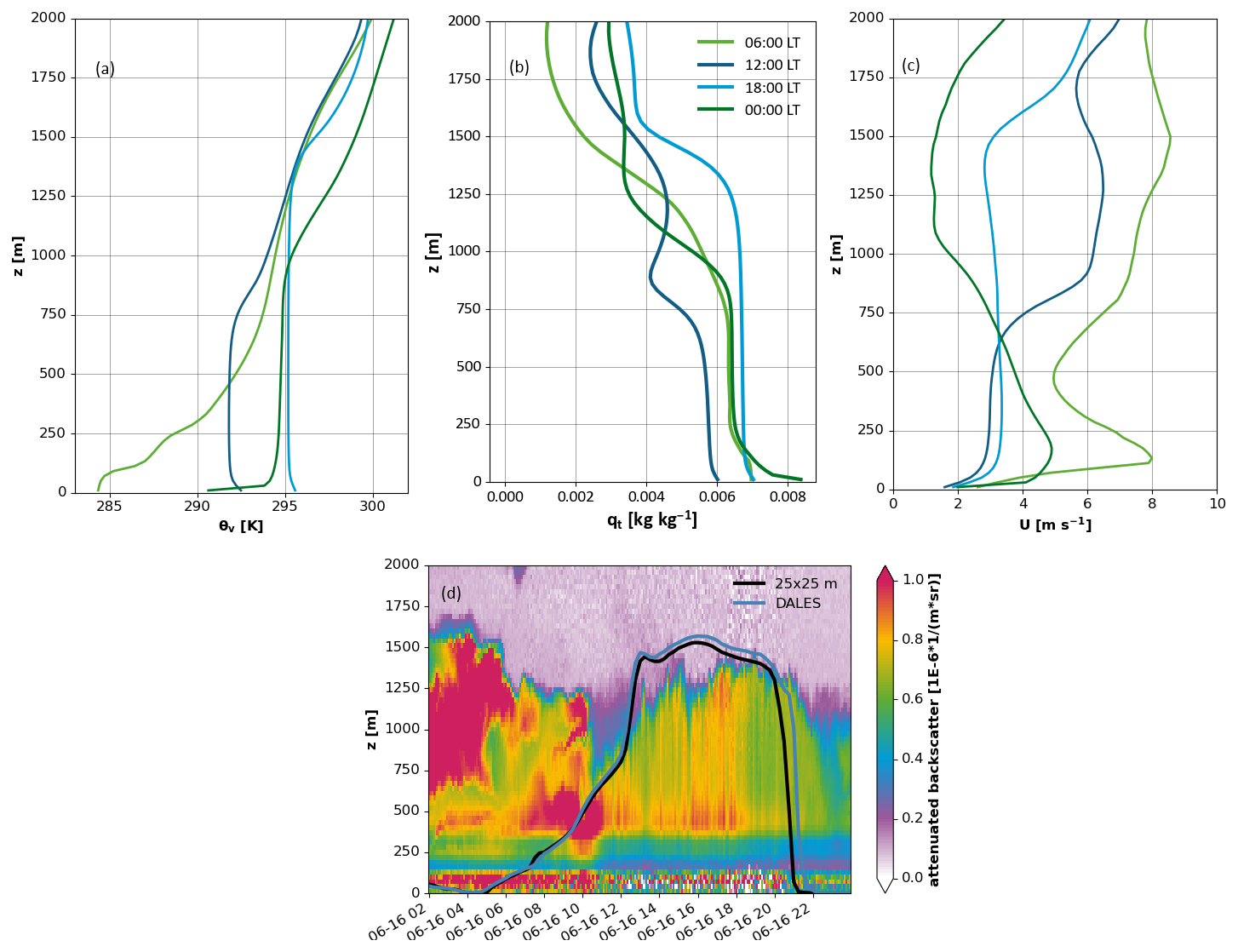
Figure 5 Vertical profiles of domain-averaged virtual potential temperature θ_v (a), total specific humidity q_t (b), wind speed U (c), and boundary layer height and ceilometer backscatter profile on 16 June 2022 (d). The latter includes the simulated boundary layer height for the default simulation (DALES; 50 × 50 m² horizontal resolution) and an additional simulation at 25 × 25 m² resolution.

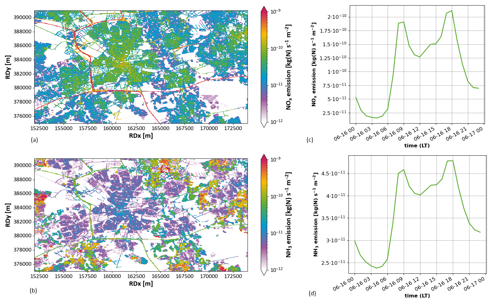
Figure 6 Spatial distribution of NO_x (a) and NH₃ (c) emissions (at 06:00 LT) and the domain-averaged emission time profiles of NO_x (b) and NH₃ (d). Maps are plotted using Rijksdriehoeks (RD) coordinates (EPSG 28992).

3.2 NO_x and NH₃ emissions, dispersion, and deposition

Maps of the downscaled NO_x and NH₃ emissions at a resolution of 50 × 50 m² and their time profiles are shown in Fig. 6. NO_x emissions are assumed to consist of 97 % NO and 3 % NO₂. The maps show the emissions at 06:00 LT, before the morning rush hour. The NO_x emissions range over 3 orders of magnitude with very low values in the rural areas, increasing in the urban areas moving closer to the city center to their maximum values on the highways. The time profile shows two clear peaks during the morning and evening rush hours when the emissions from traffic dominate, intermediate values during the day, and low values at night. As traffic is a relevant source of ammonia in large urban areas (Wen et al., 2023), we can identify the highways as strong emitters of NH₃, in a way similar to NO_x. Some strong agricultural NH₃ sources can also be found in the rural areas on the western, northeastern, and southeastern edges of the domain. The NH₃ emissions show a similar temporal profile as the NO_x emissions, but with values that are about an order of magnitude lower. The time profiles mainly reflect the diurnal cycle in traffic emissions, with rush hour peaks in the morning and at the end of the afternoon (Manders et al., 2017). Diurnal cycles for sectors like industry and agriculture have a more flat profile over the day.

The resulting vertical profile of the mean NO_x concentration over the domain (Fig. 7a) shows a trend similar to the boundary layer development (Figs. 5d, C1). This demonstrates the mixing of the emitted NO_x over the whole boundary layer. The concentration shows a peak near the surface in the morning (09:00 LT) caused by the rush hour emissions (Fig. 6b) and the low boundary layer into which these emissions are mixed (Fig. 5d). A second and much higher peak in the NO_x concentration is simulated in the evening (22:00 LT). This peak coincides with a minimum in the diagnosed boundary layer height and is caused by a lack of mixing simulated by DALES in the evening. Improving this will be a priority for future applications of DALES in air quality and deposition studies. Near the top of the convective boundary, NO_x mixing ratios are diluted due to entrainment of NO_x-poor air from the free troposphere. The NO_x turbulent flux profile shows a positive flux throughout the boundary layer at all times during the simulation. This means that emission and upward mixing dominate over dry deposition and entrainment. This is expected for a tracer with strong sources over the whole domain. In addition, the dry deposition flux of NO_x is significantly lower than the dry deposition flux of NH₃. The highest fluxes are found at 12:00 and 18:00 LT when both emissions and vertical mixing are strong (Fig. 7b).

For NH₃, we find a negative concentration gradient from the surface to the boundary layer background concentration of 2.7 ppb at 12:00, 18:00, and 00:00 LT but a positive gradient at 06:00 LT (Fig. 7c). This positive gradient is caused by dry deposition. In the early morning, the uptake of NH₃ on wet surfaces forms a strong sink, which leads to a net negative NH₃ flux towards the surface (Fig. 7d). Fluxes of both NO_x and NH₃ show a strong divergence, countering the concept of a constant deposition velocity.

The temporal development of the domain-averaged concentrations in the lowest model layer (between 0 and 20 m) (Fig. 8) shows similar trends for the two species. Near-surface concentrations are relatively constant during daytime, with a significant increase in the evening. This increase can be explained by the fast collapse of the boundary layer (Fig. 5d) and by the fact that the emissions from evening traffic are still high, while atmospheric mixing has already subsided.

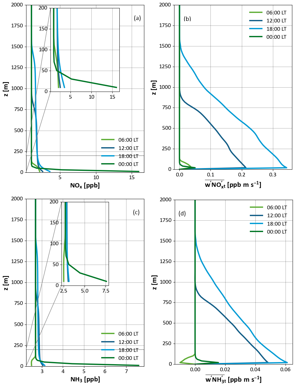
Figure 7 Vertical profiles at different times of NO_x (a) and NH₃ concentrations (c), as well as the total turbulent fluxes of both species (b, d). In (a) and (b) a zoom-in on the lowest 200 m is shown in the inset.

The diurnal cycle of NO_x shows a strong relationship between the concentration and the flux (Fig. 8a), indicating that the deposition flux is mainly driven by the concentration gradient between the atmosphere and the surface. It also shows that during most of the day, the canopy resistance (R_c) is the most important factor that drives the deposition velocity (V_d; Fig. 8c). For NO_x, the R_c mostly follows the stomatal resistance, as shown by the decreasing R_c during daytime. Only during nighttime does the aerodynamic resistance (R_a) play a significant role in determining the deposition velocity. For NH₃, a different picture emerges (Fig. 8b). During nighttime (between 00:00 and 06:00 LT), the NH₃ concentration and deposition are coupled, but during the morning (between 06:00 and 10:00 LT), the concentration increases while the deposition flux decreases. This is driven by an increasing R_c (Fig. 8d). For NH₃, the uptake on wet external surfaces is the most important contribution to the canopy uptake, and this pathway decreases when dew on the leaves evaporates. During daytime (10:00 to 20:00 LT), the concentration and flux remain relatively constant. In the evening (between 20:00 and 00:00 LT), the deposition flux increases due the increased concentration, while the R_c decreases again due to dew formation. The V_d is dampened by the rising R_a. For both species, R_b only plays a minor role in determining the deposition velocities during the whole day.

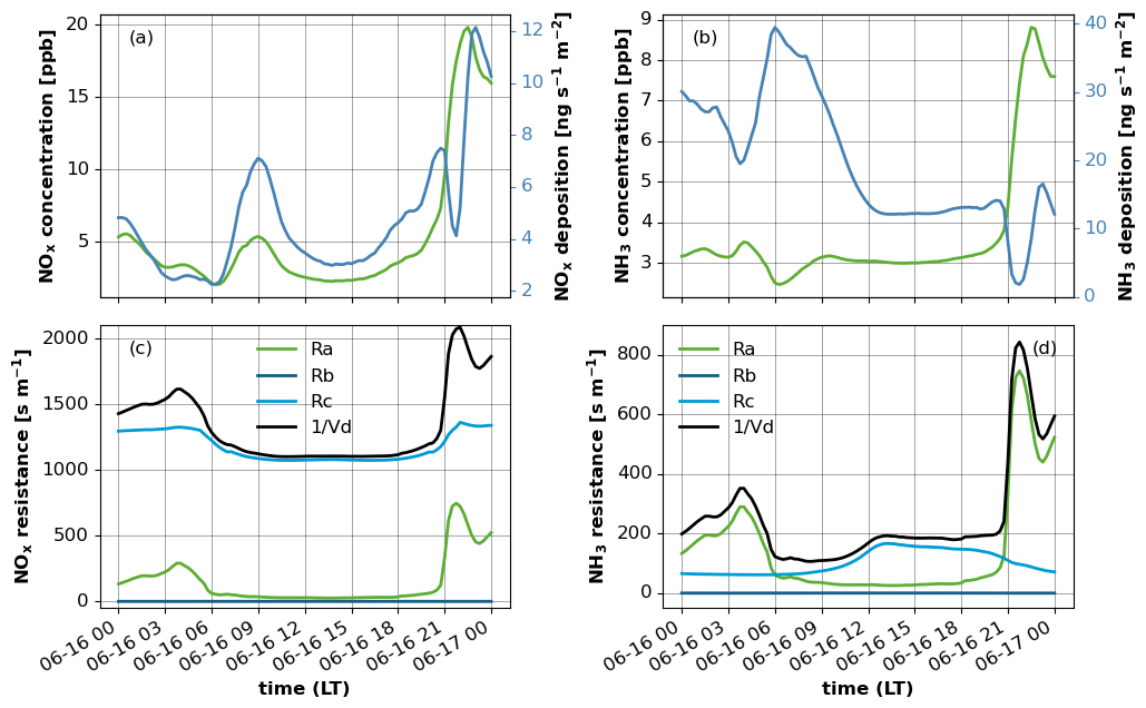
Figure 8 Domain-averaged diurnal cycle of the concentration and deposition flux of NO_x (a) and NH₃ (b) and of the reciprocal deposition velocity ($\mathrm{1}/V_{\mathrm{d}}$) and the aerodynamic (R_a), quasi-laminar (R_b), and canopy (R_c) resistance for NO_x (c) and NH₃ (d).

Figure 9a shows the concentration distribution in the domain at 08:00 LT in the lowest layer of the model. The highways clearly stand out as the main sources of NO_x, producing a local increment of more than 15 µg m⁻³ which is dispersed downwind. In addition, a few other strong sources (mainly industrial) are visible at different locations in the domain. The plumes of NO_x generated by highway traffic can still be discerned visibly from the background at 2–3 km from the source. The emitted nitrogen oxides are carried downwind, undergoing vertical mixing. which causes the near-ground concentrations to become reduced away from the source. The atmospheric mixing depends on the LU adjacent to the highways, as the concentrations trail off at a lower rate over surfaces with low roughness (grass) compared to high roughness (forest). The concept of blending distance can be used to quantify the distance over which emission plumes travel before they are well mixed with the background concentration distribution (Schulte et al., 2022).

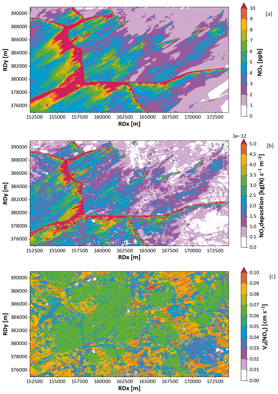
Figure 9 Distribution of NO_x concentration in the lowest layer of the model (z=10 m) (a), distribution of the deposition flux of NO_x (b), and distribution of (c) the deposition velocity of NO_x over the domain at 08:00 LT. Note that NO_x is deposited as NO₂.

The lowest concentrations are found at the east and north border of the domain, and it is the boundary conditions imposed on the model (see Sect. 3) that explain this. DALES currently does not yet support open boundary conditions. Instead, in the present simulations, we imposed a constant concentration on the boundaries (1 ppb, amounting to approx. 1.3 µg m⁻³), which ignores the presence of sources outside the domain but provides a realistic background concentration for NO_x. DALES is currently being extended by implementing the possibility to nest a calculation in a bigger domain, enabling the use of boundary conditions originating from a parent domain from DALES or a regional-scale atmospheric model (Liqui Lung et al., 2024). This will enable setting realistic boundary conditions with a more accurate background concentration and incorporating the effect of plumes generated outside the domain.

The concentration difference between the lowest layer of the atmosphere and the compensation point (which is 0 for NO_x) is the driving force of the deposition flux (Fig. 9b). The deposition velocity (Fig. 9c) is the conversion factor between this concentration difference and the deposition flux. Note that we treated NO_x as NO₂ in our deposition calculations, since in the atmosphere, NO emissions are quickly chemically converted to NO₂. Due to its LU dependence, the deposition velocity shows a clear footprint of the LU map. Grassland and open fields show low values (0.04 cm s⁻¹) for deposition velocity, increasing a little for urban areas (0.06 cm s⁻¹) and reaching maximum values over forests (0.08 cm s⁻¹). For NO_x these differences are mainly due to the difference in roughness length between the LU types.

The NH₃ concentration field at 08:00 LT mainly reflects the emissions from agriculture, and hence we find concentration maxima near farm locations at the northern and western edges of the domain (Fig. 10a). Also, the areas downwind of the highways show elevated concentrations. The atmospheric lifetime of a primary air pollutant and thus its traveling distance are governed by an intricate balance between height of emission, advection, and turbulent transport, as well as the removal rates by dry and wet deposition. Specifically for reactive and water-soluble pollutants emitted close to ground level, like NH₃, the travel distance is shortened by deposition fluxes. This means that species are allowed to travel further over land with a low deposition flux, like grassland and urban areas. Forests are effective at shortening travel distances.

The modeled NH₃ deposition fluxes are about an order of magnitude larger than those of NO_x (Fig. 10b). Similarly to NO_x, the influence of LU is clearly visible in the deposition flux NH₃: the smallest fluxes are calculated in urban areas and water bodies, whereas the largest deposition fluxes are found over forest areas. The striking features are modeled near the transition from agricultural land (pastures and cropland) to forest in the northeastern part of the domain (indicated by the box in Fig. 10b): here, plumes enriched with NH₃ are advected from a smooth to a rough surface. Over the rough surface, turbulent exchange is enhanced, which leads to rapid deposition of NH₃. Further into the forest the deposition fluxes become smaller than near the transition. This shows that a high-resolution, turbulence-resolving model like DALES is uniquely suited to simulate this kind of small-scale feature, in which the interactions between the turbulent transport and the change in local LU together determine the deposition flux.

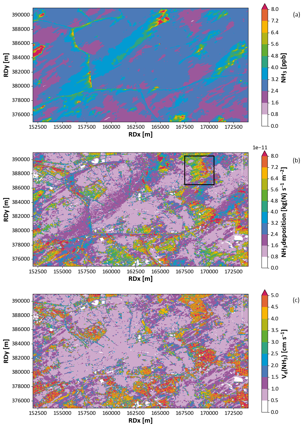
Figure 10 Distribution of NH₃ concentration in the lowest layer of the model (z=10 m) (a), distribution of the deposition flux of NH₃ (b), and distribution of (c) the deposition velocity of NH₃ over the domain at 08:00 LT.

A limitation of our study is the fact that we ignore possible effects of chemistry and aerosol formation on the deposition of NO_x and NH₃. Under atmospheric conditions, NO_x will be partially converted into HNO₃, which deposits more readily than its precursor and which can be neutralized with NH₃ to form ammonium nitrate aerosol. DALES has been used before to study the effects of turbulent mixing on the phase transition of ammonium nitrate. Aan de Brugh et al. (2013) found that aerosol-poor air is transported upward from the surface and aerosol-rich air is transported from high altitudes downward, since equilibrium between the gas and aerosol phase is not instantaneous. Further, Barbaro et al. (2015) found large deposition velocities for nitrate due to outgassing near the surface. Finally, a study with another LES code concluded that the effective Henry’s law constant is a critical factor for parameterization of dry deposition of gas-phase species in a street canyon (Lin et al., 2024). Taking into account the effects of gas-phase chemistry and gas–aerosol partitioning will have considerable impacts on the calculated deposition fluxes. We aim to cover the effects of a full coupling between emissions, chemistry, partitioning, and turbulent transport in a follow-up study.

4 Evaluation against observations at Cabauw

To ensure the validity of the deposition fluxes calculated by DALES, an evaluation against measurements is urgently needed. However, the possibilities for such an evaluation are limited by the availability of reliable flux measurements (Wintjen et al., 2022). In this section, we therefore provide a limited evaluation for a single day. Because no observations of deposition fluxes are available for Eindhoven, we evaluate DALES against observations at the Cabauw experimental site in the Netherlands (51.97° N, 4.93° E). This site is in almost flat terrain consisting primarily of grassland. Input data for DALES calculations were acquired in the same way as for the Eindhoven case (Sect. 2.4 and 2.5). The concentration and deposition flux of NH₃ were calculated on 25 September 2021 (dry day, SSW wind turning E, 2–4 m s⁻¹, 15–21 °C, 70 % RH during the day, 90 % at night). Measurements of NH₃ concentration and deposition flux for this day were acquired, as part of the RITA-2021 campaign, by a Healthy Photon HT8700E open-path ammonia analyzer (eddy covariance flux analyzer) and the RIVM miniDOAS 2.2D (differential optical absorption spectroscopy) instrument (Swart et al., 2023).

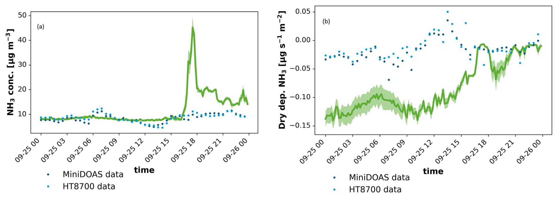
Figure 11 Modeled and measured concentration (a) and deposition flux (b) at Cabauw compared to measurement data by the miniDOAS and HT8700. DALES results are shown by the green line, with the shades indicating the standard deviation of the DALES output for grid cells within a radius of 100 m around the data sampling location.

Figure 11 shows the NH₃ concentration and deposition flux during the day. The predicted concentration was around 9 µg m⁻³, which is comparable to the measured concentrations. The predicted concentration peak in the evening does not reflect the measured data because of the transition from an instable to a stable boundary layer that is not yet covered well by DALES. The deposition flux is overestimated by the model in the morning and afternoon, but it settled to a value around the measurement data after the wind subsided and its direction changed in the evening. DEPAC is known to overestimate deposition fluxes, particularly during early morning hours (Jongenelen et al., 2025). One cause for this overprediction can be the overestimation of LAI in DEPAC. The value for grassland is estimated at 3 on 25 September 2021, whereas the MODIS satellite LAI measurements show values between 1 and 2 at Cabauw in that period. A further evaluation over other land use types would be commendable, but that depends on the availability of reliable flux measurements of reactive nitrogen, which are sparse (Wintjen et al., 2022).

5 Conclusions

Studying the fate of reactive nitrogen compounds in a complex landscape, while accounting for the interplay between dispersion, chemistry, and deposition processes, requires a detailed model setup at very high spatial and temporal resolution. We have taken the first steps in preparing the Dutch Atmospheric Large Eddy Simulation (DALES) model for such realistic applications. As a first step we successfully integrated the dry deposition module based on DEPAC in DALES, supported by a flexible land use definition. Also, we provided high-resolution emissions of NO_x and NH₃ for the model system.

In a case study for the Eindhoven region we found that DALES is able to reproduce the main features of the boundary layer development and diurnal cycle of local meteorology well, with the exception of the evening transition. DALES calculates the dispersion and deposition of NO_x and NH₃ in great spatial detail, clearly showing the influence of local land use patterns on removal efficiencies and mixing characteristics. This shows the promise of the model for deposition studies in complex landscapes. To further develop the system for realistic applications we are working on detailing the emissions on the required scale, the integration of gas phase chemistry, inorganic aerosol formation, and the accommodation of open boundary conditions. In particular regarding emissions, the adoption of a dynamic scheme will reduce the uncertainty of emission fluxes and local concentration estimates.

Appendix A: LSM and DEPAC parameters

Table A1 Parameters for the HTESSEL land surface model (ECMWF, 2021; Balsamo et al., 2009).

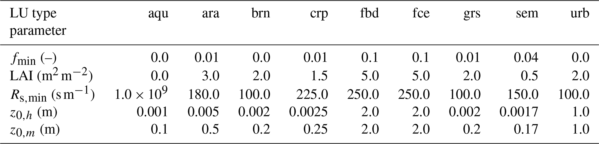
Table A2 Parameters for the deposition model (Van Zanten et al., 2010).

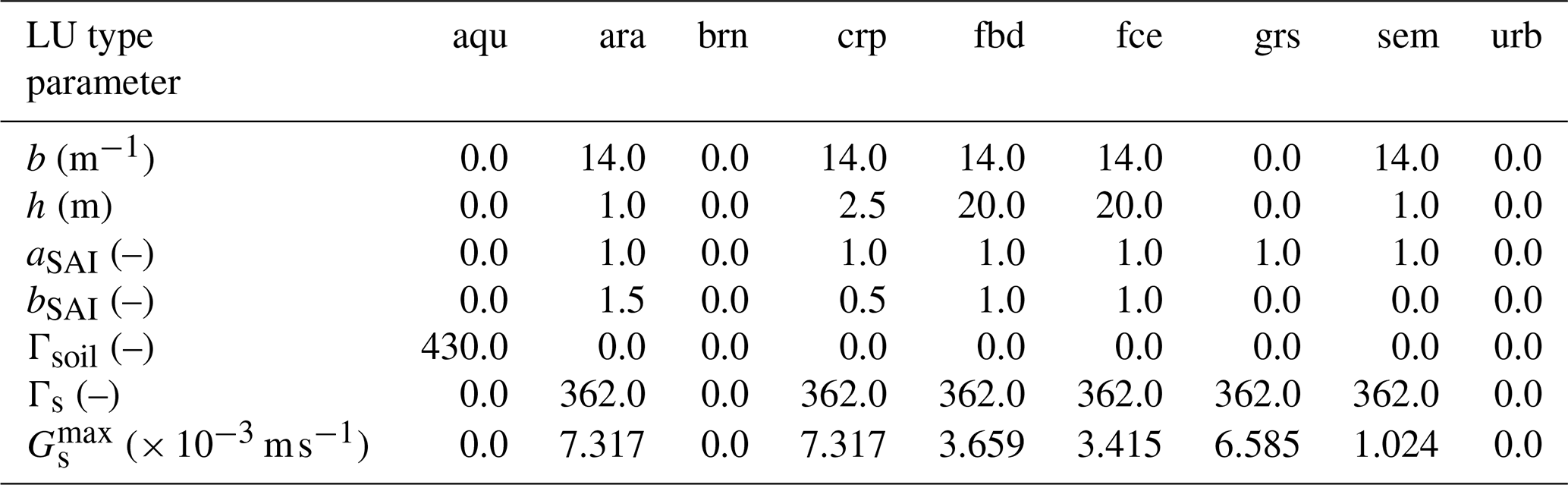
Table A3 Model parameters for soil resistance R_soil (s m⁻¹) (based on Erisman et al., 1994).

Appendix B: Land use translation

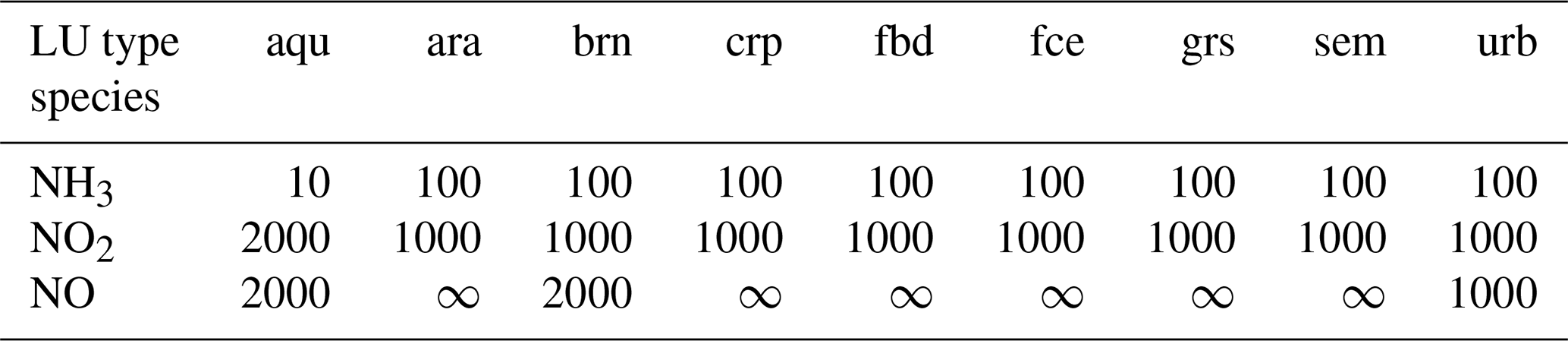
Table B1 Translation table of TOP10NL land use types (in Dutch) to DEPAC land use types.

Appendix C: Boundary layer height diagnostics

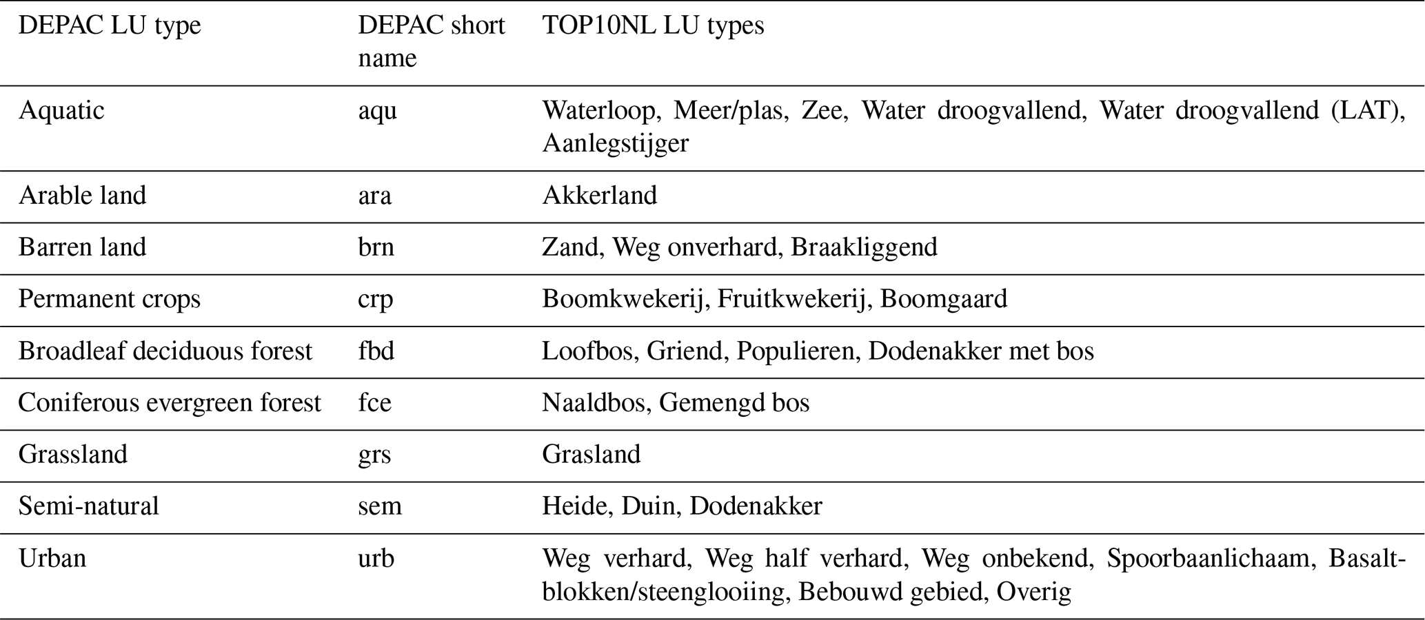
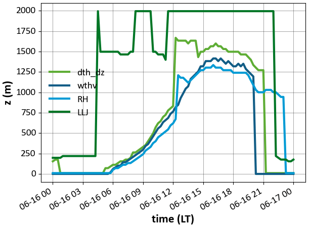
Figure C1 Boundary layer height from DALES as diagnosed by four different methods: heights of the maximum $\mathrm{\Delta }{\mathit{\theta }}_{\mathrm{v}}/\mathrm{\Delta }h$, minimum value of $\stackrel{\mathrm{‾}}{w^{\prime }{\mathit{\theta }}_{\mathrm{v}}^{\prime }}$, maximum value of RH, and low-level jet.