PyGLDA: a fine-scale python-based global land data assimilation system for integrating satellite gravity data into hydrological models

Data assimilation (DA) of time-variable satellite gravity observations, such as those from the Gravity Recovery and Climate Experiment (GRACE), GRACE Follow-On (GRACE-FO), and future gravity missions, can be used to constrain simulations of the vertical sum of water storage in Global Hydrological Models (GHMs). However, current DA implementations of these Terrestrial Water Storage (TWS) changes are often performed at regional scales or, if applied globally, at low spatial resolutions. This limitation is primarily due to the high computational demands of DA and numerical challenges, such as instabilities in covariance matrix inversion. To fully exploit the potential of satellite gravity observations and the high spatial resolution of GHMs, we developed PyGLDA, an open-source Python-based system that enables fine-scale and computationally efficient global DA. The key innovations of PyGLDA include (1) a global patch-wise DA approach using domain localization and neighboring-weighted global aggregation and (2) seamless compatibility between basin-scale and grid-scale DA implementations. PyGLDA represents a significant functional improvement over previous DA systems, offering wide-ranging and flexible options for user-specific applications. The modular structure of the system allows users to customize water storage compartments, modify observation representations, and potentially select different GHMs. This paper provides a comprehensive description of PyGLDA and its application in a case study of the Danube River Basin, along with a demonstration of global DA, where experiments involve integrating monthly GRACE TWS fields (2002–2010) with the daily W3RA water balance model at 0.1° spatial resolution.

1 Introduction

Accurate monitoring of the global water cycle is essential to understand natural climate change, as well as human water resource management (Rodell et al., 2018). However, measuring global changes in Terrestrial Water Storage (TWS) – which represents the total vertical sum of water stored on land, including ice, snow, wetlands, lakes, rivers, soil moisture and groundwater – has long been a challenge (Rodell and Reager, 2023). This difficulty arises from the vast spatial coverage required (approximately 150 million km² of the global land area) and the lack of comprehensive observational data for different hydrological components. In situ measurements of key variables, such as groundwater, are often spatially and temporally limited, subject to political constraints, and prone to data gaps and systematic errors. These factors reduce their suitability for large-scale hydrological studies (Li et al., 2019).

To address these challenges, Global Hydrological Models (GHMs) have been developed to simulate the spatially distributed hydrological response to weather and climate variations, as well as human water use. Most GHMs are conceptually or physically based, and one can see Sutanudjaja et al. (2018) for an extensive list of existing GHMs. These models operate at various spatial resolutions, ranging from coarser scales (e.g., 0.5°×0.5° for WaterGap, Müller Schmied et al., 2021) to finer resolutions (e.g., 0.01°×0.01° for the hyper-resolution PCR-GLOBWB, Hoch et al., 2023). Despite their advancements, these models often struggle to realistically simulate certain water storage and flux processes due to oversimplified representations of natural processes or a lack of constraints on the temporal variability of some components, such as groundwater and human interventions. This issue persists in most GHMs (Scanlon et al., 2018; Mehrnegar et al., 2020), although some models may perform better than others in specific river basins. Recent efforts have aimed to improve the representation of certain components, such as groundwater processes, to more accurately simulate groundwater levels and surface–groundwater interactions. However, significant modeling challenges persist (see Niu et al., 2007; de Graaf et al., 2017; Decharme et al., 2019). Furthermore, calibrating model parameters to better capture local water variability remains a major challenge, which requires innovative observational and calibration techniques (Schumacher et al., 2018).

Since 2002, satellite observations of time-variable gravity changes have been available through the US-German Gravity Recovery and Climate Experiment (GRACE) mission (Tapley et al., 2004). By analyzing these data, researchers can estimate global TWS changes with reasonable precision (Landerer and Swenson, 2012). During the past two decades, GRACE and its Follow-On mission (GRACE-FO; Landerer et al., 2020) have contributed significantly to hydrological and meteorological studies. These satellite-based TWS observations have been used to close the global water budget (e.g., Sheffield et al., 2009; Castle et al., 2016), estimate groundwater depletion (e.g., Scanlon et al., 2012; Voss et al., 2013; Castellazzi et al., 2016), analyze droughts and flood potential (e.g., Gouweleeuw et al., 2018; Forootan et al., 2019), validate and constrain hydrological models (e.g., Ngo-Duc et al., 2007; Eicker et al., 2016; Mehrnegar et al., 2020, 2023). However, despite its advantages, the GRACE-derived TWS anomalies (abbreviated as TWS hereinafter) are limited by coarse spatial and temporal resolution (∼330 km or 3°×3° on a monthly basis) due to the presence of considerable correlated noise (Kusche et al., 2009; Chen et al., 2022; Yang et al., 2024b).

To introduce realistic variability from observations into model simulations, Data Assimilation (DA) techniques have gained significant attention. In particular, DA of GRACE-based TWS observations can enhance the temporal, horizontal, and vertical disaggregation of the estimated TWS signal (Zaitchik et al., 2008; Schumacher, 2016). GRACE data provide unique constraints on model-based water storage estimates that cannot be obtained through other observational techniques. Numerous studies have demonstrated the effectiveness of DA with GRACE in improving TWS simulations and its individual components, particularly at regional and basin scales (Eicker et al., 2014; van Dijk et al., 2014; Schumacher et al., 2016; Girotto et al., 2016; Khaki et al., 2017; Tian et al., 2017). More recently, there has been a growing interest in implementing GRACE-TWS DA on a global scale to better capture the global water cycle (Li et al., 2019; Felsberg et al., 2021; Gerdener et al., 2023; Forootan et al., 2024).

However, few studies have achieved high-resolution global DA of GRACE-TWS and hydrological models. Li et al. (2019) reported a 0.25° global DA resolution, which, to the best of our knowledge represents the highest resolution achieved so far. Although the value of high-resolution hydrological modeling (for example the resolution of 0.1°) has been widely acknowledged (Benedict et al., 2017; Sutanudjaja et al., 2018; Springer et al., 2019), the implementation of high-resolution global DA remains highly challenging due to numerical instabilities and computational constraints. The latter, in particular, poses a critical challenge, often rendering traditional DA frameworks impractical for large-scale applications. Additionally, none of the existing global DA implementations for GRACE-TWS have made their software publicly available, limiting transparency and reproducibility within the scientific community.

In this article, we introduce PyGLDA, the first open-source and Python-based Global Land Data Assimilation (GLDA) system designed to address the challenges of high-resolution global DA. PyGLDA enables the integration of satellite-based TWS observations from GRACE, GRACE-FO, and likely future gravity missions (Daras et al., 2023) with GHMs. In this version, W3RA model (van Dijk, 2010) is selected as the GHM. The software is a key outcome of the DANSK-LSM project (https://aaugeodesy.com/dansk-lsm/, last access: 1 June 2024) and will be expanded in the future for multi-sensor hydrological DA applications. Unlike previous studies, PyGLDA introduces a fully restructured DA framework to efficiently and stably implement high-resolution global DA at 0.1° spatial resolution and a daily time step. The system includes several key innovations:

• A unified framework for both basin-scale and grid-scale DA, where the area to be covered is defined as a “basin” and each grid cell acts as a “sub-basin”, allowing for flexible spatial configurations via standard shapefiles;

• A novel approach for transitioning from regional DA to global DA, achieved through domain localization and neighboring-weighted aggregation algorithms;

• The ability to compute spatial covariance of GRACE-based TWS observations, enabling full covariance matrices for sub-basins and grids, which improves DA reliability by considering spatial correlations;

• Flexible choice of the grid/sub-basin GRACE-TWS observations to be assimilated into GHMs, e.g., from 1 to 5° with an increment of 0.5°;

• A range of perturbation strategies for generating ensemble members, allowing users to select which forcing data and which model parameters are to be perturbed following which noise distribution (Gaussian or Triangle distribution, as well as additive or multiplicative noise);

• The Ensemble Kalman filter (EnKF similar to Schumacher, 2016), and an Ensemble Kalman Smoother (EnKS) that optimally desegregates monthly increments to daily ones (similar to Tian et al., 2017), are implemented as mergers.

The architecture of the code includes the following features:

• A flexible modular structure to decouple PyGLDA into three individual modules: (1) GHM, (2) GRACE processing, and (3) DA integration. This choice is made to make it possible to develop/modify/replace any individual module;

• PyGLDA is implemented in object-oriented Python, making it accessible and easy to use, while maintaining computational efficiency comparable to C$++$, Fortran, and MATLAB. The Python translation of the W3RA model (van Dijk, 2010) is distributed as well;

• Cross-platform compatibility, allowing installation on Windows, Linux, and High Performance Computing (HPC) clusters; Configurable settings via JSON files, enabling users to adjust parameters and options without modifying the source code; Efficient data management, using the modern HDF5 format for handling large spatial-temporal datasets.

The paper is structured as follows. In Sect. 2, we describe the data required for PyGLDA. In Sect. 3, a detailed description of employed GHM and the development of PyGLDA is presented. Section 4 introduces some application examples to demonstrate the effectiveness and flexibility of PyGLDA. The current limitations of PyGLDA are summarized in Sect. 5. Finally, conclusions and outlooks are demonstrated in Sect. 6.

2 Data

2.1 Masks

PyGLDA defines various data masks to facilitate the management of DA processes. A flexible combination of these masks allows users to conduct a wide range of studies, whether at the basin scale or grid scale, and whether DA is performed globally or locally. The system supports five primary mask types, which must be properly configured: (1) land mask that identifies grid points at land; (2) data mask that indicates areas where forcing fields and model parameter fields are available; (3) region mask that specifies where one wishes to run GHM; (4) basin mask that defines where one wishes to perform DA; (5) observation mask that represents sub-basins or grid cells where observational data are assimilated within the DA process. PyGLDA includes default options for the land mask and data mask, but users must define the region mask, basin mask, and observation mask using a standard shapefile format (.shp). This approach ensures flexibility and adaptability, allowing users to tailor PyGLDA to their specific research needs.

2.2 Meteorological forcing field

So far, only ERA5-land reanalysis (Hersbach et al., 2020) data has been integrated into PyGLDA. However, this does not mean that the implementation is restricted to this forcing field. Instead, one can easily modify the interface module to load other meteorological forcing data. In the current PyGLDA, the ERA5-land at a native (also its highest) resolution of 0.1° is required to run W3RA (as an example), which includes the daily precipitation, the maximal/minimal temperature and the surface solar radiation. In particular, PyGLDA provides a function to download these forcing data from the ECMWF (European Centre for Medium Range Weather Forecast) website automatically, which one can use to keep the forcing field up-to-date. In addition, an up(or down)-scaling of forcing fields can be done with the official “metview” package (from ECMWF, https://metview.readthedocs.io/en/latest/, last access: 11 April 2024) integrated in PyGLDA, if one wishes to run PyGLDA at a different spatial resolution.

2.3 Parameters and climatologies

The parameters and climate input data are originally distributed along with the employed GHM, i.e., W3RA, which has an original resolution of 0.5°. PyGLDA provides a finer resolution of 0.1° as a default option. For a detailed review of the definition of these parameters and climatological resources, one can refer to the W3RA technical document (van Dijk, 2010).

2.4 GRACE level-2 product and its covariance matrix

In PyGLDA, the monthly GRACE-based TWS is computed from standard Level-2 gravity field products, which are expressed in terms of spherical harmonic coefficients up to degree/order 60 or 96 (Yang et al., 2017). These Level-2 products are provided by three official data centers, i.e., CSR (Center for Space Research from the University of Texas at Austin, Texas, USA), GFZ (GeoForschungsZentrum, Potsdam, Germany) and JPL (Jet Propulsion Laboratory, USA). Additionally, to generate realistic perturbations for GRACE-based TWS, PyGLDA requires the full error covariance matrix of the Level-2 products. However, this information is not included in the official Level-2 products. To overcome this limitation, PyGLDA uses ITSG-2018 temporal gravity field solutions (Kvas et al., 2019; Mayer-Gürr et al., 2018), which offer key advantages: (i) access to the full error covariance matrix; and (ii) better quality than official products due to the additional background model uncertainty considered (Kvas and Mayer-Gürr, 2019; Meyer et al., 2019).

3 Model description

3.1 Structure

PyGLDA consists of three core scientific modules: (1) GRACE processing, (2) W3RA model, and (3) DA, each of which is described in detail below. Additionally, PyGLDA includes three supporting modules: (4) a postprocessing module for data analysis and visualization, (5) a flow control module that integrates the necessary sub-modules into a streamlined processing chain for specific studies, and (6) an auxiliary module for processes outside DA, e.g., downloading forcing fields and formatting output. Figure 1 provides an overview of the structure of PyGLDA, illustrating the interaction between these modules.

Figure 1 An overview of PyGLDA structure that mainly consists of three modules: (a) GRACE processing, (b) W3RA GHM (van Dijk, 2010) and (c) Data Assimilation (DA).

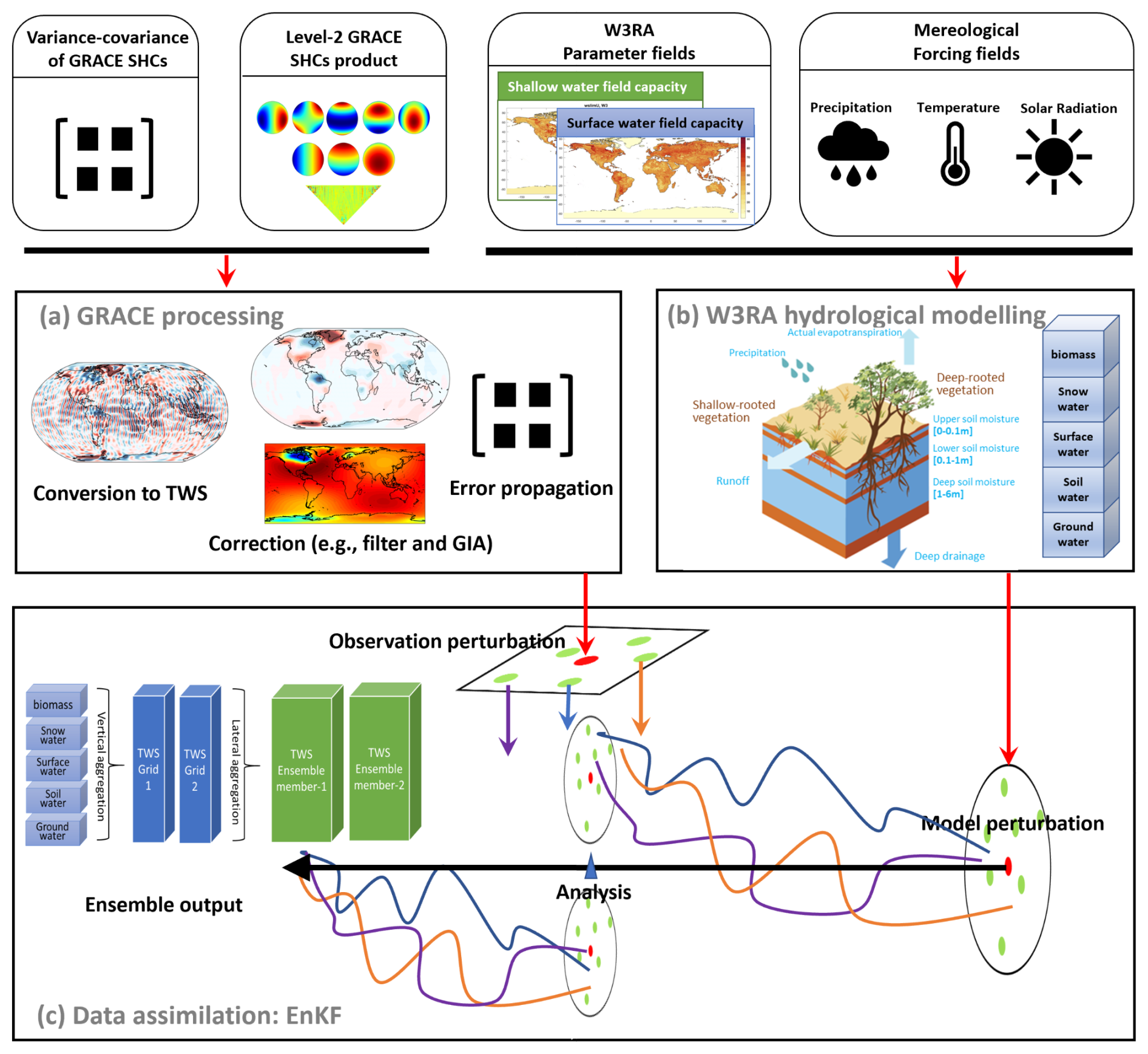
GRACE processing

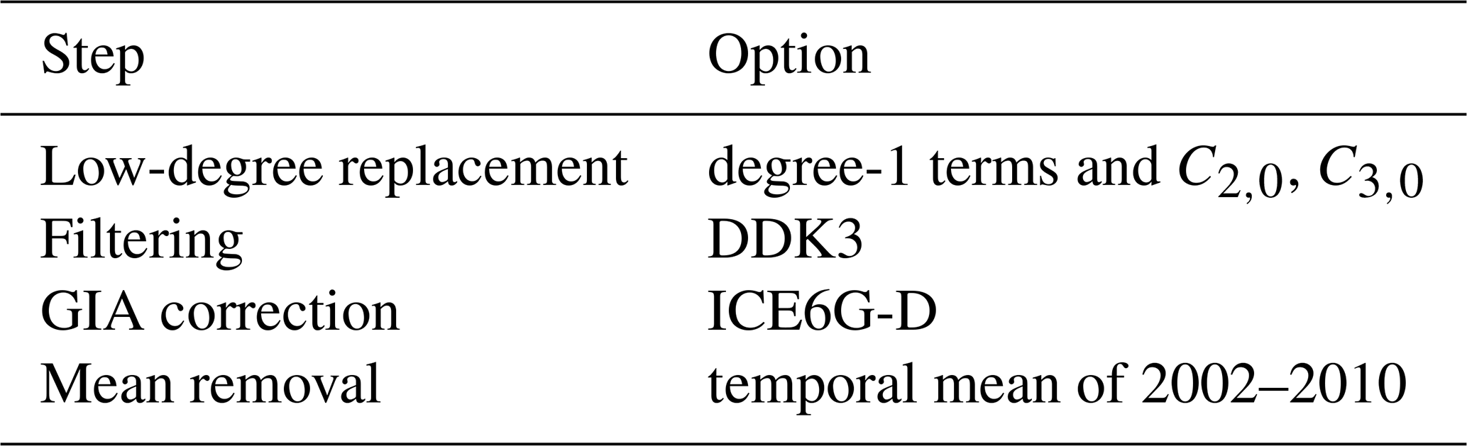
This module is responsible for conversion, correction and propagation of GRACE Level-2 data and its associated uncertainty. By default, GRACE Level-2 products are distributed as geopotential spherical harmonic coefficients (SHCs), which must be transformed into physically meaningful variables, such as gridded TWS anomalies, for use in DA. This transformation, known as conversion, is performed using the harmonic synthesis approach (Wahr et al., 1998). Furthermore, GRACE data contain considerable noise due to imperfect background models (Yang et al., 2021; Zhou et al., 2023) and instrument noise (Yang et al., 2018; Patel, 2020; Yang et al., 2022a). Therefore, a series of corrections is applied to ensure the extraction of a desired signal, including low-degree coefficient replacement (e.g., Loomis et al., 2020), de-correlation and filtering (e.g., Swenson and Wahr, 2006; Kusche, 2007; Klees et al., 2008; Horvath et al., 2018), spatial leakage correction (e.g., Chen et al., 2015; Vishwakarma et al., 2018), Glacial Isostatic Adjustment (GIA) removal (e.g., Richard Peltier et al., 2018). PyGLDA selects and implements the most widely used correction strategies, see Table 1. However, be aware that Table 1 is not exhaustive; many more corrections such as the ellipsoidal correction (e.g., Yang et al., 2022b) are also implemented. Furthermore, to ensure an optimal balance between observational and model-derived water storage estimates, the GRACE-TWS uncertainty must be properly quantified. PyGLDA achieves this through Monte Carlo propagation of the full error covariance matrix from the SHC domain to the gridded (or basin-averaged) TWS domain (Wahr et al., 2006; Boergens et al., 2022; Yang et al., 2024a). Given its independent functionality, all GRACE processing related tasks have been integrated into a standalone toolkit called SaGEA, which is also Python-based and open source (Liu et al., 2025). SaGEA can be seamlessly coupled to PyGLDA.

Swenson et al. (2008)Loomis et al. (2020)Loomis et al. (2020)Swenson and Wahr (2006)Chen et al. (2006)Kusche (2007)Jekeli (1981)Han et al. (2005)Zhang et al. (2009)Chen et al. (2015)Wahr et al. (1998)Klees et al. (2007)Longuevergne et al. (2010)Landerer and Swenson (2012)Vishwakarma et al. (2018)Richard Peltier et al. (2018)A et al. (2013)Caron et al. (2018)

Table 1 An overview of the available correction options in PyGLDA's GRACE processing toolkit, see Liu et al. (2025) for more details.

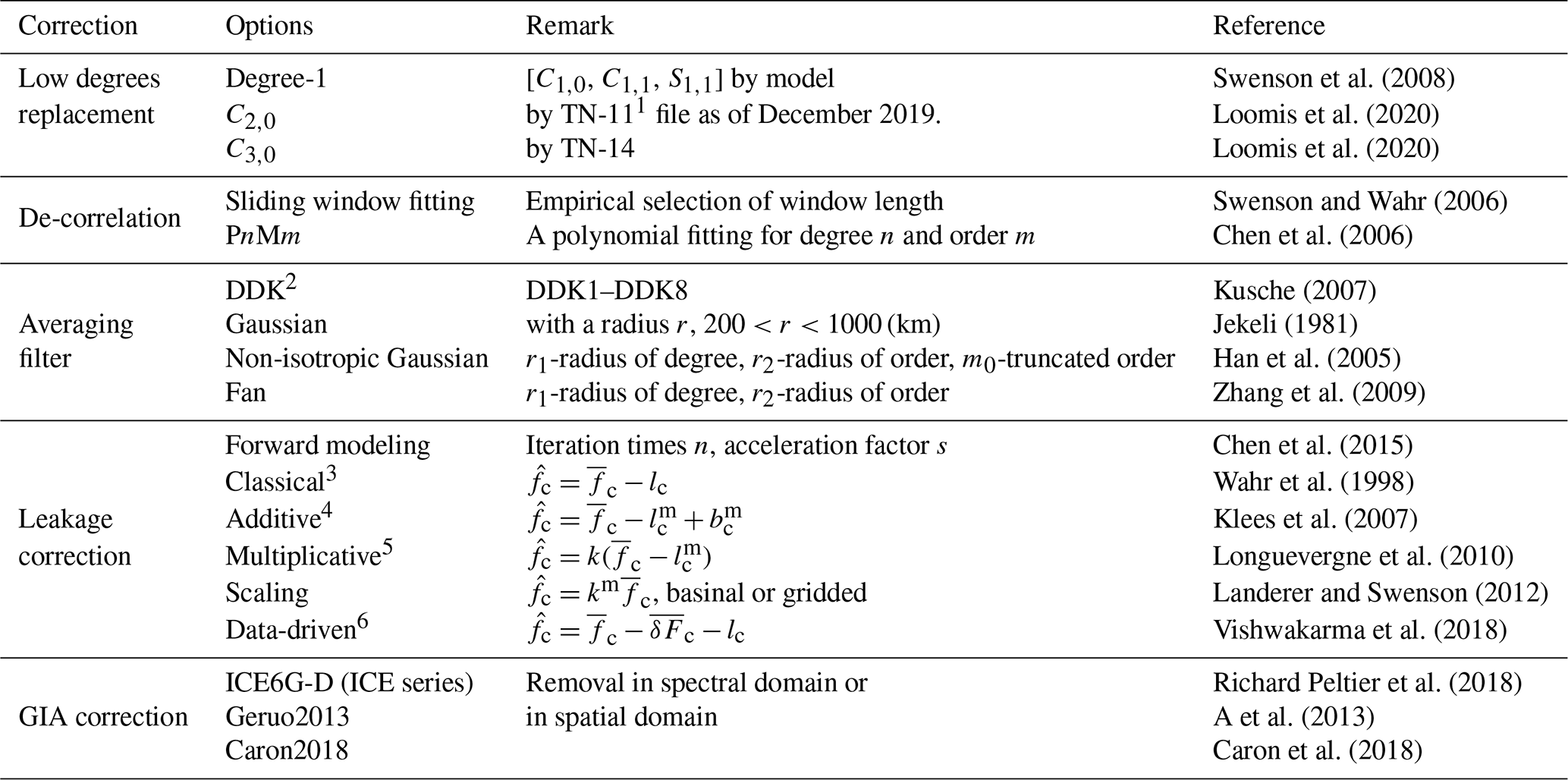
¹ The Technical Note (TN-XX) files are provided along with the official GRACE products. ² DDK is actually a de-correlation and averaging filter (Kusche et al., 2009). ³ where ${\widehat{f}}_{\mathrm{c}}$, ${\stackrel{\mathrm{‾}}{f}}_{\mathrm{c}}$ denote the signal after and before correction; and l_c indicates the spatial “leakage”. ⁴ where b_c indicates the “bias”; and the superscript “m” indicates that a hydrological model is required. ⁵ where k is the derived scaling factor. ⁶ where ${\stackrel{\mathrm{‾}}{\mathit{\delta }F}}_{\mathrm{c}}$ indicates the deviation integral.

W3RA GHM

W3RA is an open-source and global realization of the AWRA-L hydrological model (Australian Water Resources Assessment System, version 0.5) (van Dijk, 2010). It is a grid-based one-dimensional water balance model that represents water storage and flows from soil, groundwater, and surface water. The model employs well-established equations to describe radiation, energy, and water balance processes, requiring minimal meteorological input, including daily gridded precipitation, incoming shortwave radiation, and daytime temperature (typically estimated from minimum and maximum temperature). Although its publicly available version is implemented at 0.5° resolution, we have adapted W3RA to 0.1° resolution to align with the available high resolution meteorological data sets (Mehrnegar et al., 2021). However, a limitation of the current model version is its simplified assumption of lateral water redistribution, which reduces reliability in areas influenced by irrigation, inundation, or groundwater inflows (van Dijk, 2010). This limitation highlights the importance of incorporating GRACE-TWS observations via data assimilation. The original W3RA model was released as an open-source MATLAB script, but it has been fully translated into Python and integrated into PyGLDA. Extensive validation tests across different study areas and forcing datasets confirm that the Python implementation maintains numerical precision and computational efficiency comparable to the original MATLAB version. Furthermore, previous studies have demonstrated the capability of W3RA to capture global water storage variability, making it a suitable choice for integration into PyGLDA (Schellekens et al., 2017; Mehrnegar et al., 2020).

Data Assimilation (DA)

This module consists of four main steps, which are perturbation, initialization, forecast, and analysis. Since Ensemble Kalman Filter (EnKF) and Ensemble Kalman Smoother (EnKS) are selected as our merger in PyGLDA, proper perturbation of both model and observations is required. In PyGLDA, model perturbations – specifically for parameters and forcing fields – can be generated using additive or multiplicative noise, following a Gaussian or triangular distribution (Schumacher, 2016). In contrast, perturbations for GRACE-TWS observations are generated from its full error covariance matrix of the GRACE data. Be aware that the perturbation of the initial field (state vector) is currently not considered in PyGLDA due to its limited impact on the DA of land water (Reichle and Koster, 2003). The initialization step involves a spin-up phase, where the W3RA model is run for at least two years without perturbations, ensuring a stable and physically meaningful initial state. In the forecast step, the model evolves forward on a daily timescale until the next observation becomes available. Finally, in the analysis step, observational data and model forecasts are combined to update the state variables for the past month, following the standard EnKF or EnKS framework; see Appendix A for details.

3.2 DA workflow and parallel computation

State-of-the-art sequential DA methods are widely used in hydrological applications, with Kalman filter-based approaches gaining significant attention due to their relatively straightforward matrix implementation (Schumacher, 2016). The classical Kalman filter assumes that all probability distributions involved in the system are Gaussian and provides algebraic formulations for updating the mean and covariance matrices under the assumption of a linear system. However, maintaining a full covariance matrix is computationally impractical for high-dimensional systems. To address this problem, the EnKF was developed, representing the probability distribution of the system using an ensemble of state vectors rather than an explicitly stored covariance matrix. This approach enables a Monte Carlo approximation of the Bayesian update, where the accuracy of the covariance estimate depends on the number of ensemble members. Since there is no universally optimal ensemble size, PyGLDA allows users to customize the number of ensemble members through a JSON-based configuration file; see Appendix B for details. We recommend an ensemble of 30 members to balance computational efficiency and accuracy (Schumacher et al., 2016, 2018).

In PyGLDA, the processing steps (including perturbation, model forecast, state analysis, and data management) for each ensemble member are completely independent of the others. This independence makes PyGLDA highly suitable for parallel computing, allowing full utilization of CPU resources. In PyGLDA, each ensemble member is assigned to a separate computational thread, significantly improving efficiency. Parallelization is implemented using Message Passing Interface (MPI), a widely adopted standard for parallel computing. Specifically, PyGLDA leverages the MPI4PY package (https://mpi4py.readthedocs.io/en/stable/, last access: 28 July 2024), which provides MPI bindings for Python, enabling multi-core and multi-node execution on High-Performance Computing (HPC) clusters.

Figure 2 provides a schematic overview of how parallel DA is managed in PyGLDA. The general DA workflow, as defined in PyGLDA, is divided into three primary stages: (1) a single-run, i.e., model spin-up, (2) an open loop run, that is, ensemble-based forecasts with perturbed input, and (3) the data assimilation run, that is, merging ensemble forecasts with GRACE observations. In the single-run stage, the hydrological model is initialized and spun up for at least two years to ensure the equilibrium of the system, with only one single thread required. In the open loop stage, all members of the ensemble are run simultaneously, each initialized from the spin-up state and driven by perturbed forcing fields and model parameters. The aim of this stage is to obtain a long-term mean of the states and subtract it from the GRACE observations. Finally, in the assimilation stage, multiple treads are launched again, whereas only one of them is meant to deal with the Kalman update when new observation becomes available. In summary, a complete DA job will go through these three stages to arrive at the final assimilated results, where PyGLDA automatically manages the threading pool to distribute the appropriate resources for each stage.

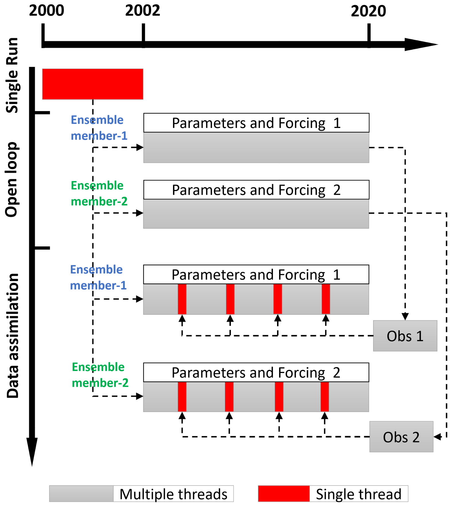
Figure 2 A schematic diagram to manage the threading pool of the DA workflow in PyGLDA, where an ensemble of two members for 2002–2020 is shown as an example.

3.3 GLDA configuration

3.3.1 Patch-wise domain localization

Running a high-resolution GHM with an ensemble-based DA system presents significant computational challenges, particularly when the ensemble size exceeds a few dozen members. Computational constraints and numerical stability issues become critical concerns, especially in large-scale Global Land Data Assimilation (GLDA) applications (Reichle and Koster, 2003). Given a limited ensemble size, spurious long-range correlations are easily introduced (Forman and Reichle, 2013; Khaki et al., 2017). These artificial correlations often degrade the DA performance by causing numerical instabilities during the Kalman update step, potentially leading to filter divergence. Consequently, compared to regional DA, traditional GLDA implementations face additional challenges related to computational feasibility and numerical robustness, making GLDA significantly more complex and less frequently attempted in previous studies.

To address these challenges, it is beneficial to restrict the spatial extent to which covariance matrices are computed. For global DA, it would be effective to divide the global domain into smaller localized patches. This technique, known as domain localization, helps stabilize the covariance matrix by assuming that significant correlations do not extend beyond a certain region. By enforcing this assumption, PyGLDA reduces the impact of spurious long-range correlations, improving numerical stability. Additionally, if both the hydrological model and GRACE-TWS observations exhibit only weak cross-domain correlations, DA computations within each patch can be treated as independent processes, making the GLDA problem computationally tractable. The assumption of independency is indeed too ideal but will be addressed in the next section. Therefore, in PyGLDA, the global domain is partitioned into patches (tiles), each operating as an independent DA unit. The patch size is flexible, but a recommended configuration for GRACE-based global DA is 18°×24°, as illustrated in Fig. 3. Each tile contains a set of grid cells, 3°×3°, which represent the smallest units used to aggregate GRACE observations. For future gravity missions with improved spatial resolution, such as MAGIC and NGGM (Daras et al., 2023), smaller grid sizes can be used accordingly.

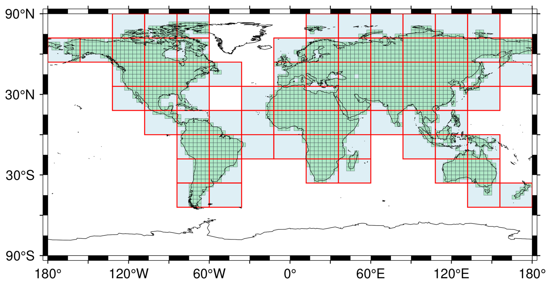
Figure 3 Configuration of the patch-wise domain localization, where each tile (denoted as the rectangle filled by the light blue) represents the “domain” to perform DA, individually. The unit box in black, contained in each tile, represents the smallest area to average GRACE observations to be assimilated.

Additionally, in PyGLDA, the domain size and configuration can be fully customized, allowing users to define different patch sizes depending on their specific application. The default setup excludes regions with no land coverage (such as oceans and ice sheets), leaving a total of 74 valid computational domains for DA (see Fig. 3). This flexible approach ensures that PyGLDA can be efficiently adapted to various spatial resolutions and study objectives. For example, users can modify the unit size (for example, using grid cells of 4 or 5°) or redefine domain boundaries based on a specific land mask. By employing this patch-wise DA strategy, PyGLDA effectively mitigates numerical instability issues and reduces computational costs, enabling high-resolution GLDA to be executed efficiently, even on standard computational platforms. Furthermore, this approach facilitates parallel computing, allowing multiple domain patches to be processed simultaneously, significantly accelerating GLDA execution.

3.3.2 Weighted global aggregation

In practice, the assumption of complete independence between adjacent domains (patches) is a simplification. Although it is reasonable to assume that correlations between the center of a patch and locations outside the patch are negligible – provided that the patch is sufficiently large – the same assumption does not hold for areas near the boundary of the patch (Reichle and Koster, 2003). Since PyGLDA performs DA independently within each patch, ignoring cross-boundary correlations can result in artificial discontinuities at the edges of neighboring patches. This issue, commonly referred to as the edge effect, manifests itself as visible artifacts in the global DA results, where abrupt transitions appear between adjacent patches. Therefore, to ensure smooth transitions across patch boundaries, PyGLDA introduces a weighted global aggregation strategy that effectively blends the DA results of neighboring patches.

To mitigate the edge effect, PyGLDA extends the computational domain of each patch by introducing overlapping regions with adjacent patches. These overlapping transition zones allow the DA results from neighboring patches to be smoothly blended, reducing artificial discontinuities. Specifically, each patch is extended by a predefined margin (for example 6° beyond its original boundaries, as shown in Fig. 4a), ensuring that DA calculations consider interactions between patch borders. After DA is performed within each extended patch, the overlapping regions are merged using a weighted averaging approach (see Fig. 4b and c). In this approach, each overlapping grid cell receives contributions from multiple patches, with weights assigned based on the distance from its outermost border. For example, $f^{\mathrm{a}}\left(x\right)=\sum _{i=\mathrm{1}}^{\mathrm{2}}{w}^i\left(\right|x-b^i\left|\right)f^i\left(x\right)$, where f^a denotes the averaged results of two patches (f¹ and f²), x denotes a certain point within the overlap area, bⁱ denotes the boundary of the patch ith, and w indicates the weighted function related to the distance $|x-b^i|$. The inverse distance weighting method used is based on the principle that correlations generally decay with increasing spatial separation (Reichle and Koster, 2003). The extension of 6° is considered based on our previous study on the length of GRACE's correlation (Yang et al., 2024a). This ensures a gradual transition between neighboring DA solutions, preserving spatial continuity.

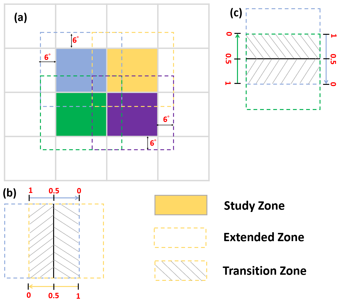
Figure 4 An illustration of the proposed global aggregation strategy. In (a), the box in grey replicates the tile/patch of Fig. 3. Four adjacent tiles (in blue/green/yellow/purple) are selected as examples to show the extension of the zone (in dashed line, e.g., 6°). A zoom-in is demonstrated in (b) and (c), where the shaded area indicates the overlap of two extended tiles, and the red number indicates the weight assigned to each tile for the averaging over the overlapping areas.

4 Application

4.1 Basin-scale DA for Danube

The Danube River Basin (DRB) is the second largest river basin in Europe, covering an area of approximately 801 463 km² and spanning 19 countries. Given its extensive transboundary nature, accurately monitoring terrestrial water storage changes within the DRB is crucial for water resource management, climate studies, and hydrological forecasting. To demonstrate the capability of PyGLDA in a regional DA context, we selected DRB as a case study. In this experiment, we performed basin-scale DA, a widely adopted approach in previous studies. However, in the next section, we extend this experiment to a grid-scale DA setup over the DRB to evaluate the added value of higher spatial resolution.

To implement the basin-scale DA, the boundaries of the Danube River Basin (DRB) and its sub-basins must be properly defined. Conventionally, the DRB is divided into three main subregions based on elevation and hydrological characteristics (Stagl and Hattermann, 2015): (1) the Upper Basin (UB), extending from the source of the Danube in Germany to Bratislava, Slovakia; (2) the Middle Basin (MB), the largest of the three subregions, stretching from Bratislava to the Iron Gate Gorge, a dammed section on the Serbia-Romania border; and (3) the Lower Basin (LB), covering the lowlands, plateaus and mountains of Romania and Bulgaria. Figure 5 illustrates the DRB and its sub-basin divisions, where the sub-basins serve as the smallest spatial units to average GRACE observations before assimilating into the model.

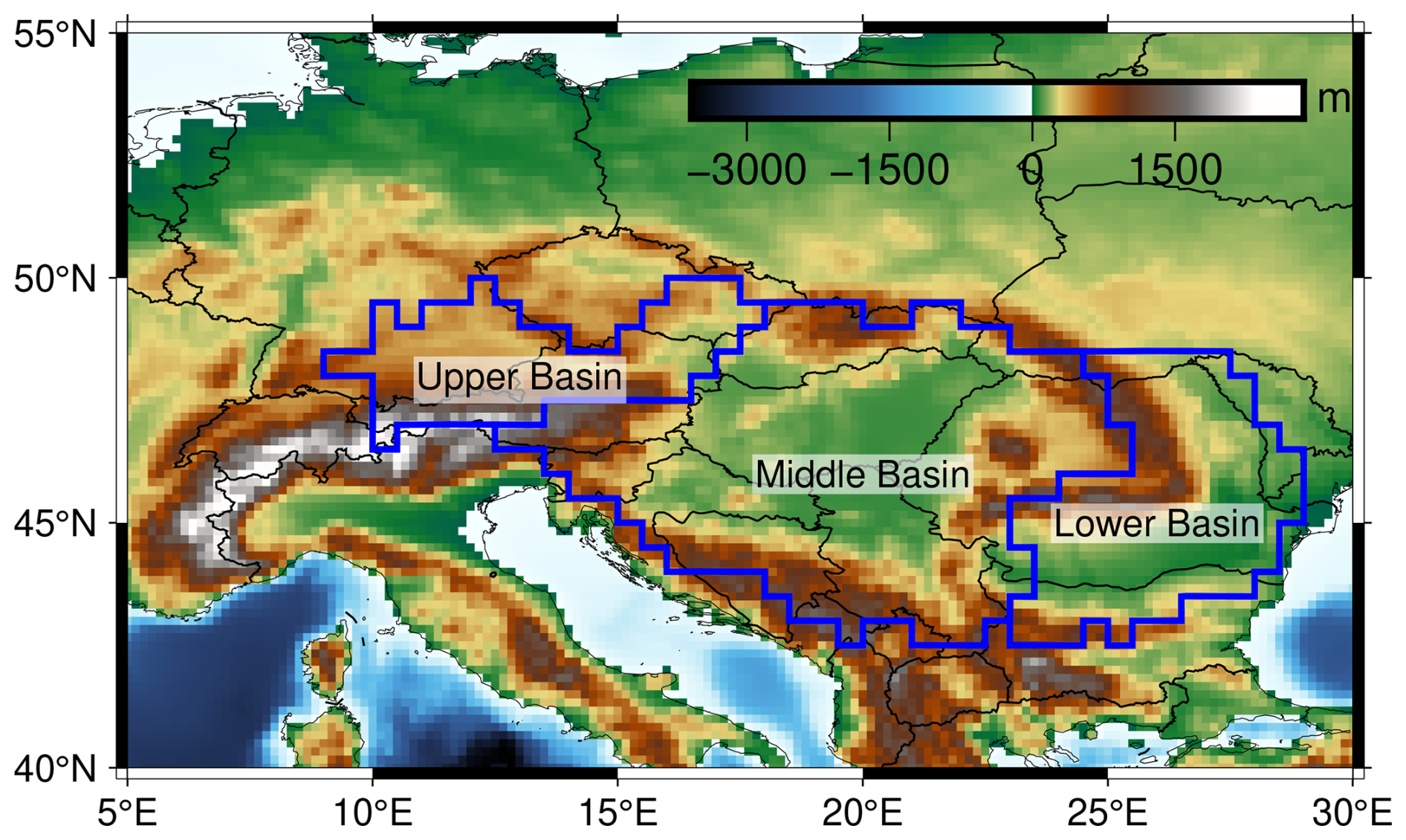
Figure 5 The Danube River Basin (DRB) and its three major subbasins. The basin's topography is shown as background picture.

The GRACE processing module is first executed to generate the observations required for assimilation. The specific GRACE processing configurations used in this study are summarized in Table 2. Then, the full propagation of covariance matrix from the harmonic domain to the gridded domain (that is, the basin-average TWS) is performed following the method of Yang et al. (2024a). Unlike many previous studies, which assume zero correlation between sub-basins, our analysis indicates that significant correlations exist, which cannot be ignored. For example, the correlation coefficient between UB and LB reaches 0.50 in January 2009, highlighting the importance of accounting for spatial correlations in DA. Furthermore, the temporal variability of the covariance structure is considered, since changes in the orbital height of the GRACE mission affect the error characteristics (Boergens et al., 2022).

Table 2 GRACE processing choice for the case study of DRB, see Table 1 for more details.

Previous studies suggest that an ensemble size of 30 provides a reasonable balance between computational efficiency and required data storage capacity on the one hand and representative error statistics on the other hand (Schumacher et al., 2018). It is also adopted for this case study. It is important to note that the number of MPI threads initialized must match the defined ensemble size; otherwise, an error will occur due to insufficient computational threads to handle all ensemble members. In this study, the ensemble members are generated by perturbing both the meteorological forcing fields and the model parameters. Specifically, random Monte Carlo sampling is applied using a triangular probability density function, introducing a multiplicative perturbation 30 % to these fields. The current version of PyGLDA assumes that perturbations are spatially correlated (homogeneous) but temporally uncorrelated (independently), although future versions will allow users to define arbitrary spatial-temporal correlation structures for generating perturbations.

Following the outlined strategy, we perform DA in the DRB for the period 2002–2010. Conventionally, the ensemble mean is considered the assimilated TWS estimate, while the ensemble spread serves as an approximation of uncertainty. However, the extent to which this spread of the ensemble accurately represents the true uncertainty remains an open question and requires further validation (Gerdener et al., 2023). Figure 6 illustrates the temporal variability of TWS and its major vertical components, providing insights into how DA redistributes the GRACE-based TWS increments across different water storage compartments. Among the five modeled components – surface water (Sr), topsoil water (S0), shallow soil water (Ss), deep soil water (Sd), and groundwater (Sg) – the largest DA-induced changes occur in groundwater and deep soil water, while surface and topsoil water capture mainly high frequency variations from GRACE. This finding is consistent with previous studies that indicate that GRACE-based TWS anomalies primarily constrain slow-varying subsurface water storage components rather than short-term surface fluxes.

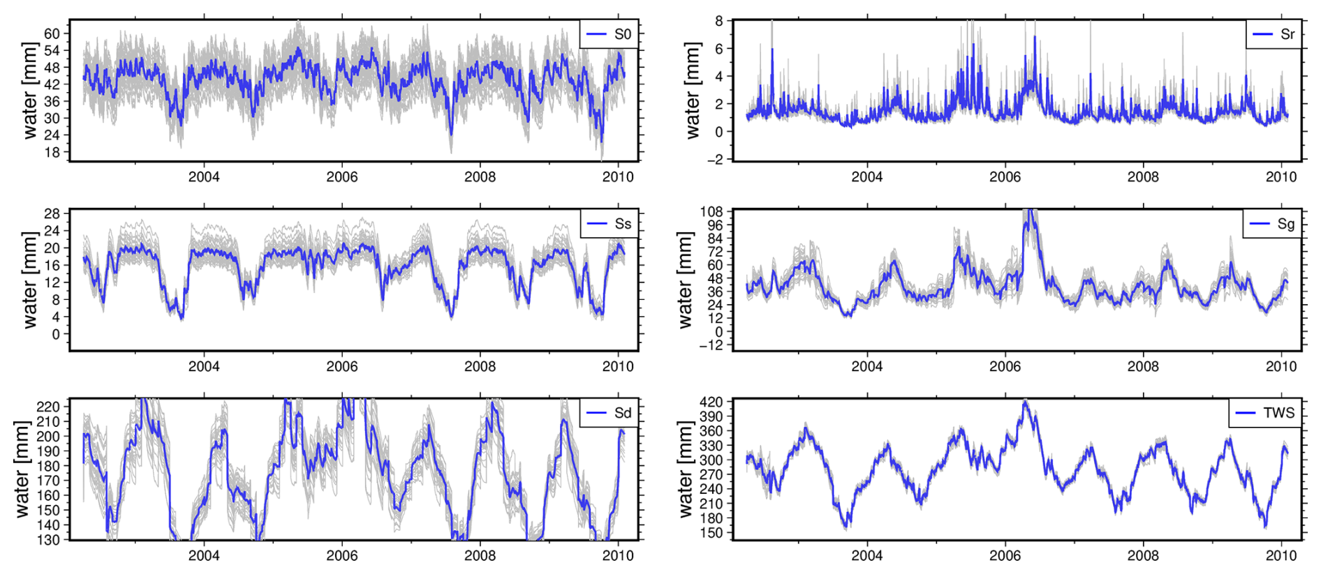
Figure 6 An overview of the mean (in blue) of the ensemble (shaded) estimates after Basin-scale DA experiment over DRB is illustrated. Plots include the TWS estimate and its major vertical compartments: surface water (Sr), topsoil water (S0), shallow soil water (Ss), deep soil water (Sd), and groundwater (Sg).

Furthermore, Fig. 7 presents the basin-averaged TWS time series for the entire DRB and its three sub-basins (UB, MB, and LB), comparing the results from the open-loop (OL) simulation, the DA run, and GRACE observations. A comparison between GRACE (black dots) and OL (shaded line) reveals that while the model preserves more short-term dynamics, GRACE exhibits larger magnitude variations, highlighting the need for DA to optimally merge both sources of information. As expected, the DA result (green line) adjusts the magnitude of the TWS closer to GRACE while retaining the temporal variability of the model. In particular, in Fig. 7b, an evident phase shift exists between OL and GRACE, probably due to a delay in the streamflow response. For example, across the entire DRB, the annual signal phase for OL, GRACE, and DA is found to be −41, 29, and 11°. Therefore, the DA process successfully reduces this phase mismatch, although further validation is required using in situ observations to confirm the accuracy of this correction.

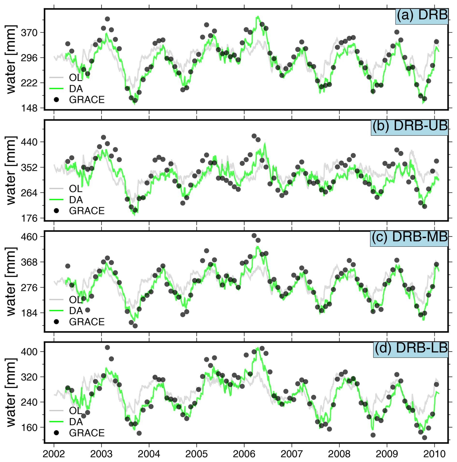
Figure 7 An overview of the basin averaged TWS of DRB and its three sub-basins (LB, MB, and UB) for OL, DA and GRACE observations.

To further analyze the spatial characteristics of the assimilation results, we extract the long-term trend and seasonal amplitude of the TWS estimates based on OL, DA and GRACE and present them as 2D spatial maps in Figs. 8 and 9. The original spatial resolution of the OL and DA outputs is 0.1°, but for comparison with GRACE, an up-scaling procedure is applied, aggregating the data to the resolution 0.5°. Furthermore, a 2D spline smoothing technique is applied to improve visualization clarity, as shown in Figs. 8d–f and 9d–f. The trend analysis in Fig. 8 reveals that while DA largely preserves the spatial pattern of the OL model, it brings the upper Danube Basin (UB) trends closer to the GRACE observations. Quantitative comparisons indicate a spatial correlation of 0.74, 0.98, and 0.89 between DA and OL in the UB, MB, and LB sub-basins, respectively. However, the correlation between DA and GRACE is lower (0.79, 0.35, and 0.75), particularly in the MB region, suggesting that DA is more dependent on the model when the discrepancies between GRACE and the model are large. Likewise, by looking at the annual amplitude in Fig, 9, one can see that DA perfectly replicates the spatial pattern of OL, with a spatial correlation coefficient up to 0.92; but meanwhile, its spatial magnitude has been tuned much (almost twice larger than OL) toward GRACE observations. In this sense, PyGLDA has fulfilled its goal of balancing the model and observations to reach the statistically optimal combination.

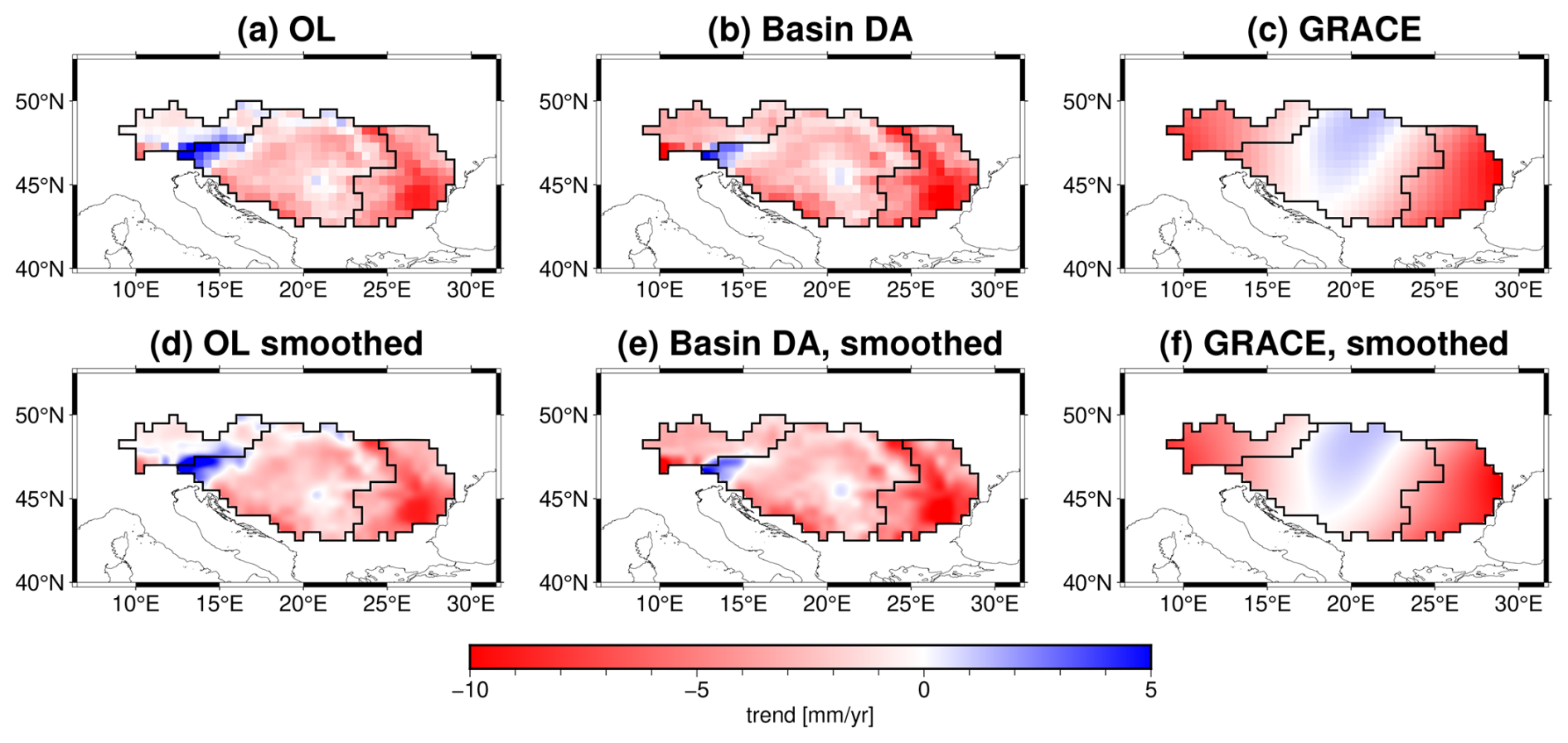
Figure 8 The secular trend of TWS over 2002–2010 for DRB, where the OL, DA and GRACE results are listed at (a)–(c), and a smoothed version is respectively shown at (d)–(f) for a better visualization.

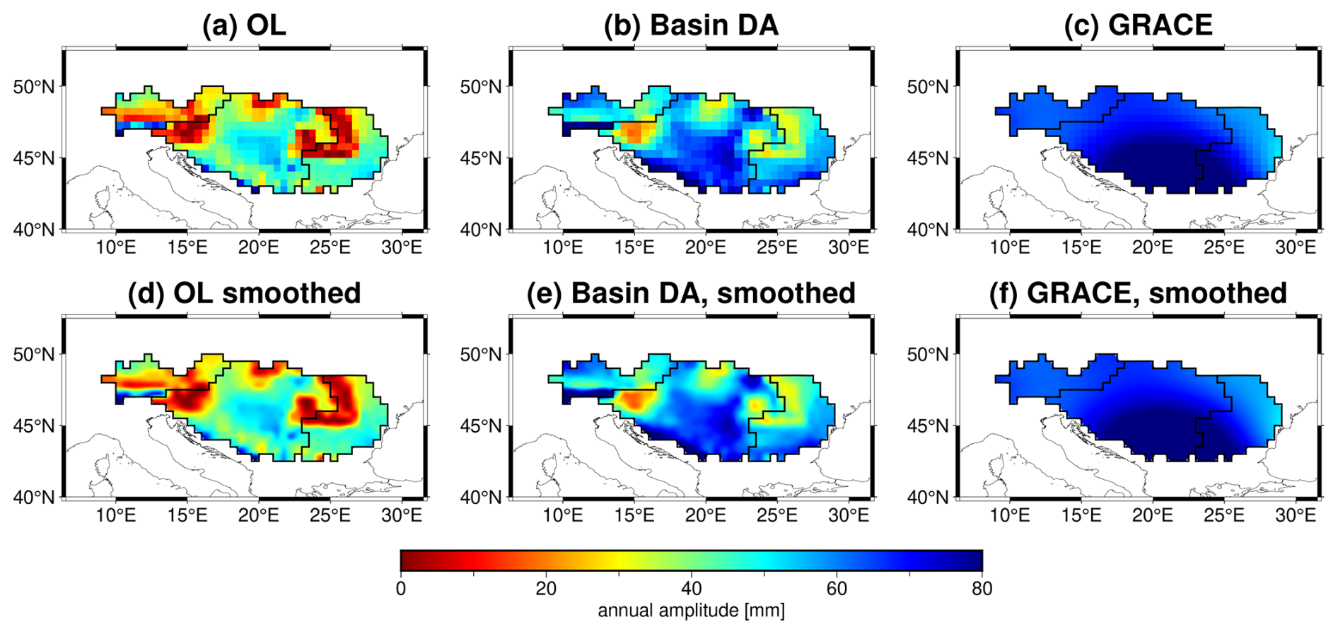
Figure 9 An overview of the annual amplitude of TWS within DRB over 2002–2010, where the OL, DA and GRACE results are shown in (a)–(c), and a smoothed version is respectively shown at (d)–(f) for a better visualization.

4.2 Grid-scale DA within DRB

In recent years, there has been a growing interest in DA on a grid scale using GRACE gridded data products, such as the 3°×3° mascon solutions from JPL. Thus, we have added this possibility to PyGLDA to accept Mascon solutions directly, for example, the CSR mascon solutions (Save et al., 2016) are integrated in this study. Compared to basin-scale DA, grid-scale DA allows for a finer spatial representation of GRACE-TWS signals, potentially improving the assimilation of satellite gravity data into high-resolution hydrological models (Girotto et al., 2016; Khaki et al., 2017; Li et al., 2019; Gerdener et al., 2023). In this section, we extend our previous basin-scale DA experiment over the DRB by implementing a grid-scale DA approach. It is important to note that PyGLDA does not require structural modifications or particular operations to perform grid-scale DA; users simply need to define the target region using a shapefile, regardless of whether the intended DA is at the basin or grid scale. For a grid-scale DA, the shapefile defines each grid cell as the sub-basin. This feature highlights the flexibility of PyGLDA, which allows seamless transitions between different spatial scales.

For this experiment, we adopt a widely used grid resolution of 3°×3° for GRACE observations, ensuring consistency with previous grid-scale DA studies. The grid cells are defined to fully cover the DRB, as illustrated in Fig. 10, where each numbered cell represents an individual assimilation unit. However, be aware that a uniform grid structure cannot be ensured, and one can see from Fig. 10 that some cells are irregular in shape (for example, cell 7), with their boundaries intersecting the edges of the basin. In total, the DRB is divided into 19 computational cells, each serving as an independent observation region for GRACE-TWS averaging and assimilation. Although the irregularity of some cells does not significantly affect the assimilation process, optimizing the grid generation approach for basins with complex geometries remains a potential area for future improvement.

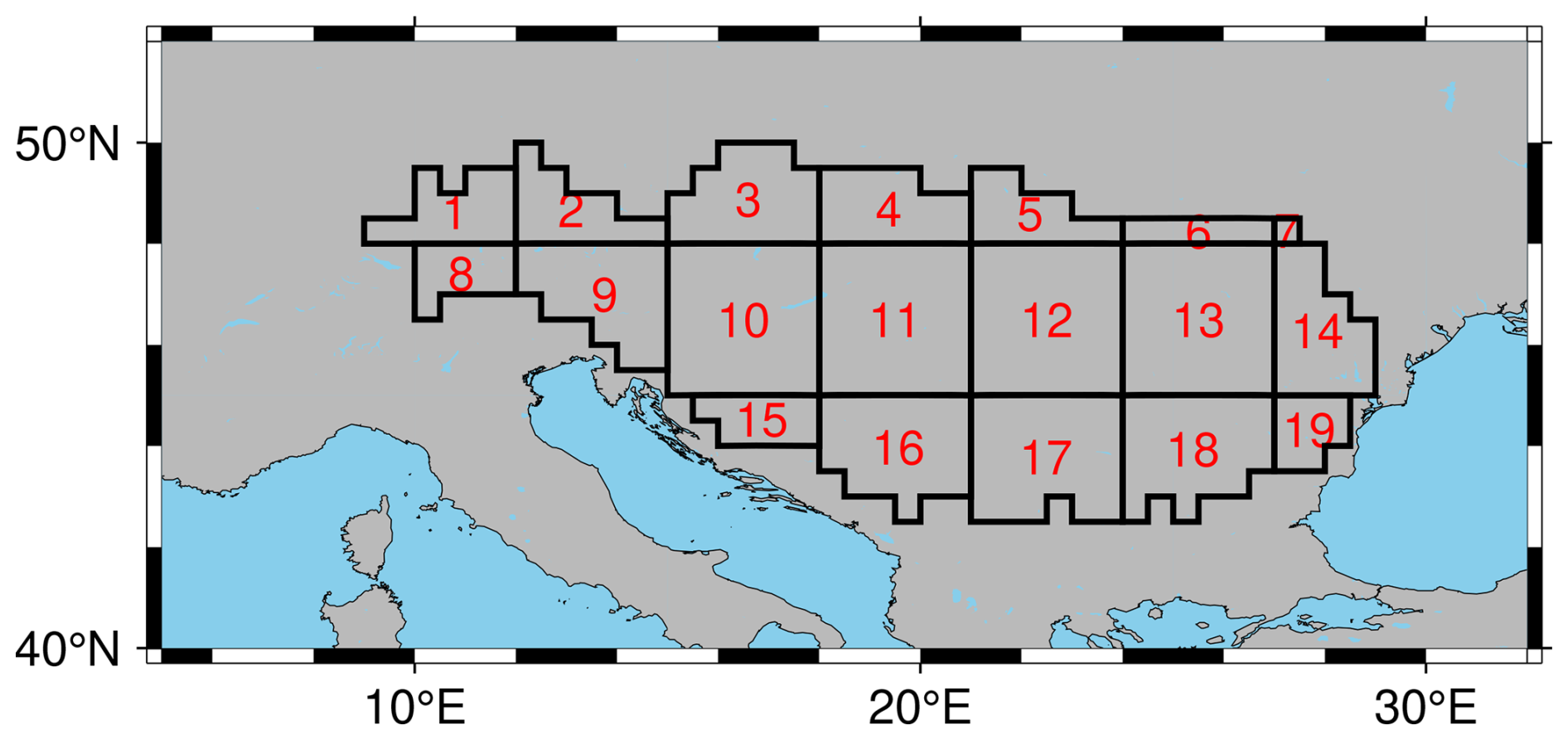
Figure 10 An overview of the 3°×3° cell definition for DRB, where the identification number (ID) of each cell is highlighted in red.

Following the grid definition in Fig. 10, we calculate GRACE-TWS anomalies for each 3°×3° cell by averaging the original 0.5° gridded GRACE data within the limits of each cell. In addition, we investigated the spatial correlation structure of GRACE observations in these grid cells, as shown in Fig. 11. The results reveal that strong spatial correlations exist between many grid cells, with some correlation coefficients exceeding 0.9. Additionally, evident negative correlations appear, likely due to residual correlated noise from imperfect GRACE decorrelation filtering. These findings suggest that assuming uncorrelated observation errors, as done in some traditional DA implementations, may not be entirely realistic. Instead, PyGLDA explicitly incorporates the full covariance matrix of GRACE observations, ensuring that spatial correlations are properly accounted for during the assimilation process.

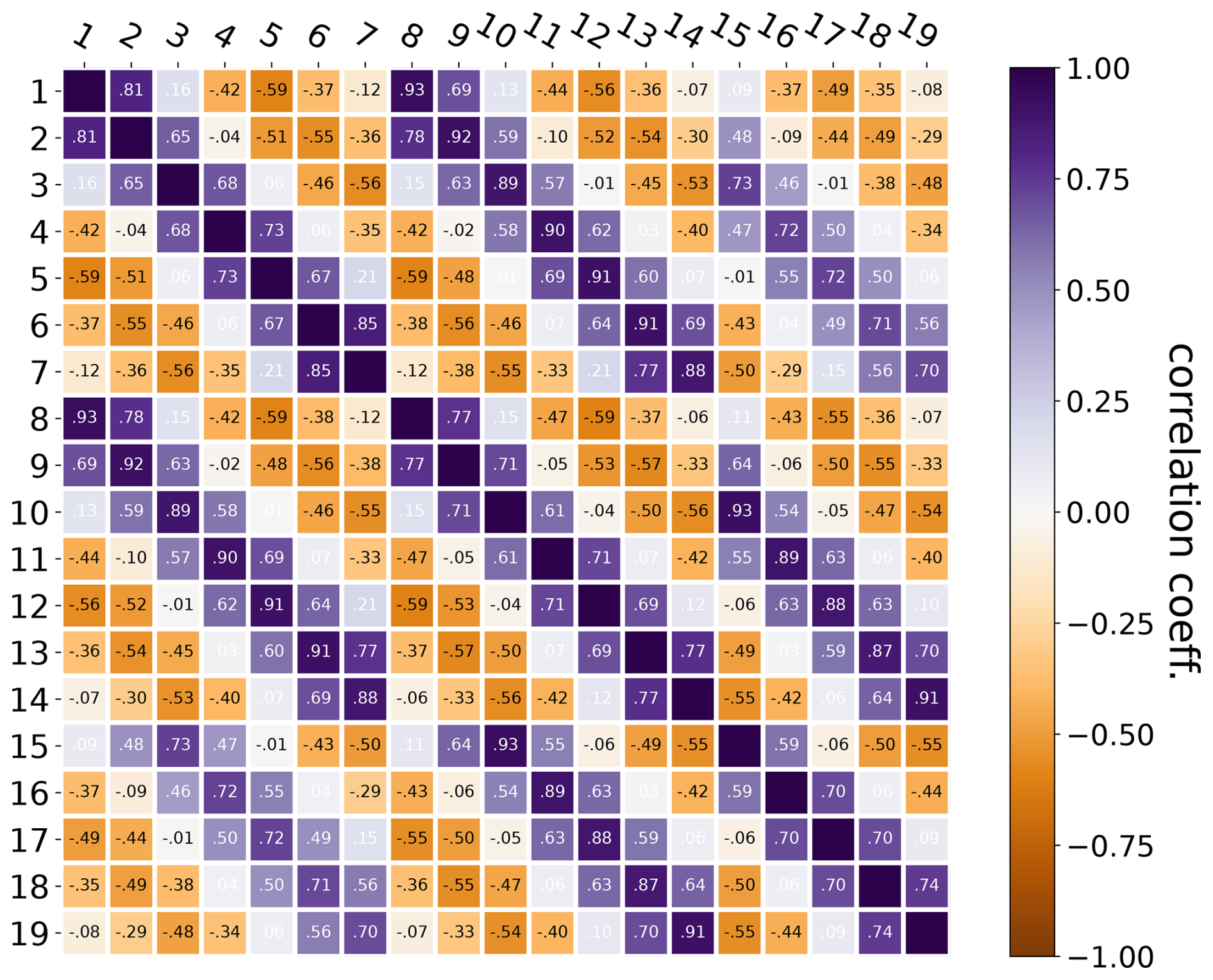
Figure 11 Spatial correlation coefficients of GRACE observations for cells within DRB. The label of X(Y) axis denotes the cell ID as indicated by Fig. 10.

Keeping the GRACE processing and perturbation (including model) strategies unchanged from the basin-scale DA experiment, we now perform grid-scale DA over the DRB using PyGLDA. The ensemble-averaged results are presented in Fig. 12, where, for brevity, only the basin-averaged TWS (rather than the individual compartment) is shown. A comparison between grid-scale DA (Fig. 12) and basin-scale DA (Fig. 7a) indicates that at the basin-wide scale, the two assimilation strategies produce generally similar results. The temporal correlation between the basin-averaged TWS estimates from the two DA approaches is found to be 0.99, suggesting that, at large spatial scales, grid-scale DA does not significantly alter basin-wide statistics. However, this does not diminish the importance of grid-scale DA, as its primary advantage likely lies in capturing finer spatial details, which are further explored in the subsequent 2D spatial analysis. Furthermore, the consistency between basin-scale and grid-scale DA results confirms the correctness and robustness of PyGLDA’s grid-scale DA implementation.

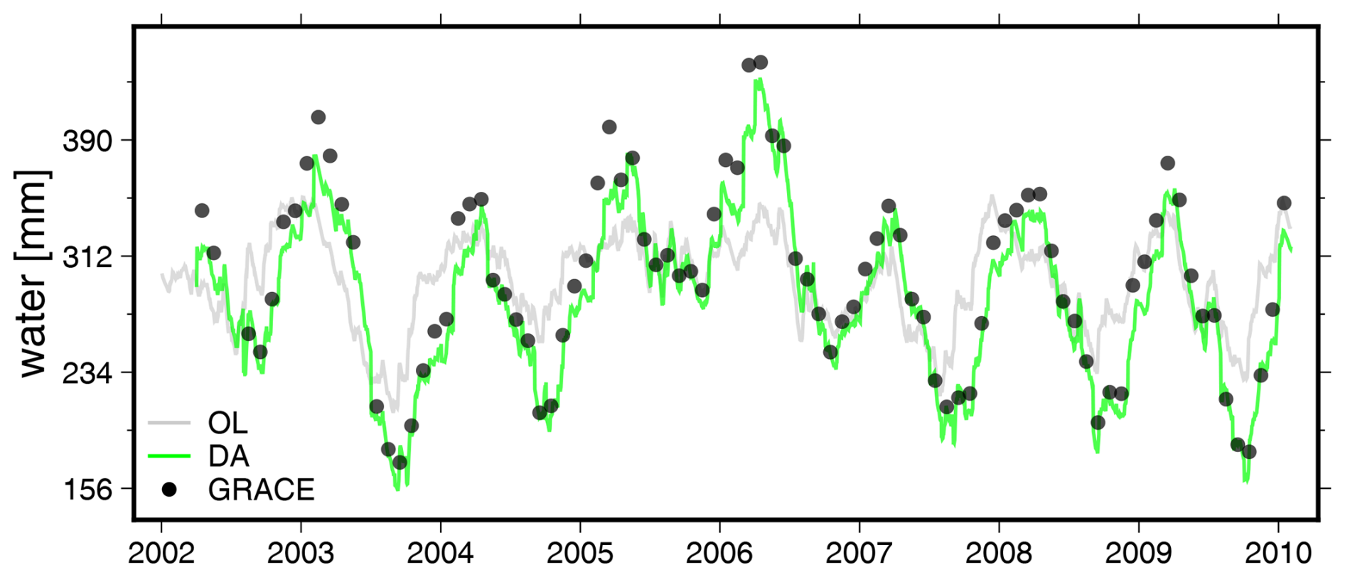
Figure 12 An overview of the basin averaged TWS of DRB for OL, grid-scale DA and from GRACE observations.

To further examine the spatial characteristics of grid-scale DA, we compare the long-term trends and seasonal amplitudes of the OL, DA, and GRACE-TWS estimates at a resolution of 0.5°, as shown in Figs. 13 and 14. Comparing the DA trend maps in Fig. 13e (grid-scale DA) and Fig. 8e (basin-scale DA), we observe that grid-scale DA more closely follows GRACE-TWS trends, particularly in the Middle Basin (MB). For example, the positive trend signal (indicating a water gain) found in the heart of MB (∼20° E, ∼45° N) appears more evident in Fig. 13e than in Fig. 8e, and such a positive signal is quite consistent with that of GRACE-TWS. Similarly, in Fig. 14, we see that DA on the grid scale better captures the magnitude of the annual amplitude variations observed in GRACE, reducing the Root Mean Squared of Differences (RMSD) between GRACE and DA from 22.1 mm (basin scale) to 16.5 mm (grid scale). Furthermore, the spatial correlation between DA and GRACE improves from 0.45 (basin scale) to 0.51 (grid scale), further demonstrating the added value of grid-scale DA in preserving finer-scale spatial information. These findings suggest that incorporating higher-resolution GRACE-TWS observations into the DA process allows a better spatial representation of water storage changes, particularly in regions where the hydrological model and observations exhibit significant differences. By integrating finer-scale satellite-derived TWS anomalies, grid-scale DA provides a more detailed and accurate spatial distribution of water storage variability compared to basin-scale DA. This is particularly relevant for future satellite gravity missions, such as MAGIC and NGGM (Daras et al., 2023), which are expected to offer higher spatial and temporal resolution with improved error characteristics (Daras et al., 2023). However, while these results highlight the advantages of grid-scale DA, it is important to note that neither approach can be universally considered superior. The optimal choice between basin-scale and grid-scale DA depends on factors such as study objectives, model resolution, and observation uncertainties. Future research should include independent validation using in situ measurements, such as groundwater well data and river discharge records, to further assess the accuracy of these DA strategies.

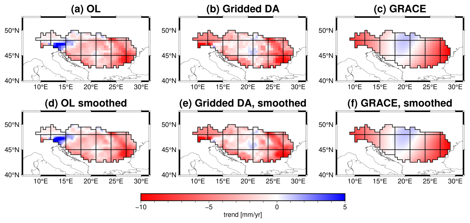
Figure 13 As that of Fig. 8 but this is for the grid-scale DA.

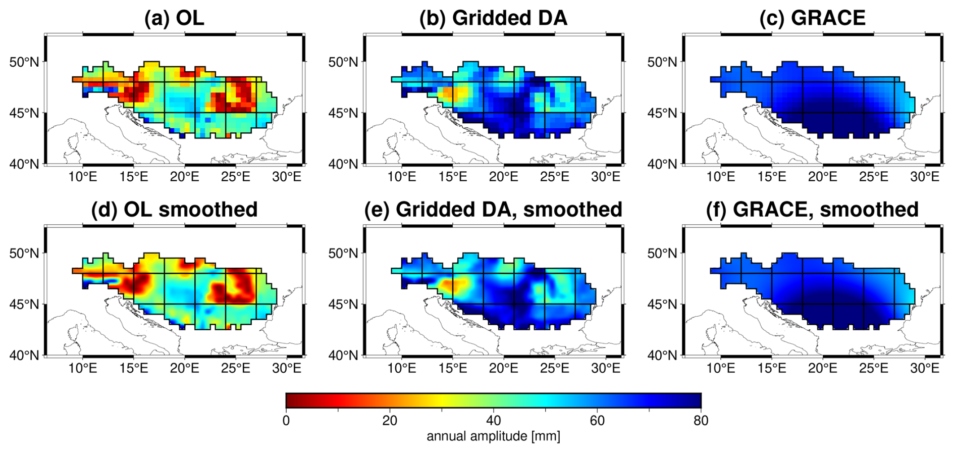
Figure 14 As that of Fig. 9 but this is for the grid-scale DA.

4.3 0.1° and daily GLDA

In this case study, we performed the GLDA experiment covering 2002–2010 by merging monthly GRACE TWS into daily W3RA globally at high spatial resolution, that is, 0.1° or equivalently 10–12 km, which is likely the highest resolution among similar previous efforts. Here, we follow the patch-wise domain localization and weighted global aggregation as described in Sect. 3.3 to ensure numerical stability and avoid artificial discontinuities in the DA results. The overall implementation of GLDA is conceptually illustrated in Fig. 15, where one can see the global distribution of the patches (red rectangles): the shape of the “basin” inside each patch (in blue) and the “sub-basins” inside each “basin” (black boxes). The global domain is divided into 74 computational patches, each spanning 18°×24°, with overlapping regions (extended by 6°) incorporated to ensure smooth transitions across patch boundaries (see Fig. 15). Greenland and Antarctica are excluded because GHMs often do not cover these regions. All the shapefiles related to the aforementioned definitions are shared in the PyGLDA package. The DA is performed independently for each patch, followed by a weighted global aggregation step to merge neighboring DA solutions.

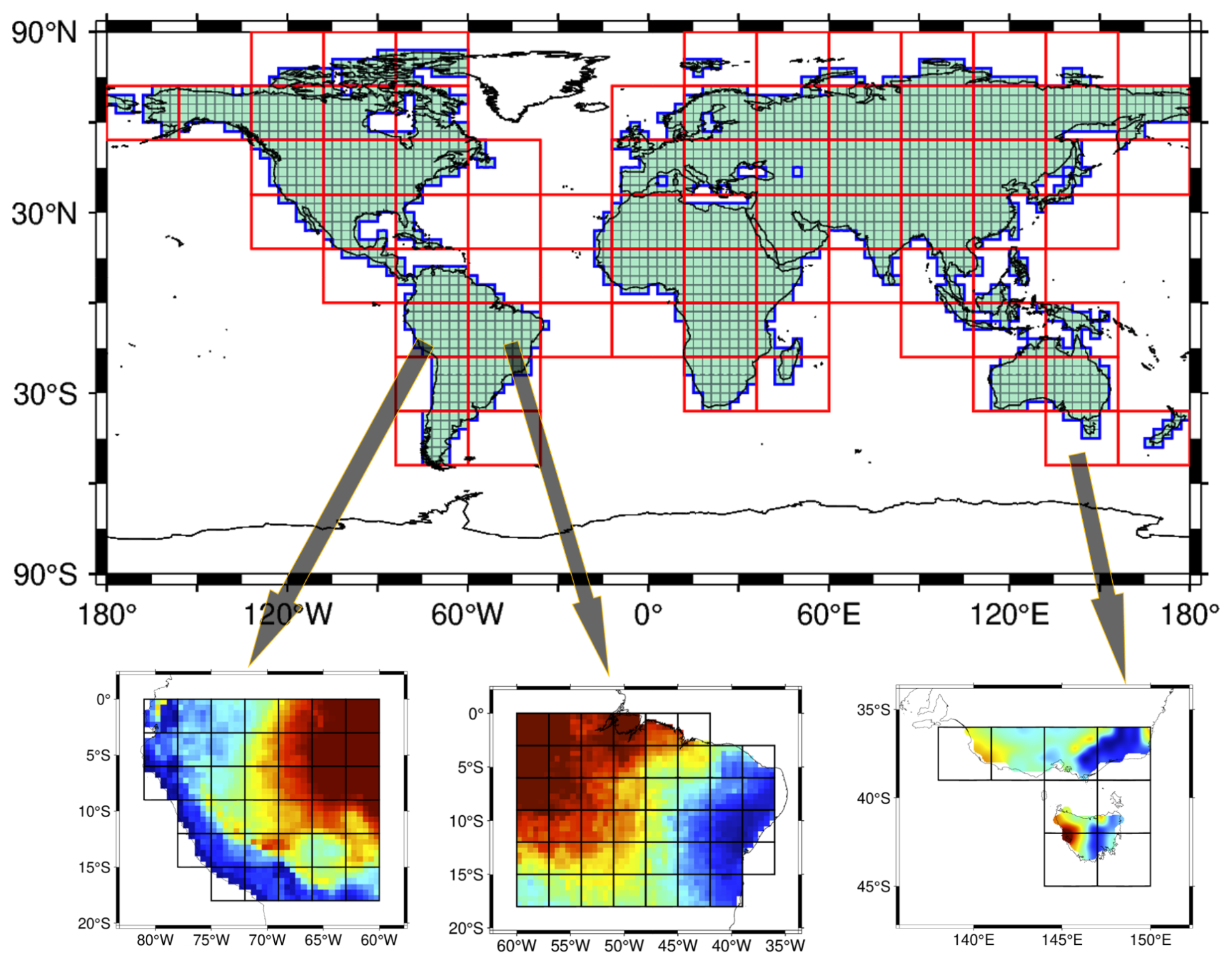
Figure 15 A schematic diagram of the GLDA implementation, where extension of the zone (6° as indicated by Fig. 4) has been applied but not shown here for simplifying the visualization.

Furthermore, the detailed execution of global DA (GLDA) in our implementation is outlined in Table 3, summarizing how each sub-module of PyGLDA is utilized and how efficient it is for specific tasks. The workflow is divided into three main stages: (1) data pre-processing, (2) data processing, and (3) data post-processing, each comprising multiple sub-steps. This structured approach facilitates performance evaluation and optimization of computational efficiency. We conducted the GLDA tests on an in-house computing cluster, using a single node equipped with 32 cores (Intel Xeon Gold 613 @1.59 GHz) and 192 GB of RAM. While computational demands vary based on the user's specific setup, our test results provide a baseline reference for PyGLDA's efficiency. From Table 3, our tests indicate that data preparation is the most time consuming, followed by data processing and post-processing. Fortunately, the data preparation only requires to be run once and the results can be saved for repeat use in later stages. In addition, currently the running time is tested for data preparation based on a single thread, which means that a considerable reduction of computation time could be expected through multi-thread parallelization in future update. In contrast, the data processing (responsible for DA) as the core of the GLDA, is super fast and should be affordable even on a personal desktop. For example, the total time it takes to run data processing for a regional DA in DRB (as indicated in Sect. 4.2) is less than 15 min on our platform. For the GLDA in this section, the total time for running the global DA experiment is approximately 5 d at the single node of the cluster, but be aware that more than half of the time goes to the data preparation. Then, one can expect a higher efficiency by making use of multiple nodes. Despite the satisfactory efficiency, PyGLDA has a high demand of the data storage for GLDA. In this case study, the amount of temporary files and output overall has already been up to 15 TB, due to the high temporal (daily), horizontal (0.1°, i.e., 2 142 930 grid points), and vertical (eight layers) resolution at global scale.

Table 3 An overview of the numerical efficiency tests for PyGLDA, where the computation is designed from years 2002–2010 with an ensemble size of 30.

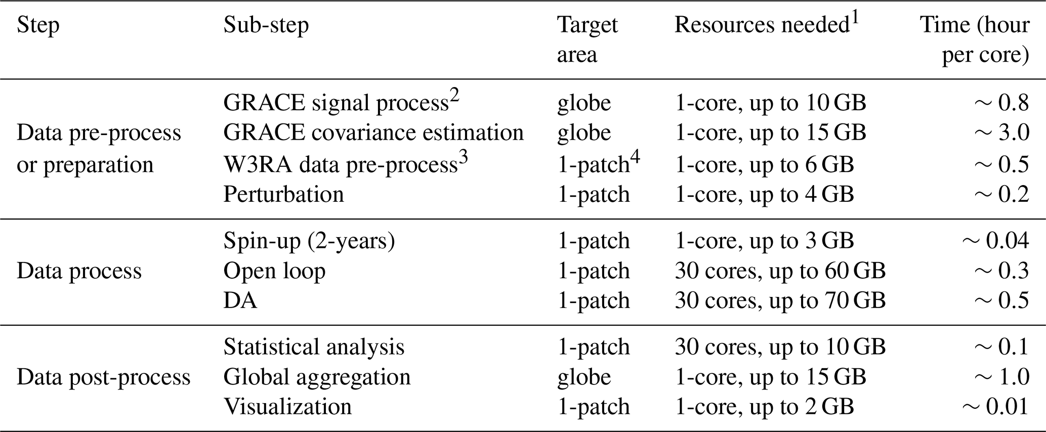
¹ CPU cores and running memory for serial/parallel computations. ² This includes conversion from GRACE Level-2 to TWS and necessary corrections as indicated by Table 2. ³ This includes the crop of ERA5-land forcing field (as well as the model parameters and climatology) at intended area, and its upscaling to a desired resolution. ⁴ This indicates the performance is evaluated on one patch as defined in Fig. 15.

Then, the TWS results (from the model, GRACE observation, and GLDA) are collected in Fig. 16. By comparing the trend map between W3RA and GRACE, one can see a very evident underestimation of the trend in TWS on a global scale in the model, which was also confirmed by previous studies that current models cannot well reproduce long-term change, particularly in groundwater (Scanlon et al., 2018; Mehrnegar et al., 2020; Forootan et al., 2024), and other evidence that shows groundwater is declining worldwide (Jasechko et al., 2024). GRACE TWS shows larger trends, but its spatial resolution is too coarse for hydrological interpretation. In short, the model is poor at revealing the magnitude of trends, but can benefit from a high spatial resolution. Fortunately, GLDA can use these two features in a complementary way, where, for example, in Fig. 16, one can see that DA results adopt the resolution of W3RA and the trend magnitudes are successfully tuned to GRACE. In statistics, as for the trend map, the spatial correlation between W3RA and DA is found to be 0.12, which is because the original model does not represent trends well. The correlation between GRACE and DA is increased to 0.35. The global mean (latitude weighted) RMS (Root Mean Squared) of the differences between W3RA and DA is found to be 50.0 mm yr⁻¹, while that of GRACE and DA is 45.1 mm yr⁻¹. Regarding the annual amplitude, the spatial correlation between W3RA and DA is found to be 0.86, while that between GRACE and DA is 0.92; the global mean RMS of differences between W3RA and DA is 26.0 mm, whereas that between GRACE and DA is 29.0 mm. Based on these results, it seems that the DA is more dependent on GRACE than on the W3RA model, in terms of trend and seasonality. Nevertheless, the current experiment might not be optimal, since the weight of the model also depends on how the ensemble is generated, and proper tuning of the model covariance should be subject to more investigation. In addition, validations of the proposed GLDA against independent data sets are desirable, which will be addressed in our future release of the GLDA product.

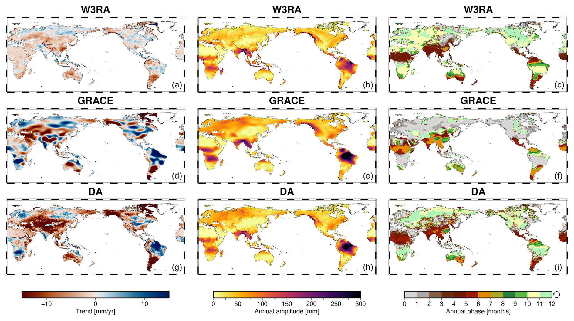
Figure 16 TWS results (2002–2010) in terms of secular trend (a, d, g), annual amplitude (b, e, h) and annual phase (c, f, i). Plots from the top to the bottom correspond to W3RA (open-loop ensemble-mean model output), GRACE (perturbation-free observations), and the assimilated results. For appropriate visual comparison, the results of W3RA and DA are upscaled from 0.1 to 0.5° to be consistent with GRACE-TWS. The annual phase is defined as the month of year when TWS reaches its maximum.

5 Limitations

PyGLDA consists of three main modules: (1) GHM, (2) GRACE observations, and (3) the DA system. Consequently, each of these modules introduces potential limitations that can affect the performance of PyGLDA, and they should be individually addressed. However, the limitations listed below are not exhaustive but represent the most critical challenges that should be prioritized in future updates.

• GHM: (1) the W3RA model does not account for anthropogenic water use, such as irrigation, which significantly affects the global water cycle. For example, in regions such as the north China plain, excessive groundwater extraction for irrigation is a major contributor to water depletion, but it is not well represented in W3RA. Consequently, model estimates in these regions may be less reliable. (2) Although W3RA includes a snow module, it does not adequately capture water storage changes in glaciated regions. For example, GRACE detects a strong ice-melting signal over Alaska, which is poorly represented in W3RA, leading to less accurate vertical disaggregation of water storage in glacier-covered areas.

• GRACE: (1) spatial leakage remains a significant limitation. Although PyGLDA excludes lake storage, the inherent spatial leakage of satellite gravity data can introduce artificial signals into adjacent areas, affecting the DA results in regions with significant changes in lake water, such as areas near the Caspian Sea. (2) Uncertainty in the true spatial resolution of GRACE. Larger grid cells improve the signal-to-noise ratio, but result in a loss of spatial detail. Although PyGLDA allows users to flexibly define the grid size for GRACE observations, determining the optimal balance between spatial resolution and noise remains an open question.

• DA: (1) the current perturbation module in PyGLDA is sub-optimal for both forcing fields and model parameters. The current implementation assumes spatial homogeneity in perturbations to prevent spatially independent perturbations from canceling out at the basin scale. However, this simplification may lead to unrealistic model uncertainty representations, ultimately degrading DA performance. Future improvements should explore spatially correlated perturbation strategies to enhance covariance realism. (2) Covariance localization is currently absent. Although no clear signs of filter divergence have been observed in PyGLDA due to its patch-wise and coarse grid implementation (e.g., 3° grid cells), users may face potential risks of filter divergence when using finer grid configurations, such as 1° resolution. Incorporating traditional covariance localization techniques, such as the Schur product method (Webber and Morzfeld, 2023), could improve the stability and robustness of PyGLDA in future updates.

6 Conclusions

This study introduces PyGLDA, a community-level and open-source high-resolution global land data assimilation (DA) system designed to integrate GRACE/GRACE-FO-derived TWS observations with global hydrological models (GHMs). Our major contribution is that PyGLDA can be used globally and regionally at various resolutions over arbitrary regions of the land. In addition, PyGLDA can allow users to flexibly switch between grid- and basin-scale DA. Unlike previous global DA implementations, PyGLDA features a patch-wise domain localization strategy and a weighted global aggregation scheme, which enhance computational efficiency and ensure smooth spatial transitions across assimilation regions. Our results demonstrate that PyGLDA effectively reduces discrepancies between model-based TWS estimates and GRACE observations, providing an improved representation of long-term trends and seasonal water storage variations at global and regional scales.

Beyond its current capabilities, PyGLDA provides a flexible and scalable DA framework that can be extended for multi-sensor hydrological data assimilation. Future developments will focus on incorporating additional observational datasets, such as satellite-based soil moisture retrievals, to further improve the reliability of water storage estimates. Additionally, advances in satellite gravimetry, including upcoming missions like MAGIC and NGGM, may offer higher spatial and temporal resolution with improved error characteristics, enabling even more precise DA applications. The modular nature of PyGLDA ensures that it can seamlessly integrate with these future sensor datasets, making it a valuable tool for hydrological modeling, climate studies, and water resource management.

Furthermore, although PyGLDA is designed for multi-GHM compatibility, this study focuses primarily on W3RA. In future updates, a more advanced GHM such as WaterGAP 2.2e (Müller Schmied et al., 2024), could be considered an effective alternative to account for the use of anthropogenic water, reservoirs, lakes, and glaciers. Other promising and feasible extensions may include (i) adding covariance localization to stabilize the filter, (ii) accounting for reasonable spatio-temporal perturbation (e.g., with local correlation) to better simulate the model covariance, and (iii) simulating lake signal and reducing its spatial leakage from GRACE-TWS observations (Deggim et al., 2021).

Appendix A: EnKF and EnKS

The Ensemble Kalman Filter (EnKF) is a merger that applies observations to update the state and parameters of the model based on their relative errors (Evensen et al., 2009). Model errors are generated by a Monte Carlo simulation that considers n ensemble members of the model parameters (Θ_i) expressed as:

$$\begin{array}{}\text{(A1)}& {\mathbf{\Theta }}_i={\mathbf{\Theta }}_{\mathrm{0}}+{\mathit{\xi }}_i,i=\mathrm{1},\mathrm{\dots }n,\end{array}$$

where ${\mathbf{\Theta }}_{{\mathrm{0}}_{m\times \mathrm{1}}}$ (m being the number of parameters) is a vector representing the initial values of the model parameters. Random errors (ξ_i) are introduced to perturb the initial values of the ‌parameters. The distribution of these errors can be Gaussian and triangle (Schumacher, 2016). In our study, nine model parameters are selected to be perturbed, thus m=9. In addition to the parameters, the forcing fields are perturbed as well following

$$\begin{array}{}\text{(A2)}& {\mathit{M}}_i={\mathit{M}}_{\mathrm{0}}+r_i,i=\mathrm{1},..\mathrm{\dots }n,\end{array}$$

where ${\mathit{M}}_{{\mathrm{0}}_{p\times q}}$ (p being the number of grid points, q being the number of forcing fields) is a vector representing the initial values of the forcing inputs. Random errors (r_i) are considered to perturb the initial values of these errors. In PyGLDA, for example, we consider multiplicative errors for precipitation, temperature, and short-wave solar radiation, thus q=3. The forecast model state (denoted by the upper index “f”) of an ensemble member is then produced by

$$\begin{array}{}\text{(A3)}& {\mathit{x}}_i^{\mathrm{f}}=F\left({\mathbf{\Theta }}_i,{\mathit{M}}_i\right),i=\mathrm{1},\mathrm{\dots }n,\end{array}$$

where x indicates the model state and x^f is the forecast state. For example, we adopt n=30 ensemble members to perform our experiments of Sect. 4. As a result, these 30 members constitute an ensemble, i.e., ${\mathbf{X}}_{p\times n}^{\mathrm{f}}$, following

$$\begin{array}{}\text{(A4)}& {\mathbf{X}}^{\mathrm{f}}=\left({\mathit{x}}_{\mathrm{1}}^{\mathrm{f}},\mathrm{\cdots },{\mathit{x}}_n^{\mathrm{f}}\right),\end{array}$$

from which the ensemble mean of the forecast states is obtained by

$$\begin{array}{}\text{(A5)}& {\stackrel{\mathrm{‾}}{\mathit{x}}}^{\mathrm{f}}={\displaystyle \frac{\mathrm{1}}{n}}\sum _{i=\mathrm{1}}^n{\mathit{x}}_i^{\mathrm{f}},\end{array}$$

with the error covariance matrix (${\mathbf{C}}_{p\times p}^{\mathrm{f}}$) of the forecast states:

$$\begin{array}{}\text{(A6)}& {\mathbf{C}}^{\mathrm{f}}={\displaystyle \frac{\mathrm{1}}{n-\mathrm{1}}}\sum _{i=\mathrm{1}}^n\left({\mathit{x}}_i^{\mathrm{f}}-{\stackrel{\mathrm{‾}}{\mathit{x}}}^{\mathrm{f}}\right){\left({\mathit{x}}_i^{\mathrm{f}}-{\stackrel{\mathrm{‾}}{\mathit{x}}}^{\mathrm{f}}\right)}^T.\end{array}$$

The analysis step (shown by the upper index “a”) corrects the forecast states and their covariance matrix using the GRACE-TWS observations, which yields

$$\begin{array}{}\text{(A7)}& {\displaystyle }& {\displaystyle }{\mathbf{X}}^{\mathrm{a}}=\left({\mathit{x}}_{\mathrm{1}}^{\mathrm{a}},\mathrm{\cdots },{\mathit{x}}_n^{\mathrm{a}}\right)={\mathbf{X}}^{\mathrm{f}}+\mathbf{K}\left(\mathbf{Y}-{\mathbf{HX}}^{\mathrm{f}}\right),\text{(A8)}& {\displaystyle }& {\displaystyle }{\mathbf{C}}^{\mathrm{a}}=(\mathbf{I}-\mathbf{KH}){\mathbf{C}}^{\mathrm{f}},\end{array}$$

where Y_p×n is an ensemble of GRACE-TWS observations, which is produced from the covariance matrix of observations (Yang et al., 2024a). For the example of Sect. 4.2, the dimension of Y is 19×30, and for the global GLDA (Sect. 4.3) with grid resolution 3°, the dimension is roughly 1700×30. The Kalman gain matrix (K) is defined as

$$\begin{array}{}\text{(A9)}& \mathbf{K}={\mathbf{C}}^{\mathrm{f}}{\mathbf{H}}^T{\left({\mathbf{HC}}^{\mathrm{f}}{\mathbf{H}}^T+{\mathbf{C}}^r\right)}^{-\mathrm{1}},\end{array}$$

where C^r is the covariance matrix of the GRACE-TWS observation, and H denotes the design matrix that relates the model state to the observation. In the W3RA model, the state vector x includes eight vertical layers following

$$\begin{array}{}\text{(A10)}& \mathit{x}=\left({\mathit{s}}_{\mathrm{1}},\mathrm{\cdots },{\mathit{s}}_v\right),\end{array}$$

where s represents surface water, top soil water, shallow soil water, deep soil water, groundwater, biomass water, free water, and snow water. However, since some of these vertical compartments might have more than one column, the dimension (v) along the vertical profile is 11 in total, instead of 8. Laterally, the state vector x adheres to the native spatial resolution of the W3RA model, i.e., 0.1°. As a result, the GLDA in Sect. 4.3 has a lateral dimension of more than 2 million on a global scale. In this case, H represents the vertical aggregation (from 8 individuals to TWS) and the lateral aggregation (from 0.1 to 3°) to be consistent with the GRACE-TWS observation.

Our EnKS implementation is similar to that of Tian et al. (2017), where x no longer represents the monthly mean like GRACE-TWS. Instead, x consists of daily state vectors of one month, and in this case, the EnKS design matrix H shall be responsible for the temporal aggregation (from each day to the monthly mean) other than the vertical and lateral aggregation of EnKF. The benefit of EnKS is potentially better tuning of daily output by accounting for the temporal covariance, but the price is a heavier computational burden as the dimension of state vector increases from 1 d (monthly mean) of EnKF to 31 d (corresponding to the number of days in a month). More details on the formulation of the design matrix and EnKS can be found in Tian et al. (2017).

Appendix B: A summary of input-output of PyGLDA

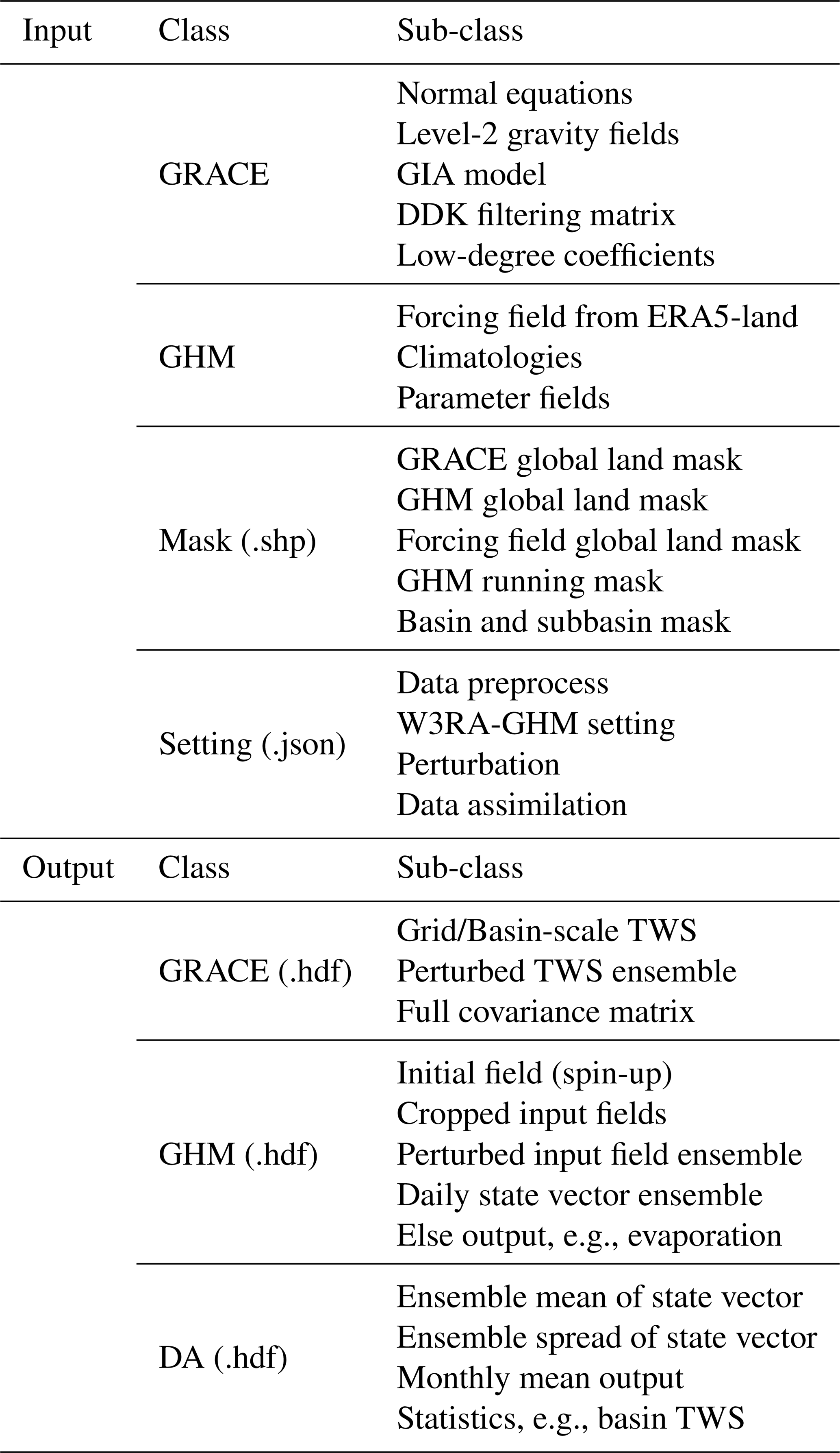
Please refer to Table B1 for a record of the input and output of the software. Details on the inputs (GRACE, GHM, and Mask) can also be found in Sect. 2. Information on the setting files (.json) can be found on our Github or in the data repository (Yang, 2024). The output can also be obtained by running the demo offered in that repository.

Table B1 A summary of input-output of PyGLDA.