SanDyPALM v1.0: static and dynamic drivers for the PALM model to facilitate urban microclimate simulations

This study presents SanDyPALM, an innovative toolkit designed to streamline the generation of both static and dynamic input data for the PALM model, thereby facilitating urban microclimate simulations. SanDyPALM is capable of processing a diverse range of custom input data from raster and vector files, and it incorporates two novel methods – OSM2PALM and LCZ4PALM – that introduce the automated extraction of static input data from open data sources. To investigate the impact of static input data on simulation outcomes, we developed static drivers from four distinct data sources. Our analysis reveals not only variations in the generated static drivers but also differences in the simulation results. Importantly, all simulations correlate well with measurements from two different weather stations, underscoring the robustness of the overall modeling approach. However, we observed variations in temperature, humidity, and wind speed that are dependent on the static input data. Furthermore, our findings demonstrate that automated processing methods can yield results comparable to those achieved through expert-driven approaches, significantly simplifying workflows.

1 Introduction

Rapid urbanization and climate change are two significant factors that drive the need for a better understanding of urban climates. According to the Sixth Assessment Report of the IPCC (Pörtner et al., 2022), “an additional 2.5 billion people are projected to live in urban areas by 2050”. The report also states that “there is at least a greater than 50 % likelihood that global warming will reach or exceed 1.5 °C in the near term, even for the very low greenhouse gas emissions scenario”. In cities, the detrimental impacts of climate change will be intensified by the urban heat island phenomenon (Pörtner et al., 2022). To mitigate these adverse scenarios, urban microclimate analysis is crucial for effective urban planning.

One approach to analyze the urban microclimate is through the use of dense monitoring networks in urban areas. However, a significant drawback of this method is the practical challenge of ensuring adequate temporal and spatial coverage (Afshari, 2023). An alternative to direct measurements is microscale modeling, which enables comparative analysis of different scenarios and allows for the investigation of a large number of points in space and time (Toparlar et al., 2017).

The PALM (PArallelised Large-eddy simulation Model for Urban applications) model system (Maronga et al., 2020) has been increasingly utilized due to its accurate large eddy simulation (LES) core, which is based on the non-hydrostatic, filtered, incompressible Navier–Stokes equations, where buoyancy is considered using the Boussinesq approximation. It incorporates an internal self-nesting capability developed by Hellsten et al. (2021), as well as an offline-nesting capability implemented by Kadasch et al. (2021), which enables simulations to be driven by a mesoscale model. The PALM model system features PALM-4U, a suite of specialized components designed for detailed modeling of urban climate physics. Key components of this framework are (1) an urban surface model (Resler et al., 2017), (2) a land surface model (Gehrke et al., 2021), (3) a plant canopy model (see Maronga et al., 2020), (4) a radiative transfer model (Krč et al., 2021), (5) a building indoor climate model (Pfafferott et al., 2021), (6) an atmospheric chemistry model (Khan et al., 2021), and (7) a biometeorology model (Fröhlich and Matzarakis, 2020).

While the PALM model enables realistic urban microclimate simulations, its setup can present significant challenges. A substantial number of input data must be collected and formatted for both the static driver, which contains all static geographic information such as terrain height, building height, and land surface classification, and the dynamic driver, which includes transient initial and boundary conditions derived from mesoscale data. The PALM model establishes a comprehensive standard for input data, the PALM Input Data Standard (PIDS) – see PALM model system developers (2025a), and provides checks to ensure correctness and consistency. However, the preparation of input data remains a hindrance for researchers and users of the PALM model, which has been acknowledged in the community; see, e.g., Lin et al. (2024). This results in a need for user-friendly, semi-automated processing tools to facilitate data preparation, as manual techniques are impractical for large city-scale simulations. The following state-of-the-art review examines recent advancements and applications of static and dynamic drivers, referencing key literature and public software tools.

To create a static driver, the workflow provided by the PALM model environment utilizes the tool “palm_csd” along with geospatial input data that were preprocessed for the three German cities – Berlin, Hamburg, and Stuttgart – by Heldens et al. (2020) as part of the “MOSAIK” project, which was included in the first phase of the [UC²] project (Scherer et al., 2019). There are minimum requirements for basic simulations, with additional data available for more detailed and complex studies. Various sources of geospatial data were utilized: remote sensing data for building heights derived from lidar (light detection and ranging) and land cover classification from satellite imagery; municipal data collections, including building registries with detailed information and land use maps; and open data sources such as OpenStreetMap (OSM), which provided basic building footprints and street networks. A key limitation of “palm_csd” is its predefined data format, primarily designed for the “MOSAIK” dataset. Adapting it to other locations or data sources requires significant effort, as the data must first be manually processed into the required format.

Besides “palm_csd”, other static-driver tools have been developed. The following two packages have not been published, but the code repositories are publicly available: the first is “palmpy” (Fluck, 2023), a Python package that creates static drivers for the PALM model with comprehensive documentation, and the second is “rpalm” (Stadler, 2024b), an R package designed to create and edit static drivers for the PALM model.

To alleviate some of the existing limitations of default methods for creating a static driver, Lin et al. (2024) introduced GEO4PALM, an open-source toolkit that streamlines the processing of geospatial data from raw input to PALM-ready formats. It can utilize open data sources directly and includes tools for preprocessing and visualizing data.

Another static-driver tool, PALM-GEM, has been published by Bureš and Resler (2024), and it utilizes the publicly available data from UrbanAtlas, OSM, and EU-DEM. The tool has already been applied to develop a model for integrated urban services by Esau et al. (2024).

The “PALM-4U GUI” (Winkler et al., 2023) is a cloud-based graphical user interface (GUI) for the PALM model. The code is open-source and can be accessed via a code repository (Stadler et al., 2024a). The GUI provides a user-friendly way to prepare input data and simulation setups. Users can run, visualize, and analyze simulation results without requiring code writing. This method can be particularly helpful for new users or those unfamiliar with command-line interfaces, making it the easiest option for getting started with the PALM modeling workflow. Input data are created via an interactive web map editor, representing the area to be simulated as a polygonal city model. Geographic data can be imported, modified, and supplemented with user-drawn objects. Settings can be configured for global parameters and for each individual map object up to Level of Detail 2 (LOD2). City models can be created from OSM and translated into the PALM input data types using the open-source package OSM2PALM (Stadler, 2024a). The optional QGIS plugin “PALMClassify” (Stadler et al., 2024b) can classify custom geodata in shapefile format into PALM input data types and export them to the PALM-4U GUI.

Dynamic drivers provide transient boundary conditions to run the PALM model in “offline-nesting” mode, meaning that the PALM boundaries are defined using data from an external model. This approach can significantly improve the model's responsiveness to temporally varying large-scale atmospheric conditions and generally enhance the overall fidelity of the simulations. A major challenge in using dynamic drivers is the inherent errors in the weather prediction models themselves, which propagate into the PALM simulations and affect their accuracy (Radović et al., 2024).

The first method to create dynamic drivers from mesoscale models was INIFOR (Mesoscale Interface for Initializing and Forcing), developed by Kadasch et al. (2021). It has become the standard tool for dynamic-driver creation in PALM and interfaces with the mesoscale weather prediction model COSMO (Baldauf et al., 2011). INIFOR processes meteorological data (wind, temperature, humidity) and initial soil data from the weather prediction model, preparing them for use as dynamic boundary conditions in the PALM simulation. PALM utilizes the prepared data to set the conditions at its borders (top, sides, and bottom), ensuring that the smaller-scale simulation within PALM aligns with the larger-scale atmospheric processes.

Besides INIFOR, other methods have been developed to create dynamic drivers from mesoscale models, particularly for the Weather Research and Forecasting (WRF) model (Skamarock et al., 2019). The first was the “wrf_interface” presented by Resler et al. (2021), and it was used for a comprehensive study of realistic urban microclimate simulations. However, one downside of this approach is that it does not provide a surface layer model to fill the atmospheric data in the region below the first WRF model level.

Lin et al. (2021) introduced WRF4PALM – a tool designed to facilitate the conversion of mesoscale data from the WRF model into a dynamic driver. It implements a surface layer extension to fill data below the first WRF level using a simple logarithmic fit function.

Vogel et al. (2022) presented a new method for coupling the WRF mesoscale weather model with the PALM microscale model to simulate urban microclimates under realistic atmospheric conditions. The novel dynamic coupling scheme incorporates a roughness-corrected Monin–Obukhov surface layer representation (Arya, 2001), accounting for the varying roughness of urban surfaces to improve the accuracy of the initial and boundary conditions for the PALM model. This scheme is particularly important for WRF setups with relatively large vertical grid spacing near the surface. Simulations were conducted in an urban district of Berlin to test the new coupling scheme and investigate different WRF setups. The results were compared to standalone WRF simulations (without the microscale model) and actual measurements from the area. The main findings indicated that PALM simulations generally showed better agreement with measurements than standalone WRF simulations, especially for temperature. Refining the coupling time step or the WRF grid spacing did not significantly improve accuracy.

Radović et al. (2024) also used the WRF model to force the PALM model and described the challenges of establishing ideal conditions for running accurate simulations. The study determined that the accuracy of the model's results heavily relies on the quality of the boundary conditions. It was observed that errors or limitations in WRF data can significantly affect the results generated by PALM, although the influence of boundary conditions on PALM simulations can vary depending on the season and even the time of day. PALM can, to some extent, mitigate the impact of errors in wind speed from the boundary conditions. However, its ability to handle temperature variations arising from these errors is less consistent. Overall, the study emphasizes the crucial role of carefully chosen and high-quality boundary conditions in achieving reliable results with PALM.

Finally, the PALM model system release 24.04 (PALM model system developers, 2025b) features a new dynamic-driver creation tool named PALM-METEO, which is the successor of the “wrf_interface” by Resler et al. (2021). PALM-METEO supports a range of mesoscale models including WRF, ICON, and Aladin.

The study of the state of the art revealed that the options for creating PALM input data have been continuously increasing. However, several questions remain: (1) how can the process of input data preparation be accelerated and made more user-friendly? (2) What level of detail is necessary in the input data to produce realistic urban microclimate simulations? (3) How can we develop models on coarse grids, for instance, for a large parent domain that is driven by a mesoscale model?

In this paper, we present a workflow and the necessary program code to create static and dynamic input data for PALM simulations as an all-in-one solution. We primarily investigate how the level of detail in the geographic input data impacts the simulation results. Additionally, we introduce two novel methods, OSM2PALM and LCZ4PALM, to generate static drivers from OSM or local climate zone (LCZ) maps anywhere in the world. LCZ4PALM is particularly useful for parametric studies and for coarser grids, where real building shapes cannot be resolved, making it preferable to have an approximate but meaningful urban representation instead. In this work, we compare four static drivers from different data sources: (1) “MOSAIK” – the dataset by Heldens et al. (2020), which has already been preprocessed but still needs to be converted into a static driver; (2) “Custom” – our own custom preprocessing of data openly available from the municipality; (3) “OSM” – data preprocessed by our tool OSM2PALM; and (4) “LCZ” – data preprocessed by our tool LCZ4PALM. The four simulation variations were conducted, validated by tower and station measurements, and then compared to each other to address our stated research questions.

The findings of this study indicate that the choice and quality of input data influence the accuracy of urban microclimate simulations using the PALM model. By comparing various static drivers derived from different data sources, we demonstrate how variations in data representation can lead to differences in simulation outcomes, particularly in temperature, humidity, and wind speed. Despite these differences, all simulation test cases could be validated using measurement data, albeit with varying degrees of deviation. The introduction of the novel methods, OSM2PALM and LCZ4PALM, to generate static drivers from widely available geospatial data enhances the accessibility and applicability of urban climate modeling. Ultimately, this research contributes to the development of more reliable urban climate simulations, which are essential for informed urban planning and effective climate change mitigation strategies.

2 Methodology

The methodology consists of five parts: the first in Sect. 2.1 describes the simulation test case defined for our investigation. The next section, Sect. 2.2, outlines the various geographic data sources and explains how the data were preprocessed before generating the static driver. Section 2.3.1 provides a detailed account of the static-driver generation process, while Sect. 2.3.2 briefly describes the dynamic-driver creation. In Sect. 2.4, we present our specific PALM setup, including grid and model settings. Finally, the measured data from a tower station, which we used for validation in this study, are presented in Sect. 2.5.

2.1 Test case

The time period of our test case spans 2 d, from 19 July 2022 00:00 until 21 July 2022 00:00 central European summertime (CEST). This 2 d period was characterized by a heat wave with record-breaking temperatures in Germany and other European countries. According to ERA5 reanalysis data evaluated for the region around Berlin, the average temperature over the 2 d was 28.0 °C, with temperature maxima of 35.4 °C on 19 July and 37.9 °C on 20 July. The wind speed was relatively low, with an average value of 2.2 m s⁻¹, and the wind direction was predominantly southeast. The period was cloud-free, with total cloud cover not exceeding 1 % over the 2 d span.

Our test case uses nested domains to cover an overall larger area with the parent domain while allowing a sufficiently high resolution in the nested domain around the main region of interest. The location of our test case is in the borough of “Steglitz-Zehlendorf” in Berlin, Germany. The average terrain height in the region is 46 m. The simulation domains are centered at the weather monitoring tower situated in the garden of the Institute of Ecology at the Technical University of Berlin (TUB). We chose this location specifically because it offers a high quantity and quality of measurements, allowing for thorough validation of our simulation models. In addition to the tower, there is also a measurement station of the German Weather Service (DWD – Deutscher Wetterdienst) in “Dahlem”, which is covered by the parent domain and can therefore also be used for validation.

SanDyPALM facilitates the selection of coordinates and domain size by offering a function that calculates the coordinates in both latitude/longitude and the PALM native grid, which is a local projection. It also plots the parent and all nested domain borders over a geographic map. Our test case is visualized in this manner in Fig. 1.

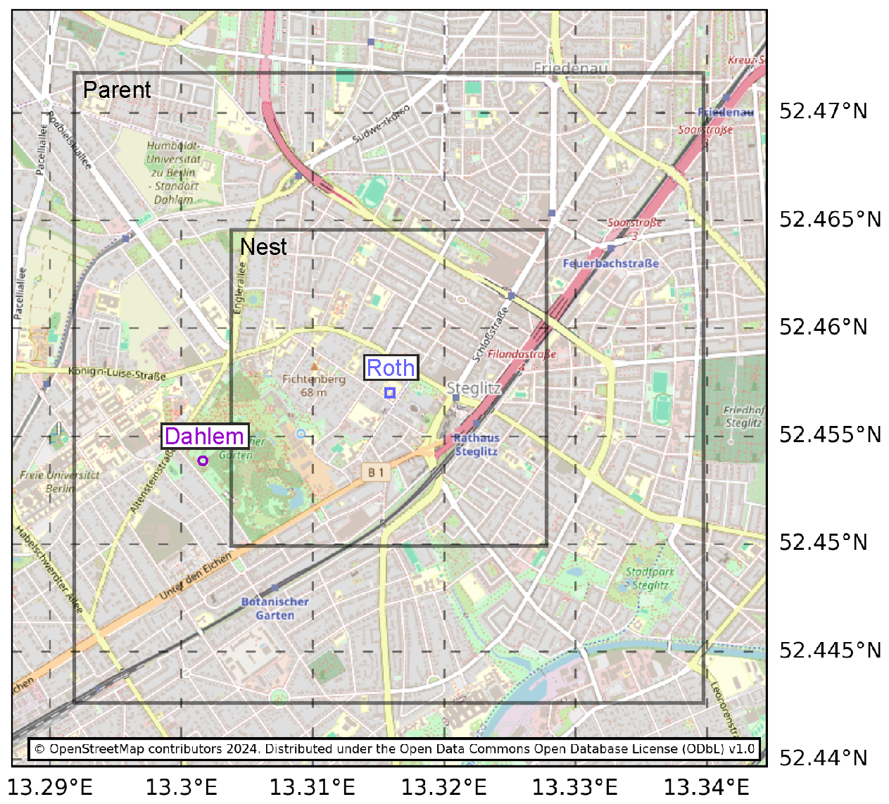
Figure 1 Open street map (OpenStreetMap contributors, 2024) of the test case with illustrations of the domain outlines of the parent and nested grids. The map also indicates two measurement locations used in this study: the TUB tower in Rothenburgstraße “Roth” and the DWD station in Botanischer Garten “Dahlem”.

The local coordinate system we use for this test case is EPSG:25833, a universal transverse mercator (UTM) projection for zone 33N. The center coordinates of our domain are 52.457227° N, 13.315827° E (latitude/longitude) or y=5813228.0 m, x=385566.5 m (EPSG:25833). In SanDyPALM, the coordinates can be specified in four different ways: (1) native PALM coordinate system of the domain center, (2) latitude/longitude of the domain center, (3) native PALM coordinate system of the domain lower-left corner, and (4) latitude/longitude of the domain lower-left corner.

2.2 Geographic data sources

The SanDyPALM package allows input from different data representations, which mainly include (1) raster data stored in netCDF format, (2) raster data stored in GeoTIFF files, and (3) vector data stored in commonly used formats, such as ESRI Shapefile, GeoJSON, or GeoPackage. In this work, we aim to prepare one test case with different data sources and compare how the static driver varies depending on the data source and how this affects the simulation results. We defined four data sources for our test case in Berlin. The first is the data generated within the MOSAIK project, which are readily preprocessed as netCDF raster files. The second is our own custom preprocessing of openly available data from the municipality of Berlin. The third is a dataset derived from generally available open data sources, mainly OSM, which requires special preprocessing to convert the data types into a format compatible with PALM. The last source differs from the others in that it does not represent the actual urban geometry but instead derives a virtual city solely from a 100 m LCZ map using our tool LCZ4PALM. Geographic maps of the different data sources are presented in Fig. 2, where selected data types are illustrated in different colors. Table 1 summarizes the main differences between the data sources; detailed descriptions of each data source follow in the next four sections.

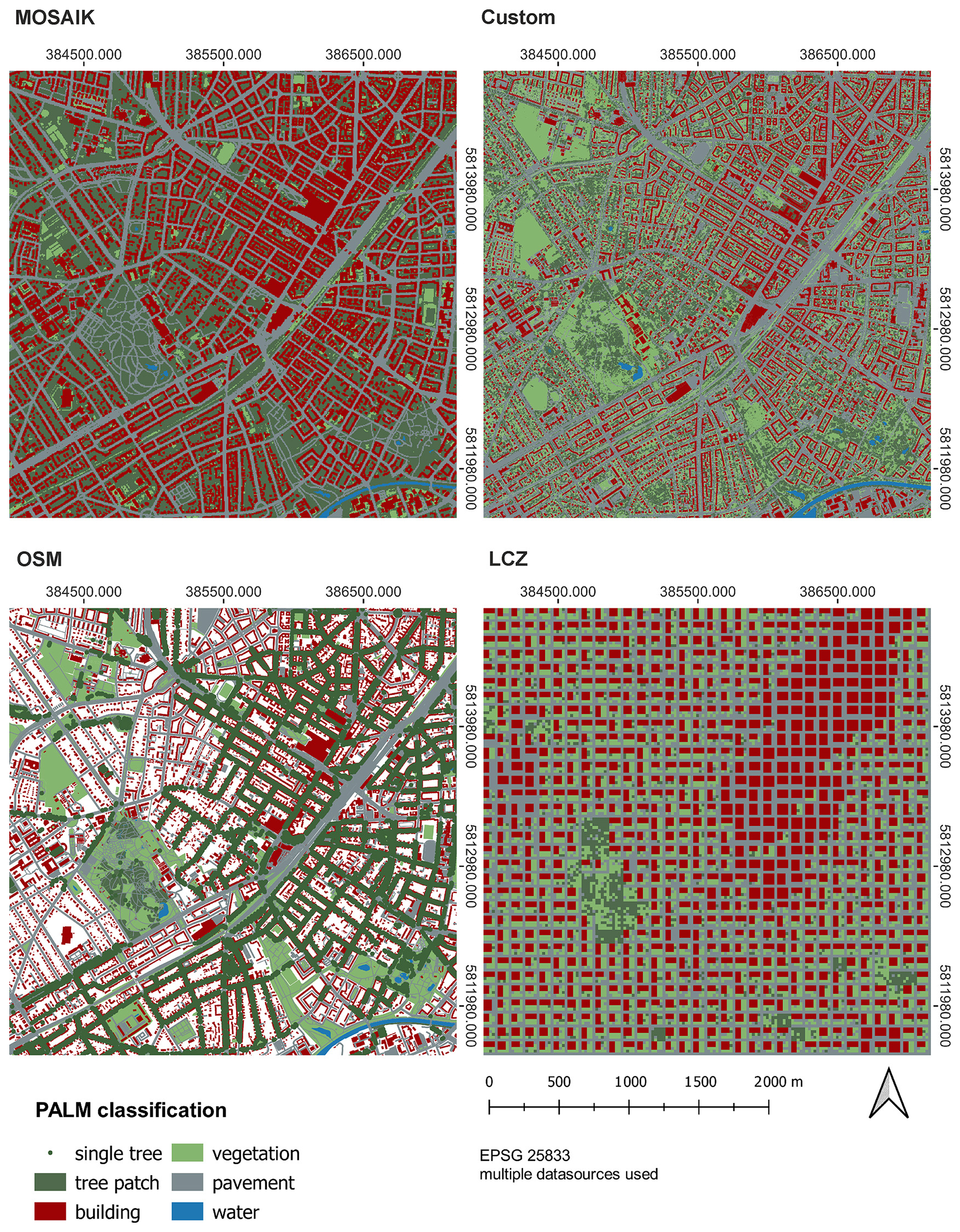
Figure 2 Geographic maps of the four different input data sources for SanDyPALM.

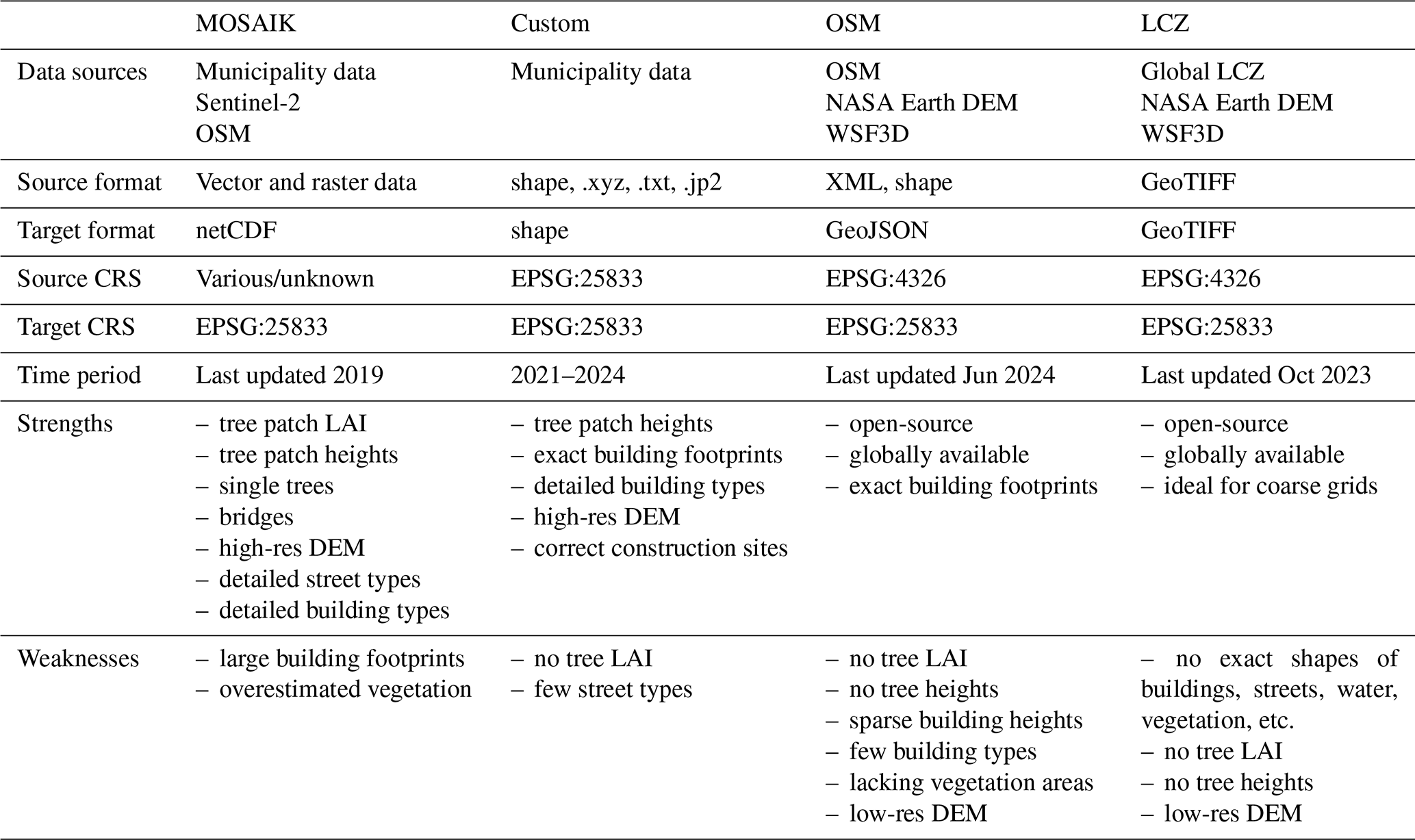
Table 1 Comparison of the four different input data sources used in SanDyPALM to generate static drivers. The following abbreviations are used: OSM, OpenStreetMap; DEM, digital elevation model; WSF3D, World Settlement Footprint 3D; LAI, leaf area index; CRS, coordinate reference system.

2.2.1 MOSAIK

This dataset originates from the MOSAIK project, for which several data sources were preprocessed for use in the PALM model. This dataset was intended to be further processed and converted into a static driver by the utility palm_csd that is shipped with the PALM model. However, in this work, we used SanDyPALM instead to convert this dataset into a static driver. For a detailed description of the MOSAIK dataset, we refer to Heldens et al. (2020).

2.2.2 Custom

The “Custom” dataset contains openly available data from the municipality of Berlin, specifically from the geodata portal run by the Senate Department for Urban Development, Building and Housing of Berlin. The data to be used were selected after an in-depth search on the portal for information compatible with PALM types.

The data were processed using our own custom processing based on Heldens et al. (2020) and the workflow proposed for “PALMClassify”. This resulted in a dataset where each PALM type is represented by one shapefile, including information on covered area, specific type, building height, and tree height.

Often, multiple input datasets represented parts of the same PALM type, necessitating their combination. In some instances, new datasets had to be created; for example, the true orthophoto channels of red and near-infrared were used to calculate the NDVI (normalized difference vegetation index), which helped identify vegetation and tree areas. The topography and the digital surface model were used to create the normalized digital surface model, which provided height values for buildings and trees.

2.2.3 OpenStreetMap

Input data for PALM can also be created using OSM (OpenStreetMap contributors, 2024). It contains surface classifications, building footprints, building heights, and trees. Data quality varies by region, but for European cities, it is relatively high. For more information on the completeness of building data in OSM, we refer to Herfort et al. (2023).

OSM has an open API that allows filtering data on the server side to reduce the number of data received from OSM. However, experience has shown that requesting the entire OSM chunk yields the most detailed datasets because useful information can be found in any group and definition provided by OSM.

A Python package called OSM2PALM (Stadler, 2024a) has been developed to request and process OSM data. It primarily uses lookup tables defined by Heldens et al. (2020), with minor adjustments to existing tables and new value pairs for previously unused OSM attributes. Continuous efforts are made to search for and identify unused OSM surface classifications that can be reasonably translated into PALM surface types.

One advantage of OSM data is their detailed representation of features outside cities, including forests, shrubs, and small rivers. In urban areas, building footprints and unique features like swimming pools and parks are accurately depicted, but surface data are often insufficient. While roads can be estimated using buffered line datasets, information on sidewalks and the front and back yards of buildings is typically lacking.

Some data needed for PALM, like building and tree heights, are often absent in OSM. The missing data are handled as follows: if the building height is unavailable, the number of stories is used to estimate it with a constant story height. If neither the building height nor the number of stories is found, a default height is assumed by OSM2PALM. To fill these missing building heights, we used the global building height data of the World Settlement Footprint 3D (WSF3D) generated by Esch et al. (2022). All default heights previously set by OSM2PALM were replaced using the WSF3D raster data interpolated onto the center points of the building footprints. This way, every building in the OSM method obtains a reasonable building height, albeit with varying accuracy. For trees with missing heights, a default of 12 m is used.

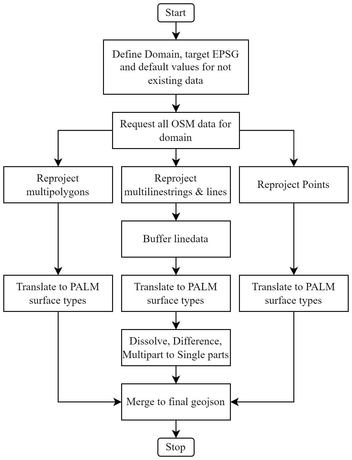
The general workflow of the OSM2PALM script can be seen in Fig. 3. It begins by requesting all data from OSM, converting them into a UTM coordinate system, and grouping them into three categories: multipolygons, line data, and points. Multipolygons and points are translated according to a lookup table. Single values from an attribute or information from the other_tags attribute are used to define the PALM surface type and its value. Line data require further processing, including buffering, dissolving, and creating differences; typical examples includes roads, train tracks, and small rivers. Finally, all datasets are merged and saved as a GeoJSON file.

Figure 3 Workflow of conversion from OSM data into PALM input data.

2.2.4 Local climate zones

This dataset for the static driver is obtained using our tool “LCZ4PALM”. It is a novel feature incorporated into SanDyPALM to create a static driver using the global LCZ map provided by Demuzere et al. (2022). PALM requires a detailed description of urban and rural neighborhoods for accurate microclimate modeling and analysis. Unfortunately, this information is neither readily available nor easily accessible for every region in the world, which severely limits the ability to perform microclimatic studies. The static data are usually obtained from multiple sources and involve extensive preprocessing, as outlined in the previous sections. This problem is addressed with the help of globally available LCZ maps. LCZs are defined by Stewart and Oke (2012) as “regions of uniform surface cover, structure, material, and human activity that span hundreds of meters to several kilometers in horizontal scale”. LCZ is the most popular landscape classification scheme and is widely used in climate simulations and related studies. It mainly focuses on the classification of urban and rural landscapes (17 classes – 10 built classes and 7 natural classes) based on surface characteristics such as building packing densities, aspect ratio, building or tree height, sky view factor, surface albedo, or anthropogenic heat emissions. This makes it highly suitable for urban microclimatic studies, typically investigations of the urban heat island effect.

Demuzere et al. (2022) generated a global map of LCZs at a 100 m resolution by training a random forest model using a large labeled dataset. In our tool, these LCZ maps are first reprojected onto the PALM simulation domain, and the LCZs corresponding to the intended simulation region are extracted. Then, for each LCZ tile, geospatial inputs (buildings, vegetation, waterbodies) that conform to the LCZ definitions are generated in a systematic approach, as shown in Fig. 5. Using this method, we construct an idealized city with buildings, vegetation, and pavements, which can be used as an alternative for realistic domains. This approach is mainly suitable for coarse grids with a grid spacing above 10 m, for either parent domains in nested setups or generic LCZ studies of large areas where coarse grids are needed to limit computational effort. The problem is that at low resolutions, realistic buildings, trees, and pavements are often either overestimated or underestimated. For example, narrow streets may disappear, while wider streets are stretched to fit the entire grid cell. The same applies to buildings and vegetation. This leads to unrealistic inputs that negatively impact simulation accuracy. The virtual city created by LCZ4PALM may not be accurate in its details, but it represents the urban morphology on average.

The process is shown in Fig. 4. The LCZ4PALM module requires several inputs, including an LCZ map that covers the desired region, a mapping of PALM type probabilities to LCZ classes (building types, pavement types, vegetation types, and vegetation properties), the LCZ definitions, and, optionally, a global building height dataset. The mapping of PALM type probabilities is not directly available and needs to be derived from another data source. In this study, we performed an exemplary analysis using a 30 km by 30 km region around Berlin from the MOSAIK dataset by Heldens et al. (2020) to generate these data. For each LCZ class, the probability of occurrence of all PALM types was derived. The resulting mapping was saved in a JSON file and is valid for Berlin and cities similar in urban morphology. The LCZ definitions used in this study were provided by Stewart and Oke (2012). For each LCZ class, they specify a range for surface fractions, which include building surface fraction (BSF), pervious surface fraction (PSF), impervious surface fraction (ISF), aspect ratio, and building height. To achieve more accurate building heights, we used the global building height data of WSF3D (Esch et al., 2022). Alternatively, random building heights within the LCZ range can be used. Before generating the static driver, the input data undergo several preprocessing steps. Initially, the global LCZ map is projected onto the PALM grid using a resolution specified by the user. Next, it is resampled onto an LCZ grid with a resolution of at least 100 m using a custom grid-resampling technique. This technique assigns the LCZ value with the highest occurrence to the grid cell. Finally, once the LCZ grid is prepared, the code generates the geospatial information for each LCZ tile.

Figure 4 Process diagram of the LCZ4PALM algorithm.

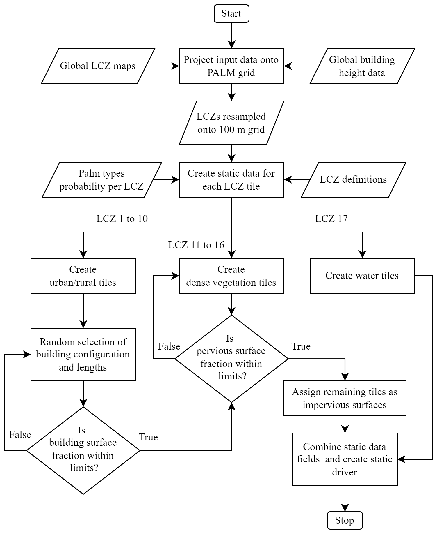
The approach of generating a virtual urban neighborhood from LCZ classes is illustrated in Fig. 5. The grid cell size is 20 m in this case. The virtual city is created in blocks of 100 m by 100 m, and for each of these blocks, a dominant LCZ class is assigned and urban surfaces are generated, while different functions are used depending on the LCZ class. For built types ranging from LCZ 1 to 10, building, pavement, and vegetation tiles are created. One row and one column of pavement tiles are always allocated in the southern and eastern borders. The available length and width of the buildings are utilized to compute the maximum number of buildings that can be accommodated without violating the LCZ class specification. This information is then used to determine the potential configurations of aligned arrays of cuboidal buildings. For instance, this could involve arrangements such as 2×3 or 2×1 building tiles, among others. From the various possible configurations, one configuration is chosen randomly, provided that it satisfies four conditions. These conditions comprise ensuring that the building surface fraction, total length, and total width of buildings, as well as the length-to-width ratio of the buildings, all meet the requirements of the LCZ class. The building surface fraction condition is determined based on the LCZ definitions and must fall within a specified range of minimum and maximum values. Furthermore, the total width and length of the buildings and streets should be smaller than the total width and length possible for the given tile. To prevent the presence of long and slender buildings in the domain, a maximum length-to-width ratio of 4 is enforced. Once all of these conditions are met, the building array is generated for the LCZ grid.

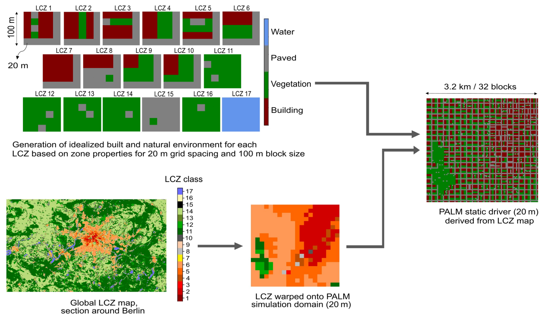
Figure 5 Creation of geospatial input data for the PALM model using LCZ4PALM with global LCZ maps.

The subsequent step involves creating vegetation around the buildings up to a randomly determined limit within the permissible range. The remaining tiles that are not part of the buildings are designated as vegetation tiles until the criteria for the pervious surface fraction are met. Once the vegetation tiles are marked, each tile needs to be assigned a vegetation type, for which the corresponding vegetation properties can be further defined. This is accomplished using the data obtained from the PALM type probabilities per LCZ discussed earlier, which include the vegetation type along with its probability of occurrence. For each vegetation tile, a vegetation type is randomly sampled based on its given probability and is assigned to the tile. The vegetation types can be categorized as either high or low, depending on the characteristics of the vegetation present. In the case of a high vegetation type (4, 5, 6, 7, 17, or 18), additional information such as tree patch height and leaf area index (LAI) is required. The PALM type probability mapping also contains the mean and standard deviation of tree heights in the Berlin region for each vegetation type within each LCZ. Using this information, the tree patch height is calculated from a random normal distribution.

After creating the vegetation, the remaining tiles are utilized to create impervious surface elements (streets and pavements). Building types and pavement types are assigned to the corresponding tiles in a manner similar to that of vegetation types.

For land cover types ranging from LCZ 11 to 16, the creation of vegetation and pavement tiles follows the same process as explained earlier. However, in this case, there are no buildings present. Therefore, only the criteria for pervious and impervious surface fractions are satisfied. For water (LCZ 17), water tiles are currently created using a default type 4, which corresponds to ponds. However, this type can also be modified to a user-defined type based on the domain. All of the data needed for static-driver generation are saved as GeoTIFF files for later processing into a static driver using SanDyPALM.

2.3 SanDyPALM package

The new open-source repository SanDyPALM consolidates our efforts to create static and dynamic drivers for PALM using Python code. It is a collection of steering scripts and functions that are intended to run in the command line or in an integrated development environment (IDE). The majority of the static-driver generation code originates from the PALM-4U GUI (Winkler et al., 2023), while the WRF dynamic-driver code has been developed and utilized by Vogel et al. (2022). SanDyPALM is a package that can generate all necessary input data for a WRF-driven microscale simulation setup. However, it can also be used to create only a static driver for unforced PALM simulations or for combining it with a different dynamic-driver tool. Also, it can be used to only create a dynamic driver for an existing static driver. The static and dynamic drivers are created according to the PIDS (PALM model system developers, 2025a).

SanDyPALM comes with a default configuration and a set of tutorial scripts that explain the basic setup and guide the user through the complete process of creating a static driver from various geographic data sources, as well as creating a dynamic driver using WRF data. Further tutorials detail the basic plotting of results and conversion of input data between netCDF, GeoTIFF, and vector formats. In addition to tutorials, we also included example case files, where each script directs one complete generation process. All our PALM setups are nested cases and relatively small, allowing them to be run without high-performance computing. The configuration always starts from a predefined default configuration that is modified in a tutorial or case file. The final configuration is always saved together with the static and dynamic drivers to enable the user to retrace the settings with which the drivers were generated. SanDyPALM encourages users to work in projects, where each project contains all generated data, configuration parameters, and generated plots.

SanDyPALM also facilitates nesting and grid setup by offering a simple and independent function to generate the PALM grid positions before performing any time-consuming processing. The grid positions are first generated as local coordinates and then transformed into the user-specified geographic coordinate reference system. All nested domains can be plotted together on an OSM to inspect their sizes and positioning. The grid extent in the three dimensions, as well as all vertical grid levels and thicknesses, is printed to the terminal. This allows the user to quickly test different grid settings and optimize the vertical grid stretching parameters.

Once the domains are finished, open data can be automatically downloaded from several available data sources. There is an interface to OSM2PALM (the code for OSM2PALM needs to be downloaded separately) that can be used to download OSM data for the given extent of the largest domain. Another interface allows downloading the ASTER Global Digital Elevation Model V003 with a resolution of 30 m from NASA Earth Science data (ASTER Science Team, 2019) using the Python package earthaccess in the background. The data are freely available but require registration. SanDyPALM provides an HTTP interface to download other needed files into an appropriate data folder. In our tutorials, the global LCZ map (Demuzere et al., 2023) and the WSF3D building heights (Esch et al., 2022) are automatically downloaded if desired. The LCZ map is needed for the LCZ4PALM module, and WSF3D can be used in both LCZ4PALM and OSM2PALM to provide approximate building height information for better accuracy.

2.3.1 Static-driver generation

The static driver represents a domain in a Cartesian grid using raster data. A definition of all possible input data fields is given in the PIDS (PALM model system developers, 2025a). Depending on the application of PALM, the mandatory data fields in the static driver vary; for example, in the case of boundary layer studies, only the roughness length of the surface is needed. For an urban simulation, more information is required, such as surface classifications, topography, and building positions and heights. PALM uses four major surface classifications: vegetation, pavement, water, and buildings, each with sets of predefined physical parameters, such as roughness for heat and momentum or albedo. For each grid tile in the domain, these parameters can also be adjusted from the predefined values. There are two major 3D datasets that interact in the atmosphere: 3D buildings and leaf area density (LAD). The 3D building data define a grid of ones and zeros, where ones represent building grid points and zeros represent atmospheric grid points. These data can be used to model overhangs, gates, or bridges. The LAD dataset is used to model the 3D influence of trees, which interact with radiation and humidity in the atmosphere and act as a momentum sink.

SanDyPALM is able to create a static driver that follows the PIDS requirements and performs further processing for certain datasets or according to the settings of SanDyPALM. A major feature of SanDyPALM is the support for multiple types of geospatial data. Typically, geospatial data are either vector data using polygons (i.e., surfaces, lines, and points) or raster data using a grid format. SanDyPALM can read many vector formats (shapefile, GeoJSON, SQLite, GeoPackage), the GeoTIFF format, or the netCDF datasets specifically defined within the MOSAIK project (Heldens et al., 2020). The data are then rastered or resampled onto the grid defined by the user and written to the static driver. Each input file needs to be assigned to a surface classification of PALM or set predefined names for processing. Depending on the input file type, further information and settings must be provided. The static-driver generation method is visualized in the flowchart in Fig. 6.

Figure 6 SanDyPALM static-driver generation flowchart.

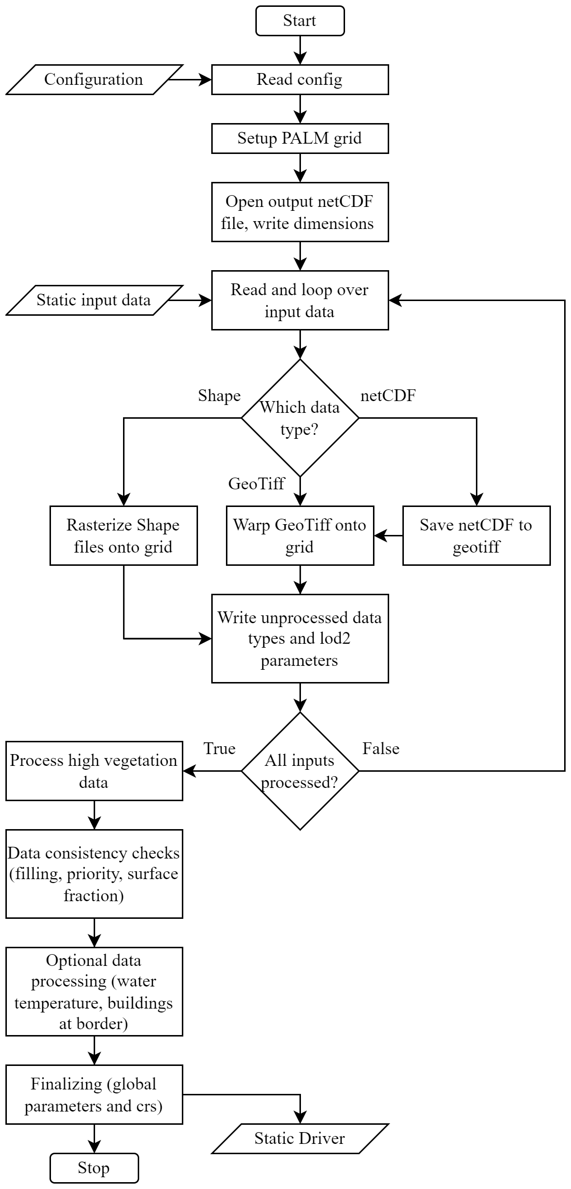
Shapefiles are converted into raster datasets via the rasterize function of the GDAL Python package. Besides the domain definition, this function also requires the attribute that is to be rastered. Optional inputs include an attribute filter as well as a rasterization parameter that specifies when grid tiles are considered inside or outside of a polygon that is to be rastered (“all touched”).

GeoTIFF files are resampled onto the defined grid via the “warp” function of GDAL. Typically, the raster band of the desired dataset should be specified; otherwise, SanDyPALM takes the first band (0) by default. If the resolution of the dataset differs from the target resolution of the static driver, a resampling or aggregation algorithm can be defined in the GDAL “warp” function. The resampling algorithm needs to be chosen wisely based on the type of data and whether the data are up- or down-sampled.

The netCDF data that came from the MOSAIK project do not have their geo-referencing inside each data file; instead, additional files are needed that specify the x and y coordinates in a UTM coordinate system. SanDyPALM reads the data files as well as the coordinate files and first creates geo-referenced GeoTIFF files; then they can be resampled using GDAL tools similarly to the GeoTIFF files.

For the urban surface parameterizations, it is expected that the provided data are already translated into the PALM surface types with the corresponding sub-types. Data for these parameters are converted to the grid and then saved directly onto the appropriate PALM variable. Level of Detail 2 (LOD2) parameters, such as roughness length of vegetation, can also be adjusted from 2D input files in a separate sub-dictionary of the configuration. The position of the 2D slice inside the 3D dataset must be provided as additional input.

Resolved vegetation can be implemented in the static driver using a 3D LAD field. There are two common methods to resolve trees: (1) single trees are resolved as 3D shapes and (2) groups of trees are modeled using vertical LAD profiles. Currently, only the second method is implemented in SanDyPALM following a similar approach to that in the tool “palm_csd”. However, SanDyPALM features a new discrete tree canopy generator, which asserts that the integral of the LAD profile is exactly the LAI value of the grid tile.

The leaf area distribution is defined according to Markkanen et al. (2003) in Eq. (1), which is a probability density function; therefore, we define this as normalized (denoted by the overline) LAD:

$$\begin{array}{}\text{(1)}& \stackrel{\mathrm{‾}}{\mathrm{LAD}}\left({\displaystyle \frac{z}{h}},\mathit{\alpha },\mathit{\beta }\right)={\displaystyle \frac{{\left(\frac{z}{h}\right)}^{\mathit{\alpha }-\mathrm{1}}{\left(\mathrm{1}-\frac{z}{h}\right)}^{\mathit{\beta }-\mathrm{1}}}{{\int }_{\mathrm{0}}^{\mathrm{1}}{\left(\frac{z}{h}\right)}^{\mathit{\alpha }-\mathrm{1}}{\left(\mathrm{1}-\frac{z}{h}\right)}^{\mathit{\beta }-\mathrm{1}}d\left(\frac{z}{h}\right)}}.\end{array}$$

This equation is then discretized on the PALM grid, replacing the integral with a summation over the vertical grid cells, which leads to the discretized version (denoted by the asterisk) of the normalized LAD profile given in Eq. (2):

$$\begin{array}{}\text{(2)}& {\stackrel{\mathrm{‾}}{\mathrm{LAD}}}^{\ast }={\displaystyle \frac{{\left(\frac{z_i}{h^{\ast }}\right)}^{\mathit{\alpha }-\mathrm{1}}{\left(\mathrm{1}-\frac{z_i}{h^{\ast }}\right)}^{\mathit{\beta }-\mathrm{1}}}{{\sum }_{i=\mathrm{0}}^{N_z}\left({\left(\frac{z_i}{h^{\ast }}\right)}^{\mathit{\alpha }-\mathrm{1}}{\left(\mathrm{1}-\frac{z_i}{h^{\ast }}\right)}^{\mathit{\beta }-\mathrm{1}}\right)\frac{\mathrm{\Delta }z}{h^{\ast }}}}.\end{array}$$

Here, z_i denotes the heights of the grid cell centers (above ground) and h^∗ is the discretized tree height of the current grid tile. The discretized tree height is calculated for each grid tile by rounding the tree height to the nearest staggered vertical position z_w (defined for vertical velocity) of the PALM grid. We use these grid positions because they are also the vertical grid cell faces (or boundaries) of the non-staggered grid cells.

The discretized non-normalized LAD profile LAD^∗ is then obtained by multiplying by the LAI and dividing by the discretized tree height h^∗ using Eq. (3):

$$\begin{array}{}\text{(3)}& {\mathrm{LAD}}^{\ast }={\displaystyle \frac{\mathrm{LAI}}{h^{\ast }}}{\stackrel{\mathrm{‾}}{\mathrm{LAD}}}^{\ast }.\end{array}$$

This equation is applied to every grid cell of the PALM domain. The formulation is fully conservative; if we integrate over all LAD values on top of one grid tile, we exactly obtain the LAI value of that grid tile. A check is in place to ensure that this is always the case.

While the tree height is a mandatory input for SanDyPALM, the LAI and α parameters can be obtained from a predefined default value if no appropriate data fields are available. The default LAI value can also be automatically scaled by tree height. Therefore, instead of using one default value for all trees, we define a default value for $\frac{\mathrm{LAI}}{h}$. From that, a more appropriate default LAI value can be derived for different tree heights. A typical default value would be $\frac{\mathrm{LAI}}{h}=\mathrm{0.2}$, which means that a tree of 5 m height would have a default LAI value of 1 and a tree of 25 m height would have a default LAI value of 5. For these default LAI values, the LAD is still calculated using Eq. (3). While this procedure is not highly accurate, it is superior to simply specifying one default LAI value.

We also implemented two different filtering strategies for LAI data fields after encountering relatively high LAI values. The first method limits the value of $\frac{\mathrm{LAI}}{h}$ to a threshold of, for example, 0.2. As a result, for each grid cell, the value of LAI is reduced so that $\frac{\mathrm{LAI}}{h}\le \mathrm{0.2}$. Alternatively (or additionally), we can check the final values of the 3D field of LAD^∗ and limit them to a certain value, e.g., 0.1.

SanDyPALM creates the 3D building data from the 2D building data, primarily for visualization purposes, since the PALM model itself constructs the 3D building data. However, to be able to add custom buildings into the 3D building data, we need to create the 3D building data beforehand. If the height of the custom building exceeds the height of all other buildings in the domain, we can set a user-defined maximum height for the 3D building data field to ensure there is enough space in the data field to add the building. This enables us to add specific buildings at a later stage after creating the static driver. For example, we used this procedure to add a custom model of the Berlin tower (Fernsehturm) in Vogel et al. (2022).

Another feature of SanDyPALM is that it performs automatic data consistency checks and allows the user to handle inconsistencies. These inconsistencies could be grid tiles that have no surface classification assigned (missing data) or grid cells with multiple classifications (overlapping data). After the initial assignment of surface parameters and building data to the static driver, all grid points are checked for missing data, and a default surface classification and value are assigned to these grid points. Afterwards, all grid points are checked for overlapping data, where a user-defined priority list is applied to decide which data field is to be kept. The default setting uses the following priority (descending): buildings, water, pavement, vegetation.

A data filter checks for specific values in data fields that can be replaced with a given value. We used this functionality to replace the building type “0” in the MOSAIK data, which stands for “user-defined”, for which the user would need to specify all LOD2 building parameters.

Another feature in SanDyPALM is to remove buildings at the border of the domain to adhere to typical guidelines for atmospheric boundary layer studies and to avoid potential discontinuities at the inflow of the domain. Within a defined number of grid cells from the domain edge, all buildings are automatically removed and replaced by pavement. We can further decide to remove all grid cells with the same building ID as already-removed buildings so that buildings are not cut into pieces but are removed entirely. In a nested setup, it makes sense to use this feature only in the outermost “parent” domain.

The soil type can be provided as a 2D input file, but if it is not available, a default value for the whole domain can be used. In any case, SanDyPALM handles the correct allocation of the soil type as well as the surface fraction variable. Finally, a domain-wide constant water temperature can be defined that is then applied to all waterbodies in the static driver.

2.3.2 Dynamic-driver generation

The dynamic-driver generation is the second main component for setting up a realistic urban microscale simulation using PALM. Currently, SanDyPALM supports WRF as the input data source. Using the WRF model has the significant advantage of allowing a relatively fine horizontal grid spacing on the order of 1 km, and it enables the use of an urban canopy layer scheme together with an urbanized land use/land cover map and optionally even average building heights to better represent urban effects in the mesoscale forcing. We believe that this leads to significantly improved boundary conditions for the PALM model. The process of creating the dynamic driver is illustrated in Fig. 7.

Figure 7 SanDyPALM dynamic-driver generation flowchart.

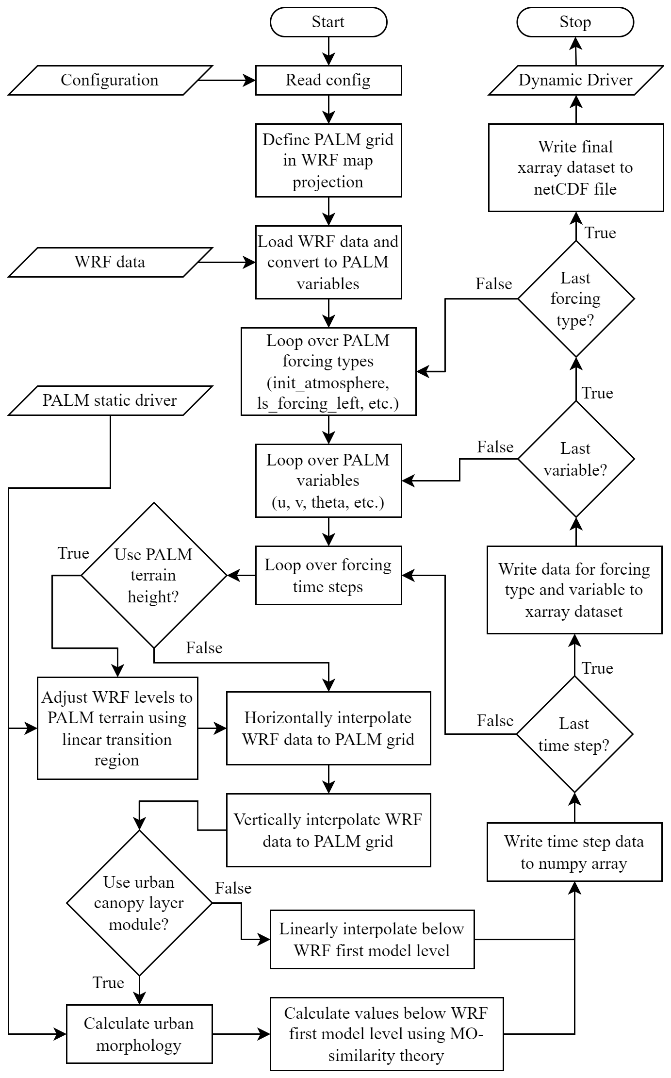
One novelty of our dynamic-driver creation is the handling of mesoscale data below the first model level of the mesoscale model. Since the data in this region are not available, we need to fill the gaps using reasonable values. As described in Vogel et al. (2022), our dynamic coupling scheme incorporates a roughness-corrected Monin–Obukhov surface layer representation, which accounts for the varying roughness of urban surfaces. As mentioned earlier, this scheme is important for WRF setups with relatively large vertical grid spacing near the surface, which are typically used together with the single-layer urban canopy model (SLUCM) or the slab (or bulk) urban model in WRF. With small vertical grid spacing near the surface in WRF, which is typically the case when using the multi-layer urban canopy model named building effect parameterization (BEP), a simple linear interpolation may be sufficient.

The dynamic-driver generation can utilize the building height data in the static driver to derive the urban morphological parameters needed in the aforementioned roughness-corrected Monin–Obukhov surface layer representation. Additionally, the terrain height can be read from the PALM static driver to adjust the atmospheric data from WRF to the PALM terrain height. To achieve this, the WRF level heights are shifted by the amount that the WRF terrain deviates from the PALM terrain. However, this shifting is limited to the surface so that we do not shift the atmospheric layers throughout the entire boundary layer. Therefore, we can specify a vertical distance for this transition region. The WRF level heights will then be fully shifted at the reference height, which is either the WRF first (half) model level height or a user-defined reference height to which the WRF data are interpolated. At the specified distance above the reference height, the WRF level heights will remain untouched. All level heights in between will be linearly shifted. This produces a smooth transition region and limits the level height shifting to a small area close to the surface. The procedure is illustrated in Fig. 8.

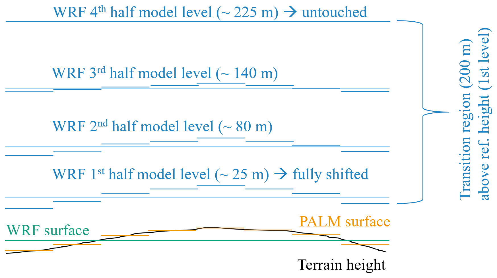
Figure 8 Adjustment of WRF mesoscale level heights based on the difference between WRF and PALM surface heights, which account for actual terrain elevation at different horizontal resolutions. The adjustment procedure employs a linear transition region. This example is illustrative and does not represent the actual level heights utilized in this study.

2.4 PALM setup

This section provides a short summary of our most important PALM model settings, which include offline nesting, the choice of grid, the solver, and the setup of the urban physics modules.

We used release 23.04 of the PALM model system from the Institute of Meteorology and Climatology Hannover, which can be obtained from their code repository (PALM model system developers, 2025b).

The PALM model is forced by mesoscale data using the offline-nesting capability. The mesoscale data are the result of a WRF downscaling simulation using three nested domains with spatial resolutions of 9, 3, and 1 km and a temporal resolution of 1 h. The WRF model was itself forced by ERA5 global reanalysis data (Hersbach et al., 2018a, b) with a spatial resolution of 0.25° in both latitude and longitude, which at the given latitude equates to approximately 28 km by 17 km, respectively, and a temporal resolution of 1 h. The WRF mesoscale simulation used here is similar to the setup described in Vogel et al. (2022), which employed the multi-layer urban canopy model BEP for urban representation. The dynamic driver was created using the method described in Vogel et al. (2022). The nesting setup is illustrated in Fig. 9.

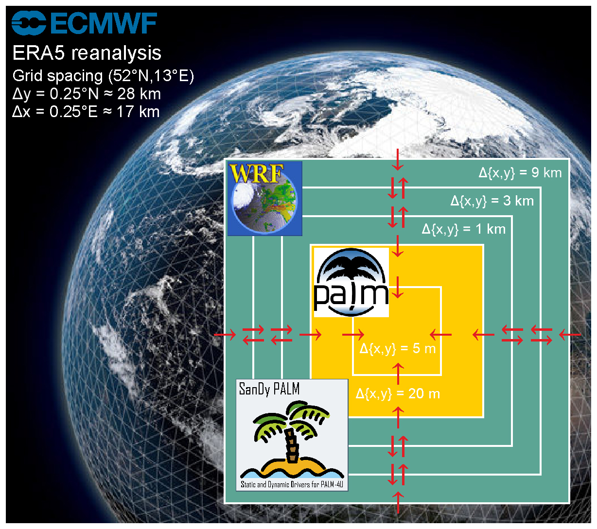
Figure 9 Nesting setup utilizing ERA5 for global boundary conditions, WRF for mesoscale forcing, and PALM as the microscale model.

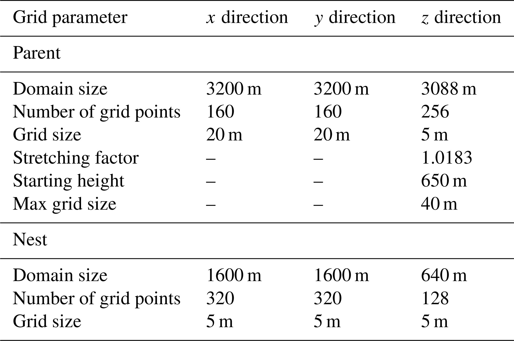
The nesting mode of the PALM internal grid nesting is set to one-way nesting, meaning the data are only transferred from the parent to the nest and the refined results from the nest are not transferred back to the parent. This is the recommended setting. The parent domain has a coarse horizontal grid size of dx=20 m by dy=20 m, and the nested domain has a finer grid size of dx=5 m by dy=5 m. The vertical grid size is dz=5 m in both cases; however, in the parent domain, we used vertical grid stretching. The stretching starts 10 m above the nested domain, which has a height of L_z=640 m. Since the urban boundary layer is approximately at a maximum height of 2045 m in our case, this means that the grid stretches throughout the boundary layer; however, the stretching is very gradual, using a small stretching factor of 1.0183. Although a uniform grid is recommended for large eddy simulation (LES), this grid has the advantages of a small vertical grid size at the surface, which allows for the evaluation of near-surface measurements, a uniform grid transition between the parent and nest near the surface, and a relatively small vertical grid cell count. Throughout the boundary layer, the vertical grid size increases gradually and reaches about dz=30 m at the maximum boundary layer height. In the upper damping layer above the urban boundary layer, the grid size further increases up to dz=40 m at the domain top at z=3088 m. The grid parameters are summarized in Table 2.

Table 2 Grid specifications in the PALM model for the parent domain (using vertical grid stretching) and the nested domain (without vertical grid stretching).

In the last third of the vertical height of the grid, starting at z=2050 m, we employed Rayleigh damping with a damping factor of 0.1. According to the PALM model documentation, this forces horizontal velocities, temperature, and humidity to their respective mean values provided by the mesoscale model. The damping is weak at the starting height and increases towards the top. The Rayleigh damping is intended to decrease gravity waves that might otherwise travel unhindered through the domain and be reflected at the top of the domain.

As the solver for the Poisson equation for perturbation pressure, we used the multigrid method with 2 iterations of the so-called W-cycle per time step and 2 iterations of the Gauss–Seidel method on each grid level. For the multigrid solver, the number of grid points needs to follow certain rules to achieve enough grid coarsening levels, and the performance of the solver is optimal when this number is 5 or higher. In our case, the grid of the parent domain allows for 5 coarsening levels, and the grid of the nested domain allows for 6 grid coarsening levels. In the case of parallel computing, these conditions need to hold for each partitioned subdomain.

In the urban surface model, the inner temperatures of walls, roofs, and windows are set to 298.15 K. To facilitate model spin-up and reduce atmospheric simulation spin-up time, we employed a wall/soil spin-up with a duration of 24 h and a time step of 10 s. In the OSM case, a smaller time step was necessary due to a metal surface type with high heat conductivity, which led to instabilities. The spin-up period corresponds to the 24 h interval from 18 July 2022 00:00 to 19 July 2022 00:00 (CEST), immediately preceding the simulation start time. The PALM model performs the wall/soil spin-up with a sinusoidal atmospheric temperature variation over time, specified by the mean and amplitude of daily temperature variation. The mean value ${\stackrel{\mathrm{‾}}{\mathit{\theta }}}_{\mathrm{spinup}}=\mathrm{299.15}\mathrm{K}$ and amplitude ${\stackrel{\mathrm{̃}}{\mathit{\theta }}}_{\mathrm{spinup}}=\mathrm{9.0}\mathrm{K}$ for atmospheric temperature during the wall/soil spin-up were approximately derived from mesoscale model results for the spin-up period.

For global radiation input, we used the “external” setting, where shortwave and longwave downwelling radiation are read from the dynamic driver. This approach has the advantage of considering clouds resolved by the mesoscale model in the radiation input. To resolve radiation within the urban canopy, the radiative transfer model is used in PALM. The radiation time step is set to 60 s. In the plant canopy model, the canopy drag coefficient is set to 0.2, and plant canopy transpiration is enabled. To create dynamic boundary conditions, the offline-nesting mode is used. To generate turbulence at the boundaries, the synthetic turbulence generator (Kadasch et al., 2021) is activated with an adjustment time step of 1800 s.

2.5 Measurement data

For the validation of the different PALM model simulation runs, we used measurement data from two different stations. The locations of the stations are illustrated in Fig. 1.

The first station is a weather monitoring tower situated in the garden of the Institute of Ecology at the Technical University of Berlin (TUB) on Rothenburgstraße (Fenner et al., 2014). The exact coordinates are 52.457232° N, 13.315827° E, and the terrain height is 46.5 m. The meteorological data generated by the tower are openly available on the website of the Urban Climate Observatory (UCO) (Scherer et al., 2024). This station is at the center of our inner nested PALM domain. From the many quantities available, we evaluated temperature, humidity, and wind. The available measurement heights are 2, 5, 10, 20, 30, and 40 m. However, wind speed and direction are only available at heights of 10 to 40 m, while humidity is only available at 2 and 5 m. For simplicity, we evaluated only the heights of 5 and 40 m for temperature, 5 m for humidity, and 10 and 40 m for wind speed.

The second station is the weather monitoring station “Dahlem” from the “Deutscher Wetterdienst” (DWD), which is located in the botanical garden in Berlin-Steglitz. The data were obtained from the DWD Open Data-Server (Deutscher Wetterdienst, 2024). The coordinates of this station are 52.4537° N, 13.3017° E, and the terrain height is 51 m. This location is only covered by our outer parent domain. The station features temperature and humidity measurements at a height of 2 m and wind speed measurements at a height of 36 m.

3 Results and discussion

In this study, we present a novel method for generating static and dynamic drivers for the PALM model, with an emphasis on static geographic data. Our results focus on two primary aspects: the impact of using various data sources to create static drivers and the subsequent effects on the PALM simulation outcomes. To achieve this, we compared the most relevant static-driver variables from our four approaches, both visually and statistically. Additionally, we evaluated how the use of different static drivers influences PALM simulations by running simulations for each case and comparing them against measurements and one another. This comparison is crucial for understanding the implications of data source selection for simulation accuracy and reliability.

3.1 Comparison of static drivers

Referencing Fig. 2, it is evident that the input data sources differ substantially in their representation of building footprints, vegetation, and pavement. We further investigate these variations in the final processed static drivers, focusing on the most significant variables. The static-driver variables are categorized into continuous and categorical types. For continuous variables, we examined terrain height (Fig. 10), building height (Fig. 11), tree height (Fig. 12), and leaf area index (LAI) (Fig. 13). For categorical variables, we evaluated building type (Fig. 14), vegetation type (Fig. 15), and pavement type (Fig. 16).

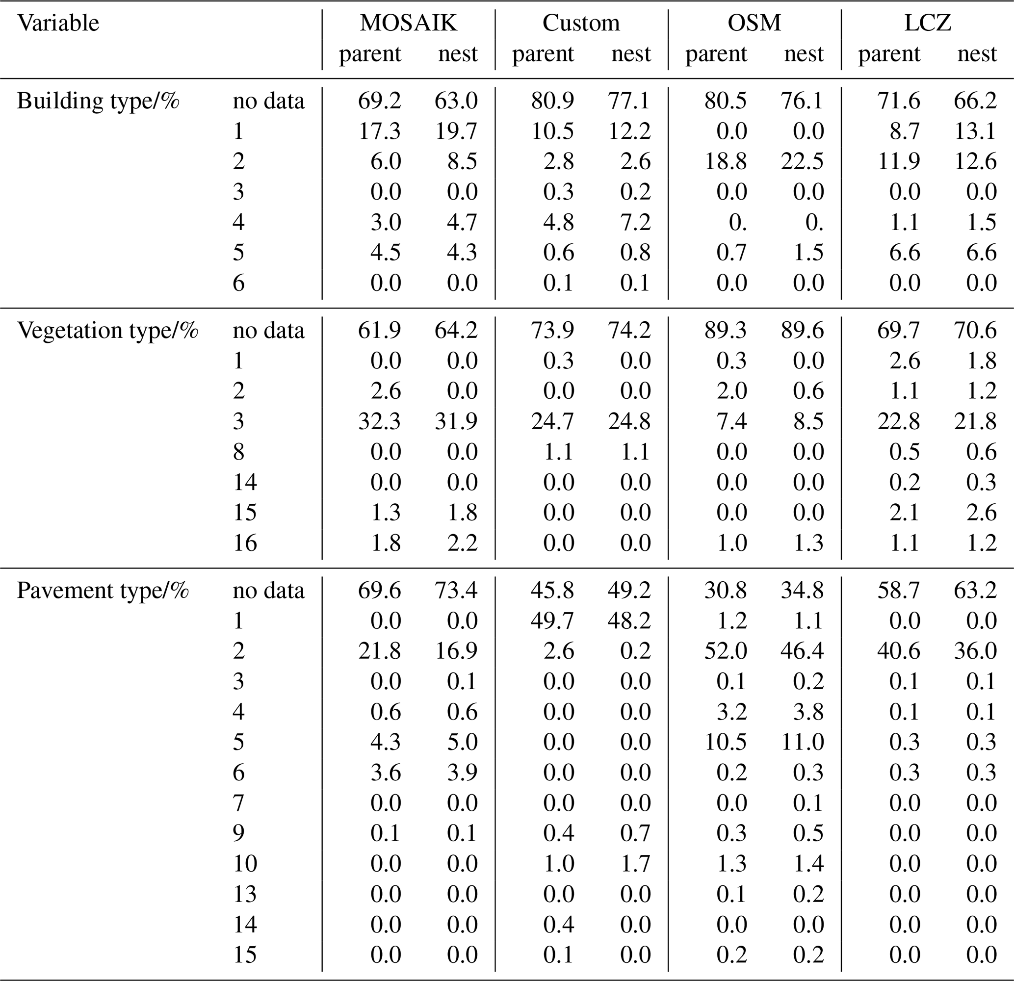
In addition to qualitative differences, a quantitative comparison containing several statistics was performed. For continuous variables, statistics (mean, standard deviation, minimum, and maximum) were calculated over the valid grid tiles only (excluding no-data values); the results are shown in Table 3. For categorical variables, the distribution of the observed types was calculated as a percentage of the total number of grid tiles (including no-data values); the results are given in Table 4. Types that do not occur are omitted in the table. To identify the valid types of a variable, we refer to the figure of the specific type for a legend connecting the type number to a text description. The table also lists no-data values to compare the number of grid cells lacking specific types. Calculations were performed separately for parent and nested domains.

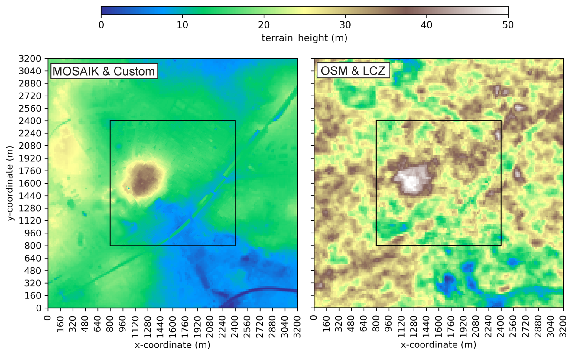
Figure 10 Comparison of terrain height for the different static drivers.

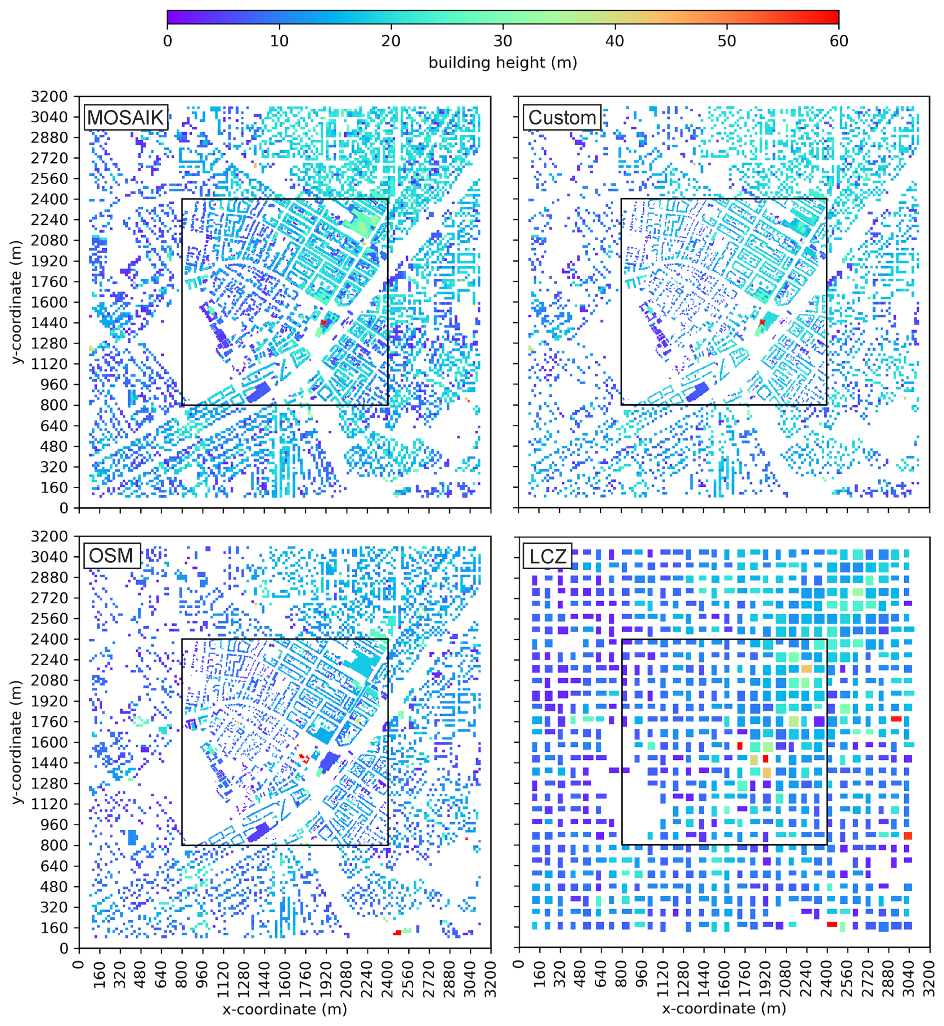
Figure 11 Comparison of building height for the different static drivers.

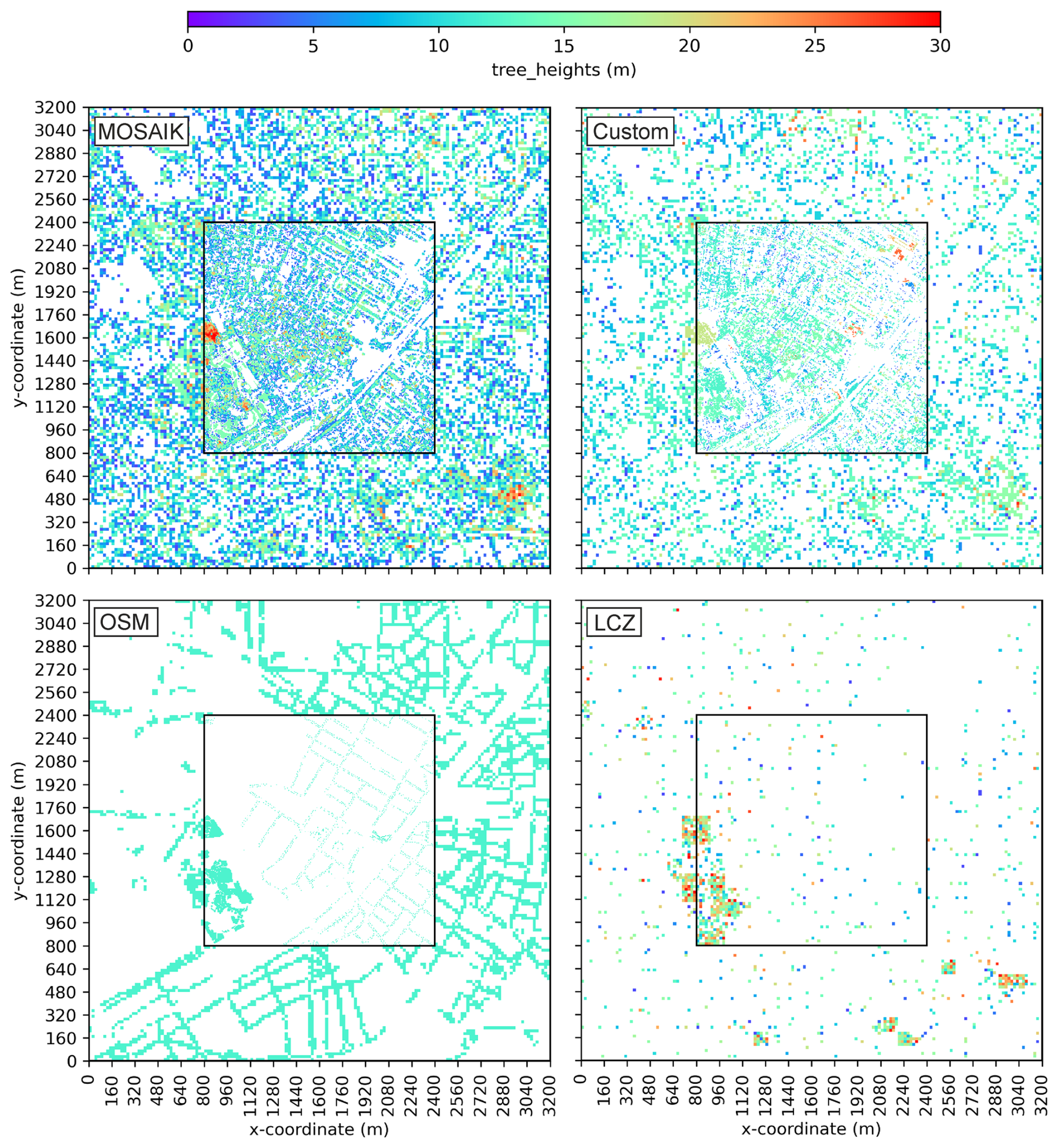
Figure 12 Comparison of tree height for the different static drivers.

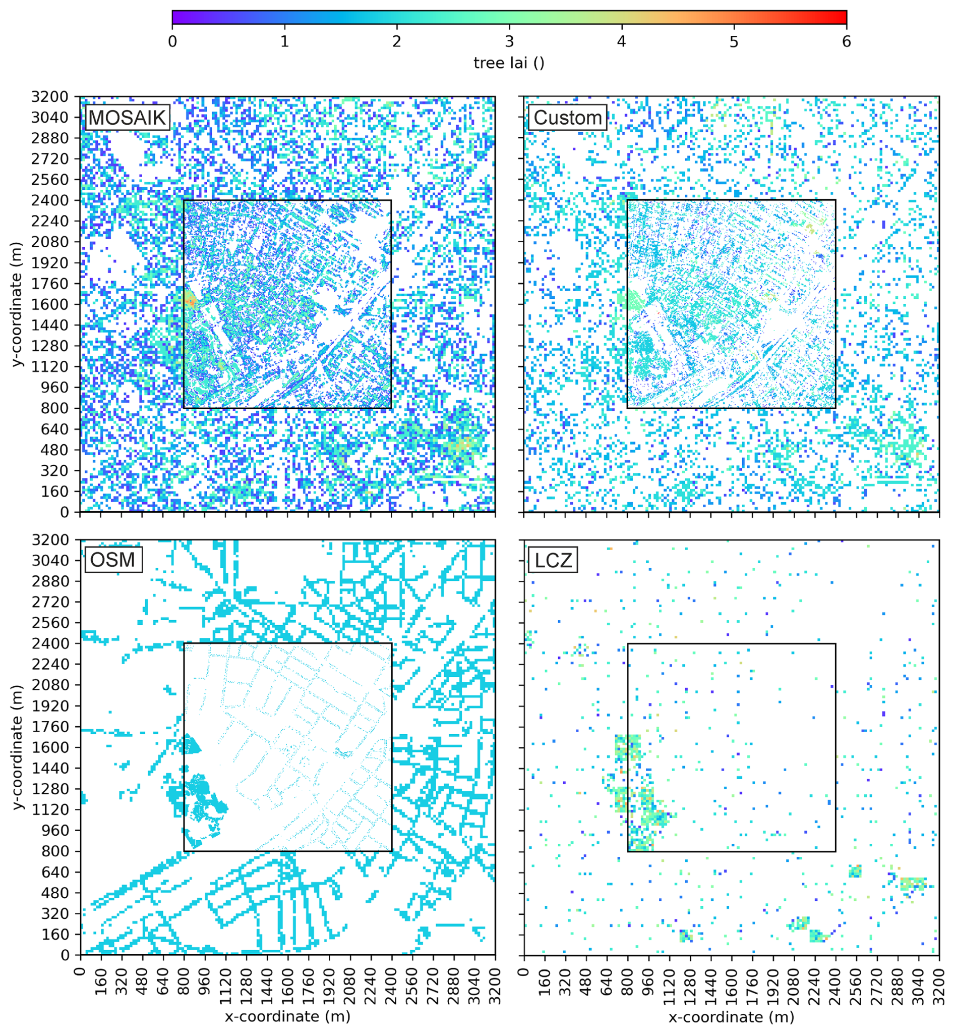
Figure 13 Comparison of leaf area index (LAI) for the different static drivers.

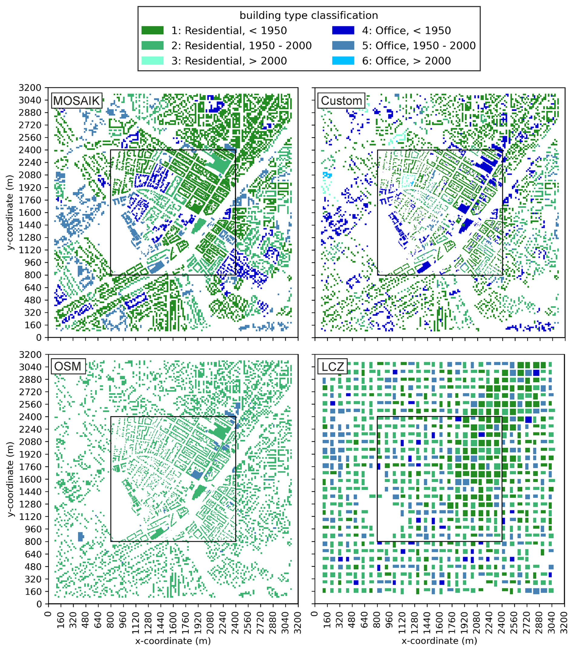
Figure 14 Comparison of building type for the different static drivers.

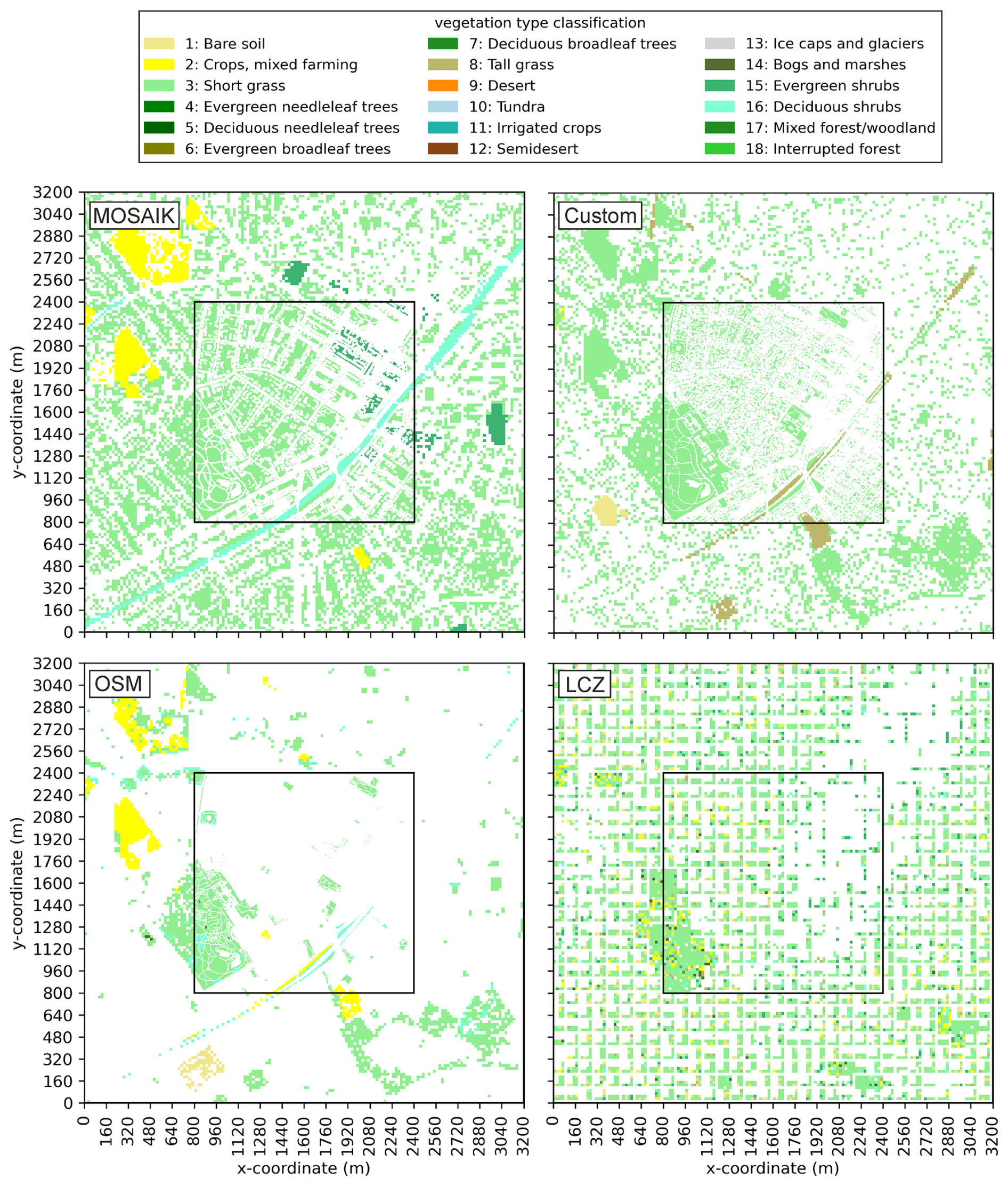
Figure 15 Comparison of vegetation type for the different static drivers.

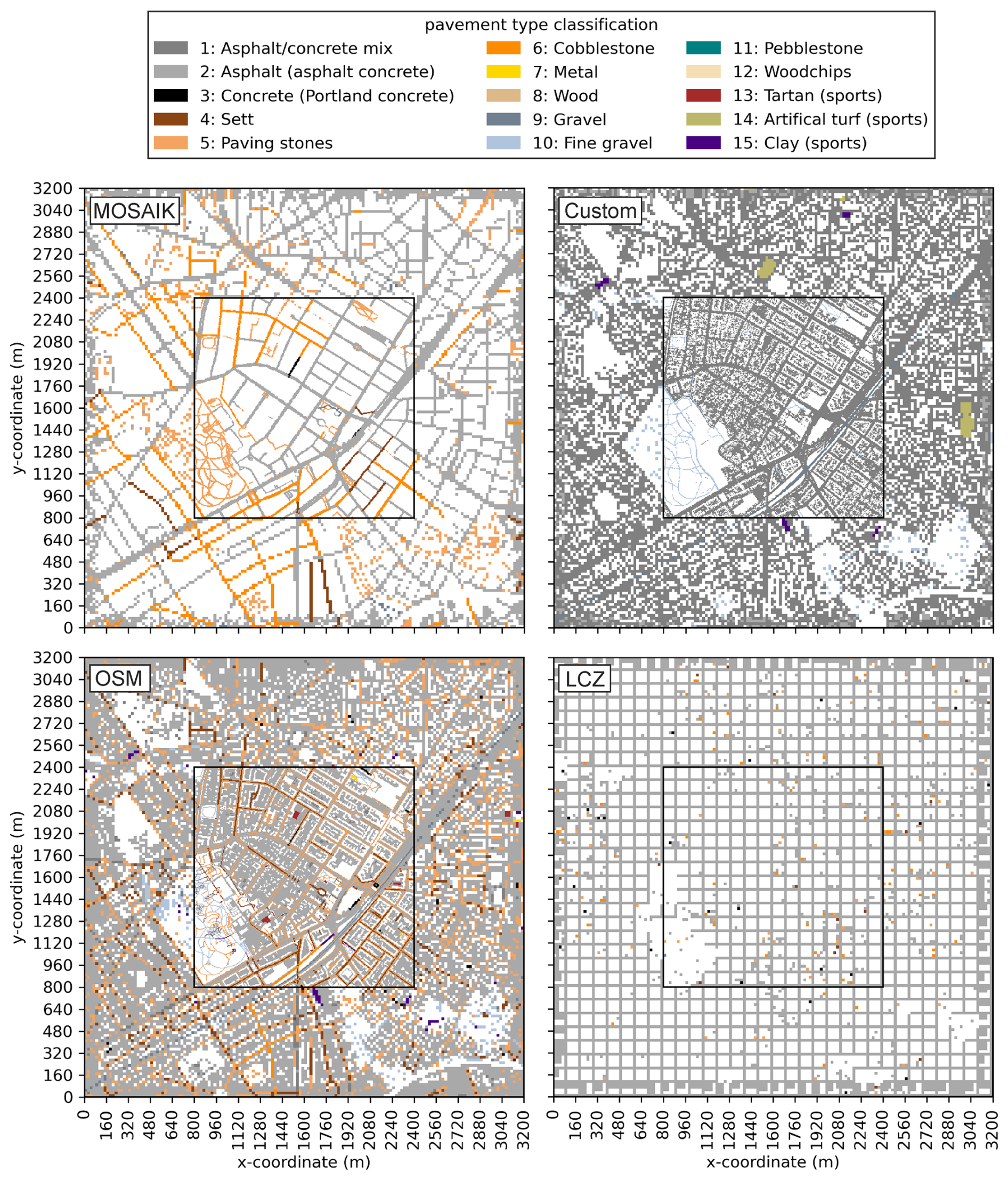
Figure 16 Comparison of pavement type for the different static drivers.

Table 3 Comparison of static drivers showing the statistics mean, standard deviation (std), minimum, and maximum for the continuous variables terrain height, building height, tree height, and tree LAI.

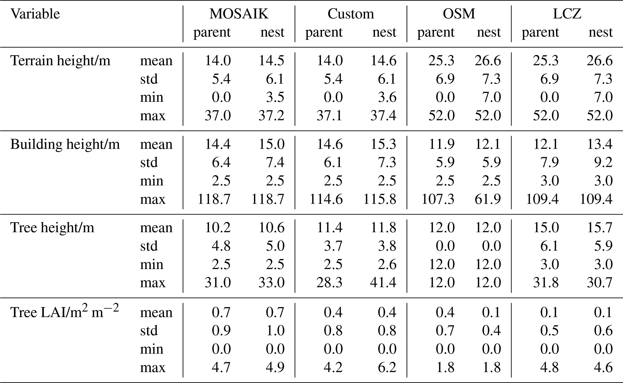
Table 4 Comparison of static drivers showing the percentage distribution of observed types for the categorical variables building type, vegetation type, and pavement type.

For terrain height, shown in Fig. 10, despite the four cases, there are only two main data sources: the terrain height for MOSAIK and Custom originates from municipal data, while OSM and LCZ utilize a remotely sensed digital elevation model (DEM). The MOSAIK terrain height was slightly post-processed, resulting in negligible differences from the municipal terrain height. The terrain height presented here is relative to the origin of the z coordinate (origin_z) of the parent domain, with origin_z≈32 m for MOSAIK and Custom and origin_z≈26 m for OSM and LCZ. The remotely sensed DEMs (OSM and LCZ) exhibit higher average and maximum values compared to the municipal DEMs (MOSAIK and Custom). Additionally, the remote sensing DEMs (OSM and LCZ) have a larger range of values, are generally noisier, and lack the detail found in the municipal DEMs (MOSAIK and Custom).

Regarding building height, shown in Fig. 11, the MOSAIK data show larger building footprints compared to the Custom and OSM cases. All three datasets struggle to resolve building footprints at the coarser scale of the parent domain. The LCZ method does not accurately capture the exact building footprints at either scale but maintains consistency across them. Building heights are similar in MOSAIK and Custom, while OSM and LCZ exhibit comparable heights. OSM combines available heights with WSF3D data, which can result in occasional anomalies due to gaps filled by WSF3D data. In contrast, LCZ relies solely on WSF3D, leading to more consistent building heights.

Tree heights vary significantly across the datasets; see Fig. 12. MOSAIK features extensive tree cover, while Custom has fewer trees. OSM includes only individual trees with no tree patches, and LCZ shows sparse tree coverage. Generally, tree heights in MOSAIK are larger than those in Custom, although there are regions where the reverse is true. OSM lacks specific tree height data, so default constant heights were used. In contrast, LCZ tree heights align with those in MOSAIK, as their distribution was derived from the same data source.

For the tree leaf area index (LAI), which is shown in Fig. 13, the MOSAIK, Custom, and LCZ cases exhibit similar values due to the LAI limiting process during SanDyPALM processing. The original LAI values in MOSAIK were significantly higher, requiring moderation to prevent excessive humidity spikes near vegetation. The variation in LAI for Custom arises from height-dependent default calculations. In contrast, OSM shows no variation in tree LAI; due to the absence of values for both tree LAI and tree height, constant default values are assumed for both.

Building types across the datasets show notable variations, as can be seen in Fig. 14. Predominantly, buildings are classified as types 1, 2, 4, and 5 (residential and office before 2000), with types 3 and 6 (residential and office after 2000) being rare. The Custom data, sourced directly from the municipality, emphasizes type 1 (residential before 1950) and type 4 (office before 1950), while types 2 and 5 are less common. In contrast, the MOSAIK data, also based on municipal sources but further post-processed, show a significantly higher occurrence of type 5 compared to Custom, nearly matching type 4. Occasionally, buildings classified as office in MOSAIK are categorized as residential in Custom, and vice versa. OSM data predominantly feature residential buildings, while LCZ data closely resemble MOSAIK data, as their type probabilities were derived from them. Overall, building type classifications exhibit significant variability across the different approaches.

Vegetation types – see Fig. 15 – have distinct variations across the datasets as well. The highest vegetation amount is in the MOSAIK case, followed by LCZ and Custom, with OSM data having the sparsest vegetation. The dominant type across all cases is type 3 (short grass). The LCZ case also includes significant amounts of type 1 (bare soil) and type 2 (crops), while MOSAIK only includes type 2 (crops) in the parent domain. The type distribution for LCZ was derived from MOSAIK data for the entire city boundary of Berlin, explaining the distribution differences. In the OSM case, a small amount of type 1 (bare soil) and a significant amount of type 2 (crops) are found in the parent domain. Both Custom and LCZ contain some type 8 (tall grass). A similar amount of type 15 (evergreen shrubs) is found in both MOSAIK and LCZ, while type 16 (deciduous shrubs) is present in MOSAIK, OSM, and LCZ but absent in Custom. Overall, the amount and distribution of vegetation vary significantly among the four cases.

Pavement type, as shown in Fig. 16, varies as well significantly across the datasets. MOSAIK has sparse pavement coverage (26.6 %–30.4 %), while Custom (50.8 %–54.2 %) and OSM (65.2 %–69.2 %) likely overestimate pavement. LCZ falls in between (36.8 %–41.3 %) but remains higher than MOSAIK. The dominant pavement types differ: type 2 is prevalent in MOSAIK, OSM, and LCZ, while type 1 is dominant in Custom. MOSAIK includes significant amounts of types 5 and 6 (paving stones and cobblestone), OSM shows types 4 and 5 (sett and paving stones), and both Custom and OSM contain some type 10 (fine gravel). Only OSM includes type 7 (metal), which caused issues during the PALM wall/soil spin-up due to high heat conductivity and was resolved using a smaller time step. Other types are sparse. Overall, the amount and type of pavement vary significantly among the cases.

We found that the MOSAIK case tends to overestimate building footprints and vegetation, while the OSM and Custom cases generally underestimate vegetation. The overestimation in MOSAIK likely results from the “all-touched” rasterization technique, which rasters all grid tiles touched by a vector polygon. Additionally, MOSAIK data may have been post-processed to prioritize vegetation over pavement. In contrast, the Custom and OSM cases raster only those grid tiles whose centers are covered by a vector polygon, resulting in more realistic building footprints. However, a downside of the Custom and OSM cases is that the vegetation appears too sparse, and LAI data are missing, necessitating the use of default values. The overestimation of pavement in these cases occurs because, with sparse vegetation, pavement becomes the default surface type when no other type is defined. While MOSAIK data have been post-processed and prioritized, the other data sources are relatively raw. During processing in SanDyPALM, consistency checks and corrections were uniformly applied across all datasets, although customized strategies might have benefited different datasets.

This analysis illustrates that the choice of data source significantly influences outputs, with each processing strategy presenting its own advantages and disadvantages. Overall, the key differences between the test cases highlight variations in urban morphology, vegetation coverage, and data completeness, all of which may impact the outcomes of PALM simulations.

3.2 Comparison of PALM results to measurements

The next step in our investigation involved simulating the same test case using the four different static drivers, while keeping the dynamic driver consistent. The dynamic driver is created using the same mesoscale data, but it may still vary slightly among the cases because the surface layer model used to fill the near-surface data gaps in the mesoscale input data depends on roughness properties derived from the static driver. This approach allowed for a comparison of the PALM results, along with the WRF results, against measurements from the TUB monitoring tower located within the inner nested domain and the DWD weather station, which is covered only by the parent domain. The comparison metrics used in this study are the mean bias error (MBE) and the root mean square error (RMSE).

3.2.1 Tower measurements

For our investigation, we selected a limited number of measurement heights from the tower. For example, measurements at 2 and 5 m are not expected to differ significantly, particularly in numerical models where values are interpolated from sparse data points near the surface. Air temperature T was evaluated at heights of 5 and 40 m above ground level (a.g.l.), relative humidity ϕ_rel at 5 m, and horizontal wind speed U_h at 10 and 40 m. The comparison of WRF and PALM results with the tower measurements is presented in Fig. 17, and the metrics for all models compared to the tower data are compiled in Table 5.

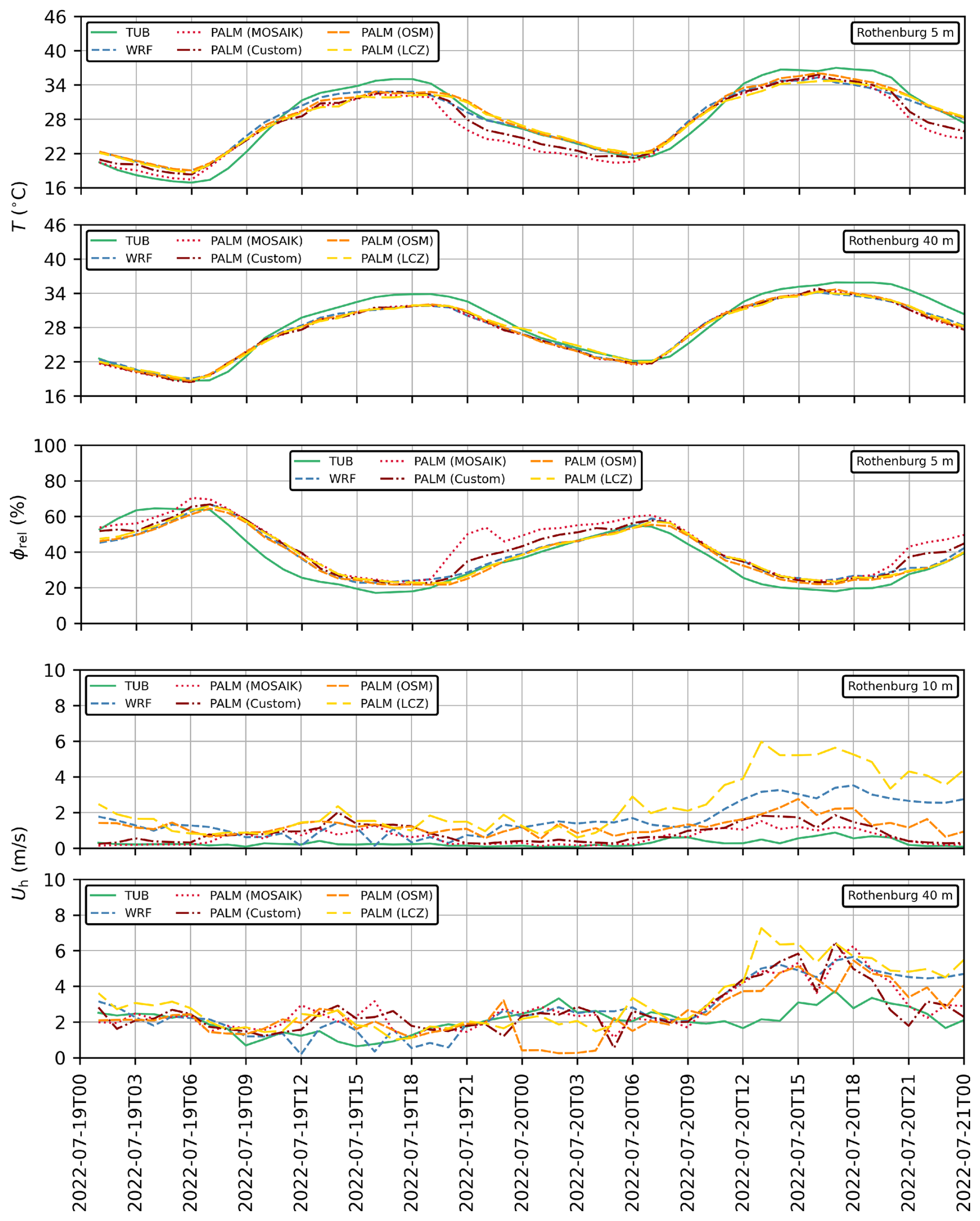
Figure 17 Comparison of WRF and PALM results of temperature T, relative humidity ϕ_rel, and horizontal wind speed U_h against measurements from the TUB tower at “Rothenburgstraße” (located in the nested domain).

Table 5 Metrics for comparing WRF and the PALM results with measurements from the TUB Tower “Rothenburgstraße” (located in the nested domain).

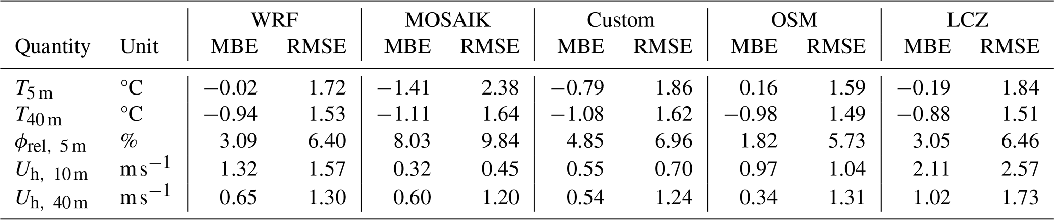
The general agreement between WRF and PALM results and the measurements indicates that all relevant physical processes are well resolved. However, some notable deviations exist. For temperature at 40 m, WRF and all PALM results are nearly identical, but all show lower daytime temperatures compared to tower measurements. At 10 m, the PALM models using MOSAIK and Custom data deviate increasingly from the WRF model, while the OSM and LCZ models remain close to WRF. Unfortunately, this deviation is away from the measurements and is likely related to humidity.

The 5 m relative humidity shows increased nighttime values between sunset and sunrise, particularly for the PALM models using MOSAIK and Custom static drivers. The main difference is that these static drivers feature significantly more vegetation than the others. The observed higher humidity may result from a combination of evapotranspiration from soil and vegetation, reduced atmospheric mixing, and dew formation. Even after sunset, plants continue to release water vapor through transpiration, while moisture retained by soil and vegetation during the day can evaporate as temperatures drop. Additionally, surface cooling can create a stable atmospheric layer near the ground, reducing vertical mixing and allowing the air close to the surface to retain more moisture. Dew formation and subsequent evaporation can also contribute to localized increases in humidity.

These combined factors could explain the high humidity levels observed in vegetated areas during the evening and why these effects are more pronounced with MOSAIK or Custom data, which feature greater vegetation coverage. However, it remains unclear whether the amount of vegetation is overestimated in the input data or if the described effects are exaggerated in the PALM model.

The measured wind speeds during this period are generally low. At 40 m, WRF slightly overestimates wind speed compared to tower measurements, while the PALM models generally follow WRF, showing deviations towards both stronger and weaker wind speeds. At 10 m, the PALM models tend to output lower wind speeds than WRF, aligning better with the measurements, except for the LCZ case, which records significantly higher wind speeds on the second day. The LCZ case is unique, as the buildings are not accurately resolved, and the arrangement near the tower may differ significantly from the actual courtyard of the TUB tower.

Additionally, the generally low measured wind speeds and the tendency for simulations to overestimate wind speed can be attributed to the courtyard's surroundings, which are lined with tall, dense trees. This creates significant wind shading, an effect not accounted for by the WRF model. The accuracy of the PALM models in this location also heavily relies on the precise locations and characteristics of the trees and buildings.

3.2.2 Station measurements

WRF and PALM results were compared to measurements from the DWD station in Dahlem, which is only resolved in the parent domain of our PALM setup. Air temperature T and relative humidity ϕ_rel were evaluated at a height of 2 m a.g.l., while horizontal wind speed U_h was evaluated at 36 m. These evaluation heights correspond to the measurement heights of the station. In the PALM simulation results, the temperature and humidity were approximately evaluated at the first grid point above ground at a height of 2.5 m; the wind speed was vertically interpolated from the neighboring grid points to the exact measurement height. The comparison of WRF and PALM results with the station measurements is presented in Fig. 18, and the metrics for all models compared to the station data are compiled in Table 6.

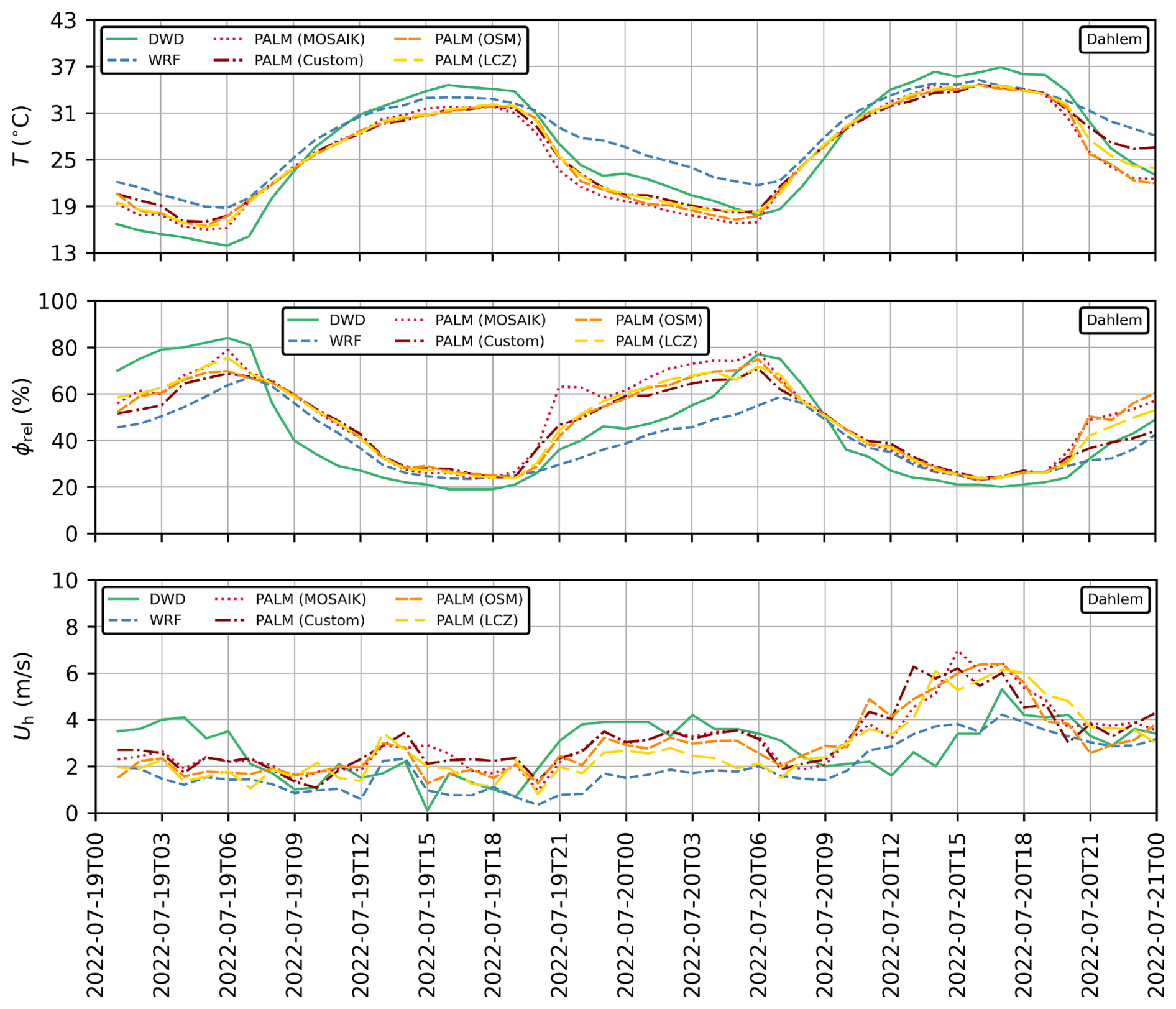
Figure 18 Comparison of WRF and PALM results for temperature T, relative humidity ϕ_rel, and horizontal wind speed U_h against measurements from the DWD station “Dahlem” (located in the parent domain).

Table 6 Metrics for comparing WRF and PALM results from the four test cases with measurements from the DWD station “Dahlem” (located in the parent domain).

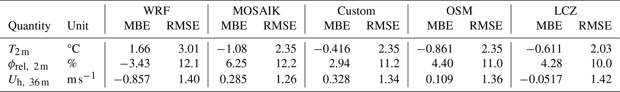
For this station, the WRF model overestimates nighttime temperatures, likely due to an exaggerated urban heat island effect. The LCZ map used in WRF classifies the area around the station as “LCZ 6” (open low-rise), which is appropriate for the entire 1 km WRF grid tile but does not accurately represent the densely vegetated botanical garden around this station. In contrast, the PALM models, which realistically resolve buildings and vegetation, are significantly closer to the measurements in this case.

Humidity is underestimated by WRF at night and overestimated during the day. The PALM models generally predict higher humidity than WRF, with a moderate increase during the day and a more pronounced rise at night. At the end of the first night, PALM results align more closely with measurements than WRF, but on the second night and early on the third night, they overestimate humidity compared to the measurements. Similarly to the tower data, PALM humidity shows significant spikes around sunset.

Wind speed at this location is comparable to that at the upper tower location, which has a similar height. While WRF overestimates wind speed at the tower, it underestimates it at the station. This discrepancy may arise because the tower is surrounded by large trees and buildings that create wind shading, whereas the station is situated in an open park with less restricted wind flow. The WRF model, lacking detailed information about trees and buildings, resolves both locations similarly. In contrast, wind speeds from the PALM models are closer to the measurements, with all PALM models performing comparably well.

3.3 Comparison of PALM results to each other

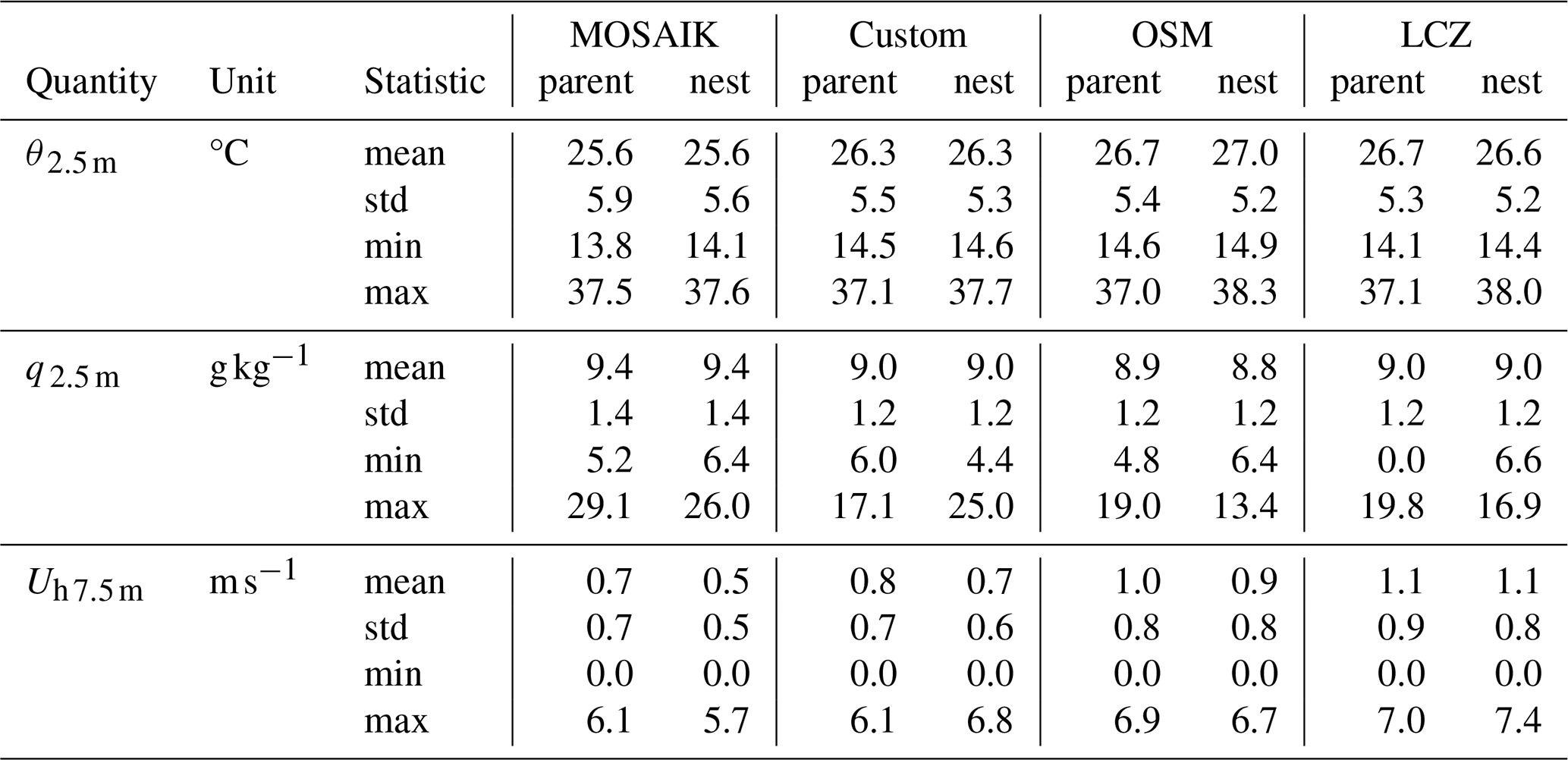
To compare the PALM simulation results across the four test cases, we evaluated the potential temperature θ (Fig. 19) and the mixing ratio q (Fig. 20) at the first vertical centered grid level, corresponding to a height above ground of h_AGL=2.5 m. The horizontal wind speed U_h (Fig. 21) was evaluated at the second vertical centered grid level, corresponding to a height of h_AGL=7.5 m. All quantities were time-averaged over the entire simulation period, which spanned 2 d. A quantitative comparison of the statistics for the four different simulation test cases is presented in Table 7. For each quantity, the mean, standard deviation (std), minimum (min), and maximum (max) values were calculated over the entire 2 d simulation period and across all grid points (excluding no-data values).

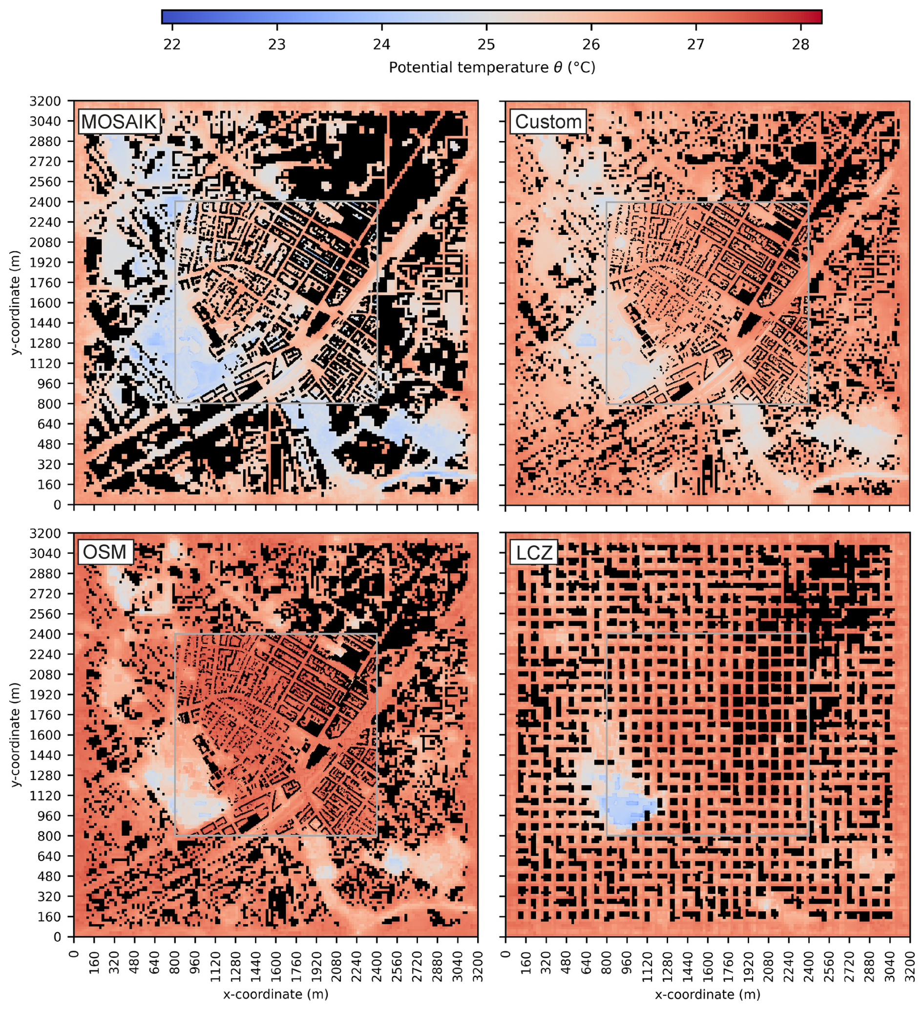
Figure 19 Comparison of time-averaged potential temperature θ evaluated at h_AGL=2.5 m.

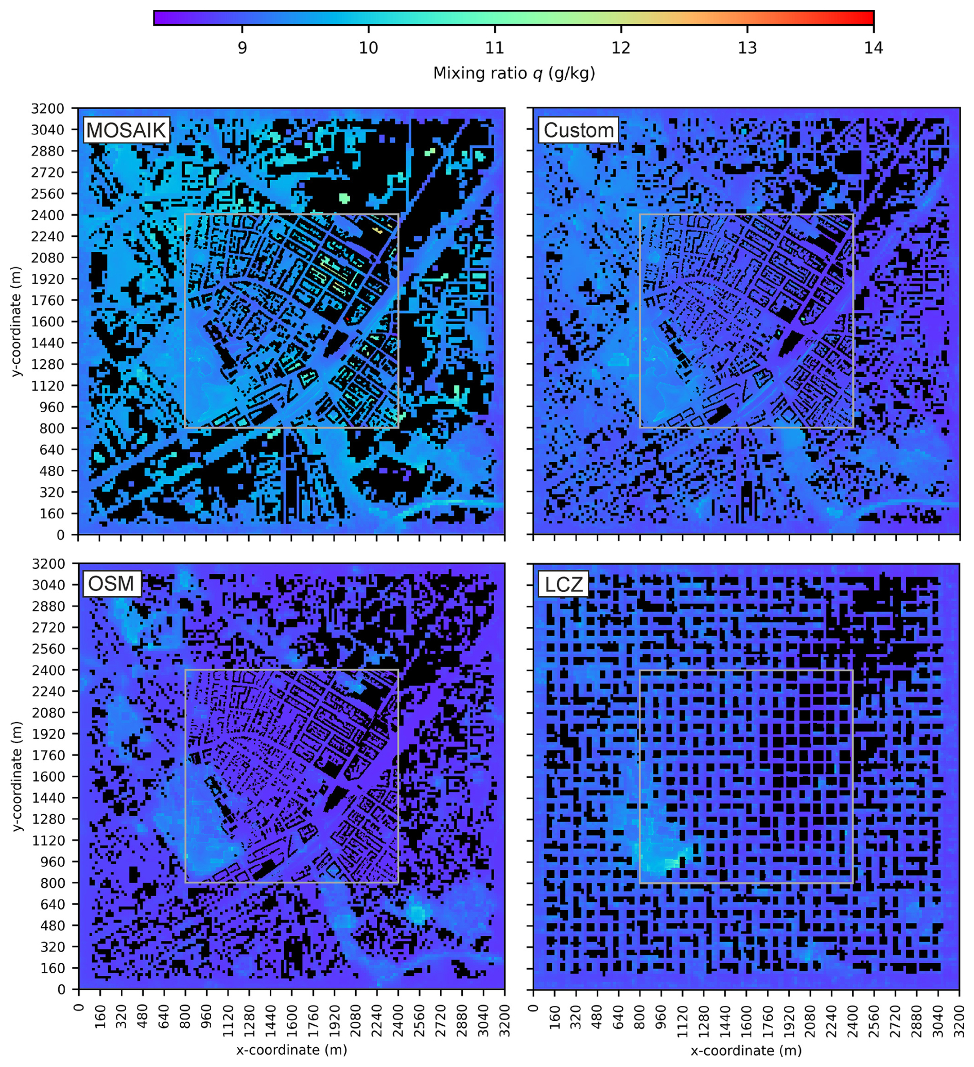
Figure 20 Comparison of time-averaged mixing ratio q evaluated at h_AGL=2.5 m.

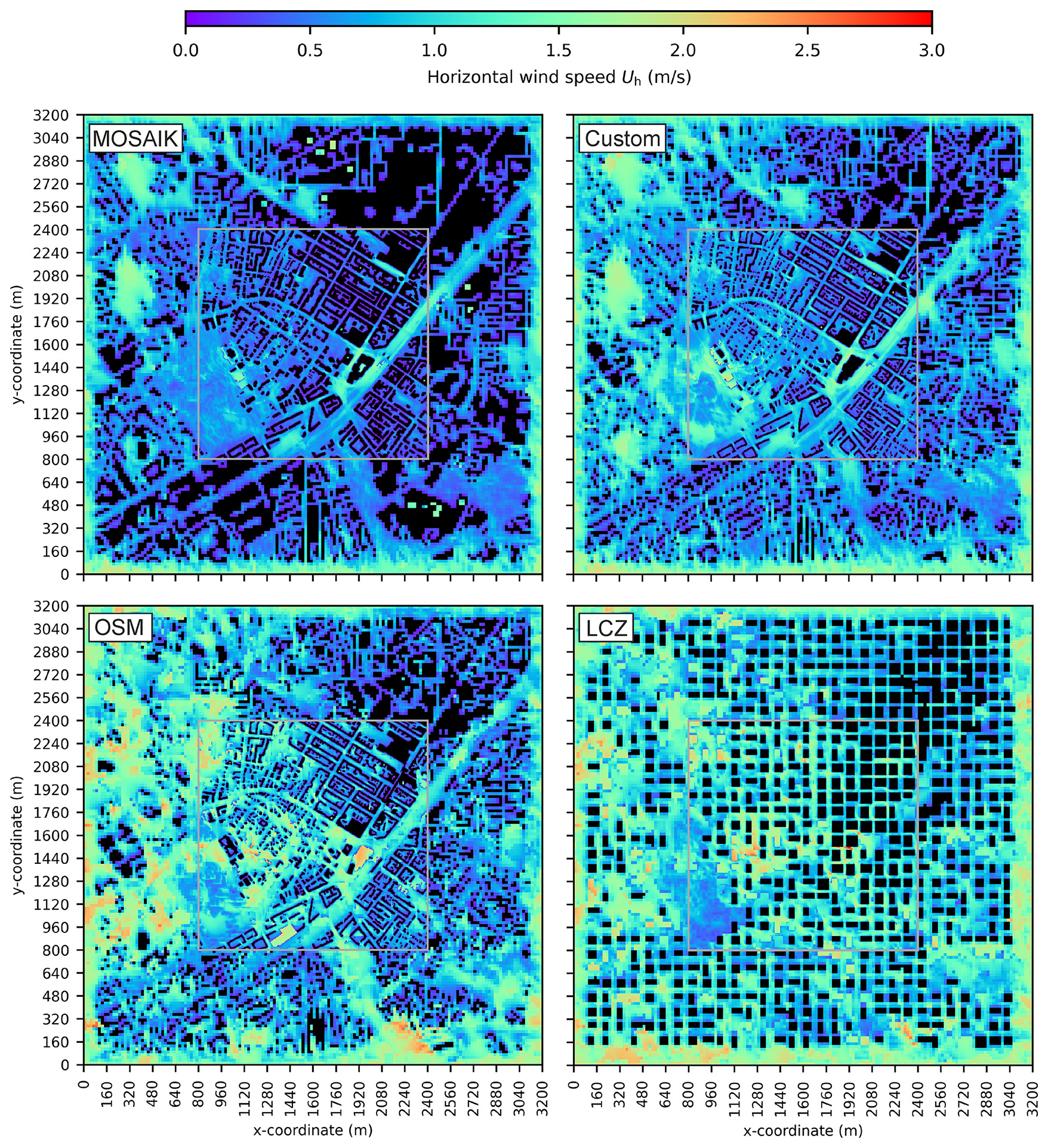
Figure 21 Comparison of time-averaged horizontal wind speed U_h evaluated at h_AGL=7.5 m.

Table 7 PALM result statistics for the four different test cases.

One issue we encountered, particularly when applying the LCZ method to the parent grid at a coarse resolution of 20 m, is the gap filling of terrain and building grid boxes performed by PALM. While this gap filling is an important preprocessing step for the PALM model, it prevents us from using the exact building shapes we designed. We observed that narrow street canyons became blocked, rectangular footprints were altered into arbitrary shapes, and small courtyards formed within building areas. The source of this problem is that street canyons that are only one grid box wide are considered too narrow by the PALM model. Conversely, we cannot use additional grid boxes at coarse resolutions, as this would result in excessively wide street canyons. Our intention in creating the LCZ4PALM method was to design regularly shaped buildings at coarse resolutions and to prevent the usual clustering of dense building areas into one continuous mass. However, running the model at such coarse resolutions remains challenging, and we must accept that, in the simulation, the buildings and street canyons do not take the shapes we intended.

In our investigation of temperature, humidity, and wind speed, we observed notable differences among the test cases. First, examining mean temperatures in the nested domain in Fig. 19, we find 25.6 °C for MOSAIK, 26.3 °C for Custom, 27.0 °C for OSM, and 26.6 °C for LCZ. There is a clear increase in temperature from MOSAIK to Custom to LCZ to OSM. We suspect the reason for this is mainly due to differences in vegetation because the amount of vegetation approximately follows the inverse order, with MOSAIK having the highest and OSM the lowest amount. The temperatures in the parent domain behave similarly: the mean temperatures are lowest in MOSAIK, second in Custom, and third in OSM and LCZ with the same value. The minimum and maximum temperatures exhibit more variability between the parent and nested domains.

The humidity, which is shown in Fig. 20, has the largest divergence among the test cases and between the nested and parent domains. The mean humidity is particularly high in the MOSAIK case at 9.4 g kg⁻¹, compared to the other cases, which range from 8.8 to 9.0 g kg⁻¹. This is likely due to the higher vegetation density in the input data. MOSAIK also produces extreme maximum humidity values of up to 29.1 g kg⁻¹, which seem unrealistic. Conversely, the LCZ case exhibits extremely low values, down to 0.0 g kg⁻¹. However, such physically unrealistic values were observed only in rare instances in space and time. Their occurrence was limited to only one or two output time steps at sunrise or sundown and only a few grid boxes in narrow street canyons or courtyards, particularly in conjunction with an abundance or absence of vegetation nearby. For example, the low humidity in the LCZ case occurred only in one output time step and in a single grid box that has a paved surface beneath and is surrounded by tall buildings. Although it is advisable to avoid narrow street canyons or courtyards, preventing them in practical workflows is challenging, especially at relatively coarse resolutions.

Finally, the wind speed (Fig. 21) is generally lowest in the MOSAIK case, followed by Custom, OSM, and LCZ. This trend may again be attributed to vegetation density, which is highest in MOSAIK and lower in OSM and LCZ. Additionally, the OSM and LCZ cases partially or fully utilize approximate building heights derived from coarse global datasets, and their terrain elevation data are less accurate compared to the more precise representations in MOSAIK and Custom.

Interestingly, the OSM and LCZ test cases, despite being automatically generated and using approximations, yield results comparable to the heavily preprocessed MOSAIK and Custom cases. In the LCZ case, while the local distribution is less realistic due to unresolved buildings and streets, areas like the botanical garden in the lower left of the nested domain are well represented. Despite geographic-precision shortcomings, the overall results of the LCZ case compare surprisingly well to the other cases.

The main question remains: which dataset most accurately represents the selected district, and how can we further improve data quality? Each test case has its advantages and disadvantages. The MOSAIK case utilized extensive data and underwent significant preprocessing, yet it overestimates building footprints and underpredicts temperature, suggesting an excessive amount of vegetation or that PALM overestimates vegetation impact. The Custom case, designed by an expert, benefits from more accurate building footprints and less vegetation cover, leading to reduced temperature underprediction near the surface. The OSM case, fully automatically processed, features similar building footprints to the Custom case but significantly less vegetation, resulting in the highest overall temperatures. Wind speeds are also higher than in the MOSAIK and Custom cases, likely due to differences in vegetation, building heights, and terrain elevation. Finally, the LCZ case, also automatically processed, shows relatively high temperatures and the highest wind speeds, with variations in building heights, footprints, and distribution impacting both temperature and wind speed results. Similarly to the OSM case, differences in terrain elevation and vegetation density also play a role.

Overall, this research indicates that the outcomes of realistic urban microclimate simulations clearly depend on input data. Different data sources for the same test case can yield varying results. However, the outputs do not diverge excessively, especially when considering that the set of test cases – including OSM and LCZ data sources – can be seen as quite diverse. The overall features of the microclimate simulations are similar, with no extreme outliers in the comparison statistics, except for the described instabilities regarding humidity in certain locations.

4 Conclusions

In this study, we presented SanDyPALM, an innovative toolkit designed to streamline the creation of static and dynamic input data for the PALM model, thereby enhancing realistic microclimate simulations. The main motivation of this toolkit was to make the preparation of input data faster and more user-friendly. This was achieved by combining static and dynamic-driver generation into one package and also by introducing methods for automatic generation of static input data.

We introduced two novel methods, OSM2PALM and LCZ4PALM, which facilitate the generation of static drivers from widely available geospatial data sources. These methods enhance the accessibility and applicability of urban climate modeling, allowing for parametric studies and the creation of models anywhere on the earth. LCZ4PALM is especially useful for creating an approximate model on coarse grids, where real building shapes cannot be resolved, while OSM2PALM creates an accurate urban model resolving buildings and vegetation to the degree available in the database.

By comparing four static drivers derived from different sources – MOSAIK, Custom, OSM, and LCZ – we observed substantial variations in the representation of building footprints, vegetation, and pavement. The MOSAIK dataset, while rich in detail, tended to overestimate building footprints and vegetation, whereas the Custom, OSM, and LCZ datasets underestimated vegetation coverage.

The results of our simulations were validated against measurements from a weather monitoring tower and a weather station, revealing that all models captured the essential physical processes. However, notable discrepancies were observed, particularly in temperature and humidity. The PALM models using MOSAIK and Custom data exhibited elevated nighttime humidity levels, likely due to their greater vegetation density. In contrast, the OSM and LCZ models, despite being based on approximations, produced results closer to measurements due to their lower vegetation density. This raises the question of whether the observed deviations stem from the amount of vegetation or the modeling approach used in PALM.

In very rare cases, unrealistic humidity values were observed inside narrow street canyons or courtyards for a limited number of output time steps. To address this issue, either the static input data need to be adjusted or the humidity model in PALM needs to be refined to limit humidity to realistic values. Another challenge is that the urban morphology is altered by PALM preprocessing to fill narrow street canyons and terrain, which modifies building shapes and closes off a substantial number of street canyons. Without changes to the PALM model itself, it may be advisable to apply further terrain smoothing, enforce wider street canyons, or increase the grid resolution of the parent domain.

The results indicated that expert-driven approaches, such as the MOSAIK and Custom datasets, provide the more detailed and accurate representations of urban environments. But the automated methods OSM2PALM and LCZ4PALM, while lacking detail, can yield comparably accurate results. Therefore, they offer a viable alternative when expert resources are limited. As a result, the required level of detail needed to obtain realistic meteorological quantities from urban microclimate simulations is lower than expected. However, to get the highest-precision results, it is still necessary for an expert to thoroughly prepare the input data.

Future research can focus on refining these automated tools, exploring additional data sources to further enhance the reliability of urban microclimate simulations and performing additional investigations on the role of static input data: (1) terrain smoothing could be useful, especially when using the LCZ method, to prevent the necessity for excessive gap filling by the PALM model. (2) The LCZ method was used with data specifically generated for the city of Berlin and needs to be extended to other cities to be able to generalize. (3) The dynamic-driver tool could be adjusted to accept other input data sources besides WRF. (4) Additional open data sources could be implemented, especially for tree height and LAI, because these are lacking in OSM and LCZ data sources. (5) An interesting application of the OSM2PALM and LCZ4PALM methods would be to combine them in the following way: a large and low-resolution parent domain is based on LCZ and driven by a mesoscale model, while a high-resolution nested domain is based on a detailed OSM model. This approach based solely on open data would leverage the advantages of both methods, providing a low-detail model at coarse resolution and a high-detail model at fine resolution. (6) Further investigations are necessary about the impact of static input data on mitigation strategies for climate change or urban heating. (7) The issue of extreme humidity values requires further investigation – specifically, by further analyzing the impact of static input data and examining how water content is managed in PALM.