HIDRA3: a deep-learning model for multipoint ensemble sea level forecasting in the presence of tide gauge sensor failures

Accurate modeling of sea level and storm surge dynamics with several days of temporal horizons is essential for effective coastal flood responses and the protection of coastal communities and economies. The classical approach to this challenge involves computationally intensive ocean models that typically calculate sea levels relative to the geoid, which must then be correlated with local tide gauge observations of sea surface height (SSH). A recently proposed deep-learning model, HIDRA2 (HIgh-performance Deep tidal Residual estimation method using Atmospheric data, version 2), avoids numerical simulations while delivering competitive forecasts. Its forecast accuracy depends on the availability of a sufficiently long history of recorded SSH observations used in training. This makes HIDRA2 less reliable for locations with less abundant SSH training data. Furthermore, since the inference requires immediate past SSH measurements as input, forecasts cannot be made during temporary tide gauge failures. We address the aforementioned issues using a new architecture, HIDRA3, that considers observations from multiple locations, shares the geophysical encoder across the locations, and constructs a joint latent state that is decoded into forecasts at individual locations. The new architecture brings several benefits: (i) it improves training at locations with scarce historical SSH data, (ii) it enables predictions even at locations with sensor failures, and (iii) it reliably estimates prediction uncertainties. HIDRA3 is evaluated by jointly training on 11 tide gauge locations along the Adriatic. Results show that HIDRA3 outperforms HIDRA2 and the Mediterranean basin Nucleus for European Modelling of the Ocean (NEMO) setup of the Copernicus Marine Environment Monitoring Service (CMEMS) by ∼ 15 % and ∼ 13 % mean absolute error (MAE) reductions at high SSH values, creating a solid new state of the art. The forecasting skill does not deteriorate even in the case of simultaneous failure of multiple sensors in the basin or when predicting solely from the tide gauges far outside the Rossby radius of a failed sensor. Furthermore, HIDRA3 shows remarkable performance with substantially smaller amounts of training data compared with HIDRA2, making it appropriate for sea level forecasting in basins with high regional variability in the available tide gauge data.

1 Introduction

Sea surface height (SSH) forecasting is a critical modeling task for two primary practical reasons. Elevated sea levels can result in severe flooding of densely populated coastal towns, while lower sea levels may prevent marine cargo traffic from navigating shallow coastal regions like the northern Adriatic, where depths often fall below 15 m (see Fig. 1). In the Adriatic basin, the challenges posed by high and low sea levels are dynamically distinct. Elevated sea levels are associated with intense pressure lows and strong winds typical of cyclonic activity in the basin, whereas negative sea level extremes arise during periods of spring tides combined with high atmospheric pressure due to an anticyclonic presence.

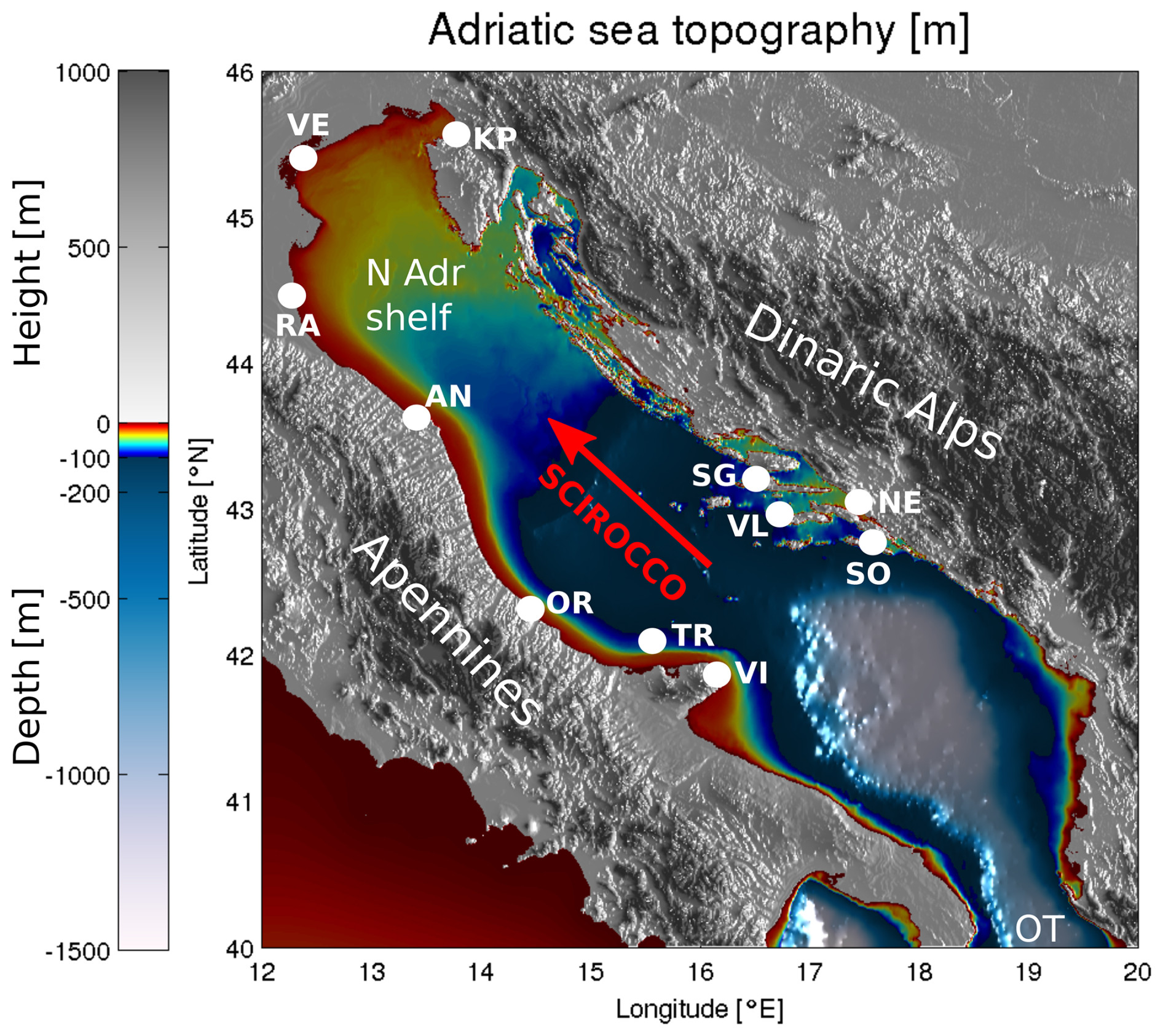
Figure 1 Topography and bathymetry of the Adriatic region. The white dots denote the tide gauges used in this study. The abbreviations used on the map are as follows: KP – Koper, VE – Venice, RA – Ravenna, AN – Ancona, N Adr shelf – northern Adriatic shelf, OR – Ortona, TR – Tremiti, VI – Vieste, SO – Sobra, SG – Stari Grad, VL – Vela Luka, and OT – Otranto. The direction of the scirocco is marked with the red arrow. The image was created by the authors based on General Bathymetric Chart of the Oceans (GEBCO) bathymetry and elevation data available at https://download.gebco.net/ (last access: 14 June 2024).

Numerical general circulation models are commonly used for SSH prediction and provide basin-scale four-dimensional simulations of the full sea state (temperatures, salinities, circulation, and sea levels), whose evolution is nontrivial and numerically demanding (Umgiesser et al., 2022; Ferrarin et al., 2020; Madec, 2016). Furthermore, sea level information in these models typically corresponds to a minor part of the total numerical cost of these simulations, which often involve baroclinic and other processes that have very limited relevance for coastal flood predictions. A further complication arises with the fact that semi-enclosed basins exhibit meteorologically induced standing oscillations or seiches which are superimposed on the tidal sea level signal. This leaves the total sea level highly nonlinearly dependent on the time lag between the peak tide and peak seiche. A possible remedy to this sensitivity is to employ probabilistic or ensemble modeling (Rus et al., 2023; Bernier and Thompson, 2015; Mel and Lionello, 2014) with the hope of efficiently reproducing the envelope of possible sea levels. This approach, however, comes with a high numerical cost, making it unfeasible to run ensemble predictions multiple times a day at national metocean model training dataset services.

To limit the numerical costs, one effective option is to use two-dimensional barotropic models, which have demonstrated efficacy in sea level and ensemble modeling (Bajo et al., 2023; Ferrarin et al., 2023, 2020). Recently, machine learning has emerged as another promising option for reducing numerical costs while enhancing performance. Early models (Imani et al., 2018) used traditional techniques such as support vector machines (SVMs) (Vapnik, 2013), while Ishida et al. (2020) employed long short-term memory (LSTM) networks (Hochreiter and Schmidhuber, 1997) with atmospheric variables for 1 h predictions. Braakmann-Folgmann et al. (2017) extended the prediction horizon using a combination of LSTM networks and convolutional neural networks (CNNs). Autoregressive neural networks were explored in Hieronymus et al. (2019), increasing the temporal resolution and the prediction horizon. While these methods were orders of magnitude faster than their numerical counterparts, their accuracy was generally inferior.

A decisive improvement in accuracy was possible through the employment of deep convolutional architectures from computer vision, such as models from the HIDRA (HIgh-performance Deep tidal Residual estimation method using Atmospheric data) modeling family (Žust et al., 2021; Rus et al., 2023). The HIDRA1 and HIDRA2 networks avoid the need for basin-scale simulations of the full ocean state and focus the network capacity on only predicting sea levels at a single geographic location. HIDRA2 (Rus et al., 2023) has been shown to substantially outperform several numerical models in the speed and accuracy of sea level predictions in Koper (northern Adriatic) and is currently also implemented in the Baltic Sea basin on the Estonian coast (Barzandeh et al., 2024).

The HIDRA2 model currently provides SSH forecasts with a 6 d temporal horizon. Its inputs consist of atmospheric winds and pressures as well as SSH observations in the past 24 h at the prediction location. This means that a sufficiently long history of measured SSH and atmospheric values is required to train HIDRA2 separately at each geographic location. While the atmospheric values are available from sources such as ECMWF (Leutbecher and Palmer, 2007), the SSH values can only be obtained from in situ tide gauges. This brings two main drawbacks. First, for some locations, a long history of SSH measurements is not available, which limits the training capability of HIDRA2, which has to learn not only the SSH information encoding, but also the relevant atmospheric features, the input data fusion process, and the prediction heads. Second, in the case of sensor failure, immediate past observations are unavailable and predictions cannot be made. Several attempts were however made to remedy this situation (Lee and Park, 2016; Vieira et al., 2020).

To address these limitations, we introduce HIDRA3, a new deep-learning architecture designed to simultaneously learn from and predict SSH across multiple tide gauge locations. This new multi-location formulation is the main contribution of this paper. HIDRA3 can further handle missing values in observation datasets at input locations and implicitly reconstruct them in latent space from other available locations. In addition to SSH values, HIDRA3 predicts SSH forecast uncertainties, which enhances the interpretability of the output.

HIDRA3 thus brings several benefits. The prediction accuracy at each individual location is improved by jointly utilizing information from multiple locations. A single HIDRA3 is trained for all locations, and thus many parameters are shared between the locations. This means that locations with scarce historical training data benefit from locations with abundant data. Additionally, this enables predictions even during sensor failures, as HIDRA3 exploits all available observed information at other locations to obtain predictions at locations with missing SSH values. Finally, due to its numerical efficiency, HIDRA3 enables fast and reliable ensemble sea level forecasting multiple times a day.

The remainder of the paper is organized as follows. Section 2 details the new HIDRA3 architecture, Sect. 3 compares HIDRA3 with state-of-the-art numerical and machine-learning models, and conclusions are drawn in Sect. 4.

2 HIDRA3 deep-learning sea level model

2.1 HIDRA3 training and testing datasets

Our objective is to forecast hourly SSH values for N=11 tide gauges located along the Adriatic coast (Fig. 1) over a 3 d period. HIDRA3 achieves this by leveraging a comprehensive set of ocean state parameters. This includes the past 72 h of available sea level observations from the stations shown in Fig. 1, with the data availability for each station detailed in Table 1. When calculating the availability, only SSH measurements with 72 preceding measurements available are considered, as required for HIDRA3 input. Besides past SSH measurements, HIDRA3 considers both past and future astronomic tides at the stations as well as the past and future 72 h of gridded geophysical variables from atmospheric and ocean numerical models.

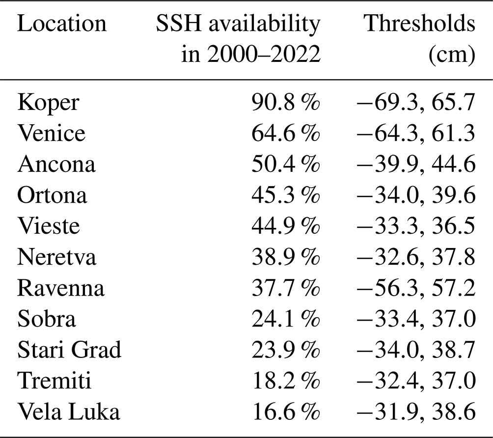
Table 1 Availability of SSH measurements between 2000 and 2022 for the 11 tide gauge locations used in training and evaluating HIDRA3, together with the defined thresholds (1st and 99th percentiles) for the low and high SSH values used in this study. When calculating the SSH availability, only SSH measurements with 72 preceding measurements available are considered, as required for HIDRA3 input. See Fig. 1 for the station locations.

The training time window spans two intervals: from 2000 to 2018 and from 2021 to 2022. The testing time window covers the period from June 2019 to the end of 2020. This specific testing interval was selected due to the occurrence of numerous high-SSH and coastal flood events in the northern Adriatic. During training, we assume that the past 72 h of SSH observations are available for at least one tide gauge in the training set, while they may be missing at several or all other locations. Note that very different amounts of tide gauge data are available at different stations; in particular, all stations situated south of Ancona have a data availability of lower than 50 % throughout the training interval (see Table 1).

In order to eliminate SSH measurement errors, we apply three filters to address three types of errors: (1) sensor freeze, which results in the same value being produced for an extended period of time; (2) extreme outliers; and (3) extreme jumps in the signals. For case (1), we define a threshold of five repetitions, as repetitions typically span more than five time points. For case (2), we define a location-specific threshold equal to 10 times the standard deviation of the measurements and remove all points that are further away from the mean value than that threshold. Note that the threshold needs to be recalculated after each measurement is removed. For case (3), we examine the first derivative of the signals and define a location-specific threshold equal to 10 times the standard deviation of all first derivatives for some location. When two derivatives with opposite signs are close together (fewer than 10 time points), the region between them is removed. Again, it is necessary to recalculate the threshold after each removal. The validity of all the thresholds was verified visually.

Astronomic tides were calculated from tide gauge data in 1-year intervals using the UTIDE Tidal Analysis package for Python (Codiga, 2011). Using 1-year intervals for tidal analysis is a common approach to compensate for the unresolved low-frequency signals in the tidal signal, like the 18.6-year oscillation due to the precession of lunar nodes (Pawlowicz et al., 2002). For each 1-year interval, tidal constituents are inferred from the past year of observations to ensure that no information beyond the prediction point is used. The only exception is in the first year of measurements for each location, when the first year of measurements is used to calculate the first year of tides. This approach is beneficial for training the model and does not affect the evaluation data, as all tide gauges have measurements spanning at least 1 year prior to the test period.

In the context of this analysis, a dataset of sea level extremes was constructed for each station. SSH readings are categorized as low if they are below the 1st percentile and as high if they surpass the 99th percentile of the observed values at the respective location. During evaluation (Sect. 3.2), metrics are calculated for all SSH values as well as low and high values. This helps assess the model's performance in predicting both tails of extreme SSH values: high values are relevant for coastal flood warnings, and low values restrict marine traffic in the shallow north of the basin. The thresholds determined are listed in Table 1.

Tide gauges in the northern Adriatic (Koper, Venice, and Ravenna) and those in the central and southern Adriatic (Ancona, Ortona, Tremiti, Vieste, Sobra, Vela Luka, Neretva, and Stari Grad) form two separate clusters that fall within the barotropic Rossby radii of each other and thus exhibit similar SSH phases of high and low sea levels. This is illustrated in Fig. 2, which depicts the SSH at all the stations, and in Fig. 3, which shows the mean absolute differences between all the stations. These mean absolute differences were calculated using overlapping data from each pair of locations, and they can be interpreted as estimates of the increase in the mean absolute error (MAE) when applying a model's forecast from one location to another.

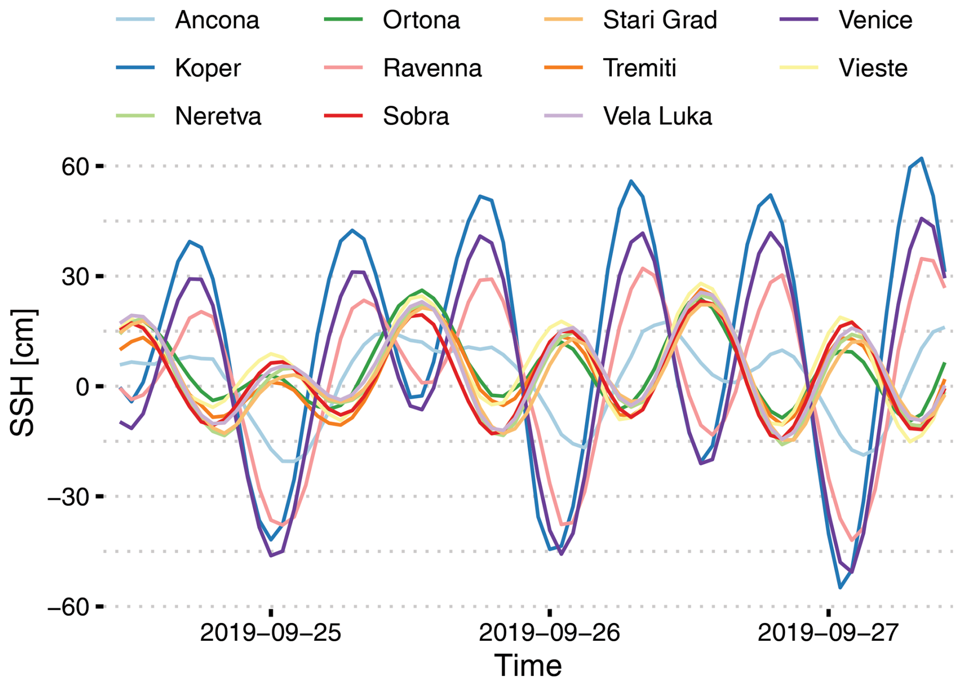
Figure 2 A representative example period of SSH from all 11 tide gauges used in the training and evaluation of HIDRA3.

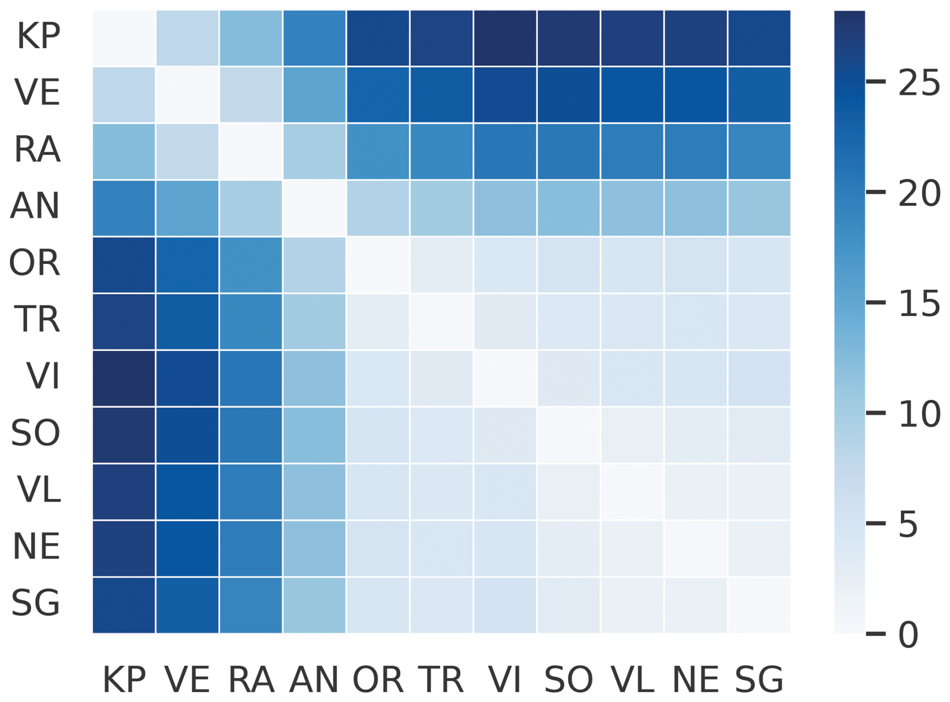
Figure 3 Mean absolute differences (cm) of SSH measurements between different tide gauge locations. These differences estimate the increase in the MAE when applying a model's forecast from one location to another. The abbreviations used here are KP, VE, RA, AN, OR, TR, VI, SO, VL, NE, and SG.

ERA5 reanalysis data (Hersbach et al., 2023) were employed for training purposes, while ECMWF Ensemble Prediction System (EPS) data (Leutbecher and Palmer, 2007) were employed for evaluation to reflect the practical forecasting setup in which future reanalysis does not exist and forecasts are used. To independently verify the impact of the training set, HIDRA3 was also retrained on ECMWF EPS data instead of ERA5. When evaluated on the ECMWF EPS dataset, this led to a slight increase in the MAE (1.7 %). We consequently decided to select the ERA5 dataset for the training.

The metocean model training dataset used in this study consists of 10 m winds, mean sea level air pressure, sea surface temperature (SST), mean wave direction, mean wave period, and significant height of combined wind waves and swell. All the atmospheric model input fields were spatially cropped to the Adriatic basin and subsampled to a 9×12 spatial grid, following our previous work (Rus et al., 2023).

2.2 HIDRA3 model architecture

HIDRA3 proceeds as follows (see Fig. 4 for the architecture). Geophysical variables (wind, air pressure, SST, and waves) are encoded once for all locations in the Geophysical encoder module (Sect. 2.2.1), while the sea level data (full SSH and astronomic tide) and geophysical features are processed separately for each location in the Feature extraction module (Sect. 2.2.2). Features are fused in the Feature fusion module (Sect. 2.2.3), which takes sea level features from locations with available data and encodes them into a single joint state feature vector s, which is decoded by the SSH regression head (Sect. 2.2.4) into the SSH predictions at the individual geographical locations. Finally, the Uncertainty estimation module predicts forecast uncertainties (Sect. 2.2.5).

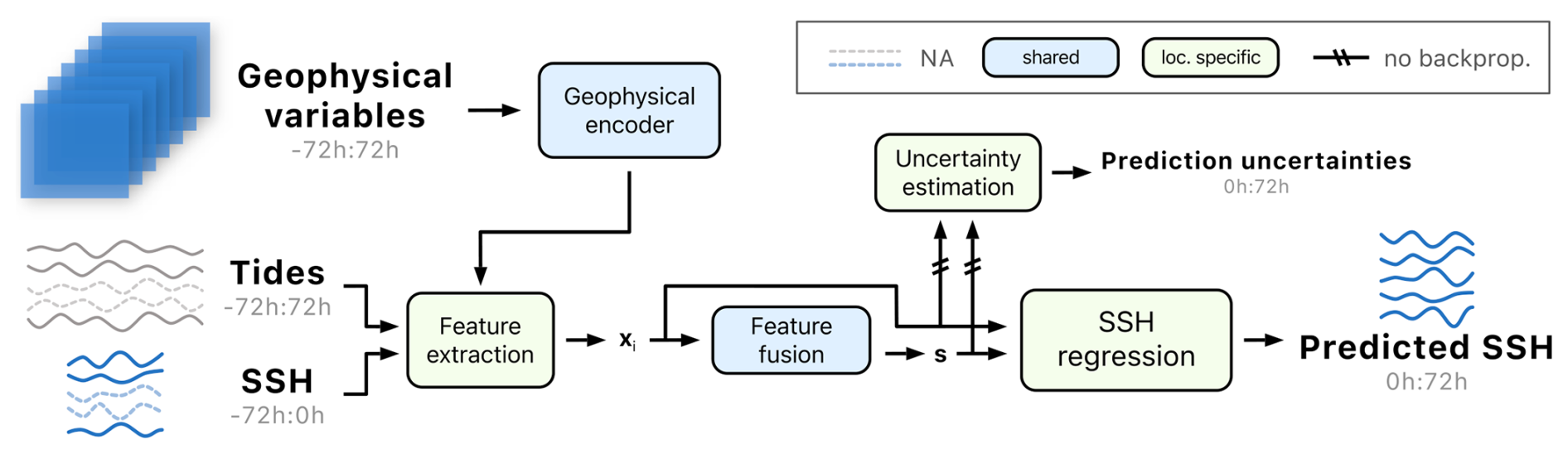
Figure 4 The HIDRA3 architecture. The Geophysical encoder encodes pressure, wind, SST, and waves. The Feature extraction module extracts features separately for each location, creating feature vectors x_i, which are then fused in the Feature fusion module. The SSH regression module produces SSH forecasts, while the Uncertainty estimation module predicts their standard deviations. The location-specific modules and the modules shared by the locations are depicted in green and blue, respectively. Missing SSH data are denoted by a dashed curve. The notation a:b indicates hourly data points from the interval (a,b], while the prediction point is at the index 0.

2.2.1 Geophysical encoder module

The Geophysical encoder takes past and future, i.e., $-\mathrm{72}:\mathrm{72}$ h in hourly steps, geophysical variables as input: wind ($\mathbf{v}=(u_{\mathrm{10}},v_{\mathrm{10}})\in {\mathbb{R}}^{\mathrm{2}\times W\times H}$), pressure ($\mathbf{p}\in {\mathbb{R}}^{W\times H}$), sea surface temperature ($\mathbf{T}\in {\mathbb{R}}^{W\times H}$), and waves ($\mathbf{w}\in {\mathbb{R}}^{\mathrm{4}\times W\times H}$), where W=9 and H=12 are the spatial dimensions of the resampled input fields. The wave tensor w is composed of the following four components (hence the dimension $\mathrm{4}\times W\times H$): the first two are sine and cosine encodings of the mean wave direction, and the remaining two are the mean wave period and significant height of combined wind waves and swell.

The input variables are processed in two steps. In the first step, variables (wind, pressure, SST, and waves) are encoded separately, and then, in the second step, encodings from different variables are fused together. We model each variable independently in the first step to avoid modeling low-level interactions between different variables, which would increase the number of parameters. The first step is shown in Fig. 5. The encoder processes a variable of size $c\times \mathrm{144}\times \mathrm{9}\times \mathrm{12}$ using a three-dimensional convolution block with 64 $\mathrm{2}\times \mathrm{3}\times \mathrm{3}$ kernels with stride $\mathrm{2}\times \mathrm{2}\times \mathrm{2}$ (the first dimension is temporal, while the second two are spatial), followed by a rectified linear unit (RELU), a three-dimensional dropout (Tompson et al., 2014), and another three-dimensional convolution with 512 $\mathrm{2}\times \mathrm{4}\times \mathrm{5}$ kernels with stride $\mathrm{2}\times \mathrm{1}\times \mathrm{1}$. Note that the strides and the kernel sizes are adjusted to reduce the dimensions to $\mathrm{512}\times \mathrm{36}\times \mathrm{1}\times \mathrm{1}$. This adjustment aims to compress the information into a low number of features, which helps reduce the risk of overfitting in the network and limits the number of output features of the Geophysical encoder. For the sea surface temperature and wave variables, the number of kernels in the last convolutional layer is 64 instead of 512, forming an output of size $\mathrm{64}\times \mathrm{36}\times \mathrm{1}\times \mathrm{1}$. This modification has led to a marginal enhancement in the performance, presumably due to the larger number of features representing wind and pressure compared to SST and waves, thereby assigning greater significance to the former variables, which have more relevance in the context of SSH forecasting.

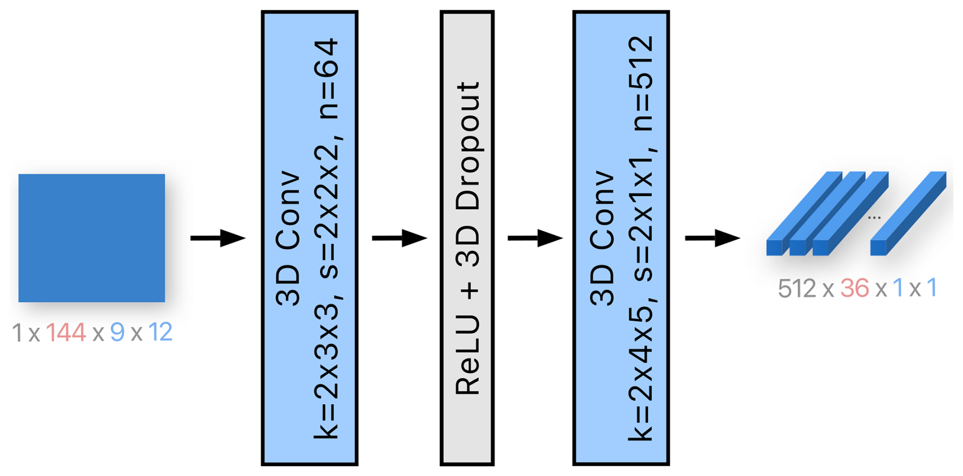
Figure 5 The first step of the Geophysical encoder module involves encoding each of the four variables separately. Note that wind has two input channels, while the wave data have four. The encoder consists of two three-dimensional convolutions, reducing the spatial dimension to 1×1. Wind and pressure are encoded into 512 output channels, as depicted in the figure, while sea surface temperature and wave data are encoded into 64 channels. The variables k, s, and n denote the kernel size, the stride, and the number of output channels, respectively. The number of channels is indicated in gray, the size of the temporal dimension is in red, and the spatial dimensions are in blue.

Encodings from all the variables are concatenated, resulting in a total of $\mathrm{2}\cdot \mathrm{512}+\mathrm{2}\cdot \mathrm{64}=\mathrm{1152}$ channels. By removing spatial dimensions of size 1, concatenation has size 1152×36, which is then the second step of the Geophysical encoder (see Fig. 6) processed by a one-dimensional convolution with 256 kernels of temporal size 5. We have chosen the kernel size of 5 to increase the receptive field of the layer, which, with this setup, covers approximately 20 h. We have found this to be effective in preliminary studies (not shown here). Next, two one-dimensional convolutions with 256 kernels of temporal size 1 are applied and are followed by a scaled exponential linear unit (SELU) activation (Klambauer et al., 2017), one-dimensional dropout, and a residual connection (see Fig. 6). These layers enable the extraction of more complex features from the geophysical variables. After flattening, the output is a single vector of 8192 geophysical features.

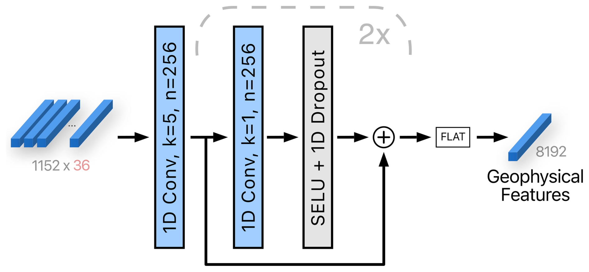
Figure 6 The second step of the Geophysical encoder module. Geophysical variables that were encoded independently in the first step are fused to form a single vector. One-dimensional convolutions with residual connections and nonlinearities are applied to produce 256×32 output, which is then flattened into a single vector of all the geophysical features. The variables k and n denote the kernel size and the number of output channels, respectively. The number of channels is indicated in gray, and the size of the temporal dimension is in red. The block marked with a dashed line is repeated twice.

2.2.2 Feature extraction module

At the prediction time, some tide gauges may not have measurements available, e.g., due to temporary sensor failures. Therefore, in the Feature extraction module, the location-specific features x_i are extracted independently for each location. Then, in the Feature fusion module, the features from all the stations are merged, taking into account the fact that the data at some of the locations are unavailable.

As visualized in Fig. 7, the SSH observations (72 values) and the astronomic tide (144 values) are concatenated and encoded with a dense layer (i.e., a fully connected layer) with 512 output channels. Geophysical features are also passed through a dense layer with 512 output channels whose task is to extract the features relevant to the specific tide gauge. The outputs of both layers are concatenated and processed with four dense layers with 1024 output channels. A SELU, a dropout, and residual connections are applied as shown in Fig. 7. The skip-connection-based approach is chosen for its excellent feature construction ability, which proceeds by adding nonlinearly transformed input features as residuals to the original features. This, in practice, leads to better training behavior due to a steeper gradient in the backpropagation phase (He et al., 2016). We chose SELU (Klambauer et al., 2017) for its smoother gradient propagation properties compared to its RELU counterpart, while the dropout is employed as a classical technique to curb overfitting.

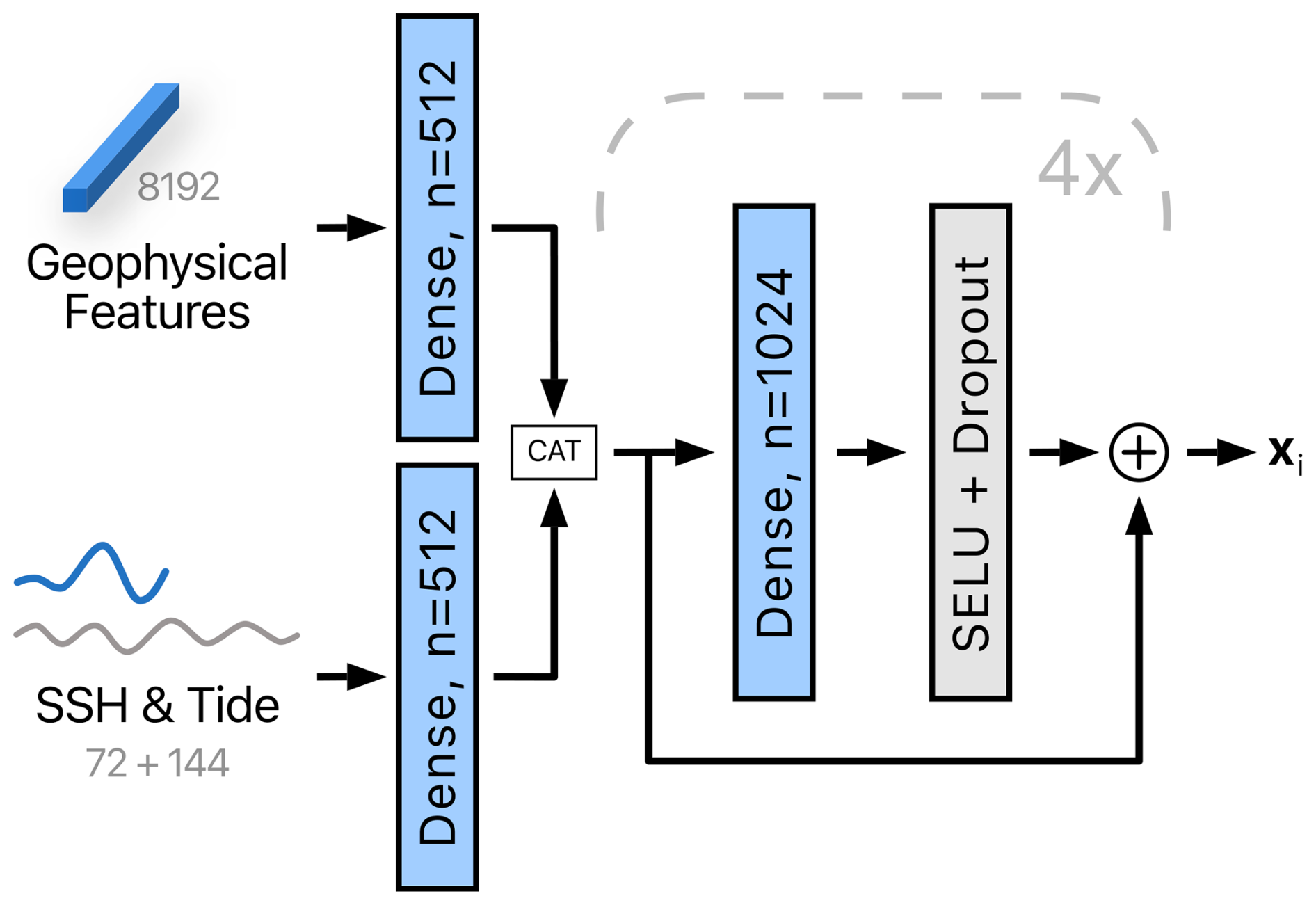
Figure 7 The Feature extraction module has geophysical features, observed SSH measurements, and astronomic tide forecasts, which are processed independently for each location to extract location-specific features x_i. The variable n denotes the number of output channels. The data dimensions are indicated in gray. The block marked with a dashed line is repeated four times.

2.2.3 Feature fusion module

As indicated in Fig. 4, the Feature fusion module combines the location-specific features x_i∈ℝ¹⁰²⁴ into a joint state vector s∈ℝ⁸¹⁹². A critical design requirement for the module is robustness to missing data; specifically, the number of location-specific features x_i may vary, as they are only available for tide gauges with available measurements.

A partial reconstruction s_i of the state is computed from each location-specific feature vector x_i by applying a location-specific dense layer (see Fig. 8). In addition, a weight vector w_i is computed by applying another location-specific dense layer to x_i. Each coordinate in w_i reflects the extent to which the particular location contributes to the respective coordinate in the joint state vector. If some tide gauges are nondescriptive, their weights will be reduced during training, lowering their influence on the final state vector s, which is thus computed as

$$\begin{array}{}\text{(1)}& \mathit{s}=\sum _{i\in V}{\widehat{\mathit{w}}}_i\odot {\mathit{s}}_i,\end{array}$$

where ⊙ denotes element-wise array multiplication, ${\widehat{\mathit{w}}}_i$ are the coordinate-normalized weight vectors, and V contains indices of tide gauges with available SSH measurements, so that s is approximated from tide gauges with available measurements. The components ${\widehat{w}}_{i,j}$ are computed by a softmax, i.e.,

$$\begin{array}{}\text{(2)}& {\widehat{w}}_{i,j}={\displaystyle \frac{e^{w_{i,j}}}{{\sum }_{k\in V}{e}^{w_{k,j}}}},\end{array}$$

where the softmax ensures that the coordinate-wise weights sum to 1 across all locations with available measurements.

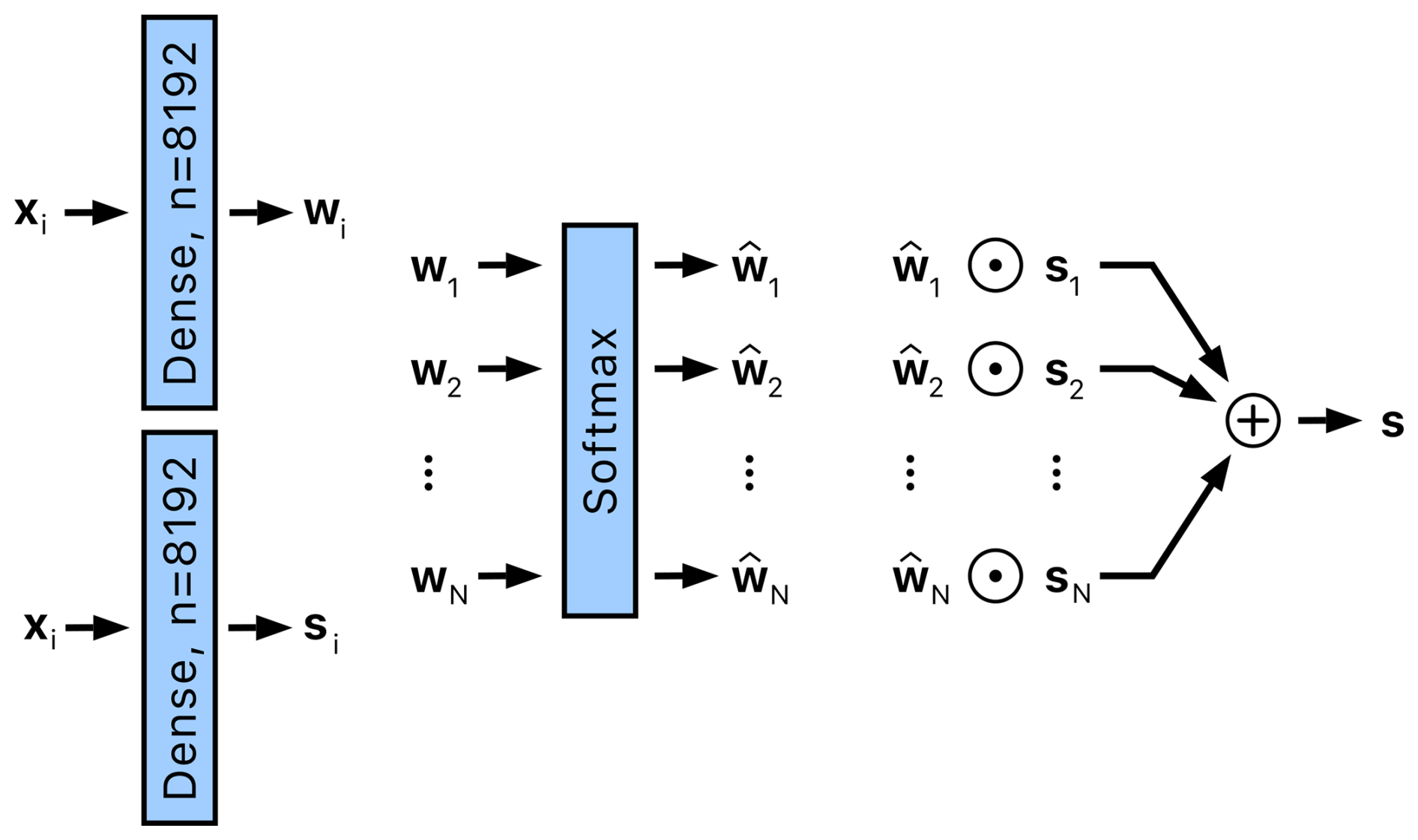
Figure 8 The Feature fusion module takes features x_i from location i and uses them to generate weights w_i and a partial reconstruction of state s_i. These weights and partial reconstructions are combined into a joint state vector s using weighting and aggregation mechanisms. Locations without available measurements are excluded from the softmax calculation and aggregation. The parameters of the dense layers are specific to each location. The element-wise multiplication is denoted by the symbol ⊙.

2.2.4 SSH regression module

The ith SSH regression module receives the joint state vector s. However, since some stations may be de-prioritized in the state vector by the Feature fusion module, i.e., due to a smaller amount of training data available for that station, the state vector is concatenated with a station-specific feature vector ${\widehat{\mathit{x}}}_i$. The concatenated feature vector is then processed using a dense layer with 72 output features to regress the 72 hourly SSH predictions ${\widehat{\mathit{\mu }}}_i$.

Note that two situations emerge in the construction of the station-specific feature vector ${\widehat{\mathit{x}}}_i$, depending on the sensor data availability. If the measurements are available for the ith tide gauge, the station-specific feature vector is simply obtained by passing the features computed for the respective tide gauge x_i (Sect. 2.2.2) through a dense layer with 1024 output features. This nonlinear transformation is applied to enable the network to emphasize the part of the feature vector that is possibly underrepresented in the joint state vector. However, if the measurements are unavailable, e.g., due to sensor failure, then a station-specific feature vector is approximated by transforming the joint state vector, i.e., passing it through a dense layer with 1024 output features (see Fig. 9).

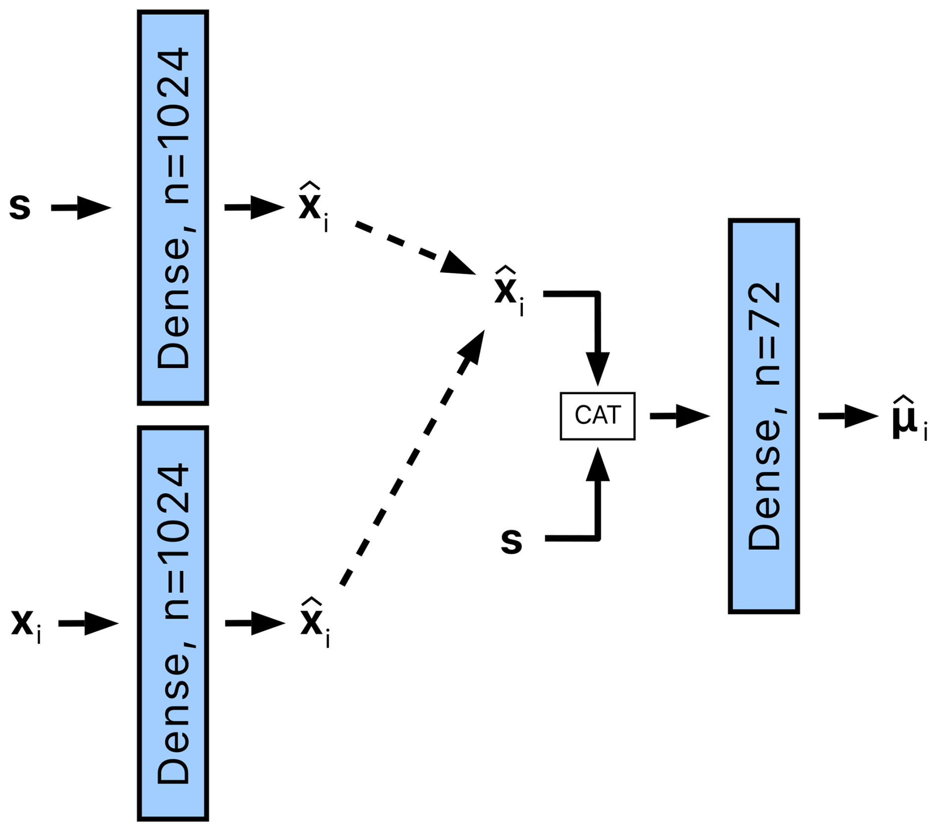
Figure 9 The SSH regression module for a location i receives a joint state vector s and location-specific features x_i. The features x_i are processed by a dense layer to produce the features ${\widehat{\mathit{x}}}_i$. In cases where measurements from the tide gauge at location i are unavailable and therefore x_i is undefined, ${\widehat{\mathit{x}}}_i$ is approximated from s using a separate dense layer. The features ${\widehat{\mathit{x}}}_i$ and s are then concatenated and passed through a final dense layer to obtain SSH predictions denoted as ${\widehat{\mathit{\mu }}}_i$.

2.2.5 Uncertainty estimation module

Finally, the Uncertainty estimation module predicts the hourly standard deviations corresponding to the SSH estimate ${\widehat{\mathit{\mu }}}_i$. This module has the same architecture as the last layer of the SSH regression module (Sect. 2.2.4), with one slight distinction: it applies a soft-plus function (Glorot et al., 2011) to the output to ensure the positivity of the estimated standard deviation vector ${\widehat{\mathit{\sigma }}}_i$.

2.3 Training and implementation details

Training is split into two phases. In the first phase, SSH prediction is trained using the mean squared error (MSE) loss between the SSH predictions and the ground truth. We use an AdamW (Loshchilov and Hutter, 2017) optimizer with a learning rate of $\mathrm{1}\times {\mathrm{10}}^{-\mathrm{5}}$ and a weight decay of 0.001. We apply the cosine annealing (Loshchilov and Hutter, 2016) learning schedule to gradually reduce the learning rate by a factor of 100. To simulate tide gauge failures during training, a random number of tide gauges are turned off with a probability of 0.5. The batch size is set to 128 data samples, and the model is trained for 20 epochs. All the input data are standardized by subtracting the mean and dividing by the standard deviation. For each tide gauge location, the mean is calculated independently, while a single standard deviation is computed across all the locations. Each geophysical variable is standardized independently of the other variables. Training takes approximately 1 h on a computer with an NVIDIA A100 Tensor Core GPU graphics card.

In the second phase, uncertainty prediction is trained. The second phase needs to have a different training dataset, which is necessary for preventing the underestimation of the uncertainty. Hence, only the year 2020 was used to train the second phase. In the second phase, the negative log-likelihood is optimized:

$$\begin{array}{}\text{(3)}& \mathcal{L}=-{\displaystyle \frac{\mathrm{1}}{N}}\sum _{i=\mathrm{1}}^N\sum _{t=\mathrm{1}}^{\mathrm{72}}\log {\displaystyle \frac{\mathrm{1}}{{\widehat{\mathit{\sigma }}}_{i,t}}}\exp \left[-{\displaystyle \frac{({\mathit{\mu }}_{i,t}-{\widehat{\mathit{\mu }}}_{i,t}{)}^{\mathrm{2}}}{{\widehat{\mathit{\sigma }}}_{i,t}^{\mathrm{2}}}}\right],\end{array}$$

where μ_i,t is the ground truth SSH value for the ith tide gauge at prediction lead time t, ${\widehat{\mathit{\mu }}}_{i,t}$ is the predicted SSH value, and ${\widehat{\mathit{\sigma }}}_{i,t}$ is the predicted standard deviation. The second phase applies a learning rate of $\mathrm{1}\times {\mathrm{10}}^{-\mathrm{4}}$ for 40 epochs; batch size, weight decay, and learning rate schedule are the same as in the first phase.

In operational forecasting, and for the evaluation, an ensemble of n_ens=50 atmospheric members is utilized. HIDRA3 processes each member individually, yielding 50 SSH forecasts and the associated standard deviations at each time step. These are merged into a single probabilistic forecast through Gaussian moment matching (Kristan and Leonardis, 2013). The prediction is the average of all ensemble forecasts, while the variance is computed as follows:

$$\begin{array}{}\text{(4)}& {\stackrel{\mathrm{‾}}{\mathit{\sigma }}}_t^{\mathrm{2}}={\displaystyle \frac{\mathrm{1}}{n_{\mathrm{ens}}}}\sum _{i=\mathrm{1}}^{n_{\mathrm{ens}}}({\widehat{\mathit{\sigma }}}_{t,i}^{\mathrm{2}}+{\widehat{\mathit{\mu }}}_{t,i}^{\mathrm{2}})-{\left({\displaystyle \frac{\mathrm{1}}{n_{\mathrm{ens}}}}\sum _{i=\mathrm{1}}^{n_{\mathrm{ens}}}{\widehat{\mathit{\mu }}}_{t,i}\right)}^{\mathrm{2}},\end{array}$$

where ${\widehat{\mathit{\mu }}}_{t,i}$ denotes the SSH forecast at time t for ensemble member i and ${\widehat{\mathit{\sigma }}}_{t,i}$ represents the corresponding standard deviation estimate.

2.3.1 Network initialization

Considering the complex information flow from many variables that exist on different scales and are represented by latent descriptors of different sizes in the network, care is required at training-time parameter initialization. The weights of convolutional and dense layers are initialized using a standard Xavier initialization (Glorot and Bengio, 2010), while biases are initialized using a normal distribution with a standard deviation of 0.1. In the Feature extraction module, the deeper layers are given lower initial weights, assigning less significance to complex features during the initialization phase. Specifically, for each of the four recurrent dense layers in the Feature extraction module, the weight and bias are scaled by a factor of 0.5ⁱ⁻¹, where i represents the layer's position in the sequence, ranging from 1 to 4.

In the SSH regression module and the Uncertainty estimation module, an additional step of weight scaling is implemented during initialization. In the module, s and ${\widehat{\mathit{x}}}_i$, which have different dimensions, are concatenated. To ensure that the contributions of s and ${\widehat{\mathit{x}}}_i$ to the final output are initially proportionally balanced, the ratio of their sizes is used to scale the weights of the final dense layer in the SSH regression module and the Uncertainty estimation module.

2.4 Summary of the differences from HIDRA2

HIDRA3 presents a significant advancement over its predecessor HIDRA2 (Rus et al., 2023) by introducing the ability to simultaneously process data from multiple tide gauge locations. This required a major redesign of the model, as HIDRA3 must effectively handle scenarios where SSH measurements are not available.

The only similar part is the Geophysical encoder module, albeit with a difference in the way temporal data are processed. In HIDRA2, there is a 4 h temporal reduction in the atmospheric data, while HIDRA3 incorporates the temporal reduction directly into the convolutional operations of the Geophysical encoder module. Additionally, HIDRA3 expands its input data to include sea surface temperature and wave fields and considers not only the past 24 h like HIDRA2, but also the 72 h before the prediction point.

A notable contribution of HIDRA3 is its capacity for uncertainty quantification, a feature that was absent in HIDRA2. This ability is crucial for assessing the reliability and potential limitations of the SSH forecasts generated by the model.

3 Results

3.1 Nucleus for European Modelling of the Ocean (NEMO) model description

We compare HIDRA3 with the state-of-the-art deep-learning model HIDRA2 (Rus et al., 2023) and with the standard Copernicus Marine Environment Monitoring Service (CMEMS) product MEDSEA_ANALYSISFORECAST_PHY_006_013 (Clementi et al., 2021) based on the numerical model NEMO v4.2 (Madec, 2016). The Mediterranean Sea Physical Analysis and Forecasting model (MEDSEA_ANALYSISFORECAST_PHY_006_013) operates on a regular grid with a horizontal resolution of $\mathrm{1}/\mathrm{24}$° (approximately 4 km) and 141 vertical levels. It uses a staggered Arakawa C grid with masking for land areas and a z^* vertical coordinate system with partial cells to accurately represent the model topography. The model incorporates tidal forcing using eight components (M2, S2, N2, K2, K1, O1, P1, and Q1) and is forced at its boundaries by the Global analysis and forecast product (GLOBAL_ANALYSISFORECAST_PHY_001_024) on the Atlantic side. While in the Dardanelles, it uses a combination of daily climatological fields from a Marmara Sea model and the global analysis product. Atmospheric forcing comes from the ECMWF forecasting product. Initial conditions are taken from the World Ocean Atlas (WOA) 2013 V2 winter climatology as of 1 January 2015. Data assimilation is performed using the OceanVar (3DVAR) scheme, which integrates in situ vertical profiles of temperature and salinity from ARGO, Glider, and XBT as well as sea level anomaly (SLA) data from multiple satellites (including Jason 2 and 3, SARAL (ALtiKa), CryoSat, Sentinel-3A and Sentinel-3B, Sentinel-6A, and HY-2A and HY-B). The hydrodynamic part of the model is coupled to the wave model WaveWatch-III. Further information about the model is available in Clementi et al. (2021).

Since NEMO predicts the full ocean state, including SSH, on a regular grid, the respective tide gauge locations are approximated by the nearest-neighbor locations in the grid. One important thing to note is that ocean models like NEMO calculate sea surface height as a local departure from the geoid in the computational cell. A typical cell dimension is on the order of hundreds of meters. This means that the model's SSH represents a departure from the geoid averaged over hundreds of square meters and is not directly related to the in situ observations from local tide gauges, which measure local water depth. Therefore, to align NEMO forecasts with the local tide gauge water depth, an offset adjustment of the initial 12 h forecast is necessary to ensure zero bias compared to the respective tide gauge, as explained in Rus et al. (2023).

3.2 SSH forecast performance

The following performance measures (Rus et al., 2023) are employed: MAE, RMSE, accuracy (ACC), bias, recall (Re), precision (Pr), and F₁ score. Additionally, we calculate the normalized mean absolute error (nMAE) by dividing the MAE score for each location by the standard deviation of all historical SSH measurements for that location. These performance metrics are reported in Table 2 separately for all SSH values (overall) and for low and high SSH values (see Sect. 2 for the definitions).

Table 2 Performance calculated on all SSH values, low SSH values, and high SSH values, averaged over all the locations. The proposed HIDRA3 has the best performance overall and on high SSH values as well as a performance comparable to HIDRA2 on low SSH values. Bold values indicate the best performance in each part of the table.

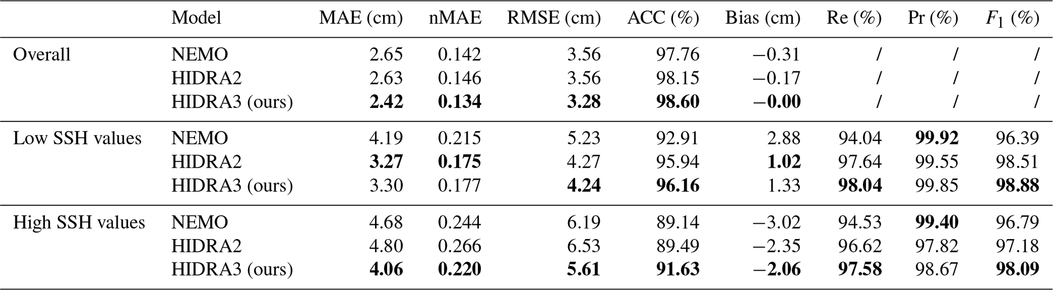
Table 2 shows that HIDRA3 outperforms both competing models across all metrics computed for all SSH values and for high SSH values. Notably, HIDRA3 achieves an 8.0 % lower MAE compared with HIDRA2 (Rus et al., 2023) and an 8.7 % lower MAE compared with NEMO (Madec, 2016). On high SSH values, HIDRA3 achieves a 15.4 % lower MAE than HIDRA2 and a 13.2 % lower MAE than NEMO. These trends are consistent across other evaluation metrics. Furthermore, HIDRA3 demonstrates a near-zero bias and achieves the highest recall on both low and high SSH values among the models. While NEMO has a slightly higher precision, this comes at the cost of a lower recall, implying missed events, while HIDRA3 exhibits a solid balance between precision and recall, as evidenced by its highest F₁ score for both low and high SSH values.

Figure 10 shows the MAE separately for each tide gauge location. Prediction is most challenging for the northern locations, which yield comparatively larger errors than the other locations. This is likely due to shallow waters and topographic amplifications in the northern Adriatic. Under these conditions, however, HIDRA3 demonstrates the most significant improvement in MAE when compared with NEMO. In Koper, the MAE is lower by 22.6 % and 27.7 % on high SSH values, in Venice by 19.0 % and 22.2 % on high SSH values, and in Ravenna by 13.9 % and 30.0 % on high SSH values. On the other hand, the southern locations show much smaller and comparable MAE errors with both NEMO and HIDRA3, which is also due to the overall lower sea level variability in the deeper southern part of the basin with less topographic amplification.

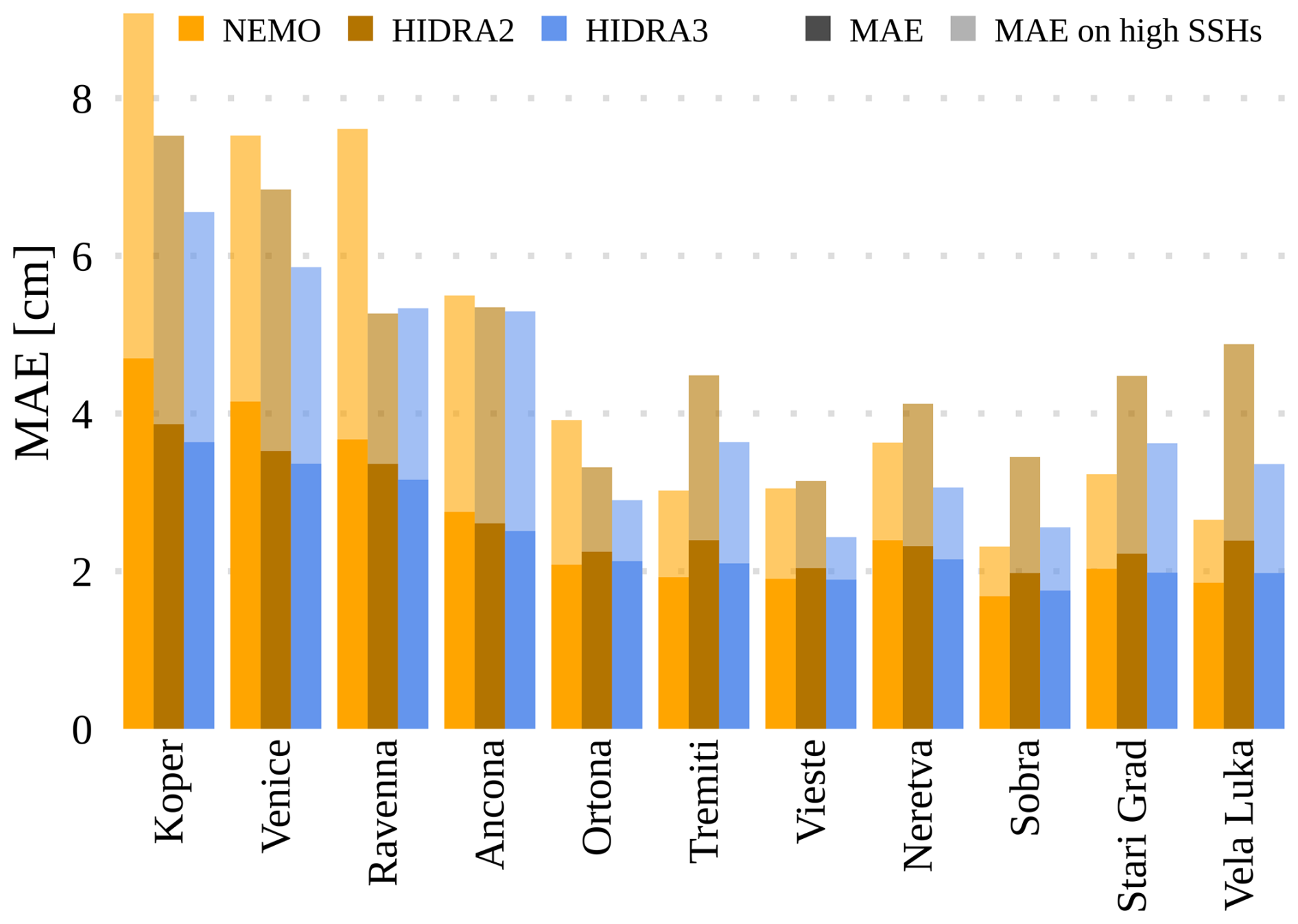
Figure 10 The overall MAE and the MAE on high SSH values calculated for different models and tide gauge locations. HIDRA3 significantly outperforms HIDRA2 (Rus et al., 2023) and also outperforms NEMO (Madec, 2016) at the northern locations.

To enable a more effective comparison of errors across different locations, we present the nMAE in Fig. 11. Although the scores are normalized, NEMO still shows the largest errors at the northern locations (Koper, Venice, and Ravenna). In contrast, HIDRA2 records larger normalized errors at the southern locations, likely due to the lower data availability in those areas (see Table 1). HIDRA3 demonstrates the most consistent performance, significantly outperforming NEMO at the northern locations and HIDRA2 at the southern locations. On average, HIDRA3 has a lower nMAE score than both NEMO and HIDRA2 when calculated on all SSH values and high SSH values (see Table 2).

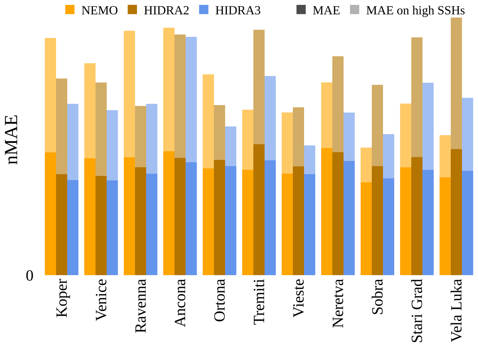
Figure 11 The normalized MAE (nMAE) calculated for all SSH values and high SSH values across the different models and tide gauge locations. HIDRA3 demonstrated the most consistent performance, significantly outperforming NEMO (Madec, 2016) at the northern locations (Koper, Venice, and Ravenna) and HIDRA2 (Rus et al., 2023) at the other locations.

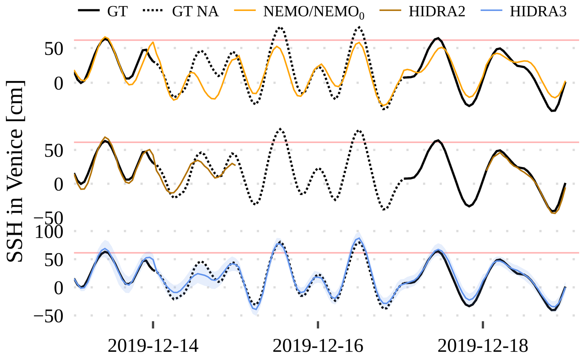
Figures 12 and 13 visualize December 2019 flooding predictions for Venice and Stari Grad, respectively. The first 24 h of daily predictions were concatenated for each model to get a single time series. In Venice (Fig. 12), HIDRA3 predictions most accurately match the ground truth observations. For instance, NEMO fails to predict the 14–16 December floods, while HIDRA3 captures them very well. Also, during the peaks in the second part of the month, HIDRA3 is the most accurate.

In Stari Grad (Fig. 13), the first peak is missed by all the models, while subsequent peaks above the high SSH threshold and low water levels are predicted most accurately by HIDRA3. NEMO and HIDRA2 often underestimate the range of sea level variability in Stari Grad, with maxima being too low and minima being too high. HIDRA3, on the other hand, produces a solid forecasting result, even though the training data availability in Stari Grad is merely 23.9 % (see Table 1).

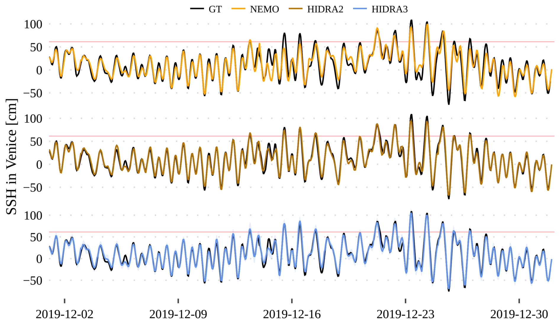
Figure 12 Comparison of the HIDRA3, HIDRA2, and NEMO predictions with the ground truth (black line) in the December 2019 floods in Venice. The high SSH threshold is marked with a red line.

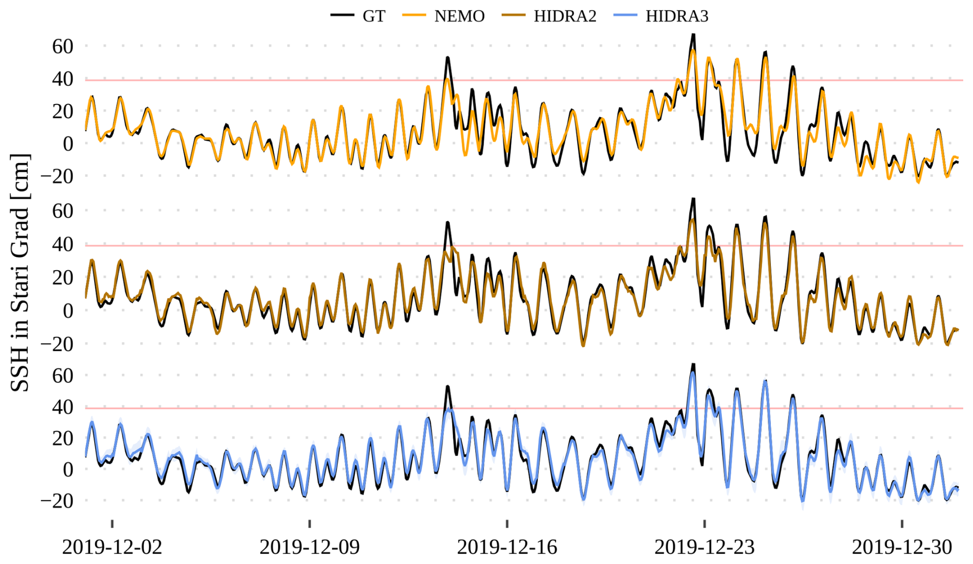
Figure 13 Comparison of the HIDRA3, HIDRA2, and NEMO predictions with the ground truth (black line) in the December 2019 floods in Stari Grad (Hvar, Croatia). The high SSH threshold is marked with a red line.

3.3 Uncertainty estimation analysis

Besides the forecasted SSH values, HIDRA3 also estimates uncertainties by predicting the standard deviation for each forecasted value. To assess the reliability of the estimated standard deviations, we employ the scaled error metric

$$\begin{array}{}\text{(5)}& {\mathit{ϵ}}_{i,t}={\displaystyle \frac{{\mathit{\mu }}_{i,t}-{\widehat{\mathit{\mu }}}_{i,t}}{{\widehat{\mathit{\sigma }}}_{i,t}}}\end{array}$$

as proposed by Barth et al. (2020). This metric quantifies the difference between the ground truth SSH value μ_i,t and the predicted SSH value ${\widehat{\mathit{\mu }}}_{i,t}$, scaled by the estimated standard deviation ${\widehat{\mathit{\sigma }}}_{i,t}$, where i is the tide gauge index and t is the prediction lead time. To assess the accuracy of our predicted uncertainty, we calculate the mean μ_ϵ and standard deviation σ_ϵ of the scaled error. If the predicted and observed error distributions align, the standard deviation of the scaled error should be σ_ϵ=1.0.

For the second half of the 2019 data, which was not used in the training, the standard deviation of the scaled error for HIDRA3 is σ_ϵ=0.98. This indicates that HIDRA3 has good uncertainty prediction abilities, with a slight overestimation of the standard deviations of the prediction errors. To further analyze the distribution of the scaled error metric ϵ_i,t, we plot its histogram in Fig. 14, along with the ideal model (a zero-centered unit-sigma Gaussian) and the Gaussian distribution characterized by the estimated mean μ_ϵ and standard deviation σ_ϵ of HIDRA3. Note that the estimated Gaussian distribution aligns well with the distribution of the ideal uncertainty prediction model, suggesting that HIDRA3 has excellent uncertainty prediction abilities.

Figure 14 Histogram of the scaled error ϵ_i,t, overlaid with an ideal Gaussian distribution with mean 0 and variance 1 and a Gaussian distribution characterized by the estimated mean μ_ϵ and standard deviation σ_ϵ from HIDRA3. The estimated Gaussian distribution aligns well with the ideal one, suggesting excellent uncertainty prediction abilities of HIDRA3.

3.4 Evaluation under tide gauge failures

3.4.1 Single tide gauge failure

To evaluate the robustness of HIDRA3 to tide gauge failures, we simulated the failures at each location by taking the SSH measurements at a location that was unavailable at the prediction time. In such a scenario, HIDRA2 (Rus et al., 2023) is unable to produce predictions. For NEMO, a tide gauge failure primarily means that the bias offset adjustment, which translates the predicted SSH (over the geoid) into the total water level, is not available. Consequently, we offset the NEMO SSH at the location of the failed tide gauge using the average bias of all the non-failed locations. We refer to this offset version of NEMO results as NEMO₀.

The average performance over all locations with the failed tide gauges is shown in Table 3 and visualized in Fig. 15. HIDRA3 achieves a lower MAE than NEMO₀ across all the locations, most notably in Koper. We emphasize that this is not equal to the error of the NEMO model but is rather a demonstration of an expected error in case of a sensor failure, where we are forced to infer offset adjustment from available stations.

Note that, for the majority of the southern locations, the MAE on high SSH values is higher for HIDRA3 than NEMO₀, with the differences being quite small. Nevertheless, in Koper, HIDRA3 outperforms NEMO₀ by a large margin and attains a lower mean MAE on high SSH values. This is also reflected in the other metrics reported in Table 3.

Table 3 Performance of HIDRA3 and NEMO₀ under the target location tide gauge failure. Bold values indicate the best performance in each part of the table.

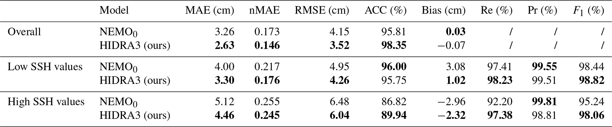
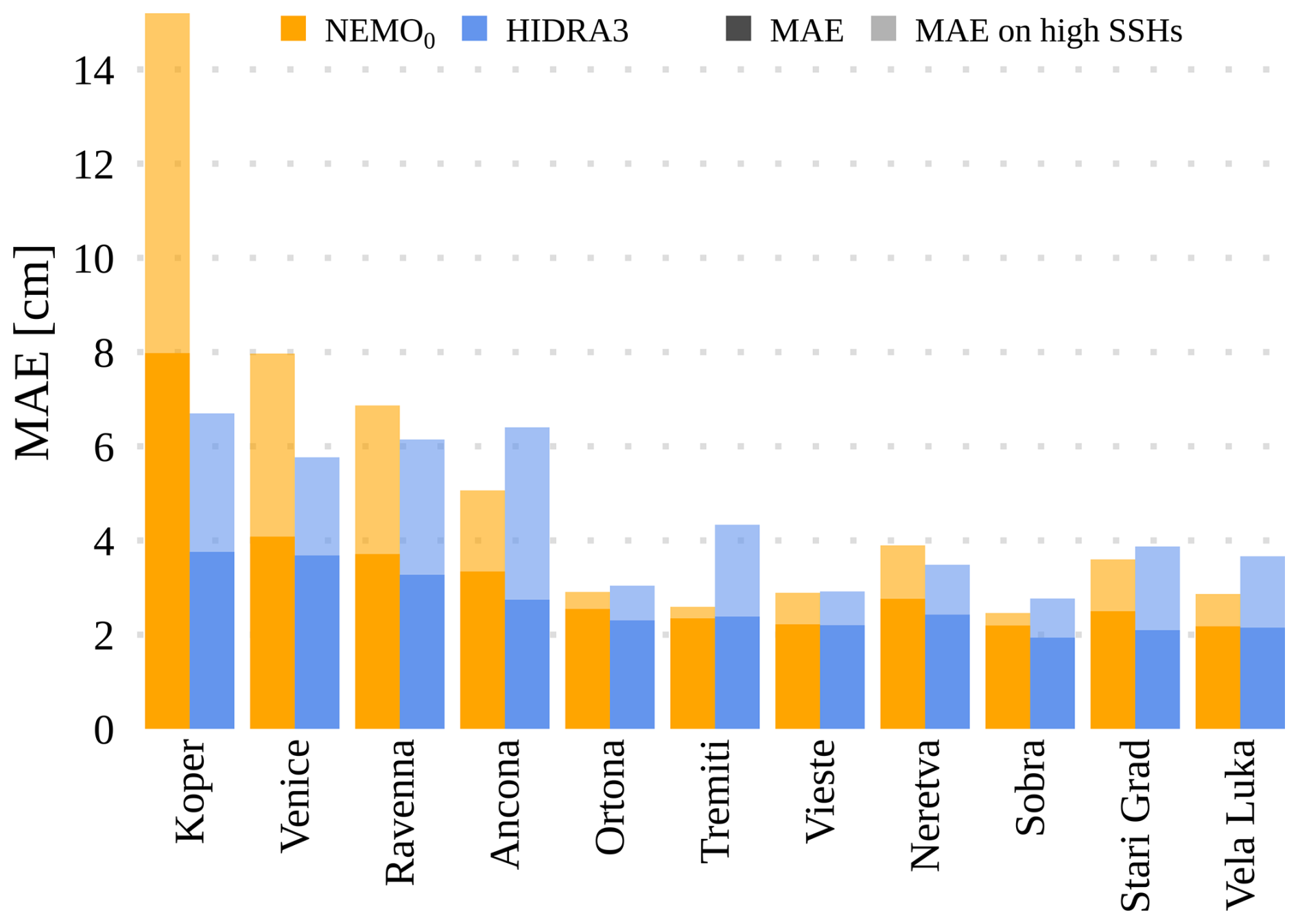
Figure 15 The overall MAE and the MAE on high SSH values calculated for locations with simulated single (isolated) sensor failures at stated locations (x axis). Note that the increased NEMO₀ errors compared to the NEMO errors in Fig. 10 are due to a lower bias correction quality during periods of local sensor failures.

We next simulated a pair of tide gauge failures: the one close to the mouth of the Neretva River, Croatia, and the Venice tide gauge. Figures 16 and 17 show the corresponding SSH observation time series along with the concatenation of the first 24 h of six daily forecasts. While the previous HIDRA2 cannot predict during tide gauge failures, HIDRA3 seamlessly predicts SSH values, with errors lower than NEMO₀.

Figure 16 Forecasts of the December 2019 floods at the Neretva tide gauge with simulated single (isolated) sensor failure. The SSH measurements are shown in black, while the dotted lines indicate the failure simulations. HIDRA2 is unable to make predictions during sensor failure, while HIDRA3 continues to deliver reliable predictions. A band of 2 standard deviations is drawn around the HIDRA3 predictions to visualize the estimated uncertainty. The red lines indicate high SSH values.

Figure 17 Same as Fig. 16 but for the Venice tide gauge.

3.4.2 Extreme scenario of a regional tide gauge failure

To evaluate the model's performance in an extreme scenario of a regional tide gauge failure, we conducted an additional experiment where all the northern locations (Koper, Venice, and Ravenna) were disabled. These locations exhibit distinct dynamical characteristics compared to the others, as illustrated in Figs. 2 and 3. The evaluation of HIDRA3 without SSH measurements from Koper, Venice, and Ravenna is denoted as HIDRA3_S. Importantly, the model was not retrained for this experiment; rather, the same model trained on all the locations was used, with the specified measurements withheld from the test set. This stress test quantifies HIDRA3 predictions for northern tide gauges based exclusively on data from southern tide gauges.

Figure 18 compares the MAE scores of HIDRA3_S, HIDRA3, and NEMO. Surprisingly, HIDRA3_S demonstrates robust forecasting abilities at the northern locations, despite lacking direct measurements. While the MAE scores are slightly higher than those obtained with all the locations as inputs (HIDRA3), they significantly outperform NEMO. At the southern locations, the performance of HIDRA3 and HIDRA3_S is comparable and worse than NEMO. This is expected given the availability of past SSH measurements for these regions.

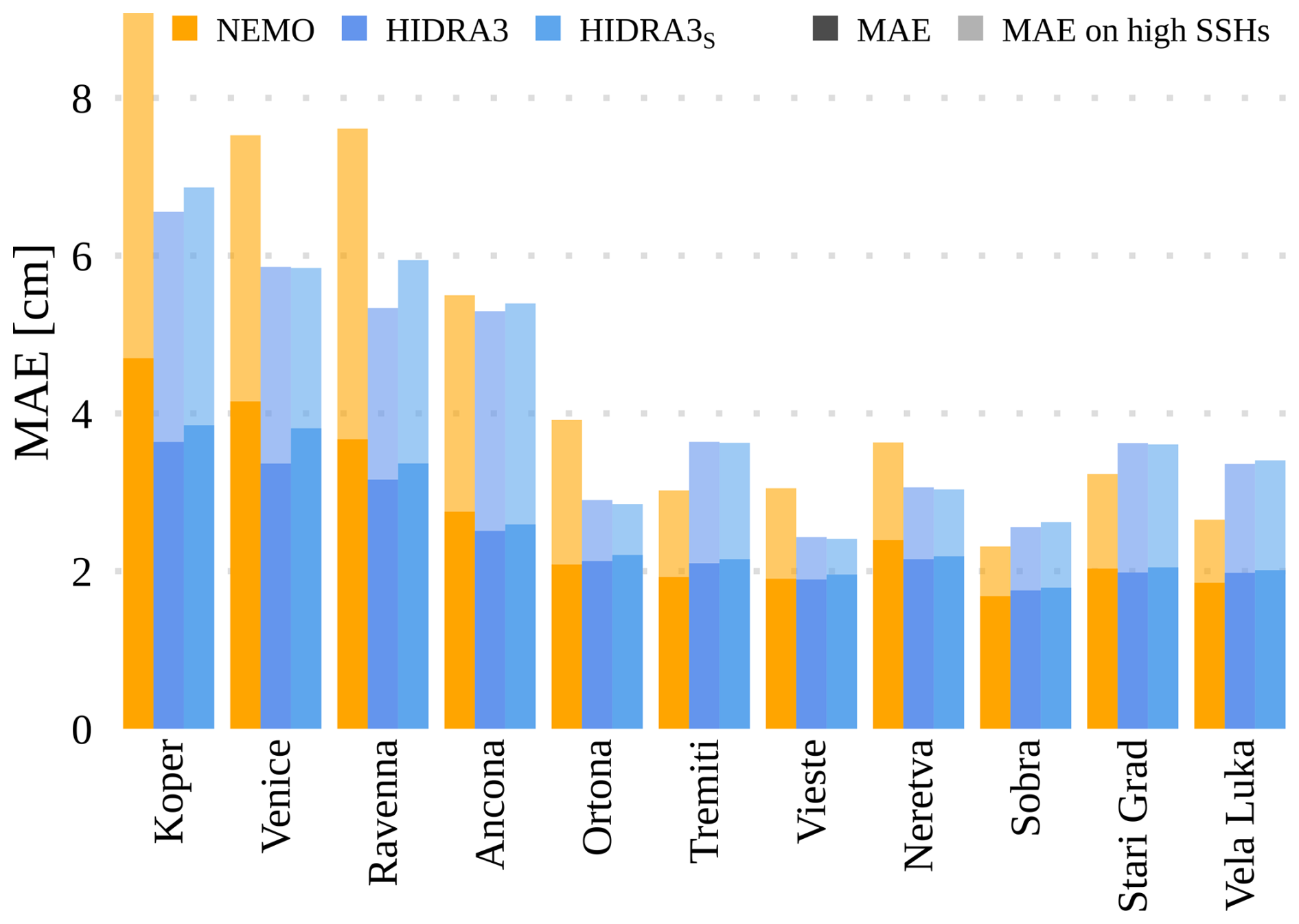
Figure 18 Multiple sensor failure scenario: overall (dark) and high SSH (light) MAE scores for NEMO, HIDRA3, and HIDRA3_S. HIDRA3_S represents the evaluation of HIDRA3 with only the southern locations as input, excluding the sensors in Koper, Venice, and Ravenna.

3.5 Influence of the training set size

One of the key hypothesized strengths of HIDRA3 with respect to HIDRA2 is its ability to leverage data from different tide gauges, particularly when the SSH data availability is limited and would severely inhibit the HIDRA2 training capability. To evaluate this aspect, we retrained HIDRA3 and HIDRA2 for the Venice location with different historical window sizes while keeping the data from the other stations intact. The training set was gradually increased from 1 year's worth of training data to 10 years' worth of training data. The results are shown in Fig. 19 and indicate that the performance of HIDRA2 gradually improves when increasing the training set size and converges if at least 8 years of data are available. On the other hand, HIDRA3 converges rapidly and consistently outperforms HIDRA2 for all the dataset sizes considered. Remarkably, even with a single year of training data, HIDRA3 obtains a performance comparable to that from training on the entire duration of 10 years.

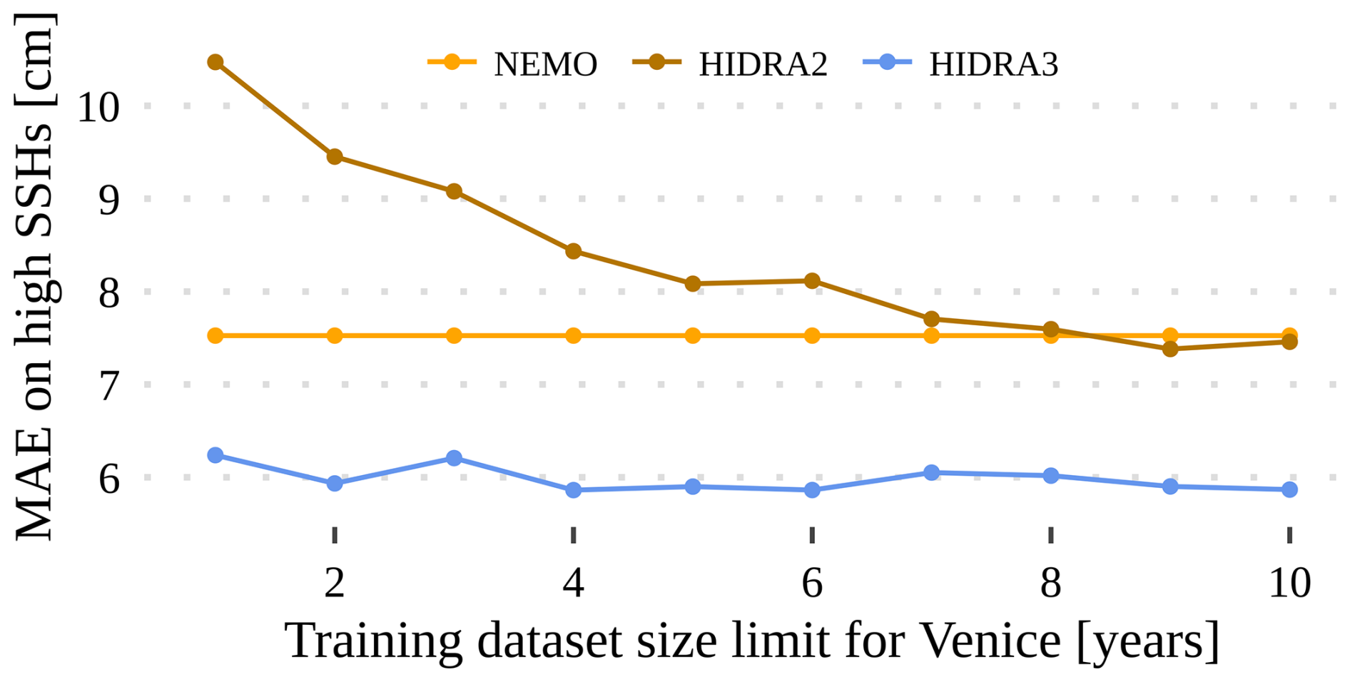
Figure 19 MAE on high SSH values when restricting training data in Venice to a maximum of 10 years. HIDRA3 achieves a substantially lower MAE than HIDRA2, particularly with limited historical training data.

3.6 Ablation study

3.6.1 Importance of considering multiple locations

To further analyze the proposed architecture, we retrained HIDRA3 at each location separately (ignoring all the others) and compared it using the same inputs as HIDRA2 – we refer to this variant as HIDRA3₁. The results in Table 4 and Fig. 20 show that, on average, HIDRA3₁ achieves a better performance than both HIDRA2 and NEMO in the overall metrics, with HIDRA3₁ in particular excelling on the high SSH values. HIDRA3₁ consistently outperforms HIDRA2 across all the locations, indicating the superiority of the proposed architecture even when it cannot exploit the information from multiple locations.

Multiple locations nevertheless substantially benefit the training process, as can be seen by comparing HIDRA3₁ to HIDRA3. The MAE of HIDRA3₁ is higher by 7.4 % and 6.9 % on high SSH values, meaning that observing multiple locations is beneficial to the overall performance and that HIDRA3 is able to leverage and combine the information from all the stations into a more accurate forecast.

Table 4 Performance of NEMO, HIDRA2, and HIDRA3₁, where HIDRA3₁ is the model trained separately on every single location. Bold values indicate the best performance in each part of the table.

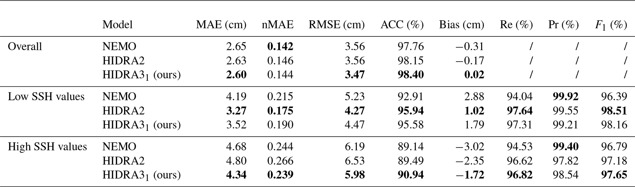
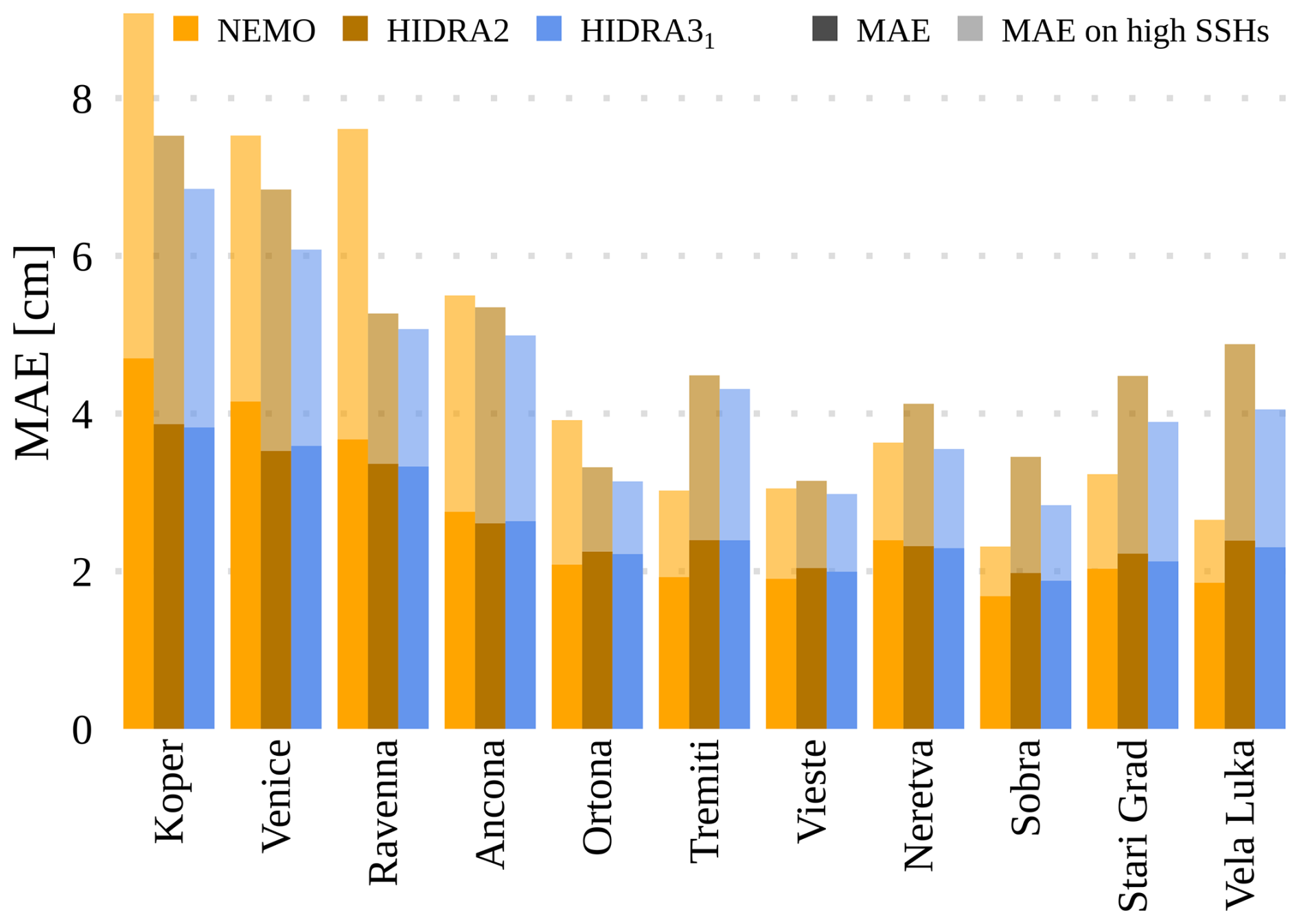
Figure 20 MAE comparison between the locations, where HIDRA3₁ is the model trained separately on every single location.

3.6.2 Impact of sea temperature and waves

To evaluate the importance of using sea surface temperature and wave data to enhance our model, we retrained HIDRA3 with these variables ablated. We first removed sea surface temperature only, which resulted in an average 1.7 % increase in the overall MAE and a 1.2 % increase in the MAE on high SSHs. Next, we removed wave data only, which led to an average 1.2 % increase in the overall MAE and a 2.4 % increase in the MAE on high SSHs. Finally, in the third experiment, we removed both sea surface temperature and wave data, which caused an average 0.8 % increase in the overall MAE and a 2.7 % increase in the MAE on high SSHs. These results suggest that sea surface temperature and wave data are not the main sources of HIDRA3's excellent performance. However, they do make a non-negligible contribution, and we recommend using them in the SSH prediction tasks.

3.6.3 Importance of the skip connection

Finally, we quantify the impact of passing the location-specific features x_i directly to the SSH regression module in addition to the fused features from the other locations, as shown in Fig. 4 in Sect. 2.2.3. For that, we change the SSH regression module so that it only accepts the fused features s and train the model by limiting the training data from Venice to 1 year. This setup was chosen to showcase the performance change in locations with fewer historical SSH measurements. In Sect. 3.5, we observe that HIDRA3 achieves a MAE on high SSH values of 6.24 cm, but with the changed architecture the MAE increases to 7.25 cm, which is an increase in the error of 16.2 %. This verifies our architectural design choice, which passes the location-specific features x_i to the SSH regression module in addition to the joint state, thus improving the location-specific information flow.

3.7 HIDRA3 limitations

HIDRA3 can generate forecasts for all the locations, even if the data from some of the locations are missing, which is a substantial improvement on its predecessor HIDRA2. The current implementation of HIDRA3 disregards the entire 72 h SSH dataset from the previous 3 d if even a single value of SSH is missing. This might be an overly stringent criterion, and we are working to find optimal ways of addressing this. Furthermore, in a highly unlikely situation where the sensors at all the locations fail and the data are missing for the full 72 h past period, HIDRA3 cannot generate forecasts reliably. In this case, a potential solution using the past HIDRA3 prediction as the input for the current prediction is still applicable. Preliminary simulations of such scenarios indicate that the MAE of HIDRA3 increases by 35 % overall and by 43 % for high SSH values. Additional work, however, needs to be done to further constrain HIDRA3 behavior in such scenarios.

4 Conclusions

We present HIDRA3, a new deep-learning architecture for multi-location sea level prediction with a temporal horizon spanning several days. Machine-learning models have recently emerged as a highly competitive alternative to general circulation models, but they are often challenged by the need for extensive periods of training data and operational reliance on real-time SSH observations, which may not always be available due to sensor failures. HIDRA3 addresses these challenges by being robust to individual and multiple tide gauge failures. This approach not only improves training where historical data are scarce but also enables predictions in the absence of real-time SSH data from a subset of training locations. HIDRA3 furthermore introduces a new reliable module for the estimation of prediction uncertainties, enhancing the interpretability of forecasts and their integration into downstream operational services.

In a challenging experimental setup, HIDRA3 outperforms both the current state-of-the-art deep-learning model HIDRA2 and the CMEMS version of the NEMO general circulation model. Results show excellent prediction capabilities even with limited training data, indicating a remarkable generalization capability of the proposed architecture.

The ability to exploit data from multiple locations for improved individual predictions, robustness to sensor failures, and uncertainty estimation capabilities makes HIDRA3 a powerful tool for coastal flood forecasting in regional basins with high variability in the availability of tide gauge data. Our future work will focus on densifying the prediction locations, ultimately leading to fully dense two-dimensional temporal predictions, which will further extend the application outreach of the HIDRA models.