Statistical summaries for streamed data from climate simulations: one-pass algorithms

Global climate models (GCMs) are being increasingly run at finer resolutions to better capture small-scale dynamics and reduce uncertainties associated with parameterizations. Despite advances in high-performance computing (HPC), the resulting terabyte- to petabyte-scale data volumes now being produced from GCMs are overwhelming traditional long-term storage. To address this, some climate modelling projects are adopting a method known as data streaming, where model output is transmitted directly to downstream data consumers (any user of climate model data, e.g. an impact model) during model runtime, eliminating the need to archive complete datasets. This paper introduces the One_Pass Python package (v0.8.0), which enables users to compute statistics on streamed GCM output via one-pass algorithms – computational techniques that sequentially process data in a single pass without requiring access to the full time series. Crucially, packaging these algorithms independently, rather than relying on standardized statistics from GCMs, provides flexibility for a diverse range of downstream data consumers and allows for integration into various HPC workflows. We present these algorithms for four different statistics: mean, standard deviation, percentiles and histograms. Each statistic is presented in the context of a use case, showing its application to a relevant variable. For statistics that can be represented by a single floating point value (i.e. mean, standard deviation, variance), the results are identical to “conventional” approaches within numerical precision limits, while the memory savings scale linearly with the period of time covered by the statistic. For statistics that require a distribution (percentiles and histograms), we make use of the t-digest, an algorithm that ingests streamed data and reduces them to a set of key clusters representing the distribution. Using this algorithm, we achieve excellent accuracy for variables with near-normal distributions (e.g. wind speed) and acceptable accuracy for skewed distributions such as precipitation. We also provide guidance on the best compression factor (the memory vs. accuracy trade-off) to use for each variable. We conclude by exploring the concept of convergence in streamed statistics, an essential factor for downstream applications such as bias-adjusting streamed data.

1 Introduction

Climate change impacts are often felt at the local level, where decision makers require timely and localized information to anticipate and develop necessary adaptation measures (Katopodis et al., 2021; Orr et al., 2021). Projections from regional and global climate models (RCMs and GCMs) are regularly used to create such information for climate adaptation policies and socio-economic decisions (Pörtner et al., 2022) but often lack the suitable spatial resolution and temporal frequency to be fully exploited. To support this need, RCMs and GCMs are being run at increasingly finer spatio-temporal resolutions, which can better resolve the smaller-scale dynamics of the Earth's climate system (Palmer, 2014; Bador et al., 2020; Iles et al., 2020; Stevens et al., 2020; Rackow et al., 2025). This ongoing movement in the climate community towards increasingly higher spatio-temporal resolutions raises the question as to how these data will be managed (Hu et al., 2018; Bauer et al., 2021). The growing size of the model output makes the current state-of-the-art archival method (e.g. Coordinated Regional Climate Downscaling Experiment (CORDEX) and Coupled Model Intercomparison Project (CMIP)) unfeasible. Moreover, the current archival method has left some data consumers without their required data, as climate model protocols either limit the number of variables stored or reduce their resolution and frequency (e.g. by storing monthly means or interpolated grids) to cope with the size. Here we refer to data consumers as external users who are not involved in the climate modelling process or diagnostics and traditionally access model output via static archives.

In this context, initiatives such as Destination Earth (DestinE) (Bauer et al., 2021; Hoffmann et al., 2023; Wedi et al., 2025) are utilizing a way to process the outputs of climate models as soon as they are produced, without having to save the full datasets to disc. This method, known as data streaming, transmits data in a continuous stream to data consumers, who can process them (e.g. via impact models) during runtime (Kolajo et al., 2019; Marinescu, 2023). The data stream allows those data consumers currently limited by reduced storage archives to access the full model output at the highest frequency available (e.g. hourly) and native spatial resolution. However, the advent of data streaming in the climate community poses its own set of challenges. Often, downstream data consumers require climate data that span long periods. For example, many hydrological impact models require daily, monthly or annual maximum precipitation values (Teutschbein and Seibert, 2012; Samaniego et al., 2019), while in the wind energy sector, accurate distribution functions of the wind speed are essential information (Pryor and Barthelmie, 2010; Lledó et al., 2019). Moreover, as all models are subject to systematic biases, many users require bias-adjusted climate data. Normally, these computations would be done using conventional methods, which require the entire dataset to be available when the computation is performed. In the streaming context, the one-pass problem is introduced: how to compute summaries, diagnostics or derived quantities without having access to the whole time series.

In this paper, we introduce the One_Pass package (v0.8.0), a flexible, bespoke Python package built to compute statistics and aid in the bias adjustment of streamed climate data using one-pass algorithms. While one-pass algorithms have been adopted in other fields such as online trading (Loveless et al., 2013) and machine learning (Min et al., 2022), they have yet to find a foothold in climate science, mainly because their use was not necessary, until now. Unlike the conventional method, one-pass algorithms do not have access to the whole time series; rather, they process data incrementally every time a climate model outputs new time steps (Muthukrishnan, 2005). This is done by sequentially processing data chunks as they become available, with each chunk's value being incorporated into a rolling summary, which is then moved into an output buffer before processing the next chunk. Details of the package's design choices – including its requirements for flexibility – and its current use in high-performance computing (HPC) workflows are given in Sect. 2. The remainder of the paper focuses on the mathematical theory behind the one-pass algorithms and investigates their utility and accuracy for climate data analysis. We do not discuss the code implementation; however, examples of the packages can be found in the provided Jupyter notebooks. In Sect. 3 we present the mathematical notation used throughout this paper. Sections 4 to 6 then cover the algorithms used for the mean, standard deviation and statistical distributions. These statistics have been chosen because they represent the most commonly required statistics for climate data, although many other statistics (i.e. minimum, maximum, threshold exceedance, etc.) have been implemented in the One_Pass package using the same approach. For each statistic, the one-pass algorithm is first presented, followed by an example use case which applies the algorithm to a relevant variable over a meaningful time span. With the aid of these use cases, the numerical accuracy is compared to the conventional approach (being able to read the dataset as a whole to compute the statistic), along with the achieved memory savings. In this paper, the conventional approach is always calculated with Python's NumPy package (Harris et al., 2020).

In Sect. 7 we discuss challenges that arise when using streamed data from one-pass algorithms for certain applications. For example, climate model outputs are often bias-adjusted using probability distribution functions (PDFs) to perform a quantile–quantile mapping against a reference dataset (Lange, 2019). The One_Pass package can be used to create these PDFs from the streamed data. However, these estimates will initially fluctuate and only converge as more data points are added. It is then crucial to know after how many samples the estimate (i.e. the PDF) is representative of the entire period – in other words, when it has converged. Only if convergence is attained can the PDF estimate be used for downstream applications (e.g. bias adjustment). Overall, the aim of this work is to both showcase the utility and highlight the current limitations of one-pass algorithms for climate data analysis. Moreover, through the provision of the One_Pass Python package, we show the foundations of the infrastructure required for the climate community to harness the capabilities of kilometre-scale climate data through data streaming.

2 Design and implementation in a workflow

The Climate Change Adaptation Digital Twin (ClimateDT) is one of the components of Destination Earth, a flagship initiative of the European Commission (Bauer et al., 2021; Hoffmann et al., 2023; Wedi et al., 2025). The ClimateDT aims to combine kilometre-scale global climate modelling with impact sector modelling in a single end-to-end workflow. One of the overarching aims is therefore to provide climate impact information tailored to different user needs by directly transforming climate model output. However, a gap often exists between the needs of specific data consumers and the general requirements of models. Moreover, the ClimateDT runs on several different HPC platforms, with several different GCMs. While many modelling groups will agree on providing monthly means via online calculations for specific variables (e.g. NOAA-GFDL, 2007), it is not realistic, nor feasible, for GCMs to tailor and maintain the disparate needs of data consumers from the impact modelling side. For instance, a data consumer focused on renewable energy production might be interested in monthly wind speed percentiles at a specific height in a particular location. The implementation of this output in climate models is impractical, whose goal is to provide outputs that are as general as possible. The development of the ClimateDT as a flexible, scalable framework emerges as a challenge in addition to that posed by the increase in spatio-temporal resolution. The One_Pass package was conceived in the frame of the ClimateDT to fulfil the requirements of downstream data consumers while keeping the model outputs relatively agnostic.

The data flow in the ClimateDT is orchestrated through a structured workflow that organizes a sequence of interdependent computational jobs. This workflow is managed using Autosubmit (Manubens-Gil et al., 2016), which automates the submission and monitoring of jobs on the target HPC platform. The One_Pass package runs as one of these jobs in the ClimateDT workflow, serving as an interface between the data production and its consumption. In this job, the One_Pass package operates via a central class Opa, which initially takes a request defined by the data consumer. The request primarily contains the information relevant to the aggregation of a variable. This information includes, among other things, the variable in question, the statistic to compute and the frequency of aggregation. Once this request is filed, and an instance of this class is created, the resulting object is set up to perform one-pass aggregations, taking in data chunks of arbitrary time length, which belong to the active streaming window. After performing a series of sanity checks on the incoming time steps, the instance of Opa updates its internal state to include the requested aggregation up to the time corresponding to the last incoming data chunk. Once enough data have been taken in to complete the requested statistic, the instance will output the requested variable aggregated at the specified frequency and move on to the next calculation.

Because the One_Pass package runs in an HPC environment, it is designed in a persistent manner. This means that the job in which it runs is not required to sit idly and consume HPC hours while there is no model output ready to process. This saves computing resources; however it does require the current status of the statistic to be saved between jobs. This is done via checkpointing, where each instance of the Opa class is stored after every update as a binary file. Similarly, upon initialization, it will load an existing state from a previous execution (if one exists) to use as a starting point. It will not store any internal state after the completion of the statistic. In the context of the ClimateDT, this is all handled by Autosubmit, the workflow manager, although the package can be used with other HPC workflow managers.

3 Mathematical notation

For a given dataset, the following mathematical notation is used to describe the one-pass algorithms:

• n is the current number of data samples (time steps) passed to the statistic.

• w is the length of the incoming data chunk (number of time steps).

• c is the number of time steps required to complete the statistic (i.e. if the model provides hourly output, and we require a daily statistic, c=24).

• x_n is one time step of the data at time t=n.

• ${\mathit{X}}_n=\mathit{\{}{x}_{\mathrm{1}},x_{\mathrm{2}},\mathrm{\dots },x_n\mathit{\}}$ represents the full dataset up to t=n.

• ${\mathit{X}}_w=\mathit{\{}{x}_{n+\mathrm{1}},\mathrm{\dots },x_{n+w}\mathit{\}}$ is the incoming data chunk of length w.

• S_n is the rolling summary of the statistic before the new chunk at time t=n. This summary varies for each statistic (i.e. if it is the mean statistic, $S_n={\overline{X}}_n$). This rolling summary will always be of length one in the time dimension.

• g is a one-pass function that updates the previous summary S_n with new incoming data X_w.

We introduce the chunk length w as, in many cases, an active data streaming window will contain a few consecutive time steps output from the climate model. In the case where the incoming data stream has only one time step, (w=1), X_w reduces to x_n+1.

4 Mean

4.1 Algorithm description

The one-pass algorithm for the mean is given by

$$\begin{array}{}\text{(1)}& {\overline{X}}_{n+w}=g(S_n,{\mathit{X}}_w)={\overline{X}}_n+w\left({\displaystyle \frac{{\overline{X}}_w-{\overline{X}}_n}{n+w}}\right),\end{array}$$

where ${\overline{X}}_{n+w}$ is the updated rolling mean of the dataset with the new data chunk X_w, and the rolling summary S_n is given by the rolling mean ${\overline{X}}_n$. If $w>\mathrm{1},{\overline{X}}_w$ is the temporal conventional mean over the incoming data chunk; however if the data are streamed at the same frequency of the model output with w=1, then ${\overline{X}}_w=x_{n+\mathrm{1}}$.

4.2 2 m air temperature

We apply the mean one-pass algorithm given in Eq. (1) for the analysis of 2 m air temperature data. European projects such as nextGEMS (Segura et al., 2025) and DestinationEarth (2024) are aiming to provide global climate projections for a variety of variables at spatial resolutions on the kilometre scale, ranging from 0.025 to 0.1°. This will allow for granular analysis of projected temperatures to inform climate adaptation at local to regional scales, although performing basic computations with such vast amounts of data can prove challenging. In this use case for the mean algorithm, we use data from the ECMWF's Integrated Forecasting System (IFS) model coupled with the Finite Element/Volume Sea-ice Ocean Model (FESOM) (tco2559-ng5-cycle3 experiment) (Koldunov et al., 2023; Rackow et al., 2025) (run as part of the nextGEMS project), looking at 2 m temperature in March 2020. We use hourly data at native model resolution (∼ 0.04°), resulting in a global map containing approximately 26.31 million spatial grid cells, 744 time steps and a full size of 145.82 GB with double precision (float64).

We calculated the March monthly mean of these data using both the conventional method and the one-pass algorithm given in Eq. (1). Computing the temporal conventional mean of these data requires the full time series to be loaded into memory, summed across every cell and then divided by the length of the time dimension (in this case 744). Due to the high memory requirements of this dataset, this was performed on a high-memory node (256 GB) on the Levante HPC system. The dataset was re-chunked into 10 spatial chunks using the Python library Dask-Xarray (Dask, 2024), where each chunk could fit into available memory. The conventional mean was then computed on each chunk. For the one-pass computation, we used a chunk length of w=1 and called into memory each hour x_n of the dataset to simulate streaming, iteratively updating Eq. (1) until n=c. These two methods highlight that with such large datasets, the conventional mean is not necessarily the simplest approach, as we still need specialized tools and high memory resources for computation. Rather than adding additional complexity, the one-pass approach allows for simpler handling and easier computation.

The results of the one-pass mean algorithm can be seen in Fig. 1a. We note that for plotting convenience, the native grid was interpolated to a 0.1° regular lat–long grid. Figure 1b shows the difference between the conventional (NumPy) and the one-pass mean shown in (a). The difference is represented by randomly distributed noise on the order of 10⁻¹², an accuracy within an insurmountable precision limit set by the machine precision as opposed to algorithmic discrepancies.

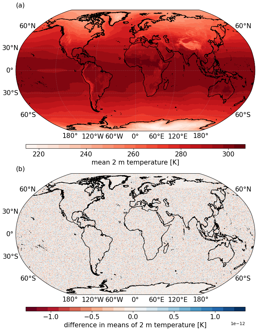
Figure 1 (a) Global monthly mean of 2 m temperature in March 2020 using hourly data from the IFS model, computed using the one-pass algorithm given in Eq. (1). (b) The difference between (a) and the mean calculated using the conventional method.

With regards to memory savings, the one-pass method requires only two data memory blocks, ${\overline{X}}_w$ and x_n, both approximately 200 MB with double precision (which is the size of one global time step), to be kept in memory at any point in time. If this computation was performed in real streaming mode, this would require only ∼ 400 MB of memory to compute the monthly mean, $\mathrm{2}/\mathrm{744}$th of the 145.82 GB memory requirements for the conventional method. We also note here that the memory cost of the one-pass method is independent of the length of the statistic time span. For the case of w=1, the memory requirements will always be twice that of storing a spatial field, as opposed to the conventional method, where the memory requirements will increase linearly with the length of the time series required to compute the statistic. Moreover, this computation demonstrates that the one-pass algorithms do not merely provide memory savings; they provide user-oriented diagnostics that allow for easy computation. Due to this vast reduction in memory requirements, different variables can be computed in parallel to each other, further enhancing usability. The current paradigm of loading the entire dataset is not practical (and in some cases not possible) for data of this magnitude. Indeed, special tools such as Python's Dask-Xarray packages are often required.

5 Standard deviation

5.1 Algorithm description

The one-pass algorithm for the standard deviation (and also variance) is calculated over the requested temporal frequency c by updating two estimates iteratively: the one-pass mean and the sum of the squared differences. First, let the conventional summary for the sum of the squared differences, M_c, be defined as

$$\begin{array}{}\text{(2)}& M_c=\sum _{n=\mathrm{1}}^c(x_n-{\overline{X}}_c{)}^{\mathrm{2}},\end{array}$$

where ${\overline{X}}_c$ is the conventional mean of the whole dataset X_c required for the statistic. For the one-pass calculation of the standard deviation, the rolling summary S_n defines the sum of the squared differences, M_n. In the case where w=1, the rolling summary is updated by

$$\begin{array}{}\text{(3)}& \begin{array}{rl}{M}_{n+\mathrm{1}}& =g(S_n,x_{n+\mathrm{1}})\\ & =M_n+(x_{n+\mathrm{1}}-{\overline{X}}_n)(x_{n+\mathrm{1}}-{\overline{X}}_{n+\mathrm{1}}),\end{array}\end{array}$$

where ${\overline{X}}_n$ and ${\overline{X}}_{n+\mathrm{1}}$ are both given by the algorithm for the one-pass mean in Eq. (1). Equation (3) is known as Welford's algorithm. In the case where the incoming data have more than one time step (w>1), M_n is updated by

$$\begin{array}{}\text{(4)}& \begin{array}{rl}{M}_{n+w}& =g(S_n,{\mathit{X}}_w)\\ & =M_n+M_w+{\displaystyle \frac{wn({\overline{X}}_n-{\overline{X}}_w{)}^{\mathrm{2}}}{n+w}},\end{array}\end{array}$$

where M_w is the conventional sum of the squared differences over the incoming data block of length w (given by Eq. (2) with c=w), ${\overline{X}}_n$ is the one-pass mean at t=n calculated with Eq. (1), and ${\overline{X}}_w$ is the conventional mean of the incoming data block. See Mastelini and de Carvalho (2021) for details.

Once enough data have been added to the rolling summary M_n so that n=c we calculate the standard deviation σ using

$$\begin{array}{}\text{(5)}& \mathit{\sigma }=\sqrt{{\displaystyle \frac{M_n}{n-\mathrm{1}}}},\end{array}$$

to obtain the sample variance. Equation (5) also applies to the conventional summary M_c.

5.2 Sea surface height variability

We apply the one-pass algorithm for standard deviation to the sea surface height (SSH). The standard deviation of SSH can be used to quantify uncertainty between different model ensembles compared to satellite altimetry data. The SSH can be used to better understand ocean dynamics as its variability gives insights into the redistribution of mass, heat and salt within the water column (Close et al., 2020). We calculate the annual standard deviation using data from the FESOM model (tco2559-ng5-cycle3 experiment) (Rackow et al., 2025), again run as part of the nextGEMS project. We use daily data over 2021 at native model resolution (∼ 0.05°), making an annual time series – comprised of 7.4 million grid cells and 365 time slices – of 10.09 GB using single precision (float32). We first calculate the standard deviation using the conventional method defined in Eq. (2), followed by the one-pass method in Eq. (4), with w=2. Like with the mean calculation, for the conventional calculation the data were spatially re-chunked into 10 chunks using the Python library Dask-Xarray, and each chunk was computed separately, while for the one-pass, two daily time steps were iteratively called into memory to simulate data streaming.

Figure 2a shows the one-pass standard deviation calculated using Eqs. (4) and (5) (using the One_Pass package; see notebooks). Figure 2b then shows the difference between the one-pass and the conventional calculation. Again, for plotting convenience, the native grid was interpolated to a 0.25° regular lat–long grid. Here, the order of magnitude of the difference is 10⁻¹⁶, even smaller compared with the mean difference in Fig. 1b. Interestingly, we also see some structure emerging in the differences shown in Fig. 2b, which correlates with areas of larger standard deviation. However, due to the extremely small values, it is considered negligible in comparison to the required accuracy of the statistic. Therefore, as with the mean statistic, this difference can also be attributed to machine precision limitations.

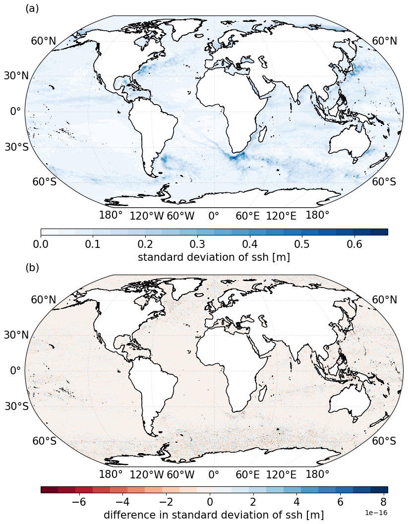
Figure 2 (a) Global annual standard deviation of the sea surface height in 2021 using daily data from the FESOM model, computed using the one-pass method given in Eqs. (4) and (5), implemented with the One_Pass package. (b) The difference between the one-pass computation and the conventional computation.

The memory savings for the standard deviation are slightly inferior to the mean one-pass algorithm as here, in the case of w>1, other than the current data memory block X_w, four additional data summaries are required to be kept in memory: M_n, M_w, ${\overline{X}}_n$, ${\overline{X}}_w$. However, as with the mean, these memory requirements are independent of the time span (sample size) of the statistic and do not increase as the number of values required to complete the statistic (c) increases. In the example presented here, with w=2, approximately 112 MB of memory (single precision) is required, as opposed to the 10.09 GB of the full dataset. This is a reduction of 2 orders of magnitude in memory requirements.

6 Distributions: percentiles and histograms

6.1 Algorithm description

Unlike the one-pass algorithms for mean and standard deviation (and others such as minimum, maximum, threshold exceedance), where the rolling summary S_n can be described by one floating point value, estimates of a distribution cannot be condensed in such a way. The t-digest algorithm, developed by Dunning and Ertl (2019) and Dunning (2021), creates reliable estimates of PDFs with a single pass through the dataset. The t-digest algorithm is used here, to the best of our knowledge, for the first time in climate data analysis. Our One_Pass package (and all the results presented in Sect. 6) uses the Python package crick (Crist-Harif, 2023) for the implementation of the t-digest algorithm. We note that other packages may provide slightly different results and efficiency due to variations in the algorithm implementation; however, our preliminary analysis conducted when investigating different packages did not show these to be substantial.

The t-digest algorithm represents a dataset X_n by a series of clusters that are defined by their arithmetic mean value and their corresponding weight (i.e. the number of samples that have contributed to the cluster/mean). For streamed data, each value (x_n) is added to its nearest cluster, based on the value's proximity to the cluster's mean. As x_n is added, the weight and mean of that cluster are updated using Eq. (1). The clusters are organized in such a way that those corresponding to the extremes of the distribution will contain fewer samples than those around the median quantile, meaning that the error is relative to the quantile, as opposed to a constant absolute error seen in previous methods (Dunning and Ertl, 2019). The unequal sizes (i.e. the weights) of these clusters are set by the monotonically increasing scale function. While there is a range of possible scale functions, here we use the most common,

$$\begin{array}{}\text{(6)}& k\left(q\right)={\displaystyle \frac{\mathit{\delta }}{\mathrm{2}\mathit{\pi }}}{\text{sin}}^{-\mathrm{1}}(\mathrm{2}q-\mathrm{1}),\end{array}$$

where q is the quantile, and δ is the compression parameter. Figure 3a provides a visual representation of the scale function in Eq. (6) for four different δ values (also see Fig. 1 in Dunning and Ertl, 2019). Regardless of the compression parameter, there is a steeper gradient of k near q=0 and q=1. As the size of a given cluster is determined by the slope of k, this steeper gradient reduces the cluster weights over the tails of the distribution. For mathematical details of how the cluster sizes are determined, see Dunning and Ertl (2019). The compression parameter does not affect the shape of the scale function, but it does increase the range of k. The greater the range of k, the more clusters will be used to represent X_n, providing more accuracy but also increasing the memory required. This is demonstrated by the shaded grey dots in Fig. 3a, located on the lines for δ=20 and δ=100. The number of dots shows the number of clusters used to represent a dataset X₅₀₀, while the size of the dot indicates the weight. Significantly fewer clusters are used for δ=20 compared to δ=100, reducing the accuracy along with the memory requirements. These clusters are ultimately converted to a percentile or a histogram (where bin densities may have non-integer values due to the underlying cluster representation), based on the closest cluster mean to the required percentile.

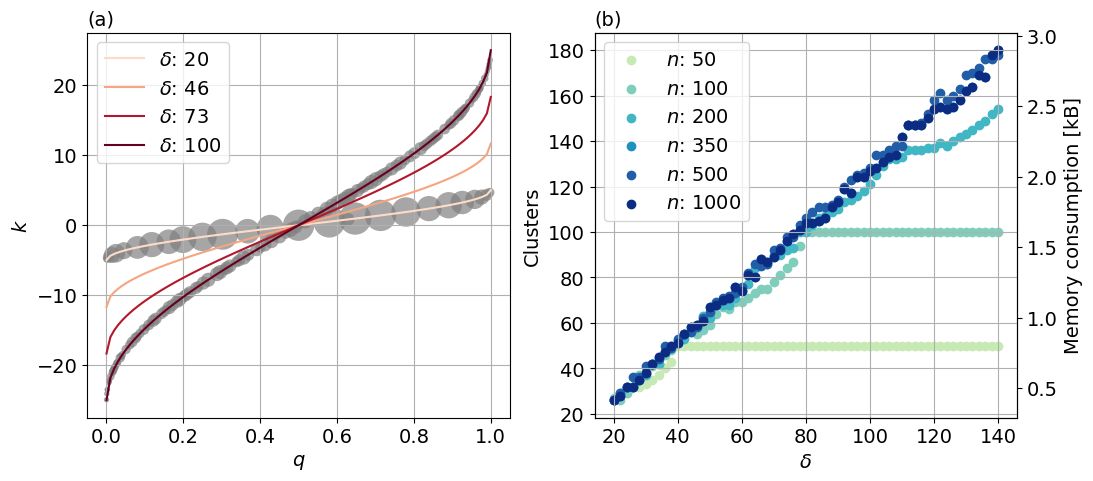
Figure 3 (a) Graphical representation of the scale function in Eq. (6) for four different δ values. The grey dots for δ=20 and δ=100 show the clusters that would be used to represent a dataset of n=500, with a mean value and associated quantile (q) and a weight represented by the size of the dot. (b) Number of clusters used to represent datasets of varying lengths as a function of the compression parameter δ. The corresponding memory consumption [kB] is given on the right-hand axis. Six random datasets (sampled from a uniform distribution) of lengths ranging from 50 to 1000 are used.

The effect of the compression parameter δ on the memory requirements is shown in Fig. 3b, while the effects on accuracy of the percentile estimates are given in Sect. 6.2 and 6.3. In Fig. 3b, six random datasets (from a uniform distribution) of different lengths (n) are used to show how many clusters are required to represent the data as a function of δ (within the range 20 $\le \mathit{\delta }\le$ 140). Beyond n>350, shown by the darkest three samples, the number of clusters used to represent the data grows linearly with δ. This means that, for the range of δ tested, for all datasets with more than 350 values, the number of clusters is independent of the size of the dataset and is set only by δ; i.e. a dataset of 500 values will be represented with the same number of clusters as a dataset of 5 million values. For smaller dataset sizes (anything below 350, as shown by the three lighter blue/green samples in Fig. 3b) there may be no memory savings (depending on δ) generated from using the algorithm, as each cluster requires two values (mean and weight) for its representation. For example, when considering δ=140 and a sample size of 350, 180 clusters are used, requiring 360 values, which exceeds the length of the original dataset. Indeed, for very short datasets such as n=50 (lightest green line in Fig. 3b), the number of clusters cannot grow beyond 50 as the distribution is already represented in its entirety, with each cluster containing one data sample with a weight of one. For these shorter datasets, there will be no added benefit of increasing δ. However, for longer sample sizes and/or smaller δ, the memory savings generated are substantial.

In Sects. 6.2 and 6.3, we examine the use of the t-digest algorithm with two case studies: wind energy in Sect. 6.2 and extreme precipitation events in Sect. 6.3. These two examples have been chosen to examine how well the t-digest algorithm represents (a) a more normally distributed variable around the median percentiles and (b) extreme events at the tails of a heavily skewed distribution. Comparisons are made against the conventional method, calculated with NumPy, which has access to the full dataset and does not rely on one-pass methods. For the t-digest method, we used w=1 in both examples, meaning each x_n was added to its respective digest consecutively, to simulate data streaming.

6.2 Wind energy

We present here the application of the t-digest in the context of wind energy. With the decarbonization of the energy system turning into a global necessity, renewable energies such as solar and wind are becoming major contributors to the power network (Jansen et al., 2020). However, unlike with fossil fuels, wind energy production is heavily affected by atmospheric conditions, subject to both short-term variability (i.e. weather) and longer-term variations caused by seasonal and/or interannual variability (Grams et al., 2017; Staffell and Pfenninger, 2018). This volatility makes the integration of wind energy into the power network a challenging task (Jurasz et al., 2022).

Having access to histograms of wind speed from high-frequency data (i.e. at hourly or sub-hourly scale) and at hub height (i.e. height of the turbine rotor) is among the requirements of wind farm operators and stakeholders to estimate the available wind resources at a particular location. This information can be combined with the power curve of the turbines installed at each location to give reasonable estimates of energy production over a period of time. Obtaining an accurate representation of the wind distribution is therefore crucial, as the distributions condense the information from climate simulations required by the wind energy industry and aid in both the understanding of future output from current farms and in the decision-making relating to the viability of a proposed wind farm location (Lledó et al., 2019). Currently, there are two main methods for describing wind speed distributions: through full histograms of time series data or through fitting probability distribution functions to the data (Morgan et al., 2011; Shi et al., 2021). While the non-parametric approach (time series) generally outperforms the parametric (statistical) one in accurately characterizing the distribution (Wang et al., 2016), it poses numerous challenges attributable to the large amounts of data required (Shi et al., 2021).

We investigate the use of the t-digest algorithm to estimate the wind speed distribution from streamed climate data. We again use data from the ECMWF's IFS model (tco2559-ng5-cycle3 experiment), this time looking at the 10 m wind speeds over December 2020. We again use the hourly data at native model resolution (∼ 0.04°), resulting in a global map containing approximately 26.31 million spatial grid cells, 744 time steps and a full size of 145.82 GB with double precision (float64). However, for plotting convenience and storing in Zenodo (Grayson, 2024), the data have been spatially regridded to 1°. Wind speed is calculated from the root of the sum of the squares of the 10 m hourly mean zonal and meridional components. We conduct a detailed analysis of two locations, the offshore Moray East wind farm, located at (58.25° N, 2.75° E) in the North Sea, and the onshore Roscoe wind farm, positioned at (32.35° N, 100.45° W) in Texas. Both are marked on the global map in Fig. 4a in red and pink, respectively.

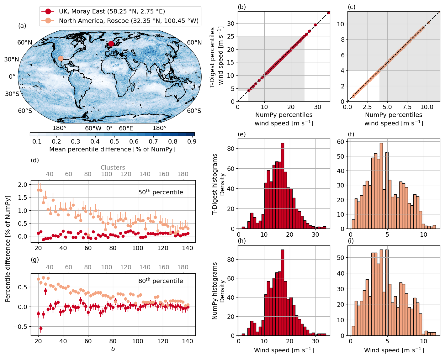
Figure 4 (a) Global map showing the absolute mean difference between the t-digest (δ=60) and NumPy (using the linear interpolation method) estimate of all wind speed percentiles from 1 to 100 given as a percentage of the NumPy value. Wind speed hourly data in December 2020 from the IFS model. The red dot marks the offshore Moray East wind farm in the North Sea (58.25° N, 2.75° E) and the pink dot the onshore wind farm in Roscoe, Texas (32.35° N, 100.45° W). (b) Quantile–quantile plot for percentiles 1 to 100 comparing NumPy and the t-digest algorithm (with δ=60) for Moray East. The dashed black line represents the one-to-one fit, while the shaded grey area shows the range of wind speeds that most commonly used turbines operate in Lledó et al. (2019). (c) Same as (b) but for the Roscoe wind farm. (e, h) Histograms of the Moray East time series, (e) calculated with the t-digest (δ=60) and (h) NumPy. (f, i) Same as (e), (h) but for the Roscoe time series. (d) The difference between the t-digest and NumPy calculation of the 50th percentile, given as a percentage of the NumPy value, as a function of δ for both marked locations. The error bars show the possible differences when employing all available NumPy interpolation schemes rather than the default linear interpolation method. (g) The same as (d) but for the 80th percentile.

Figure 4 shows a detailed comparison between how the t-digest and the conventional method describe typical wind speed distributions. Figure 4b and c show quantile–quantile plots for the NumPy percentile estimates against the t-digest estimates (using δ=60) for all percentiles ranging from 1 to 100 for (b) the Moray East wind farm time series and (c) the Roscoe time series. The shaded grey areas indicate the range of wind speeds in which most commonly used turbine classes operate (Lledó et al., 2019). For the offshore Moray East, the extreme maximum percentiles lie outside the grey shaded region, but the lower tail is within it, whereas for the on-shore Roscoe farm, the opposite is true. This shows that an accurate representation of the full wind speed distribution is required in order to cover the typical range of wind speeds relevant to wind farms. Both (b) and (c) show an almost perfect linear relationship, evidencing that the t-digest method provides the same level of accuracy as NumPy for typical wind speed distributions. This is further shown in (e), (f), (h) and (i), where the histograms of the distributions for the two locations are given using the t-digest method (e,f) and NumPy (h,i). The difference between the distributions provided by the two methods is minimal, with their main difference lying in the storage requirements. For the NumPy estimate, 5.95 kB is needed to store the full 744 value time series of one grid cell, compared to the 1.28 kB storage for the t-digest estimate based on 80 clusters (δ=60).

To ensure that the minor differences shown in Fig. 4b and c are not specific to the two chosen locations, we calculated the absolute mean percentile difference (average across all percentile estimates from 1 to 100, i.e. over the quantile–quantile plots) for every global grid cell for δ=60, the results of which are shown in Fig. 4a. In this global map, no difference exceeds 0.9 % of the NumPy value. Converting to actual terms, this translates to no absolute mean difference exceeding 0.068 m s⁻¹ across the globe. Taking the global spatial average of these mean differences gives 0.020 m s⁻¹.

Given such a high level of accuracy achieved with δ=60, we further investigate the effects of compression in Fig. 4d and g. For the same two locations, the difference in the estimate of the 50th and 80th percentiles between the two methods is shown as a function of δ. The difference is represented as a percentage of the NumPy percentile estimate, calculated using the default linear interpolation method. The error bars represent the range of possible differences between the t-digest and the NumPy estimates obtained from using the eight different interpolation schemes available in NumPy. The difference between the interpolation schemes, outlined in Hyndman and Fan (1996), will be larger for a given percentile estimate if the data points are more sparsely distributed in the original dataset. Therefore, when any type of interpolation is required to estimate a percentile, there will always be a range of possible values depending on the interpolation method chosen. We see that the difference for the Roscoe wind farm in Texas, while incredibly small, is slightly higher for both the 50th and 80th percentiles. This is due to the shape of the two distributions, as evident in the histograms in (f) and (i). Although the Moray East dataset has a larger variance, it more closely resembles a normal distribution, whereas the dataset for Roscoe is more uniform, with the peak skewed to the left. The shape of the scale function given in Eq. (6) will result in clusters with the lowest weight representing the distribution tails, while the clusters representing the middle of the distribution will have a larger weight. This is a clever characteristic of the algorithm, as due to the bulk of the data in a normal distribution being centred around the median, these middle clusters can afford to be larger and cover a broader range of values without impacting precision. As the data from the Roscoe site slightly deviate from this normal distribution, a small increase in the difference is observed.

However, despite this perceived higher difference for the Roscoe wind farm in Texas, the absolute maximum differences for both the 50th and 80th percentiles are approximately 2 % and 0.6 %, respectively, for the lowest compression factor, further decreasing as we increase δ. In actual terms, the maximum differences (for δ=20) are 0.075 and 0.1 m s⁻¹, respectively, errors which would be considered negligible for the end users. Moreover, while the 50th-percentile estimate at the Roscoe wind farm has the largest differences across all compression factors (light-pink data in (d)), it also has the largest error bars, indicating that the conventional method also contains greater uncertainty. This highlights that the different interpolation methods used by NumPy have a greater impact on the given result due to the sparser data, also explaining why the discrepancy between the one-pass and conventional methods is higher for this percentile estimate. We also observe an asymptote in the differences around δ=60 in Fig. 4d and g, showing that further increasing the compression parameter would not significantly enhance the accuracy of the results for these wind speed distributions. Indeed, given the extremely small calculated difference, using a δ= 40 would likely be sufficient to capture the distribution of global wind speed data required for users.

Overall, as wind speed is best described by a bi-modal Weibull distribution (Morgan et al., 2011), for monthly wind speed data at hourly time steps, the t-digest with δ=60 is more than suitable to fully represent the overall distribution while reducing the overall size of the global monthly data from 145.82 to ∼ 33.2 GB. At the grid cell level, the monthly time series is compressed from 5.9 to 1.2 kB. For δ=40, this would further reduce to 0.85 kB. We further note that if we were interested in time series longer than the month shown here – for example, annually – the hourly time series for one grid cell would require 8760 values (∼ 70 kB), while its representation with the t-digest would still only require 1.2 kB. In contrast, if our interest were in weekly datasets with a time step of 1 h, containing only 168 values (∼ 1.3 kB), using δ=60 would still require 1.2 kB. Although no significant memory savings would be obtained, the histograms could still be provided in real time to the users due to the data streaming.

6.3 Precipitation

In the following section we focus on the t-digest algorithm in the context of extreme precipitation events. It is necessary to examine these extreme events, such as intense rainfall and potential flood risk, as they pose great social, economic and environmental threats. Both theory and evidence are showing that anthropogenic climate change is increasing the risk of such extreme events, especially in areas with high moisture availability and during tropical monsoon seasons (Gimeno et al., 2022; Thober et al., 2018; Donat et al., 2016; Asadieh and Krakauer, 2015). The need for climate adaptation measures in vulnerable communities exposed to these risks is pressing, and, as with the other use cases in this paper, an accurate representation of the hazard is essential. Consequently, our focus here is on assessing how accurately the t-digest algorithm captures extreme events associated with the upper tail of precipitation distributions. In this analysis, we use data from the ICOsahedral Non-hydrostatic (ICON) model (Jungclaus et al., 2022; Hohenegger et al., 2023) (ngc2009 experiment), looking at precipitation over August 2021. We use half-hourly data using the Healpix spatial grid (Gorski et al., 2005) (∼ 0.04°) containing 20.9 million grid cells. The full monthly dataset for this variable, containing 1488 time steps, requires 116.25 GB of memory using single precision (float32). As with Sect. 6.2, for plotting convenience and storing in Zenodo (Grayson, 2024), the data have been spatially regridded to 1°.

Figure 5a–c illustrates the comparison between NumPy and the t-digest in their estimates of the 99th percentile of a precipitation distribution. We focus on four specific locations, each characterized by different distributions, with the locations in Brazil and the North Pacific specifically chosen to highlight the areas of largest discrepancy between the one-pass and conventional methods. The histograms in Fig. 5d–k show the full distributions for the four locations, with (d–e) created using the t-digest and (h–k) using NumPy. A common theme among precipitation distributions is that they are heavily skewed, with the majority of the data falling around zero when there is very little to no precipitation. The dark-red histograms in (d, h) are for the location in Brazil and show an extremely dry month with almost all of the values in the 0–1 mm d⁻¹ bin (notice the logarithmic scale). In contrast, the location in Columbia (e, i) reveals heavy precipitation over the month with maximum values above 400 mm d⁻¹ and a more even spread across the distribution. Despite the ranges in maximum values, all the t-digest histograms show a non-integer number of samples in some of the histogram bins, whereas the NumPy counterparts show integer density values, representing the exact values in the distribution. These non-integer values are due to a weighted contribution from the clusters to the histogram.

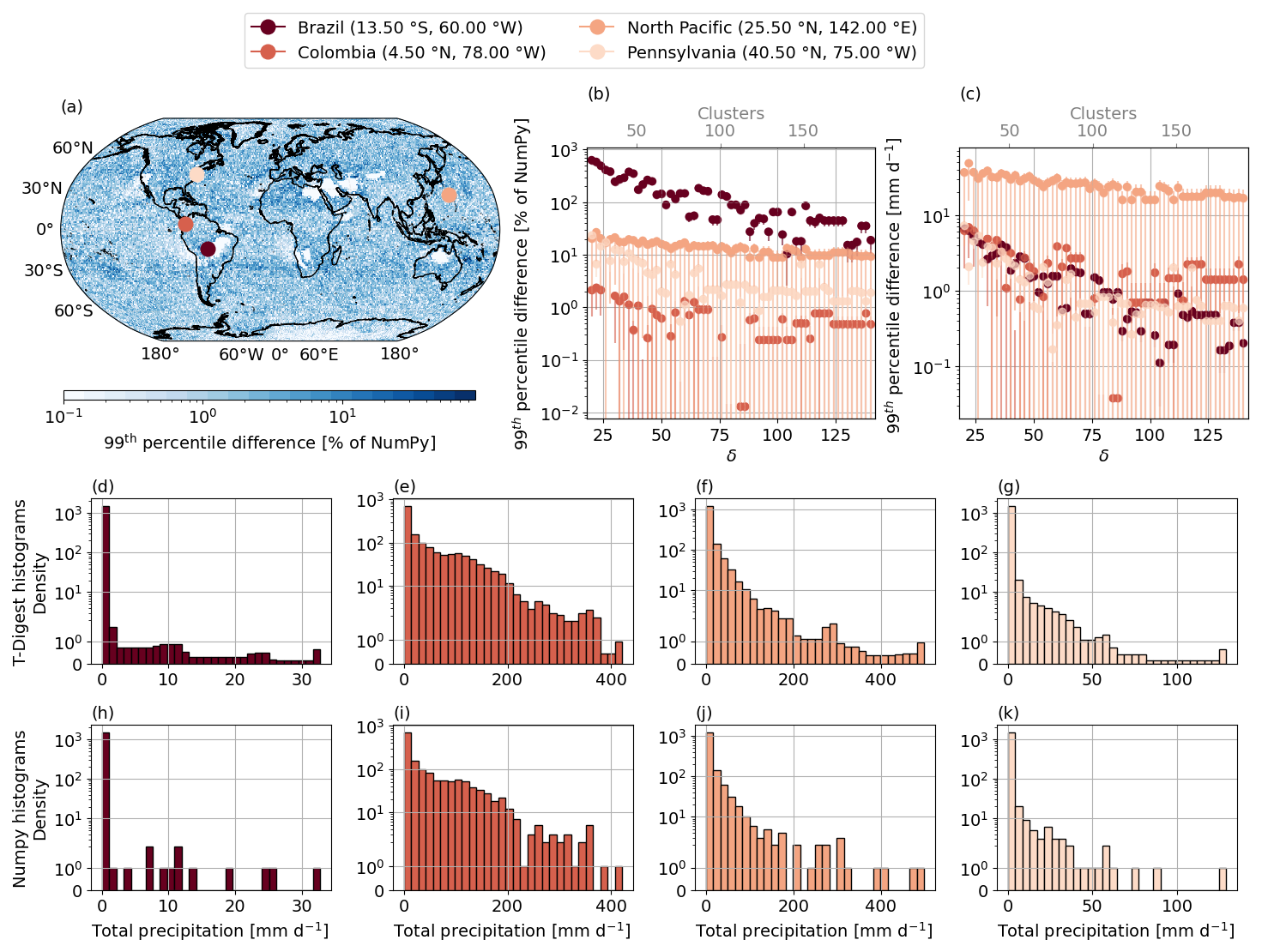
Figure 5 (a) The global map shows the absolute difference between the t-digest (δ=80) and NumPy (using the linear interpolation method) estimate of the 99th precipitation percentile given as a percentage of the NumPy value (see text for details). Half-hourly precipitation data from the ICON model (ngc2009 experiment) in August 2021 are used in each panel. The location of the four solid pink circles is given in the legend, and the following panels use the same colours to indicate the locations. (b) The absolute difference between the NumPy and t-digest 99th-percentile estimate, given as a percentage of the NumPy estimate, shown as a function of compression for the four marked locations in (a). The upper grey axis shows the number of clusters used in each digest for each δ. The error bars represent the range of possible differences based on all available NumPy interpolation schemes, in contrast to the default linear interpolation method (see text for details). (c) Same as (b) but given as the actual difference in mm d⁻¹. (d–g) Histograms calculated using the t-digest algorithm, with δ=80 showing the distribution of the total precipitation (mm d⁻¹) for each location. (h–k) Same as (d)–(g) but calculated using NumPy.

Figure 5c shows the difference between the NumPy and t-digest estimate of the 99th percentile for the total precipitation as a function of δ. The corresponding number of clusters for each δ is indicated in grey along the upper axis. Here the North Pacific location shows the greatest difference in the 99th-percentile estimate. The reason for this is clear when examining the corresponding histograms for the t-digest (f) and NumPy (j). Focusing on the NumPy histogram (the actual distribution) at the upper end, the data are sparse, with only four values in the top quartile of the data range. Due to this sparseness, the 99th-percentile estimate falls in between two data points, so the interpolation method used by NumPy significantly impacts the estimate. This is reflected in the error bars for the North Pacific location in Fig. 5c. While the difference between the t-digest and the NumPy estimate using linear interpolation is large (dots), other NumPy interpolation schemes result in a negative difference (not shown due to the logarithmic scale), showing that the t-digest estimate lies in between the different estimates obtained with the available NumPy interpolation schemes. These larger differences can therefore be better attributed to the low density of values at the upper tails as opposed to poor representation of these tails by the t-digest. While the location in Colombia also has a high range of values, as there are more samples in the upper tail of the distribution, the t-digest and NumPy estimates are more similar. As seen in Sect. 6.2, there is also a decrease in differences as δ increases.

Figure 5b shows the same differences presented in Fig. 5c but given as an absolute percentage of the NumPy estimate. Here, the largest error is seen for the location in Brazil. The reason for this large error is similar to the results in (c), where the sparseness of the data in other bins greater than 0–1 mm d⁻¹ is obvious in the NumPy histogram (h). However, as this area is so dry and the distribution so skewed, around 99 % of the data lie in the first bin, and the 99th-percentile estimate is 0.06 and 1.02 mm d⁻¹ for NumPy and the t-digest (δ=80), respectively. This highlights the challenges of working with precipitation values below 1, as percentage errors can show unrealistically poor results. To account for these unrealistically poor estimates we calculated the percentage difference for both Fig. 5a and b using $\text{error}=\mathrm{100}\left|\right(a-b\left)\right|/(b+\mathit{ϵ})$, where a is the t-digest estimate, b is the NumPy estimate using the linear interpolation (other than the error bars in Fig. 5b), and ϵ=1. This small constant ϵ is introduced to stabilize the calculation when b is extremely small. The results are shown globally (using δ=80) in Fig. 5a. Most of the differences fall between 1 % and 10 % of the NumPy value. However, due to the reasons just described, drier regions show larger percentage errors. Indeed, larger values are seen around the Saharan desert and in regions of eastern Australia. The average of the global differences is shown in Table 1 as a function of δ, given as both the percentile estimate and the absolute value. We have included this table to highlight that, due to the extremely low precipitation values for some of the estimates, a higher percentage difference does not necessarily translate to a higher difference in actual terms. Even with a relatively small δ of 40, the overall relative difference of the 99th percentile (when averaged globally) is less than 4 % (difference of 1.27 mm d⁻¹). Both of these differences decrease to less than 2 % and 0.60 mm d⁻¹ as δ increases to 120.

Table 1 Global average of the 99th percentile difference for different compression values, given as both the absolute difference in (mm d⁻¹) and as a percentage.

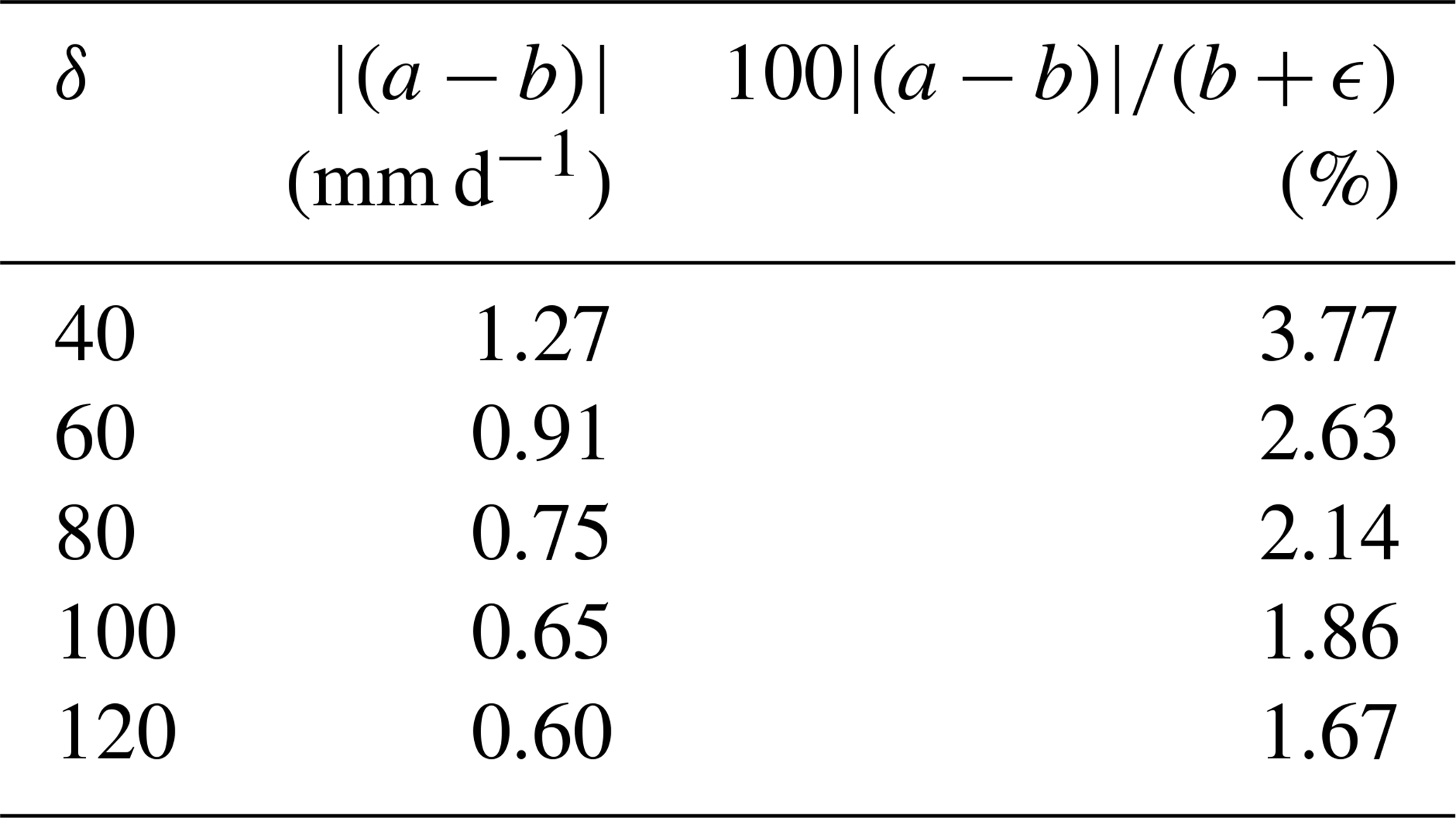
Based on the results from Table 1 and Fig. 5b and c we see a reduction in difference with increasing compression that asymptotes around δ≈ 80. This is higher than the asymptotic value seen in Fig. 4d and g of approximately δ≈ 60. In general, there are no significant accuracy improvements from using a δ more than approximately 80 (100 clusters) to represent the precipitation distributions, and we would not recommend exceeding this compression factor. Indeed, depending on the specific accuracy requirements, it may be beneficial to reduce this even further. Based on results from δ=80, the entire dataset of 116.25 GB could be represented with 36.57 GB, reducing the memory requirements by approximately a third.

One interesting point to raise is how the scale function for the t-digest algorithm, given in Eq. (6), impacts these results. While the differences obtained for the precipitation distributions are well within the acceptable limits for most use cases, comparing them with the results in Sect. 6.2, we see poorer accuracy. This is due to the wind distributions more closely resembling a normal distribution, which is the distribution that the symmetric scale function describes best. While outside the scope of this investigation, we note that to better represent these skewed precipitation distributions, a non-symmetric scale function that would create larger clusters at the lower tail may more accurately capture the underlying distribution. Another method to improve the representation of the dataset would be to simply impose a cut-off (such as 1 mm d⁻¹) for the data that are added to the digests. Removing this extremely large cluster close to zero would, in many cases, improve the representation of the data by the t-digest.

7 Convergence

While earlier sections focused on the accuracy and efficiency of one-pass algorithms for computing statistics, the broader goal of the One_Pass package is to support flexible, real-time analysis of streamed climate data. Beyond statistics, it also integrates with a companion Python package (not detailed here) designed for performing bias adjustment on streamed model output. Typically, bias adjustment uses quantile–quantile (Q–Q) mapping (Lange, 2019) to correct statistical biases. The t-digest algorithm is used to construct a dynamic distribution that enables the bias adjustment on streamed data. However, Q–Q mapping requires a stable and well-sampled distribution (S_n) of the model variable to function effectively. How to determine this leads to the vital question of how long the data stream needs to run for the statistic summary S_n to stabilize. We determine this based on the statistical summary's convergence rate (Grau-Sánchez et al., 2010).

The convergence rate is used in numerical analysis to determine how long a sequence of computations needs to run before reaching asymptotic behaviour. In the context of streamed climate data, this means that the statistic is not only representative of the data seen so far but also stable enough to reflect long-term behaviour. Taking the mean temperature as an example, at the beginning of a time series, the mean may change significantly with each new data point, but as more data accumulate, the changes diminish, signalling that convergence has been reached. Our intent is not to suggest that climate variables become stationary or stop evolving; rather, we aim to determine when the rolling estimate of a one-pass statistic summary S_n has stabilized sufficiently to be used confidently for subsequent statistical calculations such as bias adjustment. Moreover, this analysis does not contradict the earlier benefits of one-pass methods (e.g. reduced memory usage, early access to useful summaries). Rather, it offers guidance on how the rolling summaries can be used when n≠c and how soon those summaries can be used for bias adjustment or similar post-processing steps.

This concept of convergence is explored by examining the rolling summary S_n for 2 m temperature, 10 m wind speed, and precipitation from the IFS and ICON models. The temperature and wind speed datasets are the same IFS datasets used in Sects. 4 and 6.2, respectively, and the precipitation dataset consists of the same ICON data used in Sect. 6.3. For both temperature and wind speed the rolling summary $S_n={\overline{X}}_n$, while for precipitation S_n is the rolling 50th-percentile estimate. For all rolling summaries w=1, meaning that the number of samples, n, contributing to S_n grows by one each time. Unlike in the previous sections, where we were interested in the value of S_n at n=c, here S_n is stored at every time step, providing a time series of its development denoted as ${\mathit{S}}_n=\mathit{\{}{S}_{\mathrm{1}},S_{\mathrm{2}},\mathrm{\dots },S_n\mathit{\}}$. The rolling standard deviation (σ) is then taken of S_n using Eqs. (4) and (5). This results in a time series of σ defined as ${\mathit{\sigma }}_n=\mathit{\{}{\mathit{\sigma }}_{\mathrm{1}},{\mathit{\sigma }}_{\mathrm{2}},\mathrm{\dots },{\mathit{\sigma }}_{n-\mathrm{1}},{\mathit{\sigma }}_n\mathit{\}}$, where, for example, σ_n−1 represents the standard deviation of the series S_n−1.

The outer axis in Fig. 6 shows the evolution of the running standard deviation, σ_n, over time using the temperature data at four locations marked in the legend. As expected, Fig. 6 shows how the series σ_n initially fluctuates before settling into a gradually stabilizing trajectory, resembling inverse exponential decay when plotted over time. This reflects how the summary statistic S_n (be it a mean or a distribution) becomes more stable as additional samples are incorporated. While the figure shows results for temperature, we observe similar behaviour for precipitation and wind speed data, differing only in peak values. We then use the classical definition of convergence rate (Grau-Sánchez et al., 2010)

$$\begin{array}{}\text{(7)}& \underset{n\to \mathrm{\infty }}{lim}{\displaystyle \frac{|{\mathit{\sigma }}_{n+\mathrm{1}}-L|}{|{\mathit{\sigma }}_n-L{|}^q}}=\mathit{\mu },\end{array}$$

where q is the order of convergence, L is the convergence limit, σ_n is the standard deviation of the S_n time series at time t=n, and μ is the convergence rate. Taking q=1, L=0 (see Appendix A for details on these values), Eq. (7) could be reduced to

$$\begin{array}{}\text{(8)}& {\displaystyle \frac{\left|{\mathit{\sigma }}_{n+\mathrm{1}}\right|}{\left|{\mathit{\sigma }}_n\right|}}=\mathit{\mu }+\mathit{ϵ},\end{array}$$

where we have added the small parameter ϵ=0.005, which defines the boundaries of convergence. The inner axis of Fig. 6 shows the time series of ${\mathit{\sigma }}_{n+\mathrm{1}}/{\mathit{\sigma }}_n$ for the same locations, with ϵ marked by the dashed black lines. We use this standard deviation ratio to define when the time series has “converged” – that is, when a sufficient number of samples have accumulated such that S_n serves as a reliable statistical summary of the statistic up to time n. We reiterate that we do not claim the statistic has reached a final or static value. Climate variables will exhibit temporal variability and long-term trends, and we do not assume that their statistical properties remain fixed over time. Rather, our focus is on when the variability in the estimate of σ_n itself has sufficiently diminished (i.e. when its fluctuations due to sample size limitations become negligible compared to inherent data variability). This distinction is critical when using one-pass algorithms; for example, we must determine when S_n is a reliable enough representation of the underlying distribution to apply Q–Q mapping for bias adjustment.

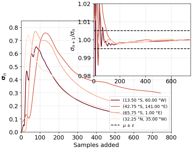
Figure 6 The convergence of the series σ_n for the temperature dataset. The outer axis shows four σ_n series, where the location of the points is given in the legend. The inner axis shows the convergence rate given in Eq. (8).

In Fig. 7a, c and e, we show the global standard deviation σ_n of S_n at the end of the month for the air temperature, wind and precipitation data, respectively. Here c=744 for the hourly temperature and wind speed data, while c=1488 for the half-hourly precipitation data. As expected, the standard deviations for all the variables are larger in areas that experience more climate variability. For example, the final standard deviation of the rolling temperature mean shown in (a) shows much larger values away from the Equator, where temperature averages will experience seasonal variation. Figure 7b, d and f show the number of samples required for the standard deviation σ_n of these rolling summaries to converge, as defined in Eq. (8), when $\left|{\mathit{\sigma }}_{n+\mathrm{1}}\right|/\left|{\mathit{\sigma }}_n\right|$ falls within the range μ±ϵ.

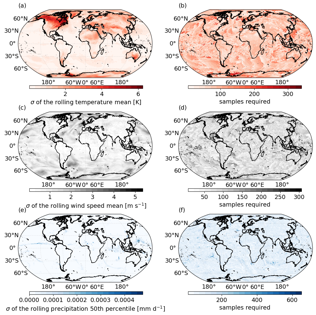
Figure 7 (a) The standard deviation of the full S_n time series at the end of the IFS monthly temperature time series during March 2020. Here $S_n={\overline{X}}_n$. (b) The number of samples required (i.e. number of time steps) for the rolling standard deviation of the S_n time series to converge. Convergence is defined in the text. (c) Same as (a) but for the IFS monthly wind speed time series in December 2020. (d) Same as (b) but for wind speed. (e) Same as (a) and (c), but here S_n is the estimate of the 50th percentile using the ICON precipitation time series in August 2021. (f) Same as (b) and (d) but for precipitation.

Encouragingly, the convergence time does not have a strong correlation with the final standard deviation σ_n shown in the left column. This is reassuring, as it shows that convergence is partially independent of the actual spread of the data and allows conservative estimates of sample size to be used for global data. What is particularly noteworthy is that, across all these datasets, the number of samples required for convergence is extremely similar. Taking the mean value of Fig. 7b, d and f results in 82, 77 and 81 samples, respectively. This is striking, especially given that Fig. 7f represents the convergence of the 50th-percentile estimate, as opposed to the mean in Fig. 7b and d. This indicates that, for hourly and half-hourly data, approximately 4 d is required to accurately represent the month. Overall, in this section we present how the one-pass algorithms provide added value in the context of bias adjustment for streamed climate data. We present criteria for stabilization that we use to define how many samples are required to be added to a rolling one-pass summary S_n before that summary can be used as a representation of the whole distribution.

8 Conclusions

Within the climate modelling community, the generation of increasingly larger datasets from kilometre-scale GCMs is becoming almost inevitable. While there is a clear argument for the added value of these high-resolution models, new challenges of handling, storing and accessing the resultant data are emerging. One novel method being investigated within the DestinE project (Bauer et al., 2021; Hoffmann et al., 2023) is data streaming, where climate variables at native model resolution are passed directly to downstream impact models in near-real model runtime. This article presents the algorithms behind the One_Pass (v0.8.0) package, designed to handle streamed climate data at the kilometre scale. The application of each algorithm has been demonstrated through relevant use cases in the context of climate change impact studies. We categorized the statistics into two different groups: a first group that can be represented by a single floating-point value and a second group which requires a distribution estimate. For the first group, which requires only a single value (e.g. mean, standard deviation, minimum, maximum, threshold exceedance), we obtain accuracy on the order of machine precision, well beyond the accuracy required or indeed provided by climate models themselves. While providing the same result as the conventional method, these algorithms allow the user to keep only a few rolling summaries in memory at any moment in time. Unlike a conventional statistic, where the memory requirements for computation scale linearly as the time series grows, the one-pass algorithms for these statistics provide an easily implemented, user-oriented method that bypasses these potentially unfeasible memory requirements.

For the statistics that require a representation of the distribution (e.g. percentiles and histograms), we applied the t-digest method, framed within relevant use cases. In Sect. 6.2 we focus on wind, a variable which requires an accurate representation of the full distribution, useful in the context of renewable energy. We recommend using a compression factor of δ=60 (approximately 80 clusters), where the mean absolute percentile differences for global monthly wind speeds did not exceed 0.9 % of the estimate given by the conventional method. For precipitation, given in Sect. 6.3, we focus on the extremes of skewed precipitation distributions. Due to the presence of low-frequency extreme events, there was more discrepancy between the NumPy and t-digest estimates. In the cases of high differences between the two estimates, there were also large error bars from the different interpolation schemes of NumPy. Examining these distributions showed that these higher differences were due to the sparseness of data in the distribution as opposed to poor representation from the t-digest. In the cases of high percentile differences, these were unrealistic differences that occurred due to division by extremely small numbers generated from the NumPy estimate and also occurred when precipitation fell around 0 to 1 mm d⁻¹, negligible values in terms of the user interested in extreme rainfall events. Overall, when averaging the differences globally, we obtained (for δ=60) 2.63 % or 0.91 mm d ⁻¹ in actual terms. We noted three methods for improving the t-digest estimate for precipitation: (a) use a different scale function (not currently implemented in the One_Pass package); (b) set a threshold for the data (i.e. ignore all samples below 1 mm d⁻¹); (c) examine the t-digest histograms rather than a single-percentile estimate. We also recommended a slightly higher compression factor of δ=80.

In Sect. 7, we present the concept of convergence for the one-pass statistical summaries S_n. While one-pass algorithms provide immediate access to evolving statistical summaries, their reliability for distribution-based applications like bias adjustment depends on the stability of the underlying estimates. Our convergence analysis offered a practical guideline for determining when these summaries can be considered representative of the full distribution. This does not imply that the climate variables themselves have stabilized but rather that the evolving summary has reached a usable approximation (i.e. a sufficiently representative estimate of the complete time series). By quantifying convergence in this way, we provide users with the tools to make informed decisions about when to trust and apply one-pass statistics in downstream statistical applications, such as quantile–quantile mapping.

Overall, we have demonstrated the effectiveness of one-pass algorithms on streamed climate data and provided their Python implementation in the One_Pass package, ready for use in data streaming workflows (Alsina-Ferrer and Grayson, 2025a). These algorithms not only provide accuracy well within the required limits of climate model variables but also empower users to harness the full potential of high-resolution data, in both space and time. Indeed, while some of the methods contain small errors (specifically the t-digest), we note that not harnessing the added value of high-resolution data due to storage limitations will also incur a potentially more significant error. Due to the fact that only a few rolling summaries are required to be kept in memory, these statistics become time-independent, allowing users dealing with high-resolution GCMs to select any variables at their native model resolution and process them in near-real model runtime. This has the potential to eliminate the constraints experienced by some users when relying on pre-defined archives of set climate variables, typically provided months to years after the simulations have been completed. With the continuing movement towards higher resolution, climate data streaming will become a fundamental paradigm of data processing and analysis. This paper showcases the features of one-pass algorithms across a range of relevant statistics that can be harnessed to work in the new era of data streaming.

Appendix A: Convergence order estimate

As both q and μ are unknown in Eq. (7) the order of convergence was estimated using

$$\begin{array}{}\text{(A1)}& q\approx {\displaystyle \frac{\log \left|\frac{{\mathit{\sigma }}_{n+\mathrm{1}}-{\mathit{\sigma }}_n}{{\mathit{\sigma }}_n-{\mathit{\sigma }}_{n-\mathrm{1}}}\right|}{\log \left|\frac{{\mathit{\sigma }}_n-{\mathit{\sigma }}_{n-\mathrm{1}}}{{\mathit{\sigma }}_{n-\mathrm{1}}-{\mathit{\sigma }}_{n-\mathrm{2}}}\right|}}.\end{array}$$

When Eq. (A1) was calculated over σ_n for a random selection of grid points, the approximation of q (for all variables) was centred around 1. This indicated a linear convergence rate for all the standard deviation time series over the global grid cells.