Numerical simulations of ocean surface waves along the Australian coast with a focus on the Great Barrier Reef

Numerical simulations of ocean surface waves along the Australian coast are performed with the spectral wave model WAVEWATCH III (WW3) and the state-of-the-art physics and numerics. A large-scale, high-resolution (1–15 km) unstructured mesh is designed for better resolving the extensive Australian coastline. Based on verification against altimeter and buoy observations, it is found that the WW3 simulations, with an observation-based source term package (i.e., ST6) and other relevant physical processes, perform reasonably well in predicting wave heights and periods in most regions. Nonetheless, the Great Barrier Reef (GBR) represents a challenging region for the wave model, in which wave heights are severely overestimated because most of the individual coral reefs and their strong dissipative effects could not be resolved by the local mesh. A two-step modeling strategy is proposed here to address this problem. First, individual coral reefs are regarded as unresolved obstacles and thus complete barriers to wave energy. Second, we adopt the unresolved obstacles source term proposed recently to parameterize the dissipative impact of these subgrid coral reefs. It is then demonstrated that this subgrid-scale reef parameterization enhances the model performance in the GBR dramatically, reducing the wave height bias from above 100 % to below 20 %. The source term balance and the sensitivity of model results to the grid resolution around the GBR are also discussed, illustrating the applicability of this two-step strategy to km-scale wave simulations.

1 Introduction

Wind-generated waves are one of the most ubiquitous phenomena in the ocean. Understanding ocean surface waves is fundamentally important for marine weather forecasts, ocean engineering design, ship navigation, coastal zone management, marine ecological protection, and ocean renewable energy assessment (e.g., Cavaleri et al., 2012; Hemer et al., 2017; Komen et al., 1994; Lowe and Falter, 2015). Ocean waves also play a vital role in modulating air–sea interactions, stirring upper ocean layers, and shaping sea ice morphology (e.g., Babanin, 2006; Belcher et al., 2012; Donelan et al., 2012; Squire, 2020). In nearshore regions, wave processes such as intensive wave breaking and wave-induced mixing are critical components for coastal modeling as well (e.g., Burchard et al., 2008; Warner et al., 2010).

Over the past two decades, the accuracy of the spectral wave modeling in global oceans has been improved significantly, owing to better physics parameterizations (particularly for wave breaking; e.g., Ardhuin et al., 2010; Babanin, 2011; Romero, 2019), the enhanced quality of wind forcing (e.g., Hersbach et al., 2020; Saha et al., 2010), and a more accurate nonlinear four-wave interaction term (e.g., Liu et al., 2019; Tolman, 2013). Liu et al. (2019) clearly demonstrated that one of the state-of-the-art source term packages, namely, the observation-based source terms ST6 available in the spectral wave model WAVEWATCH III (hereafter WW3; The WAVEWATCH III^® Development Group (WW3DG), 2019) for wind input, wave breaking, and swell decay, performs fairly well in deep waters in predicting both conventionally used wave parameters (e.g., wave height and period) and high-order spectral moments (e.g., mean square slope). Forced by the ERA5 reanalysis winds, the long-term WW3-ST6 global wave hindcast of Liu et al. (2021) shows excellent agreement with open-water altimeter wave height observations (correlation coefficient of 0.97). It was further suggested by Liu et al. (2023) that this high-quality wave hindcast could even be used as a homogeneous baseline to corroborate the relative performance of different calibration methodologies of altimeter wave records (Young and Ribal, 2022). Nonetheless, the accuracy of global wave simulations generally degrades considerably in coastal waters primarily due to coarse global bathymetric grids (usually 0.25–0.5°; see, e.g., https://confluence.ecmwf.int/display/WLW/Models, last access: 1 September 2025) and more complex physical settings (e.g., emerging bottom processes and intensive wave–tide interactions; Cavaleri et al., 2018; Moghimi et al., 2020; Tolman, 1995). Liu et al. (2021) reported that the error in wave height, H_s, from their global simulations is much larger on the Australian and Chinese coasts than that in deep oceans (scatter index of 0.2–0.4 vs. 0.15; see their Fig. 11).

This paper is dedicated to numerical simulations of ocean surface waves along the Australian coast using the wave model WW3. The purpose of this paper is 3-fold. First, as a follow-on to Liu et al. (2021), this study investigates more thoroughly the performance of the ST6 source term package, together with other relevant physical processes, in the entire Australian coastal waters. Previous applications of the WW3 and ST6 around Australia mostly focused on relatively smaller regional scales (Liu et al., 2022; Zieger et al., 2021) and shorter temporal scale (Zieger and Peach, 2023).

Second, the triangular unstructured grid technique in WW3 has evolved quickly over the past several years, and a new parallelization algorithm and an implicit time integration scheme implemented recently open up new opportunities for computationally efficient, large-scale, high-resolution unstructured modeling with WW3 in coastal and nearshore regions and even in global oceans (Abdolali et al., 2020a, b; Gaffet et al., 2025; Roland and Ardhuin, 2014). To better resolve the extensive Australian coastline, we designed a large-scale unstructured grid covering the entire Australian coastal waters, outstretching from the coastline at the highest resolution of 1 km to approximately 200–300 km offshore at the coarsest resolution of 15 km. The applicability of these newly developed unstructured schemes in WW3 is well demonstrated in our wave simulations.

Third, and the most important, during this investigation, we found that the most challenging region for our regional wave model is the Great Barrier Reef (GBR), located in the western Coral Sea off the coast of Queensland, Australia. The GBR, as the world's largest coral reef system, is composed of over 2900 individual reefs and stretches over 2300 km along the northeast shelf of Australia. Although covering a very long distance, the GBR occupies only a small fraction of the shelf area (about 9 %; 20 000 km² out of 224 000 km²; Hopley et al., 2007). The geomorphology of individual reefs may be very irregular and vary significantly from one to another, while the density of reefs changes significantly along the length of the GBR. The scattered nature of this splendid reef matrix presents very fine details to the bathymetry and poses a tremendous difficulty for wave simulations in this specific region. Previous field experiments showed that barrier reefs would induce substantial loss of incident wave energy due to the combined effect of depth-induced wave breaking and bottom friction (Hardy and Young, 1996; Lowe et al., 2005; Young, 1989). Thus, it was shown that wave energy in the GBR was seriously overestimated by spectral wave models without accounting for these dissipative effects of barrier reefs (e.g., Hardy et al., 2000; Hemer et al., 2017; Liu et al., 2021; Young and Hardy, 1993). To address this issue here, we represented individual reefs in the GBR as unresolved obstacles in our triangular mesh (i.e., small islands) by following the framework of Hardy et al. (2000). An inherent assumption of such approach is that individual reefs may be considered as total barriers to incident wave energy, which was reasonably supported by field studies (Hardy and Young, 1996; Lowe et al., 2005). In addition, we incorporated the unresolved obstacles source term (UOST; Mentaschi et al., 2015, 2018) to parameterize the energy dissipation due to these unresolved “energy barriers”. It was found that through this two-step modeling strategy, the model performance was substantially improved.

This paper is organized as follows. Section 2 presents the theoretical background for the spectral wave modeling, describes the unstructured grid we designed for the Australian coastal waters, and explains the two-step methodology we adopted to parameterize the dissipative effects of coral reefs in the GBR, particularly for the details of the UOST. Section 3 reports the altimeter and buoy data used for model verification and the winds and ocean currents adopted to force our wave simulations. Section 4 analyzes the performance of a cascade of WW3 configurations with increasing complexity, demonstrating the overall good performance of the ST6 physics in the Australian coastal waters and, more importantly, the striking benefit of the UOST approach in the GBR region. Further discussions of the source term balance at a shallow-water wave buoy in proximity of the GBR and the sensitivity of model results to the grid resolution are given in Sect. 5, followed by a brief conclusion in Sect. 6 finalizing the paper.

2 Spectral wave modeling

2.1 Radiative transfer equation

The spectral wave model WW3 solves the wave action balance equation, also known as the radiative transfer equation (RTE), to predict the amplification, dissipation, and transformation of ocean wave energy over a slowly varying medium (i.e., water depth and currents; Whitham, 1965; Holthuijsen, 2007):

$$\begin{array}{}\text{(1)}& {\displaystyle }& {\displaystyle \frac{\partial N}{\partial t}}+{\mathrm{\nabla }}_x\cdot \left(\dot{\mathit{x}}N\right)+{\displaystyle \frac{\partial }{\partial k}}\left(\dot{k}N\right)+{\displaystyle \frac{\partial }{\partial \mathit{\theta }}}\left(\dot{\mathit{\theta }}N\right)={\displaystyle \frac{S_{\mathrm{T}}}{\mathit{\sigma }}},\text{(2)}& {\displaystyle }& {\displaystyle }\dot{\mathit{x}}={\mathit{c}}_{\mathrm{g}}+\mathit{U},\text{(3)}& {\displaystyle }& {\displaystyle }\dot{k}=-{\displaystyle \frac{\partial \mathit{\sigma }}{\partial d}}{\displaystyle \frac{\partial d}{\partial s}}-\mathit{k}\cdot {\displaystyle \frac{\partial \mathit{U}}{\partial s}},\text{(4)}& {\displaystyle }& {\displaystyle }\dot{\mathit{\theta }}=-{\displaystyle \frac{\mathrm{1}}{k}}\left({\displaystyle \frac{\partial \mathit{\sigma }}{\partial d}}{\displaystyle \frac{\partial d}{\partial m}}+\mathit{k}\cdot {\displaystyle \frac{\partial \mathit{U}}{\partial m}}\right),\end{array}$$

where $N(k,\mathit{\theta };\mathit{x},t)=F(k,\mathit{\theta };\mathit{x},t)/\mathit{\sigma }$ is the wave action density spectrum, $F(k,\mathit{\theta };\mathit{x},t)$ is the wavenumber-direction energy density spectrum, and σ is the intrinsic (radian) frequency. The terms in the LHS of Eq. (1) signify the kinematic change of wave energy, where $\dot{\mathit{x}}$ is the absolute traveling speed of wave energy and c_g is the intrinsic group velocity. Equation (3) gives the rate of change of the wave number k owing to water depth d and current velocity U varying along the wave orthogonal S. The variation in wave direction θ due to depth- and current-induced refraction is then given by Eq. (4), where m is a coordinate along the wave crest and thus perpendicular to the coordinate S. The radian frequency σ, wave number k, and group velocity c_g are determined through the dispersion relationship of the linear wave theory:

$$\begin{array}{}\text{(5)}& {\mathit{\sigma }}^{\mathrm{2}}=gk\tanh \left(kd\right),\end{array}$$

in which g is the gravitational acceleration.

The RHS of the RTE presents various physical processes modifying wave energy (i.e., sources and sinks), and in our paper, the source terms considered include:

$$\begin{array}{}\text{(6)}& S_{\mathrm{T}}=S_{\mathrm{in}}+S_{\mathrm{ds}}+S_{\mathrm{swl}}+S_{\mathrm{nl}}+S_{\mathrm{bf}}+S_{\mathrm{db}}+S_{\mathrm{uo}},\end{array}$$

in which S_in represents the atmospheric input from the wind, S_ds is the “white-capping” dissipation, S_swl is the swell decay term, S_nl is the nonlinear four-wave interactions between spectral components, S_bf is the bottom friction, S_db refers to the depth-induced breaking, and S_uo denotes the subgrid-scale parameterization of energy dissipation due to unresolved obstacles. In our simulations, we calculated $S_{\mathrm{in}}+S_{\mathrm{ds}}+S_{\mathrm{swl}}$ according to the observation-based source term package ST6 (Liu et al., 2019; Rogers et al., 2012; Zieger et al., 2015) and the S_nl term based on the discrete interaction approximation (DIA) of Hasselmann et al. (1985). The formulations for these terms are not reproduced here for brevity.

The bottom friction S_bf was due to the simple, linear JONSWAP parameterization (Hasselmann et al., 1973):

$$\begin{array}{}\text{(7)}& S_{\mathrm{bf}}(k,\mathit{\theta })=-{\displaystyle \frac{\mathrm{\Gamma }}{g^{\mathrm{2}}}}{\displaystyle \frac{{\mathit{\sigma }}^{\mathrm{2}}}{{\sinh }^{\mathrm{2}}\left(kd\right)}}F(k,\mathit{\theta }),\end{array}$$

where Γ=C_bgU_rms, C_b is the bottom drag coefficient, and U_rms is the root-mean-square bottom orbital velocity (Holthuijsen, 2007). Following Zijlema et al. (2012), a unified Γ of 0.038 m² s⁻³ was used for both wind sea and swell.

The depth-induced wave breaking S_db we adopted conforms to the semi-empirical model of Battjes and Janssen (1978), which reads as follows:

$$\begin{array}{}\text{(8)}& S_{\mathrm{db}}(k,\mathit{\theta })=-\mathrm{0.25}{Q}_{\mathrm{b}}\stackrel{\mathrm{‾}}{f}{\displaystyle \frac{H_{\max }^{\mathrm{2}}}{m_{\mathrm{0}}}}F(k,\mathit{\theta }),\end{array}$$

where $\stackrel{\mathrm{‾}}{f}=m_{\mathrm{1}}/m_{\mathrm{0}}$ is the mean wave frequency, $m_n=\underset{f}{\overset{n}{\int }}E\left(f\right)df$ is the nth order spectral moment, and Q_b is the fraction of breaking waves in the random wave field, i.e., the probability that the individual wave height is above the limiting wave height H_max in finite-depth water:

$$\begin{array}{}\text{(9)}& H_{\max }=\mathit{\gamma }d\end{array}$$

where the breaking index γ=0.73 was used in our simulations. Based on the assumption of the Rayleigh-type wave height distribution truncated at H_max, the fraction of breakers Q_b is then determined iteratively from

$$\begin{array}{}\text{(10)}& {\displaystyle \frac{\mathrm{1}-Q_{\mathrm{b}}}{\ln Q_{\mathrm{b}}}}=-{\left({\displaystyle \frac{H_{\mathrm{rms}}}{H_{\max }}}\right)}^{\mathrm{2}},\end{array}$$

in which $H_{\mathrm{rms}}=\mathrm{2}\sqrt{\mathrm{2}{m}_{\mathrm{0}}}$ is the root-mean-square wave height.

Because some details of the subgrid-scale parameterization S_uo vary with the mesh used, we will first introduce our triangular mesh in Sect. 2.2 and then present the description of S_uo in Sect. 2.3.

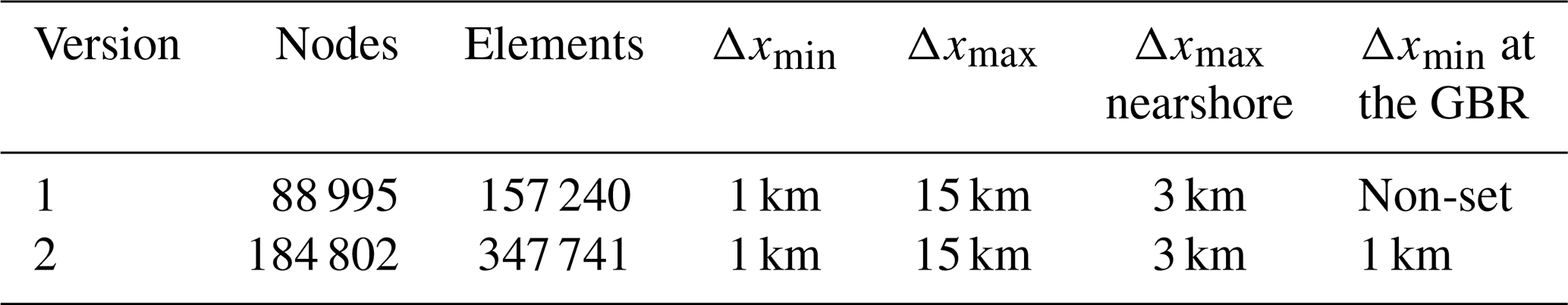
Table 1 Summary of the unstructured grids used in the WW3 simulations for 2011 discussed in the paper. Δx represents the mesh resolution.

2.2 Unstructured grid and numerics

In this study, the wave modeling along the Australian coast was performed on a high-resolution unstructured grid, stretching from the Australian coastline towards 200–300 km offshore. The spatial extent, bathymetry, and resolution of the triangular mesh are illustrated in Fig. 1. The model domain was designed in such a way that the propagation and transformation of deep-water waves into the Australian nearshore regions could be correctly captured. The water depths in the outermost part of the mesh are more than 500 m except for the Gulf of Carpentaria, the sea off the northern coast of Australia, in which the water depth is generally below 70 m (Fig. 1a). We generated the triangular mesh with the OceanMesh2D toolkit (Roberts et al., 2019) using the SRTM15+ bathymetric dataset (15 arcsec; Tozer et al., 2019), with the highest resolution of 1 km along the shoreline boundary and the coarsest resolution of 15 km near the open boundaries. A smooth transition of the mesh resolution from the coastline to open oceans is assured through using the “feature” mesh size function of OceanMesh2D (Roberts et al., 2019), which distributes the mesh resolution in the model domain according to the geometric width of the coastline (Fig. 1c; more curved coastlines correspond to smaller geometric widths and smaller feature size and thus to higher grid resolutions). We further constrained the nearshore triangular element size (within 0.1° of the coastline) to not exceed 3 km (Fig. 1b). The resultant unstructured grid consists of a total of 88 995 nodes and 157 240 elements (mesh Version 1 in Table 1).

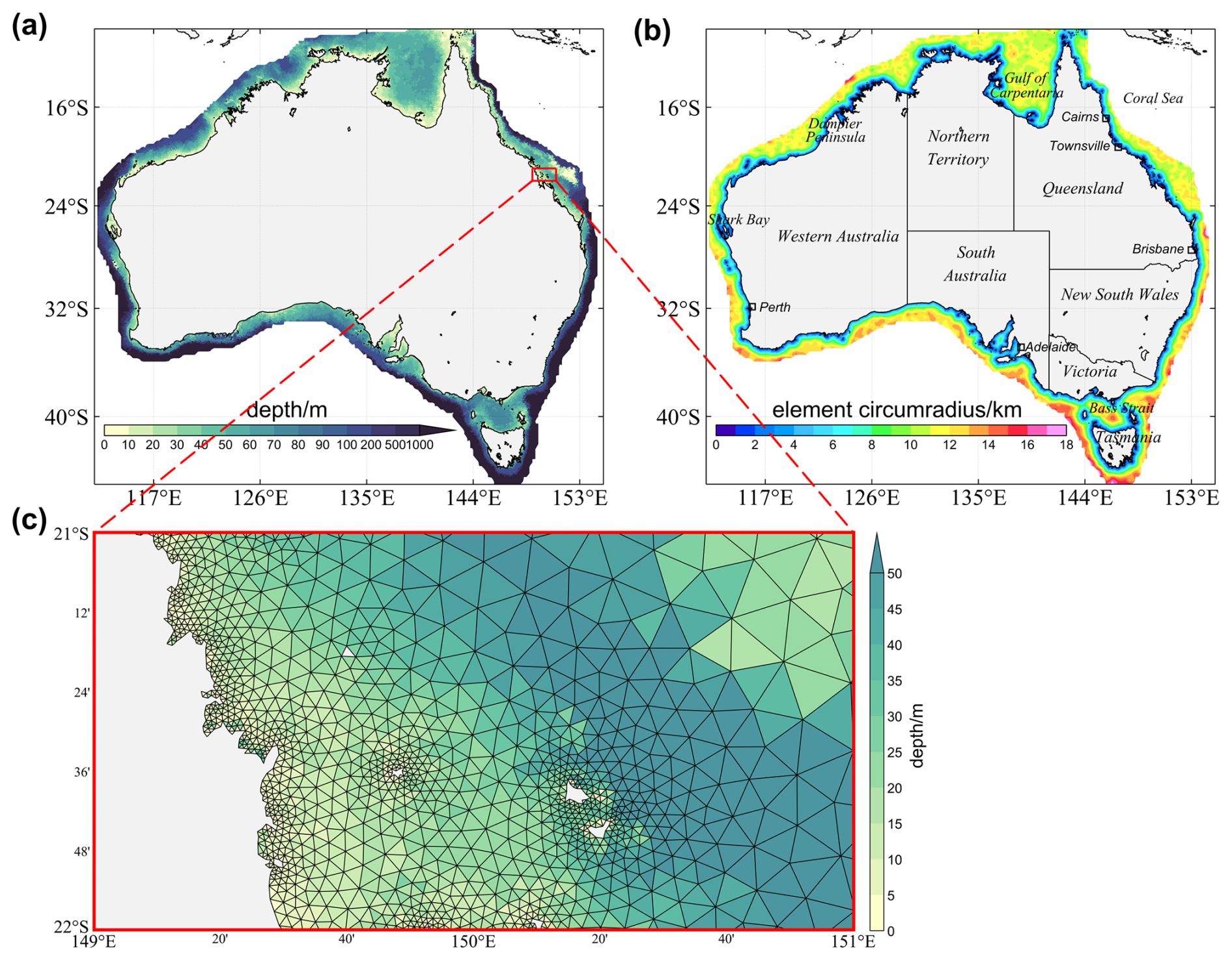
Figure 1 The (a) bathymetry (in meters) and (b) mesh resolution (in terms of the local element circumradius; unit: km) of the high-resolution triangular mesh along the Australian coast. (c) A triangular grid with varying resolutions presenting an enlarged view of a 1°×2° bin off the northeast coast of Australia.

The geographical space derivative of the wave spectrum on the triangular mesh was based on the contour residual distribution (Roland, 2009), and we performed the time integration using an implicit first-order upwind scheme (Abdolali et al., 2020b) with a global time step of 1200 s. The domain decomposition parallelization method was adopted to improve the scalability and efficiency of our simulations. The spectral grid is logarithmically spaced over 35 frequencies, ranging from 0.037 to 0.953 Hz with an increment factor of 1.1, and the directional grid is equally spaced with an interval of 10°. In addition, the two-dimensional wave spectra F(f, θ) along open boundaries were sourced from the WW3-ST6 global wave hindcast of Liu et al. (2021).

2.3 Wave attenuation over coral reefs

As mentioned in the Introduction, owing to its magnificent extent and remarkable porosity (i.e., significant inner-reef gaps), the GBR stands as the most demanding region for our simulations (Fig. 2). The wave age ($c_{\mathrm{p}}/U_{\mathrm{10}}\mathrm{\Delta }\mathit{\theta }$, where c_p is the phase velocity for the peak wave frequency, U₁₀ is the 10 m wind speed, and Δθ denotes the angle between the wind direction and peak wave direction) distribution (Fig. 2c) indicates that the seaward side of the GBR is primarily dominated by swell from the Coral Sea (Smith et al., 2023). Over the reef matrix, the wave field is largely composed of wind sea, characterized by relatively low wave age values (0.5–1), whereas the inter-reef gaps remain significantly influenced by offshore swell. In the lee of the reef, locally generated waves become the dominant component of the wave field (Gallop et al., 2014). This pattern suggests that the coral reefs effectively dissipate long-period wave energy. Field experiments clearly confirmed that coral reefs are natural wave energy sinks (Hardy and Young, 1996; Lowe et al., 2005). The presence of a coral reef typically will introduce abrupt changes in water depth, thus forming a steep reef front, followed by a remarkably shallow, flat reef crest with a depth of a few meters (Zieger et al., 2009). Over the leeward side of the reef, a relatively deep lagoon may appear (see, e.g., Fig. 1 of Lowe et al., 2005). The sloping fore reef generally results in a substantial loss of incident wave energy because of the depth-induced wave breaking and bottom friction occurring at the seaward edge of the reef. As waves propagate onto the even shallower reef crest, wave energy will be further dissipated by the bottom friction. Wave heights on reef crests were found to be strongly modulated by the tidal elevation (and thus local water depth; see, e.g., Fig. 5 of Hardy and Young, 1996).

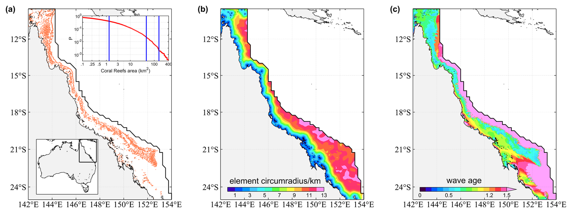
Figure 2 (a) The northeastern coast of Australia and the Great Barrier Reef (GBR; orange color) located inside our model domain (delimited by the black curve). The reef outlines (polygons) are from the multi-source global dataset of warm-water coral reefs compiled by UNEP-WCMC et al. (2010; version 4.1 with the highest resolution of 30 m). The inset displays the exceedance probability distribution of the area of individual reef polygons. The three blue vertical lines highlight the areas for characteristic equilateral triangular elements with a circumradius of 1, 6, and 11 km, respectively. (b) Same as Fig. 1b but for the mesh resolution zoomed in around the GBR. (c) Spatial distribution of wave age in the GBR based on the Run 7 simulation (see Table 2) for the year 2011.

The challenges for simulating waves in the GBR include the following two aspects. First, individual reefs in this complex reef matrix are generally small in terms of their spatial scales and thus could not be resolved by the triangular mesh we designed. Figure 2 suggests (i) that only 2 % of reef polygons could be resolved by a triangular element with a 6 km circumradius, the average mesh resolution around the GBR, and (ii) that even the finest 1 km element will fail to capture approximately 60 % of reef polygons. Both the formulations of the bottom friction S_bf (Eq. 7) and depth-induced breaking S_db (Eq. 8) require information on the local water depth. Missing individual reefs in the bathymetric grid would apparently lead to underestimation of the dissipation arisen from these two processes. Second, even if these small individual reefs are resolved properly, tremendous difficulties remain to establish reasonable physics parameterizations of S_bf and S_db to model spectral transformation over coral reefs. The formulation of S_db due to Battjes and Janssen (1978) was derived for relatively mild bottom slopes and may not be applicable to coral reefs with very steep slopes (Massel and Gourlay, 2000). Because of the presence of reef organisms, coral reef surfaces could be 2–3 orders of magnitude rougher than sandy beaches, closely depending on the canopy structure of reefs (Lowe et al., 2005; Monismith et al., 2015). Nonetheless, it is extremely difficult, if not impossible, to survey the bottom roughness of all the individual reefs of the GBR, and obviously, the JONSWAP friction with a constant Γ found from sandy bottoms (7) is bound to fail to efficiently dissipate wave energy over these rough coral reefs.

To circumvent these difficulties, two different strategies have been suggested by previous studies on wave simulations in the GBR:

1. A hierarchy of nested grids was created so that the mesh resolution around specific coral reefs is locally enhanced and thus better resolved. These resolved reefs are then represented by land (Young and Hardy, 1993) or submerged islands (Zieger and Peach, 2023).

2. The dissipation of wave energy induced by coral reefs is considered as a subgrid-scale process and then is implemented within the numerical advection scheme. Wave energy fluxes are partially reduced when flowing though grid cells containing “subgrid” reefs (Hardy et al., 2000).

Both of these methods assume that coral reefs represent almost complete wave energy barriers, which are well supported by field observations (Hardy and Young, 1996; Lowe et al., 2005; Young, 1989), at least for long-period swells. Following these pioneering studies, we treated individual reefs in the GBR as unresolved islands in the median dual cells associated with the mesh nodes. Different from Hardy et al. (2000), this subgrid dissipative process was characterized by a source-term-based approach rather than the propagation-based numerical approach. Specifically, we used the UOST parameterization formulated by Mentaschi et al. (2015, 2018) to quantify the dissipative effect of the unresolved reefs (islands). For each median dual cell:

$$\begin{array}{}\text{(11)}& {\displaystyle }{S}_{\mathrm{uo}}=S_{\mathrm{ld}}+S_{\mathrm{se}},\text{(12)}& {\displaystyle }{S}_{\mathrm{ld}}=-{\mathit{\psi }}_{\mathrm{ld}}{\displaystyle \frac{\mathrm{1}-{\mathit{\beta }}_l}{{\mathit{\beta }}_l}}{\displaystyle \frac{c_{\mathrm{g}}}{\mathrm{\Delta }L}}F(k,\mathit{\theta }),\text{(13)}& {\displaystyle }{S}_{\mathrm{se}}=-{\mathit{\psi }}_{\mathrm{se}}\left({\displaystyle \frac{{\mathit{\beta }}_u}{{\mathit{\alpha }}_u}}-\mathrm{1}\right){\displaystyle \frac{c_{\mathrm{g}}}{\mathrm{\Delta }L}}F(k,\mathit{\theta }),\end{array}$$

where S_ld represents the dissipative effect of unresolved obstacles on the cell-averaged wave energy, namely, the local dissipation, S_se represents the correction (reduction) of ingoing wave energy owing to the presence of unresolved obstacles in its upstream cells, namely, the shadow effect, and ΔL is the path length of a given spectral component k in the cell and varies with the wave direction θ. The ψ_ld and ψ_se factors represent the empirical reduction of the dissipation in the presence of local wave growth, depending on the wave age $\mathit{\delta }=\frac{c}{U_{\mathrm{10}}\cos (\mathit{\theta }-{\mathit{\theta }}_u)}$ in the following form (The WAVEWATCH III^® Development Group (WW3DG), 2019):

$$\begin{array}{}\text{(14)}& {\mathit{\psi }}_{\mathrm{ld}}={\mathit{\psi }}_{\mathrm{se}}=\left\{\begin{array}{ll}\mathrm{0},& \mathrm{for}\mathit{\delta }\le \mathrm{0.5}\\ \frac{\mathit{\delta }-\mathrm{0.5}}{\mathrm{1.5}-\mathrm{0.5}},& \mathrm{for}\mathrm{0.5}<\mathit{\delta }<\mathrm{1.5}\\ \mathrm{1},& \mathrm{for}\mathit{\delta }\ge \mathrm{1.5}\end{array}\right.,\end{array}$$

in which U₁₀ and θ_u denote the 10 m wind speed and direction, respectively.

The blocking effect of subgrid obstacles is characterized by two transparency coefficients, α and β. The total transparency coefficient α depends on the cross section δ of unresolved obstacles in the cell along the wave propagation direction (Mentaschi et al., 2018):

$$\begin{array}{}\text{(15)}& \mathit{\alpha }(\mathit{x},\mathit{\theta })=\mathrm{1}-\mathit{\delta }(\mathit{x},\mathit{\theta }).\end{array}$$

α=0 corresponds to a fully blocked cell, and α=1 corresponds to an obstacle-free cell. The layout-dependent transparency β accounts for the distribution of the obstacles inside the cell and is defined as the average transparency of cell subsections starting from the upstream side of the cell (Fig. 3). If the obstacles are near the cell upstream side, β will be quite close to α; if the obstacles, however, are in proximity to the cell downstream side, β∼1. In any event, α≤β. In Eqs. (12) and (13), the subscripts “l” and “u” for α and β denote that these coefficients are defined for the local cell and its upstream polygon, respectively. Figure 3 illustrates how α and β are estimated for a given median dual cell and its upstream polygon for the wave direction specified. The reader is referred to Mentaschi et al. (2015, 2018, 2019) for more technical details of the UOST approach.

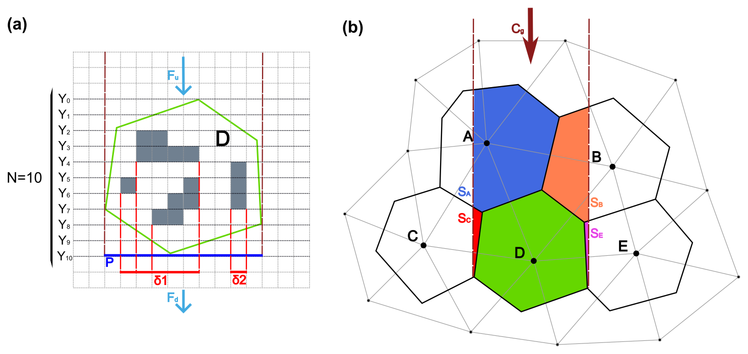
Figure 3 (a) Calculation of the local transparency coefficients α_l and β_l in a median dual cell D (green hexagon). F_u and F_d are the ingoing and outgoing spectral energy density, respectively. Here, the cell is horizontally sub-divided into 10 slices. The gray squares represent unresolved obstacles, and the red dotted lines highlight squares sheltered by these unresolved obstacles. The projection of the cell D along the wave direction is represented by the blue line segment P, and the projections of the obstacles are shown as δ₁ and δ₂. In this case, the total transparency ${\mathit{\alpha }}_l=(P-{\mathit{\delta }}_{\mathrm{1}}-{\mathit{\delta }}_{\mathrm{2}})/P=\mathrm{0.4}$. The layout-dependent transparency β_l is defined as the average of α_l,i for each successive subsection starting from the upstream side of the cell (i.e., α_l,1 corresponds to the subsection Y0–Y1, α_l,2 to Y0–Y2, etc.); here, β_l=0.59. (b) The cell D (green hexagon) and its upstream polygon for the wave direction shown by the brown arrow. The upstream polygon consists of the portions of upstream cells swept by the wave energy flux towards the cell D (S_A, blue; S_B, orange; S_C, red; S_E, purple). Thus, the total area covered by the upstream polygon is $S=S_A+S_B+S_C+S_E$, ${\mathit{\alpha }}_u=({\mathit{\alpha }}_{l,A}{S}_A+{\mathit{\alpha }}_{l,B}{S}_B+{\mathit{\alpha }}_{l,C}{S}_C+{\mathit{\alpha }}_{l,E}{S}_E)/S$, and β_u is calculated in the same way.

Estimation of these transparency coefficients for our unstructured mesh was achieved through the open-source package alphaBetaLab (https://github.com/menta78/alphaBetaLab, last access: 1 September 2025) developed by Mentaschi et al. (2019). Apart from the unstructured mesh, alphaBetaLab requires a bathymetric dataset at a much higher resolution than the mesh itself. We adopted the SRTM15+ bathymetry for this purpose. We further extracted the reef outlines of the GBR (Fig. 2) from the multi-source global coral reef dataset complicated by UNEP-WCMC et al. (2010; highest resolution of 30 m), and any sea points of the SRTM15+ located within these reef outlines were transformed into land points. Figure 4 illustrates the transparency coefficients α and β for parts of the GBR regions. There are too many fine details to be explained in these plots. Nonetheless, it is observed that the scattered individual reefs are effectively represented by these directional transparency coefficients, with cells in close proximity to reefs having α and β values remarkably lower than 1 (Fig. 4b and d). More importantly, for most of the cells shown, the total transparency α in the directions perpendicular to the orientation of the reefs is clearly lower than that parallel to the reef orientation. It is also noteworthy that the local transparency α_l conforms to a 2-fold rotational symmetry (e.g., α_l(0°)=α_l(180°); Fig. 4b), as expected from its definition (Eq. 15). On the contrary, the upstream overall transparency α_u is asymmetric owing to changes in the extent of the upstream polygons with the wave propagation direction (Fig. 4d).

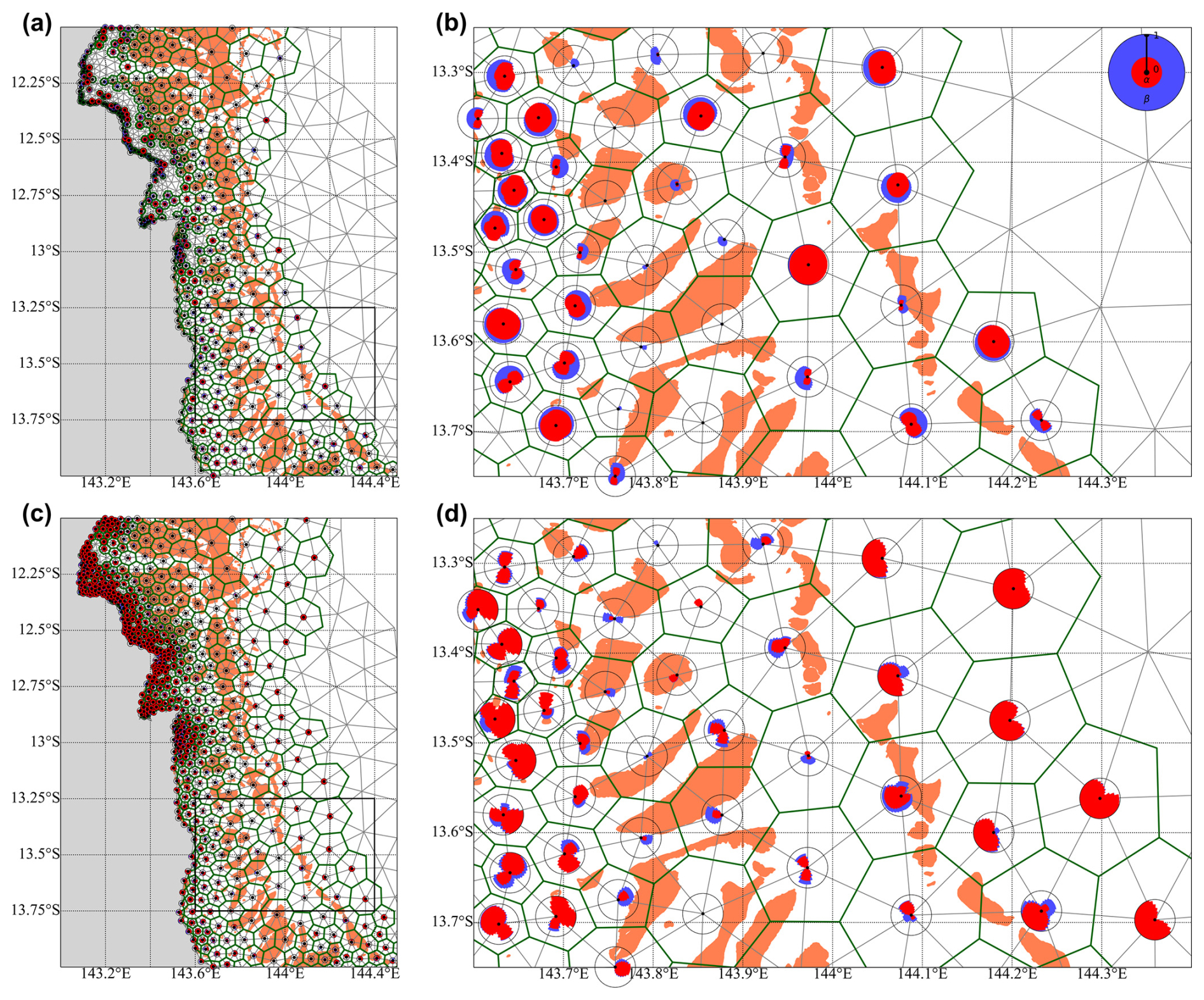
Figure 4 Illustration of the directional transparency coefficients α (red pie) and β (blue pie) for (a, b) the local dissipation α_l, β_l and for (c, d) the shadow effect α_u, β_u, respectively, in parts of the GBR. (b, d) A zoomed-in view of the region outlined by the black box in (a, c). The thin gray lines denote the triangular elements, and the green lines are the median dual cells connecting the centroids of the triangles. Both α and β are evaluated at the mesh nodes. Individual reef polygons are shown with orange shading. A full pie indicates a transparency of 1 for all the directions, whereas an incomplete pie suggests that wave energy in specific directions will be dissipated due to the presence of reefs inside a given cell or its upstream polygon. Here, θ in the pie plots denotes the wave propagation direction, taken counterclockwise from the geographic east (i.e., waves propagating eastward and northward have θ=0° and θ=90°, respectively).

Figure 5, from a different point of view, shows the spatial distribution of these transparency coefficients in the GBR, in which the minimum and maximum α(θ) and β(θ) and the directions for these minima and maxima are presented. Because the GBR mainly stretches along the direction NW–SE south of 15° S and along the direction N–S equatorward of 15° S, the minimum α_l and β_l are frequently located in the NE–SW and E–W octants (waves in these directions will be the most heavily dissipated). On the other hand, it is not uncommon to observe the maximum α_l and β_l located in N–S and NW–SE octants, parallel to the elongated layout of the GBR. A remarkable result is that the spatial extent of low α_u and β_u values for the shadow effect (e.g., α_uβ_u≤0.2) is considerably larger than that of low α_l and β_l values for the local dissipation (Fig. 5a and c vs. Fig. 5e and g), demonstrating the relatively far-reaching effect of these reefs. Through altimeter wave data, Young (1989) also reported that isolated reefs induced a significant reduction in wave energy many kilometers away from these reefs.

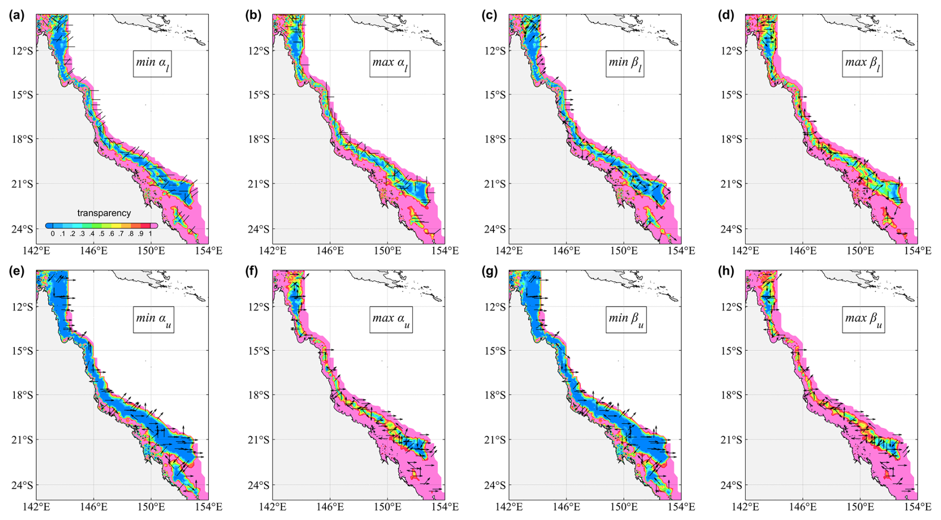
Figure 5 Spatial distribution of transparency coefficients α and β in the GBR: (a) min{α_l(θ)}, (b) max{α_l(θ)}, (c) min{β_l(θ)}, and (d) max{β_l(θ)}. (e–h) Same as (a)–(d) but for α_u and β_u. The arrows denote the directions to which these maxima and minima correspond. The head of the arrows is not shown in (a, b) because of the symmetry of α_l. For visual clarity, only arrows at nodes with a circumradius larger than 6 km were drawn, and the density of arrows were further reduced by a factor of 5 and 8 for the local and upstream coefficients, respectively.

3 Observations and model forcings

3.1 Altimeter data

In this study, we used the altimeter data (significant wave height H_s and wind speed U₁₀) of Ribal and Young (2019) and Young and Ribal (2022) to evaluate wind forcings and validate our WW3 simulations. For the year 2011 we considered, four altimeters (i.e., ENVISAT, JASON-1, JASON-2, and CryoSat-2) were flying in orbit and thus were selected for the following verification. Altimeter records less than 50 km offshore were excluded from our analysis to avoid land contamination.

When compared against satellite observations, the equally spaced wind forcing was interpolated bilinearly in space and linearly in time to the altimeter spatiotemporal locations, whereas the WW3 outputs on the unstructured grid were interpolated in space using the nearest neighbor interpolation. Following Liu et al. (2021), these model–altimeter 1 Hz matchups were further aggregated into 1°×1° bins, and for a given altimeter pass transversing a specific 1°×1° bin, the along-track averaging was performed to obtain a statistically stable model–altimeter collocation. Error metrics used in this study include the bias (b), RMSE (ε), correlation coefficient (ρ), scatter index (SI), and normalized bias (b_n) and RMSE (ε_n), for which the definitions can be found, for example, in Liu et al. (2016, 2019). Thus, the formulae for these metrics are not reproduced here for brevity.

3.2 Buoy data

The wave buoy observations used in this study were obtained from the Australian Ocean Data Network (AODN). A total of 28 wave buoys were maintained by the Australian Bureau of Meteorology (BoM), the Queensland Department of Environment and Science (DES), the Western Australia Department of Transport (DOT), and the Integrated Marine Observing System (IMOS) in 2011. Figure 6 presents the specific locations and water depth of the 28 buoys selected. More details of these buoys are provided in the supporting online material (Sect. S5). Three wave parameters (significant wave height, H_s; mean zero-crossing period, T₀₂; and peak wave period, T_p) from these buoys were used for model validations. It might be noteworthy, however, that T₀₂ is not available at the coastal buoys of Western Australia. Outliers in wave observations were excluded through a quality control procedure by following Caires and Sterl (2003) and Liu et al. (2016).

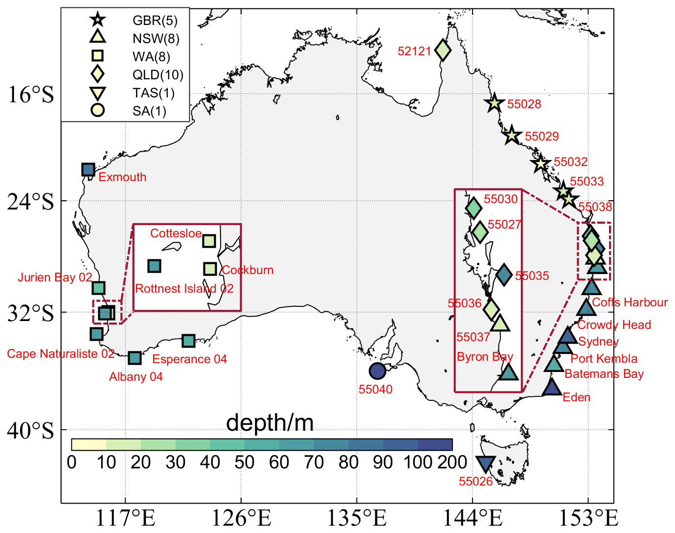
Figure 6 Locations and water depth of wave buoys sourced from the AODN used for validating wave simulations. For clarity, zoomed-in views of the wave buoys near Perth and Brisbane are shown in the left and right insets, respectively. Buoys are grouped according to the Australian administrative divisions, including New South Wales (NSW), Western Australia (WA), Queensland (QLD), Tasmania (TAS), and South Australia (SA). Note that the wave buoys in the GBR, although belonging to the QLD group, are highlighted separately with star symbols.

3.3 Wind forcing

The accuracy of the wind forcing is generally one of the most important factors defining the performance of spectral wave models, particularly for deep-water simulations (e.g., Janssen, 2008). For our coastal simulations, we experimented with wind data sourced from three different reanalysis datasets, namely, the ERA5 (hourly, 0.25°×0.25°; Hersbach et al., 2020), CFSv2 (hourly, 0.205°×0.205°; Saha et al., 2010, 2014), and Bureau of Meteorology atmospheric high-resolution regional reanalysis for Australia (BARRA; hourly, 0.11°×0.11°; Su et al., 2019) (Fig. S1 in the Supplement). The first two wind datasets are widely used globally (e.g., Ardhuin et al., 2010; Chawla et al., 2013; Liu et al., 2021), and the BARRA dataset covers the entirety of Australia at a much higher spatial resolution than the former two.

Table 2 Summary of the WW3 simulations for 2011 discussed in the paper, with different forcings and settings.

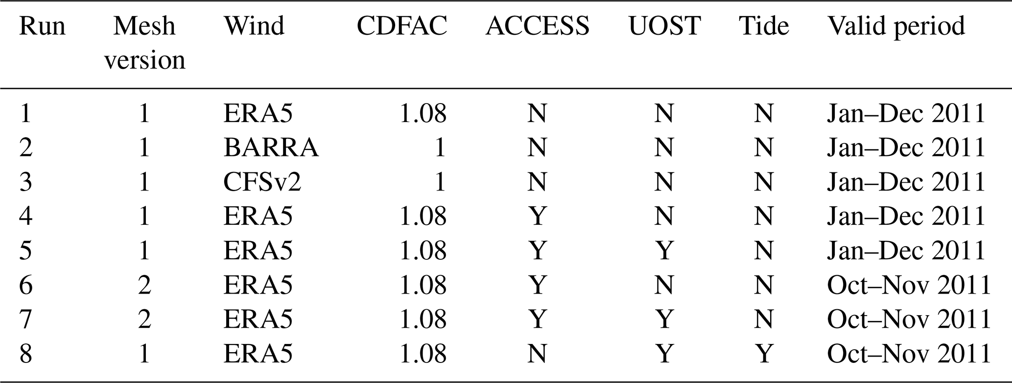
Note: here, CDFAC is the tunable wind stress parameter of the ST6 source term package. “Tide” includes tidal elevation and tidal currents. The symbol “Y” and “N” denote whether the respective setting is used or not.

We intercompared these three wind datasets against altimeter wind observations and then investigated the sensitivity of the WW3 simulations to different wind forcings (Runs 1–3 in Table 2; see Sects. S1 and S2 in the Supplement). It was found that our simulations were relatively insensitive to the wind forcings used because of the relatively limited extent of our wave model domain (Fig. 1). Nonetheless, considering that the ERA5-forced run performs marginally better than the other two (Fig. S2), and for consistency with the open-boundary wave spectra that were produced by an ERA5-forced global WW3 simulation (Liu et al., 2021), we will adopt ERA5 as the wind forcing for all the following runs.

3.4 Ocean surface currents

It has long been known that ocean surface currents play a remarkable role in modulating the propagation and transformation of wave energy (Peregrine, 1976; Romero et al., 2017; van der Westhuysen, 2017). Numerical studies have shown that the introduction of currents can reduce simulation errors for both the deep-water and coastal wave modeling (e.g., Rapizo et al., 2015, 2017). Thus, when necessary, we also included the ocean surface currents (daily, 0.1°) produced by the ocean–sea ice model ACCESS-OM2 (hereafter ACCESS; Kiss et al., 2020) in our wave simulations. However, it was seen that these daily surface currents resulted only in very minor changes in the overall model accuracy (Run 4 vs. Run 1 in Table 2; Sect. S3). In this regard, we note that the tidal currents were not included in the ACCESS data. Further analysis of the impact of the tidal elevation and tidal currents on our wave simulations based on the FES2014 dataset (Lyard et al., 2006, 2021) is presented in the Appendix.

4 Results

In this section, based on comparisons against altimeter observations, we will first carefully analyze the performance of our wave simulations and particularly the impact of the reef parameterization S_uo in the GBR region (Sect. 4.1 and 4.2). Verification of our simulations against wave buoy data will be subsequently given in Sect. 4.3. All the simulations presented in this section are summarized in Table 2.

4.1 Performance of wave simulations without S_uo

The spatial distribution of the H_s errors from the WW3 run forced by the ERA5 winds and ACCESS currents (i.e., Run 4 in Table 2) is presented in Fig. 7a and b. The subgrid-scale parameterization S_uo was not taken into account in this specific run. Except for the GBR, the model performs reasonably well, with the normalized bias b_n mostly ranging from −10 % to 10 % (Fig. 7a). Wave heights off the Southern Australian coast are generally overestimated by up to 10 %. More marked overestimation of H_s (10 %–20 %) is seen in the Bass Strait (between Victoria and Tasmania), the Spencer and St Vincent gulfs in the vicinity of Adelaide, and the coastal waters near Perth. On the contrary, wave heights in the northwest shelf region, near Northern Australia and offshore the state of New South Wales, are underestimated by approximately 10 %. The normalized RMSE is below 20 % for most regions in the model domain (Fig. 7b), and the Gulf of Carpentaria shows a moderately larger ε_n around 25 %. The spatial pattern of the model errors shown here is in good agreement with that of the global simulation conducted by Liu et al. (2021; their Fig. 8a), once again reflecting the dominant role of the open-boundary wave spectra in our regional and coastal simulations.

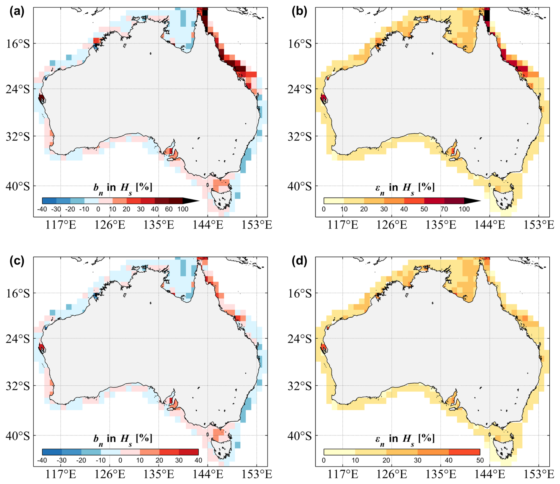
Figure 7 Error statistics of the significant wave height H_s gridded in 1°×1° bins for the WW3 (a, b) Run 4 (without the S_uo approach) and (c, d) Run 5 (with S_uo) relative to the altimeter wave records: (a, c) the normalized bias b_n and (b, d) the normalized RMSE ε_n. The ERA5 winds and ACCESS currents were adopted to force these two runs. A similar figure for the absolute bias b and RMSE ε can be found in Fig. S6.

As mentioned earlier, only very few percent of individual reefs of the GBR could be resolved by our unstructured mesh (Fig. 2a). Thus, when the dissipative effects of the GBR are totally neglected (e.g., Run 4), the local wave heights are seriously overestimated, with b_n generally larger than 40 % and up to 160 %. The regions where H_s is the most severely overpredicted are north of Cairns and in proximity to Townsville, corresponding to the areas in which the density of reefs is the highest (see also Fig. 8). The RMSE in the GBR is also strikingly high, with ε_n by and large above 50 %, and the maximum ε_n of 150 % is seen near the northernmost part of Queensland.

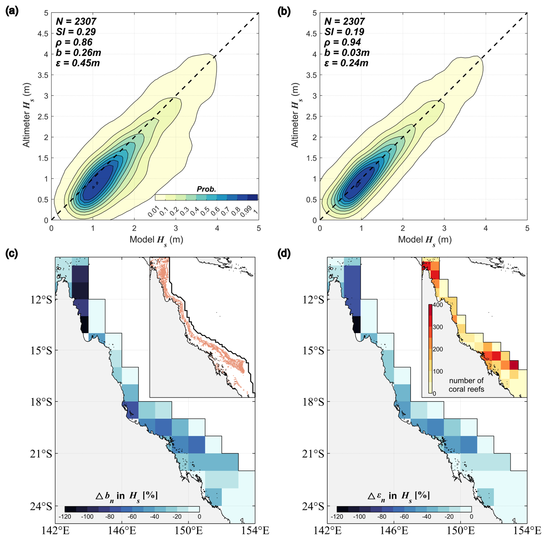
Figure 8 (a, b) Comparison of the significant wave height H_s between altimeters and WW3 simulations in the GBR region only: (a) Run 4 without S_uo and (b) Run 5 with S_uo. The error statistics of H_s for the entire model domain can be found in Fig. S5. (c, d) Differences in H_s errors between the two WW3 runs: (c) $\mathrm{\Delta }{b}_{\mathrm{n}}=b_{\mathrm{n},\mathrm{5}}-b_{\mathrm{n},\mathrm{4}}$ and (d) $\mathrm{\Delta }{\mathit{\epsilon }}_{\mathrm{n}}={\mathit{\epsilon }}_{\mathrm{n},\mathrm{5}}-{\mathit{\epsilon }}_{\mathrm{n},\mathrm{4}}$. The insets in (c, d) display the geographical locations of the GBR and the density (in terms of number) of individual reef outlines in each 1°×1° bin, respectively.

4.2 Impact of the subgrid-scale reef parameterization

In Sect. 2.3, we explained that, to enhance the model accuracy in the GBR, we adopted a two-step modeling methodology, namely, the “reef as land” and UOST approach. Here, we will show that with this subgrid-scale parameterization, the overall model performance in the GBR indeed can be improved substantially.

The H_s errors from Run 5, in which S_uo was activated (Table 2), are presented in Fig. 7c and d. Relative to the simulation without the reef parameterization (i.e., Run 4), Run 5 yields obviously much higher skills in simulating wave heights in the GBR. It is seen that the b_n in the GBR is dramatically reduced, commonly below 20 %, and ε_n is mostly lower than 30 % (Fig. 7c and d vs. Fig. 7a and b). We calculated the transparency coefficients α and β for the whole model mesh with the alphaBetaLab package (Mentaschi et al., 2019). Thus, the blocking effect of unresolved islands beyond the GBR region was also included through the UOST approach. This explains why the H_s errors in Spencer Gulf, Shark Bay, and north of the Dampier Peninsula decrease considerably as well.

Figure 8 illustrates more directly the impact of the reef parameterization S_uo on the simulated wave heights in the GBR region only. Relative to altimeter observations, the WW3 run without S_uo overestimates H_s in the GBR by 0.3 m, whereas the inclusion of S_uo leads to almost unbiased H_s and reduces the overall RMSE by 47 % (from 0.45 to 0.24 m) and SI by 1/3 (from 0.3 to 0.2; Fig. 8a and b). For regions with highly dense individual reefs, such as seas offshore the northernmost tip of Queensland, the reduction in b_n and ε_n is more than 100 % (Fig. 8c and d).

4.3 Validation against wave buoy observations

To this point, we have compared the model results only against altimeter observations, providing a macroscopic view of the model performance in simulating wave height H_s. In this section, we will present further validation of both the simulated wave height H_s and periods (T₀₂, T_p) against wave buoy measurements, adding more thorough proofs to demonstrate the skills of the reef parameterization and our wave model framework in general.

It is seen in Fig. 9 that wave heights from the full simulation (i.e., Run 5 with S_uo) are in excellent agreement with the buoy observations, with a bias less than 0.1 m and correlation of 0.96. Wave periods are also well predicted, with correlation coefficients of 0.93 and 0.84 for T₀₂ and T_p, respectively. A detailed regional analysis (Fig. 9d–f) suggests that the accuracy of the simulated H_s is highest at the Tasmania buoy (ρ∼0.96) and lowest at buoys of Western Australia (ρ∼0.9). Unlike the overall comparisons in Fig. 9a–c, the model performance in estimating mean wave period T₀₂ for each region is noticeably lower than that for H_s (ρ mostly between 0.8 and 0.9; Fig. 9d vs. Fig. 9e), and the accuracy of the peak wave period T_p is even lower ($\mathit{\rho }\in [\mathrm{0.6},\mathrm{0.8}]$; Fig. 9f). This is, however, consistent with previous studies (e.g., Liu et al., 2021; see their Fig. B3), as the peak period is the most challenging parameter to be predicted among the three owing to its noisy and unstable nature. A further close examination of Fig. 9 shows that the reef parameterization leads to a substantial improvement in simulating all three wave parameters at the GBR buoys: ρ increases from 0.88 in Run 4 to 0.94 in Run 5 for H_s, from 0.5 to 0.8 for T₀₂, and from 0.45 to 0.6 for T_p. The wave heights for Western Australia are improved marginally as well for the reason explained previously.

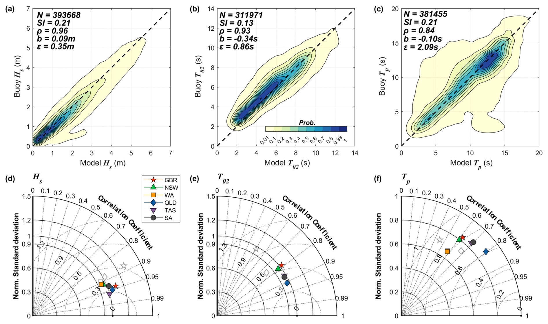
Figure 9 Comparison of the (a) significant wave height H_s, (b) mean period T₀₂, and (c) peak period T_p between a total of 28 wave buoys and the WW3-ST6 simulation Run 5 (with S_uo; Table 2). Taylor diagrams summarizing the comparison between Run 5 (colored, full markers) and buoys at different regions for (d) H_s, (e) mean period T₀₂, and (f) peak period T_p. For comparison, the gray, empty markers illustrate the performance of Run 4 (without S_uo) in the GBR (star), WA (square), and QLD (diamond) regions. Buoys are divided into groups according to Fig. 6.

Figure 10 presents the model performance (Run 5) in simulating wave heights and periods specifically at each wave buoy. The spatial distribution of model errors shown here is generally consistent with the altimeter-based analysis (Fig. 7c and d): wave heights are overestimated by 5 %–10 % along the coast of Western and Southern Australia and mostly underestimated by 5 %–10 % along the Eastern Australian coast, especially at buoys off the coast of New South Wales. A few buoys near Western Australia, particularly near Perth, show large model errors in H_s with biases higher than 1 m, forming the hook-like shape found in the lower-bottom corner of Fig. 7a. The WW3 Run 5 yields a 5 %–15 % underestimation in both T₀₂ and T_p along the eastern coasts but overestimates T_p moderately in the coastal waters of Western and South Australia. These large-scale error patterns are defined by the open-boundary wave spectra from our global simulations for which swells originating from the Southern Ocean were overestimated by around 5 % (Liu et al., 2021; their Fig. 8a).

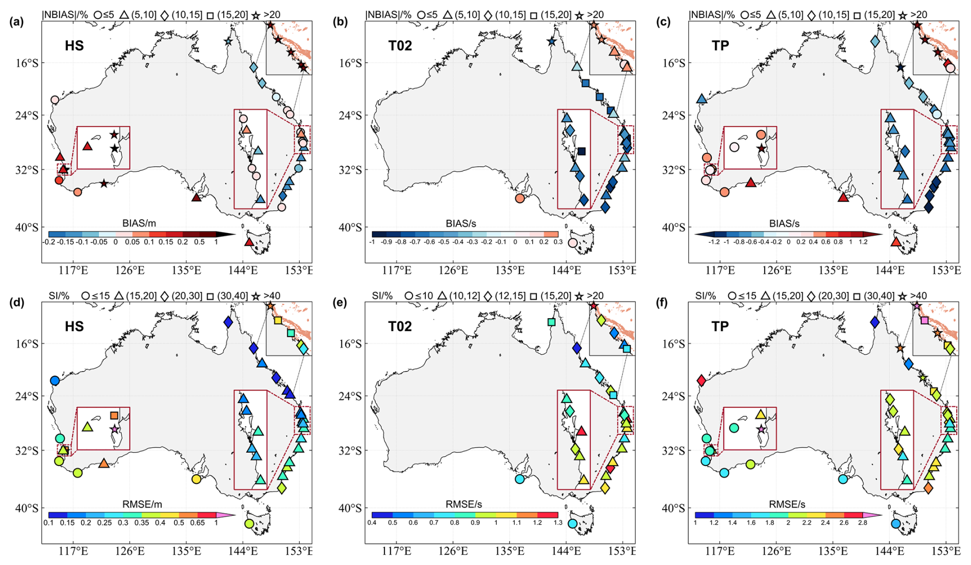
Figure 10 Comparison of the WW3-ST6 simulation (Run 5 with S_uo) against wave buoy observations in 2011 for (a, d) wave height H_s, (b, e) mean wave period T₀₂, and (c, f) T_p. The colors and symbols in panels (a)–(c) represent the bias b and normalized bias b_n (in %). The colors and symbols in panels (d)–(f) represent the RMSE and scatter index (in %). The enlarged views of buoys near Perth and Brisbane are given in the bottom-left and bottom-right insets. The inset in the upper-right corner shows the results at the GBR buoys from Run 4 (without S_uo).

The performance of Run 4 without S_uo at the GBR buoys is also given in the inset in the upper-right corner of Fig. 10a–c. All three wave parameters were seriously overestimated by this run at the five GBR buoys: the bias for H_s is more than 1 m, and the T_p bias is mostly above 1 s. The inclusion of S_uo in Run 5 clearly reduces the RMSE, in particular for H_s and T_p (Fig. 10d–f), and the model now generally underestimates these wave parameters by around 10 %–20 %.

To close this section, we present the time series of wave heights and wave periods at 55032, the shallowest one among the five GBR buoys, over a 2-month period (October–November 2011), providing the most visually intuitive confirmation of the benefit of S_uo. As seen, when the reef parameterization is not used, H_s and T_p from Run 4 are obviously biased high and are consistent with the results presented in Zieger and Peach (2023). On the contrary, Run 5 agrees with the buoy observations much more closely primarily because S_uo dissipates the overestimated incident swell energy to a reasonable level, bringing both H_s and T_p down to the buoy measurements. The results for mean wave period T₀₂ are less favorable, and Run 5 performs marginally better in terms of the SI and correlation coefficient (Fig. 11b). This may be related to the setting of the empirical coefficient ψ (Eq. 14), which could lead to an overestimation of the energy dissipation.

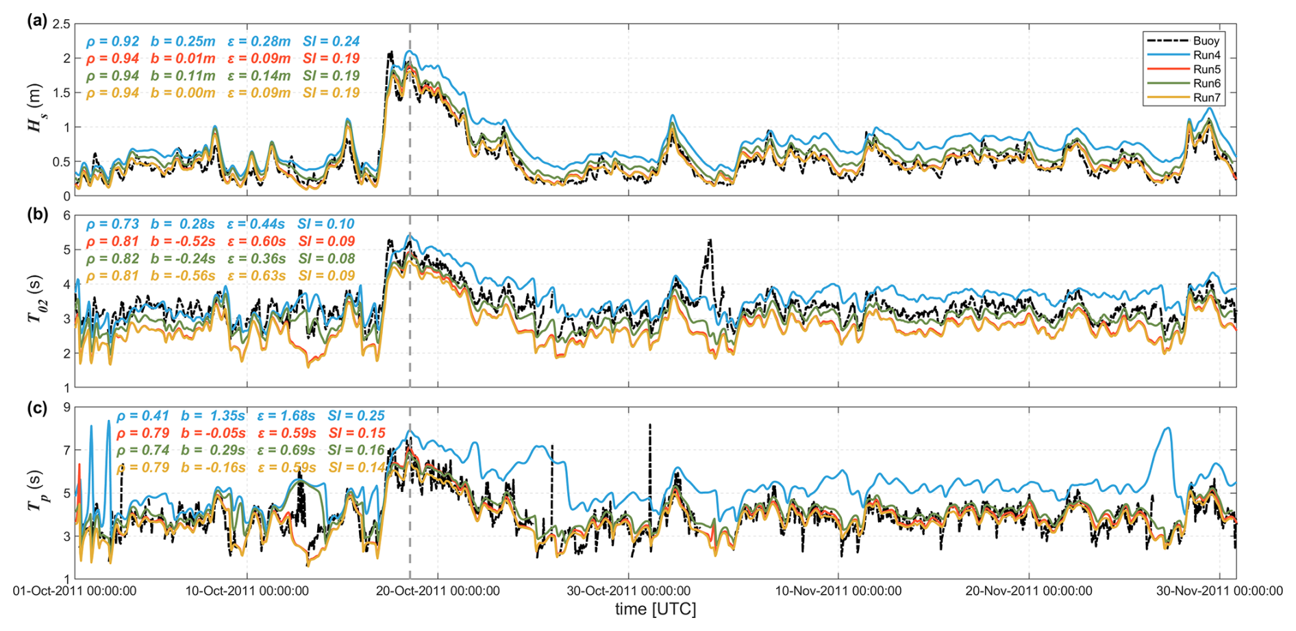
Figure 11 Comparison of the (a) significant wave height H_s, (b) mean period T₀₂, and (c) peak period T_p between observations and the WW3 simulations (Runs 4 and 5 used mesh v1, and Runs 6 and 7 used mesh v2; Runs 4 and 6 without S_uo, and Runs 5 and 7 with S_uo) for a 2-month period (October–November 2011) at Hay Point wave buoy (55032; water depth of 9 m). The error metrics for Runs 4, 5, 6, and 7 are printed in blue, red, green, and yellow, respectively. The vertical dashed line highlights the time instant analyzed in Fig. 12a–d.

5 Discussions

5.1 Source term balance

The striking improvement led by the subgrid-scale reef parameterization in the GBR, as shown in the previous section, indicates the possible predominance of the coral-reef-induced dissipation over other physical processes. In this section, we present a thorough analysis of the source term balance in the GBR, illustrating the relative precedence of different source terms in this complex context and explaining why the reef parameterization is effective within our km-scale modeling framework.

Figure 12 shows directional wave spectra F(f, θ) from two different WW3 simulations (i.e., Run 4 without S_uo and Run 5 with S_uo) at buoy 55032 at 13:00 UTC 18 October 2011, when the simulated wave height reaches the maximum (∼ 2 m) during the 2-month period, as shown in Fig. 11. The corresponding 1D spectra and source terms (normalized by the spectrum) produced by WW3 are also given. For this specific time instant, it is seen that S_uo gives rise to a significant reduction in wave height (from 2.10 to 1.88 m), yielding closer agreement with the buoy observation (1.97 m; Fig. 12b). Most of the reduction in wave energy is observed at low frequencies, especially around the spectral peaks. This is partially dictated by the reduction factor formulated in Eq. (14). The peak wave direction θ_p, however, is only marginally affected by S_uo (Fig. 12a).

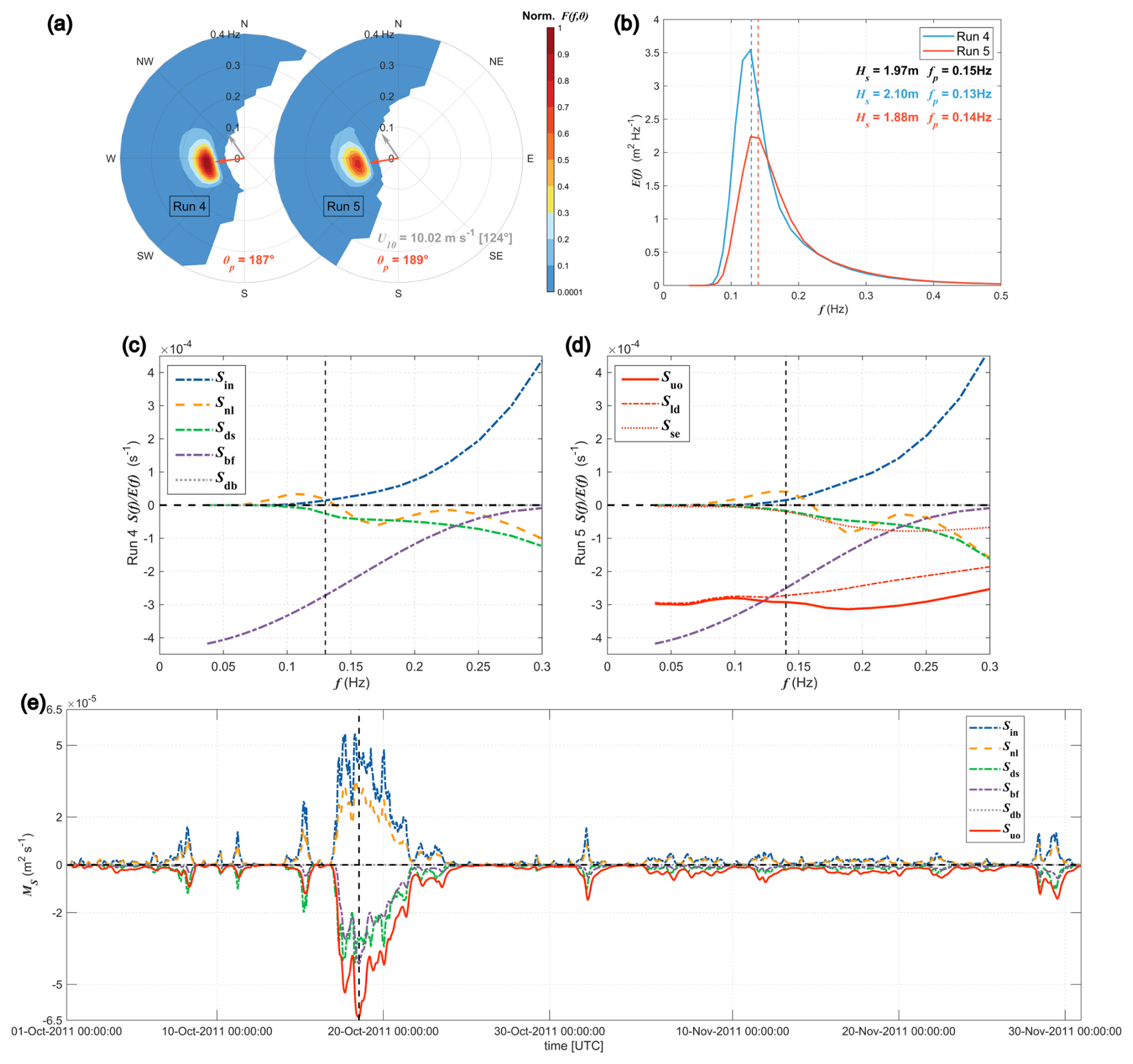
Figure 12 (a) Wave spectra F(f, θ) at buoy 55032 at 13:00 UTC 18 October 2011 from Run 4 (without S_uo) and Run 5 (with S_uo). The gray and red arrows denote wind and peak wave directions. (b) The corresponding 1D wave spectra E(f) with the respective wave height H_s and peak frequency f_p. Buoy observations are shown in black. (c, d) The corresponding source terms, each normalized by the spectra from Run 4 (without S_uo) and Run 5 (with S_uo), respectively. In panel (d), the unresolved obstacle-related parameterization S_uo, together with the separate local dissipation (S_ld) and shadow effect (S_se), is shown by the red lines. Evolution of the source term magnitude M_S at 55032 for the 2-month period is shown in panel (e). Note that when calculating S_uo, the transparency coefficients (α, β) and path length ΔL at the node closest to the buoy station were used. The vertical dashed lines in (b)–(d) represent locations of the peak frequency, whereas the vertical dashed line in (e) illustrates the time instant for the spectra shown in (a).

When S_uo is not taken into account (Fig. 12c), the bottom friction S_bf represents the strongest source term at this shallow-water buoy, dissipating wave energy in the energy-containing frequency range (e.g., f<0.2 Hz; Fig. 12c). The wind input S_in, wave breaking S_ds, and four-wave nonlinear interaction S_nl are basically comparable to each other and are markedly lower than S_bf in the peak region. Nonetheless, as expected, the wind input term becomes dominant in the high-frequency range. In Run 5 with S_uo included, the normalized bottom friction term remains unchanged because the water depth does not change in these two different runs. However, the most important result is that, in this case, the dissipation owing to unresolved obstacles S_uo is comparable to, or even larger than, S_bf. A careful examination of S_uo shows that the dissipation is mainly attributed to the local dissipation S_ld rather than the shadow effect S_se for this specific buoy location. At the buoy considered (d=8.97 m), the fraction of breakers Q_b (Eq. 10) becomes significant (>1 %) only for H_s>4.3 m. For the values of H_s shown here and in Fig. 11, the depth-induced wave breaking S_db is therefore always negligible.

Finally, to investigate the strength of all the source terms throughout the entire 2-month period shown in Fig. 11, we calculated the source term magnitude by adopting the definition introduced by van Vledder et al. (2016). For a given source term S_S, its magnitude M_S is defined as

$$\begin{array}{}\text{(16)}& M_{\mathrm{S}}=sgn\left(S_{\mathrm{S}}\right)\int \int \left|S_{\mathrm{S}}(f,\mathit{\theta })\right|\mathrm{d}f\mathrm{d}\mathit{\theta },\end{array}$$

where the sign function assures that the magnitude of the dissipative source terms is always negative. Absolute values are used for the integrand so that the importance of the nonlinear interaction term S_nl could be better recognized. Otherwise, the integral of S_nl over frequency is always nearly zero (e.g., Rogers et al., 2012, their Fig. 7). The temporal evolution of source term magnitudes at buoy 55032 during October–November 2011 is given in Fig. 12e. It is obvious that the two most dominant physical processes are the dissipation owing to unresolved reefs (S_uo) and the input from winds (S_in). However, because the S_in magnitude is primarily attributed to short waves in the high-frequency range (e.g., f>f_p), the dissipative S_uo term is therefore more effective in modulating wave energy in the energy-containing range, again reflecting its predominant role in shaping the wave spectrum at this buoy station.

It should be stressed that the purpose of analyzing the source term balance here is to demonstrate the added value of S_uo in parameterizing wave dissipation induced by coral reefs when these reefs are not really resolved by our km-scale wave models. Undoubtedly, in the real oceans or for wave simulations at much higher resolutions (e.g., meter scale) in which reefs and their surrounding bathymetry are much better resolved, the magnitudes of different source terms, particularly the bottom friction and depth-induced breaking terms, could change significantly owing to the usage of more realistic water depths.

5.2 Sensitivity to the grid resolution

Thus far, the results shown are all based on our relatively coarse grid, in which the resolution around the GBR is about 5–10 km (mesh version 1 in Table 1; Fig. 2b). Naturally, one may ask how much the model performance and S_uo are sensitive to the grid resolution. To answer this question, we designed another more refined mesh, with the grid size around the GBR increased to approximately 1 km (Fig. 13). Consequently, the total numbers of nodes and elements have increased by more than double in this new grid system (mesh version 2 in Table 1).

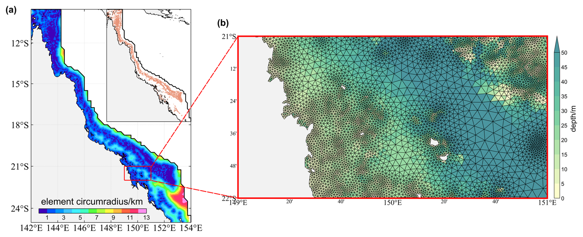
Figure 13 (a) The mesh resolution (in terms of the local element circumradius; unit: km) of mesh version 2 (details in Table 1) zoomed in around the GBR. (b) A triangular grid (mesh v2) with varying resolutions, zoomed in at a 1°×2° bin off the northeast coast of Australia.

Model results at wave buoy 55032 based on this new mesh (i.e., Runs 6 and 7 in Table 2) are presented in Fig. 11 as well. At this station, when S_uo was not included, the higher-resolution simulation (Run 6) performs much better than the coarser one (Run 4), with the H_s bias reduced from 0.25 to 0.14 m. Nonetheless, with the same time steps used, Run 6 is ∼50 % more expensive than the coarser runs (Runs 4 and 5). Moreover, in terms of the wave height accuracy, Run 6 is still not as good as Run 5 (with S_uo). This is not surprising because we showed in Fig. 2a that even the 1 km grid can resolve only ∼40 % of reef polygons for the GBR. When S_uo is considered, it is encouraging to see that simulations at two different resolutions (Runs 5 and 7) are practically the same at buoy 55032, indicating that even the grid resolution increases considerably in Run 7; S_uo does not bring too much excessive dissipation, at least for the km-scale wave simulations investigated here. We note that, however, when compared against altimeters, the wave height from Run 7 indeed is 5 %–10 % lower than that from Run 5 for most of the GBR, and the magnitude of S_uo may also vary significantly between Runs 5 and 7 owing to changes in their respective transparency coefficients (α and β; Sect. S6). Despite this, our km-scale simulations with S_uo are apparently superior to simulations without S_uo (Runs 5 and 7 vs. Runs 4 and 6), demonstrating the good applicability of S_uo to wave simulations of the GBR at km scale (i.e., 1 km and higher).

5.3 Other uncertainties in the wave simulations

In addition to the factors explicitly evaluated in this study, several other sources of uncertainties may influence the model results. First, uncertainties may arise from the coral reef data. As detailed in Sect. 2.3, reef outlines were extracted from the multi-source global coral reef dataset (UNEP-WCMC et al., 2010) to calculate the transparency parameters α and β in the GBR. However, these outlines may represent reef platforms rather than actual reef canopies, which could introduce uncertainties into the real geographical locations of reefs and thus into the model results.

Secondly, uncertainties may also arise from the empirical coefficients used in the model framework, particularly the correction factor ψ (Eq. 14) and the drag coefficient employed in ST6. The correction factor ψ was introduced into the UOST scheme based on previous theoretical arguments and modeling experiences (Mentaschi et al., 2015, 2018). However, due to the lack of dedicated spectral observations in the proximity of both the upstream and downstream islands and reefs, its validity has not yet been thoroughly evaluated. In addition, the drag coefficient used in ST6, which follows the work of Hwang (2011), was originally developed based on open-ocean observations. While our results indicate that the ST6 (without any tuning) performs reasonably well in shallow coastal environments, the representation of the drag coefficient and wind stress could be further improved.

Finally, it is important to note that the two-step modeling methodology was developed based on the GBR. However, coral reef systems also include fringing or land-backed reefs directly attached to coastlines or islands, such as those in the Philippines. In these cases, because the reefs are closely connected to land, their additional capacity to dissipate wave energy may be relatively limited. Therefore, the improvements from applying our scheme may be less significant in these areas, where the reef's role in wave energy dissipation is less pronounced compared to offshore, structurally complex reef systems like the GBR.

6 Concluding remarks

A series of 1-year numerical simulations of ocean surface waves around the Australian coast were performed in this study, using the spectral wave model WW3 and the state-of-the-art physics and numerics. For better resolving the extensive Australian coastline, we generated a national-scale, high-resolution unstructured mesh with approximately 90 000 nodes and 160 000 elements, of which the spatial resolution ranged from 1 km at the coastline to 15 km at open boundaries (Fig. 1). The wave model results are thoroughly compared and validated against altimeter data and in situ wave buoy observations. Key findings of this study are summarized below:

Overall, the WW3-ST6 physics (Liu et al., 2019), together with other relevant source terms, performs reasonably well in the Australian coastal waters, showing a bias of H_s mostly within 10 % and a bias of T₀₂ and T_p generally less than 15 % (Figs. 7 and 10). A notable exception is the GBR region, in which wave energy is severely overestimated (>100 %) because the local mesh fails to resolve those numerous but also fairly small individual reefs (Fig. 2), and thus the dissipative effects of coral reefs could not be simulated explicitly.

To improve the model accuracy in the GBR, we regarded the individual reefs as unresolved obstacles (islands) in the mesh, assuming that coral reefs behave as total barriers to wave energy, and then adopted the UOST parameterization of Mentaschi et al. (2018) to estimate the energy dissipation induced by these subgrid-scale obstacles (Figs. 4 and 5). It was confirmed that this two-step modeling strategy reduces model errors of wave heights and periods in the GBR dramatically (Figs. 8–11), demonstrating its striking benefit for wave simulations in this challenging area.

Further analysis of the source term balance in the shallow water of the GBR (Fig. 12) corroborates the important role of the subgrid-scale dissipative parameterization S_uo as a proxy for the coral-reef-induced dissipation. This once again necessitates the use of a reef parameterization in numerical wave modeling in this specific context (i.e., km-scale or even coarser-resolution wave simulations around the GBR) in which individual coral reefs could not be well resolved, as already discussed by previous studies (Hardy et al., 2000).

In conclusion, this paper builds upon the modern physics and numerics of WW3, clearly demonstrating its applicability and reliability in simulating ocean waves in the Australian coastal waters and even in the complex reef matrix. It is therefore expected that our study would benefit future research and applications related to Australian wave forecasting (Zieger and Peach, 2023) and hindcasting (e.g., Zieger et al., 2019), ocean engineering design, and wave climate (e.g., Hardy et al., 2000). It is known that ocean waves play a crucial role in determining coral reef ecology. The findings given here might also be useful for numerical research on the complex physical and biological feedbacks involved at coral reefs (Lowe et al., 2005; Lowe and Falter, 2015).

Appendix A

The ACCESS currents mentioned in Sect. 3.4 did not account for tides (Kiss et al., 2020). As pointed out by one of our reviewers, tides modulate water depth and surface currents and therefore may impact the overall results significantly, particularly in the GBR. In order to check the impact of tides on our modeling results, we conducted another 2-month run by including the tidal elevation and currents (i.e., Run 8 in Table 2) derived from the FES2014 dataset (1/16° and 1 hourly; Lyard et al., 2006, 2021). Owing to its refined bathymetric models and optimized assimilation schemes, the FES2014 tides dataset was extensively used along the Australian coast and in the vicinity of the Great Barrier Reef (Cancet et al., 2017; Carrere et al., 2015; Seifi et al., 2019).

Figure A1 depicts the time series of wave parameters, tidal elevation, and tidal currents for October 2011 at 55032. The model depth is 8.97 m, and the tidal elevation range varies from −2.98 to 3.21 m in this period. Statistically, the overall performance of Run 8 (with tides) over this month is nearly identical to that of Run 5 (without tides). Validations against altimeter wave observations show marginal differences in these two runs as well (Fig. S9). There is no doubt that, in practice, wave heights on reef crests are strongly modulated by the tidal elevation, as we mentioned in Sect. 2.3. However, in the context of our km-scale (or even coarser-resolution) wave modeling covering the entire Australian coastline, most of the reefs could not be resolved and are modeled as subgrid “islands”. Consequently, for our wave simulations at these spatial scales, it becomes impractical to discuss tidal modulations of wave heights on reef crests. For a similar reason, the inclusion of the FES2014 tides did not lead to significant changes in the overall monthly and yearly error metrics. Despite this, we note that the tidal modulation of wave parameters is still noticeable on the daily timescale, particularly for wave periods during 20–30 October (Fig. A1b and c), when waves were relatively longer.

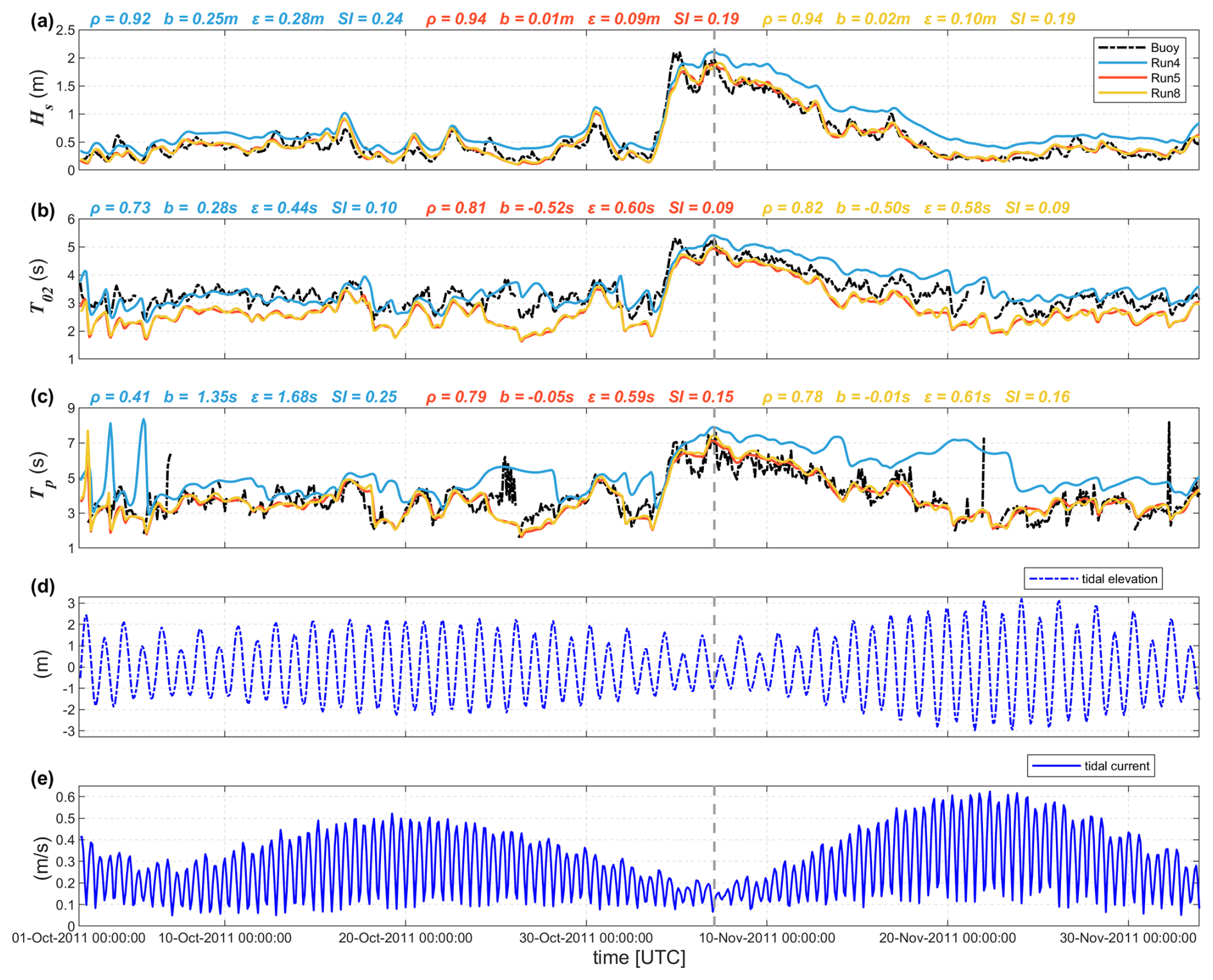
Figure A1 Comparison of the (a) significant wave height H_s, (b) mean period T₀₂, and (c) peak period T_p between observations and the WW3 simulations (Run 4 without S_uo and tides, Run 5 with S_uo but without tides, and Run 8 with S_uo and FES2014 tides) during October 2011 at Hay Point wave buoy (55032; water depth of 9 m). The error metrics are printed in blue, red, and yellow, respectively. (d) and (e) represent the tidal elevation and tidal currents for October 2011 based on the FES2014 database, respectively. The vertical dashed line highlights the time instant analyzed in Fig. 12.