the Creative Commons Attribution 4.0 License.
the Creative Commons Attribution 4.0 License.
 | 05 Sep 2025
PALM-SLUrb v24.04: a single-layer urban canopy model for the PALM model system – model description and first evaluation
Matthias Sühring
Ewan O'Connor
Leena Järvi
Urban areas are recognised as critical zones for climate research due to the high number of people living in these areas and their significant impacts on local and regional climates. However, understanding urban boundary layer processes remains a challenge, as existing mesoscale models cannot resolve their fine-scale features and dynamics, while microscale fluid dynamics simulations remain computationally expensive or unfeasible for the full extent of the urban atmosphere. To address this gap, we present PALM-SLUrb, a single-layer urban canopy model for the PALM model system, offering a computationally efficient and physics-based model to represent urban surfaces on non-building-resolving grids. Together with the model description, we present sensitivity tests and a model comparison against grid-resolved urban canopies to demonstrate the model's performance. The results demonstrate the model's ability to extend the representation of key urban–atmosphere interactions in PALM to coarser grid resolutions on the order of 10 m. By bridging the gap between computational efficiency and physical detail, PALM-SLUrb broadens PALM's capabilities in advancing urban climate research.
- Article
(3589 KB) - Full-text XML
- BibTeX
- EndNote


Urban areas are increasingly a major focus of climate research due to their significant impact on local and regional climates. The complex interaction between highly variable urban surfaces, atmospheric dynamics, and human activities creates a higher spatial and temporal variability in the physical state of the atmosphere close to the surface, relative to rural environments (Oke, 1987; Arnfield, 2003; Stewart and Oke, 2012). Understanding the flow and transport processes in the urban boundary layer (UBL) is crucial for addressing challenges related to urban heat islands, air quality, regional to hyperlocal weather forecasts, and energy consumption (Grimmond et al., 2010; Masson, 2006). However, as highlighted in a review by Barlow (2014), the UBL is one of the most complex and least understood parts of the atmosphere, requiring detailed studies across a range of scales from micro- to mesoscale. The heterogeneity in urban surface characteristics, combined with dynamic human-induced modifications to the atmosphere, presents significant challenges for both modelling and observations (Martilli et al., 2002; Best and Grimmond, 2015).
Our understanding of urban-specific phenomena at fine spatial and temporal scales and their interaction with mesoscale dynamics remains limited. Mesoscale numerical weather prediction models, with their coarser resolutions, cannot adequately resolve the finer-scale flow and transport processes characteristic of the UBL. Conversely, microscale simulations, including large-eddy simulations (LESs), while capable of capturing these small-scale urban features, are computationally prohibitive for covering large urban areas and often neglect the influence of larger-scale mesoscale phenomena with horizontal scales of tens or even hundreds of kilometres (Martilli et al., 2002; Barlow, 2014). This scale gap highlights the need for modelling approaches that integrate processes across scales to improve our understanding of the UBL. Developing such model systems will enable researchers and city planners to devise more effective strategies for mitigating adverse urban climate effects and advancing sustainable urban planning (Krayenhoff et al., 2021).
The PALM model system (PALM for short; Raasch and Schröter, 2001; Maronga et al., 2015, 2020) is an actively developed and comprehensive atmospheric and oceanic modelling system for boundary layer flows. It is most widely known for high-resolution large-eddy simulations (LESs) of the UBL and for excellent scaling in modern high-performance computing (HPC) environments. PALM is written in a modern Fortran standard (Fortran 2003) and is freely available under the GNU General Public Licence v3.0 (GNU GPLv3).
The implementation of Cartesian topography (Maronga et al., 2015, 2020), a land surface model PALM-LSM (LSM for short; Gehrke et al., 2021), a building surface model PALM-USM (USM for short; Resler et al., 2017) and a radiative transfer model (RTM; Krč et al., 2021) has enabled the explicit representation of three-dimensional grid-resolved urban surfaces and canopies in PALM simulations. With this grid-resolved urban canopy approach, surface fluxes of radiation and heat are computed by solving the surface and subsurface energy balances for each of the atmosphere-facing cell faces in the prescribed topography, with local subgrid-scale momentum flux modelled using the surface resistance approach. Moreover, the pressure drag from grid-resolved obstacles (e.g. buildings) is implicitly taken into account by the application of the topography masking method in pressure solvers. This grid-resolved urban canopy approach expects the urban form to be adequately represented in the simulation grid in all three spatial dimensions.
Furthermore, as this approach is targeted only to be used with building-resolving grids, it poses an underlying approach that the atmospheric model and the radiative transfer model should be capable of accurately modelling the atmospheric transport processes within the urban canopy. With a rough approximation that, in LES, the grid resolution should not exceed of a typical surface feature (e.g. a single street canyon or building) so that the turbulent transport processes within the cavities, such as street canyons, are still represented with a reasonable accuracy, grid resolutions of 1 to 2 m or even finer are typically required, with urban canopies of typical packing densities (see e.g. Xie and Castro, 2006). Thus, although we refer to this approach as a resolved urban canopy approach, it depends heavily on the grid resolution how well the canopy and the processes within the canopy are actually represented and resolved in a simulation.
Employing physical domain sizes large enough to include these mesoscale phenomena together with the metre-scale grid resolution required for the resolved urban canopy approach leads to domain sizes that are not computationally feasible. In order to bridge the gap between meso- and microscales in urban studies, the self-nesting system of PALM can be applied (Hellsten et al., 2021). With the nesting strategy, coarser-resolution simulation domains, still capable of resolving the larger-scale atmospheric phenomena, provide the turbulent boundary conditions for the high-resolution inner domain covering the urban area of interest.
However, even with the self-nesting system, the computational costs for representing large urban areas at the building-resolving scale remain high. Furthermore, for medium-to-large-size cities, the urban area may extend well beyond the limits of the finer-resolution nested domains, potentially leading to insufficient surface representation in the upwind direction of the study area.
In many studies, where the focus is not the urban canopy itself, simulating the urban boundary layer at metre-scale resolution and representing the urban canopy in high detail might not even be necessary. For example, 𝒪(10 m) grid spacings may already be sufficient to explicitly resolve nearly all of the anisotropic turbulence in a convective boundary layer (Sullivan and Patton, 2011; Wurps et al., 2020). The resolution requirement of explicitly resolving the urban canopy flow can therefore severely limit the feasibility of utilising PALM for such applications.
To provide an alternative urban surface representation in PALM, we present a newly developed single-layer urban canopy model, PALM-SLUrb (SLUrb for short). The main purpose of the new model is to produce urban surface forcing and neighbourhood-scale bulk urban meteorological conditions comparable to the high-resolution resolved canopy approach but with non-building-resolving grids. The model formulation of SLUrb is based on the single-layer version of the Town Energy Balance (TEB) model (e.g. Masson, 2000; Lemonsu et al., 2013) as implemented in the SURFEX model v8.1 (Le Moigne, 2018). When selecting the basis model, several criteria were considered: the primary criterion was to select a well-known, evaluated model with a reasonable pre-existing user base; second, a model that models turbulent transport using aerodynamic resistances was preferred for consistency, as this resistance-based approach is also used in PALM's pre-existing surface models; third, a model with a set of inputs that are generally available and commonly used in urban climatological studies was required; and, finally, a model with licensing compatible with the GNU GPLv3 licence was preferred, although no code base was eventually shared.
The decision to select a relatively simple urban canopy representation instead of a more complex one was supported by the findings from prior urban land surface model intercomparison and evaluation projects (Grimmond et al., 2010; Lipson et al., 2024). These findings suggest that the more complex models do not necessarily perform any better than the simpler ones in metrics related to the modelled surface forcing. Furthermore, as PALM already provides a possibility for a highly detailed urban representation with the resolved urban canopy approach, a simpler model was preferred for an alternative.
As the aim was to implement a model that interactively couples with the turbulence-resolving LES without any temporal aggregation, coupling the pre-existing TEB model with the atmospheric model was deemed technically unpractical or even unachievable. Thus, a novel implementation of a newly written surface model, based on TEB model formulation and equations, integrated into an LES model, was written. Additionally, developing the model code base from scratch allowed for utilising the pre-existing module framework and interfaces of PALM, with similar data structures, parallelisation strategy, I/O routines, and numerical schemes used as in other PALM modules. Due to extensive differences in the model formulation, technical implementation, and numerical schemes, SLUrb should not be considered an integration of TEB in PALM but rather an independent model tailored specifically for PALM.
Based on publicly available records, there are only a few models that currently implement coupling of an LES with an urban canopy model. The Advanced Research WRF (ARW) configuration of the Weather Research and Forecasting (WRF) model (Skamarock et al., 2019) provides coupling with the LES mode (WRF-LES) and a single-layer urban canopy model (UCM; Kusaka and Kimura, 2004), whereas the multi-layer Building Energy Parameterisation (BEP) model is not supported in LES mode. Additionally, there exists a variant of WRF-ARW with coupling to the TEB model (Meyer et al., 2020). The Icosahedral Nonhydrostatic (ICON) model (Zängl et al., 2015; Giorgetta et al., 2018) in its large-eddy model configuration (ICON-LEM; Heinze et al., 2017) implements a coupling of an LES with the TERRA_URB urban canopy scheme (Campanale et al., 2025), although, at the time of writing, no peer-reviewed studies combining the two exist.
While WRF-LES has been successfully applied in several urban studies at 𝒪(100 m) grid resolutions (e.g. Zhu et al., 2017; Huang et al., 2019; Udina et al., 2020; Pinto et al., 2021), only a few studies (e.g. Zhong et al., 2020; Wang et al., 2023) have extended to finer 𝒪(10 m) grid resolutions. Thus, there is still a need for further urban studies at these resolutions that bridge the range of resolutions lying between pre-existing approaches.
This article presents the first version of the PALM-SLUrb model as implemented in PALM model system version 24.04, along with sensitivity experiments and a model comparison against PALM simulations with LES-modelled urban canopies. Section 2 provides an extensive physical and technical description of the model and its implementation. This is followed by an analysis of the model sensitivity against internal model parameters and external forcing in Sect. 3. In Sect. 4, a model comparison experiment against PALM simulations with resolved urban canopies at varying grid resolutions is presented. Finally, key limitations and a development outlook of the model are discussed in Sect. 5, followed by concluding remarks.
2.1 Overview
Following TEB's concepts, SLUrb represents urban canopy in two dimensions using an infinite canyon assumption, with energy balances of roofs, walls, windows, and roads (jointly referred to as SLUrb surfaces or simply surfaces in the model description) solved separately. These surfaces are interconnected to each other and to the atmosphere by a network of resistances, modelling the transport of heat, both sensible and latent, within urban canopy as well as between the urban canopy and the first atmospheric model level. As SLUrb models the urban canopy and roughness layers, where the flow is directly influenced by individual roughness elements, the fluxes entered at the first atmospheric model level are grid-average fluxes. Thus, they represent the resulting surface layer fluxes where these direct influences of these roughness elements for airflow and heat transport have blended together. The atmospheric model is then responsible for modelling only the upper part of the surface layer.
Roofs are represented as one single flat surface per urban tile, experiencing no shading from the urban canopy. For canyon systems, the radiative processes, including shading and trapping of radiation within the urban canopy, are parameterised using an internal radiation model. Momentum flux is modelled for the urban surface as a whole using urban roughness parameterisation. SLUrb provides isotropic and anisotropic versions of the canyon model, meaning that canyons with or without a specific orientation can be modelled. As SLUrb is a single-layer canopy model, the internal conditions in the canyon are modelled only at canyon half-height regardless of the resolution of the atmospheric simulation. A schematic overview of the geometry and the physical processes represented by the model is provided in Fig. 1.
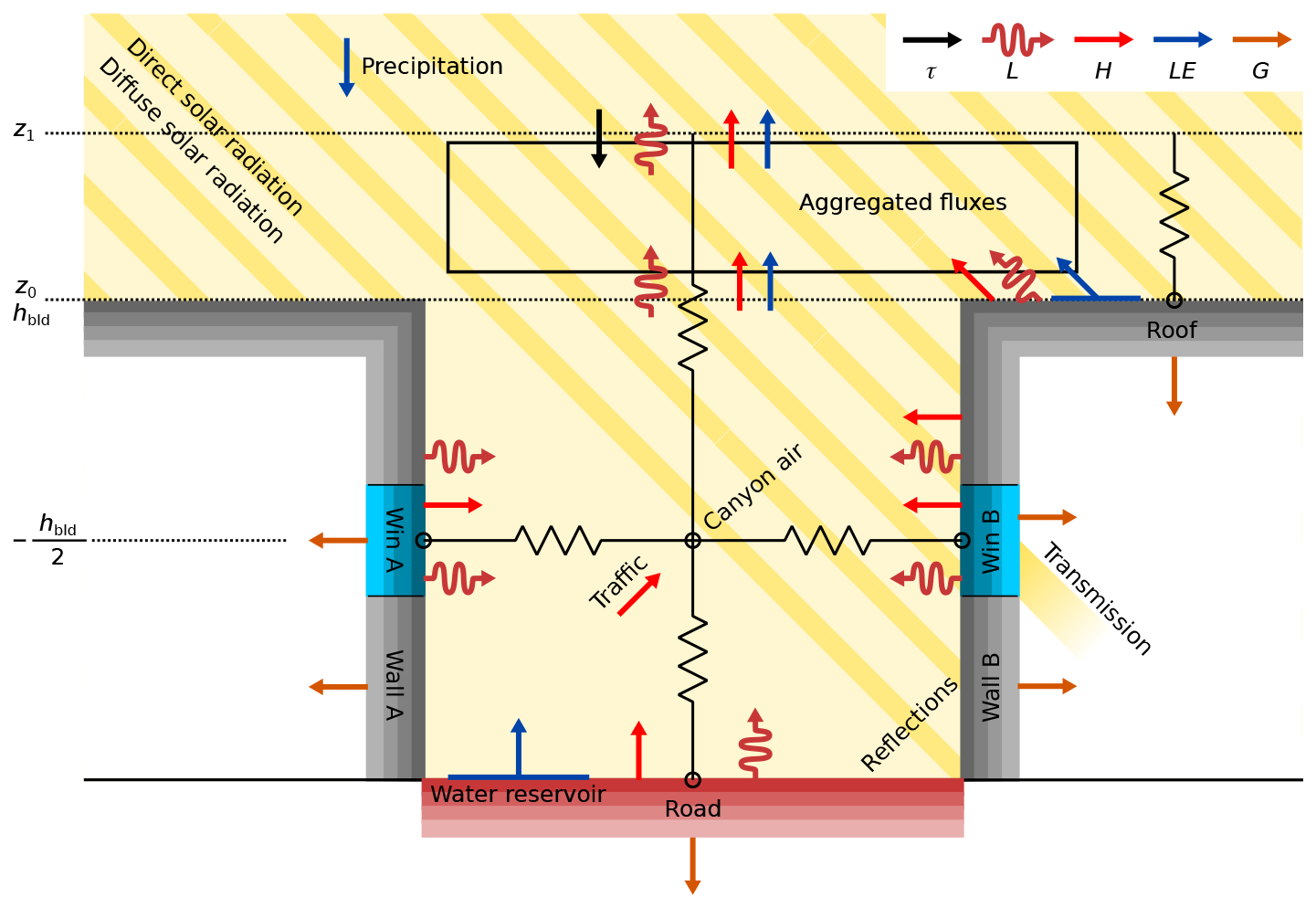
Figure 1A schematic overview of the physical processes included in SLUrb, where τ represents parameterised momentum fluxes, L denotes longwave radiative fluxes, H denotes sensible heat fluxes, LE represents latent heat fluxes, and G denotes conductive heat fluxes. The modelled resistance network is illustrated with resistor symbols (lines with a zigzag segment). The surfaces are illustrated with the default four material layers. Note that only one roof surface per urban tile is modelled.
The model is interactively coupled to the atmospheric simulation at each time step. The heat exchange with the first atmospheric level is solved separately for roofs and canyon systems, whereas the momentum transport is not explicitly modelled for the SLUrb's internal surfaces but rather for the aggregate urban surface as a whole (see Sect. 2.7.2 on model coupling). The surface grid cells combine both SLUrb (urban) and LSM (vegetation or water) tiles to provide total surface–atmosphere exchange.
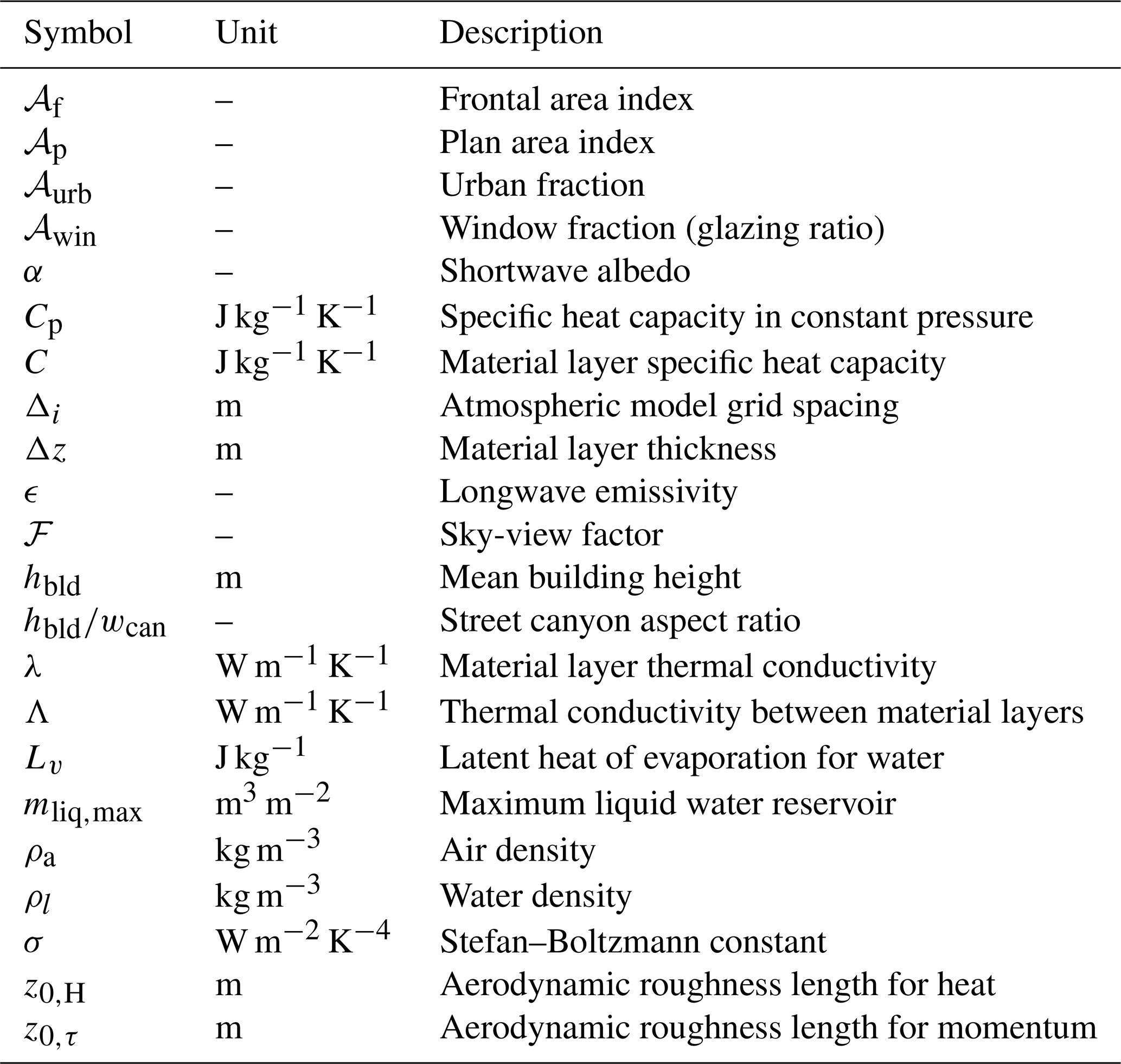
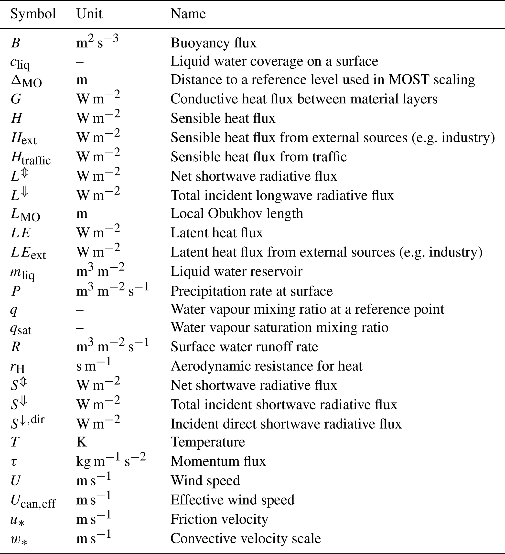
The individual model components are individually described in the following subsections, with the sectioning roughly following the modularisation of the model code. For reference, a nomenclature of model parameters and another for variables are listed in separate tables (Tables 1 and 2, respectively).
Table 1Nomenclature of the model parameters and constants in SLUrb that are either given as an input or set by the atmospheric model.
2.2 Energy balance on surfaces
The surface energy balance equation SLUrb solves for each surface, written in general form for a given surface indicated with ⋆, and is defined as
where is the temperature of the material layer closest to the surface, is its heat capacity, and are the net shortwave and longwave radiation budgets modelled by an internal canopy radiation model, H⋆ is the surface sensible heat flux, LE⋆ is the surface latent flux, and is the conductive heat flux to the second material layer. To model subsurface heat conduction, a one-dimensional discrete heat diffusion equation is solved for subsurface temperatures , where k>0 is the index of the subsurface layer (see Sect. 2.6 for details). LE⋆ is considered only for horizontal surfaces, i.e. roofs and roads. For walls and windows, LE⋆ is omitted from the surface energy balance. Both sensible and latent fluxes are computed between the surface and a reference point, the reference point being the first atmospheric model level for roofs, and the canyon midpoint for walls, windows, and roads. The sensible heat flux between a given surface ⋆ and its corresponding reference point is modelled using the bulk transfer equation:
where ρa is the density of air, Cda,p is the specific heat capacity of dry air under constant pressure, is the aerodynamic resistance (hereafter simply resistance) for the heat transfer, and is the air temperature at the reference point.
In SLUrb, horizontal surfaces can be either dry, partially covered by liquid water, or fully covered. The full surface area is used for condensation and precipitation interception, whereas evaporation is possible only from an area covered by liquid water. Thus, parameterisation for the latent heat flux depends on saturation at the surface and is defined in SLUrb as
where Lv is the latent heat of evaporation, is the coverage of liquid water on the surface, is the water vapour mixing ratio at the reference point, and is the water vapour mixing ratio at saturation at the surface. Computation of requires solving a prognostic equation for the liquid water reservoir on the surface:
where ρl is the density of water, P is the precipitation rate on the surface as provided by the atmospheric model, and R is surface runoff. The maximum liquid water reservoir mliq,max is set to 10−3 m−3 m−2 following Masson (2000), equivalent to a 1 mm layer of liquid water. Runoff is directly computed as the amount of water needed to be removed from the reservoir to bring it within the limit of mliq,max. The runoff is assumed to enter drainage systems and thus is removed from the model. Finally, is computed following Noilhan and Planton (1989) as
Integrating the model components results in a closed energy balance representing the complete SLUrb model system:
where 𝒜p is the plan area index (i.e. fraction of area occupied by buildings to the total plan area), is the street canyon aspect ratio, and 𝒜win is the window fraction (i.e. fraction of area occupied by windows to the total building facade area, also known as the glazing ratio). The terms in group (a) represent the aggregated atmosphere–urban fluxes, (b) additional fluxes that can be given as model inputs (with Hext and LEext being sensible and latent heat fluxes from external, typically anthropogenic sources not included in the model itself and Htraffic being the sensible heat flux from traffic that enters the canyon system), (c) the canyon system, (d) the roof, (e) the walls, (f) the windows, (g) the road, and (h) the moist physical processes. At each time step, SLUrb computes a solution for the set of prognostic variables (Tcan, qcan, Tk,roof, , , , , mroof,liq, and mroad,liq, with A and B referring to facades, as illustrated in Fig. 1) that fulfils the energy balance up to the accuracy of numerical schemes (10−3 … 10−6 W m−2 depending on, e.g., the time step of the atmospheric radiation model).
2.3 Canopy radiation model
To represent radiative processes within the urban canopy, SLUrb implements an internal urban canopy radiation parameterisation. The tile-averaged incident radiation partitions from a given atmospheric radiation model are directly taken as inputs, after which the radiative budgets of each surface in SLUrb are internally computed, with the resulting aggregated outgoing fluxes fed back into the atmospheric model (see Sect. 2.7.2 on model coupling for further details). Reflections and trapping are taken into account for the surfaces within the canyon following either the isotropic (Masson, 2000) or anisotropic (Lemonsu et al., 2013) version of TEB radiation parameterisations. The main difference with respect to Lemonsu et al. (2013), in addition to several differences in the technical implementation, is that the SLUrb version of the radiation model adds windows but omits gardens at this point. Similarly, the isotropic version following Masson (2000) is amended with window fractions on facades.
2.3.1 Shortwave radiation
The shortwave parameterisation includes contributions from direct and diffuse shortwave flux incident on the urban tile, which are further partitioned into SLUrb surfaces based on the canyon geometry, solar azimuth ϕsol, and zenith angles λsol. The total absorbed shortwave radiation is computed based on an analytical solution for infinite reflections as derived by Lemonsu et al. (2013). Given an anisotropic canyon with a prescribed orientation ϕcan, the incident direct solar radiative fluxes on the model surfaces are
where is the incident direct shortwave radiation on the urban tile and δϕ is an indicator function depending on which one of the walls is directly illuminated by the sun:
The windows are assumed to be evenly distributed across the facades, allowing the same incident fluxes to be used for both the walls and windows. Hence, we do not report the incident fluxes separately for walls and windows here. Note that a small error in the original Lemonsu et al. (2013) article has been corrected in the definition of , with multiplication instead of division by the sine function. For isotropic canyons, the incident fluxes are averaged over all canyon orientations, resulting in
where
is a critical canyon angle before averaging (see Masson, 2000, for details).
The calculation of incident diffuse shortwave radiation on the surfaces is based on sky-view factors. Roofs are assumed to have unobstructed view of the sky (ℱroof=1), whereas sky-view factors for roads and facade surfaces are based on canyon geometry following Masson (2000):
The total incident shortwave radiative fluxes from the sky before reflections on the surfaces are subsequently
where is the incident diffuse shortwave radiative flux from the sky on the urban tile.
Modelling a single reflection for the roofs and infinite reflections for the canyon surfaces, adapting the derivation by Lemonsu et al. (2013) in the context of SLUrb, leads to the final net shortwave radiation balances for the surfaces:
where is the aggregate shortwave albedo for facades and ℛfac is the mean facade reflection, defined as
For isotropic canyons, a mean of and is used for the average wall shortwave radiation balance . This solution is obtained by applying , a condition that follows directly from Eqs. (9) and (12), to the balance equation of either wall A or B.
As the incident radiation on windows is the same as for walls (Eq. 12), the net shortwave radiation balance on window surfaces is obtained by replacing αwall with αwin from the respective equations for walls. However, unlike the rest of the surface types, the non-reflected shortwave radiation at the surface is allowed to be partially transmitted into subsurface window layers and subsequently indoors. The incident radiant flux on a glass sheet is either reflected from the front side of the glass, reflected from the rear side of the glass, transmitted, or absorbed. Using the Beer–Lamberts law, the absorbed radiation in a given window layer is written as
where is the cumulative thickness of glass sheets between n and outside and β is the absorption coefficient for the glass sheets:
where η is the window total transmissivity and αf is the glass frontal reflectivity. Furthermore, by assuming equal frontal and rear reflectivities for the glass sheets, αf can be written in terms of total shortwave reflectivity (i.e. albedo) α and transmissivity τ:
The absorbed radiation is added to the subsurface energy balance for each window layer and replaces the default shortwave absorption term of the surface energy balance. The transmitted fraction is recorded as an optional output; it does not modify the indoor temperature used in the model.
2.3.2 Longwave radiation
To simplify the longwave radiative budget equations, the latest version of TEB approximates longwave radiative exchanges between two surfaces by linearisation around mean surface temperatures (Le Moigne, 2018). This approximation, however, could not be adopted in SLUrb, where the prognostic equations for surface temperatures, including the radiative terms, are linearised in time instead due to numerical stability constraints arising from the usage of an explicit time-integration scheme (see Sect. 2.7.1 for details). Therefore, the original TEB approach following Masson (2000), based on the work of Johnson et al. (1991), is used, where reflections up to the first order are explicitly considered. In general form, the longwave budget for a given surface A can be written as
where the sums are computed over N interacting surfaces, ϵ is the emissivity of a surface, σ is the Stefan–Boltzmann constant, ℱA is the sky-view factor of surface A, is a view factor of a given surface to surface A as defined by the canyon geometry, and L⇓ is the incoming longwave radiation from the sky. The terms on the right-hand side of the equation represent the emission of longwave radiation by surface A, absorption of incoming longwave radiation from the sky, absorption of direct incoming longwave radiation from surface B, and absorption of longwave radiation from surface B reflected from surface C, respectively. The net longwave radiative budgets for the surfaces in an expanded form are presented in Appendix A.
2.4 Canyon model
For the canyon model, the SLUrb and TEB implementations deviate substantially due to physical and technical differences in the domain of application. TEB computes Tcan and qcan diagnostically, relying on the assumption of equilibrium of the fluxes from canyon surfaces and the fluxes between the canyon and the atmosphere. Due to the short timescale perturbations (e.g. gusts, thermals) resolved by LES, enforcing this assumption in SLUrb was found to lead to instability of the solution. Therefore, to stabilise the canyon model, SLUrb solves additional prognostic equations for canyon air temperature Tcan and specific humidity qcan. A finite volume of canyon air with a total volume of hbld per unit area is considered, leading to the following prognostic equations:
where Hcan and LEcan are the sensible and latent heat fluxes from canyon air to the atmosphere, respectively, and Hs,can is the aggregated sensible heat flux from the canyon surfaces, defined as
By default, the wind speed at canyon half-height Ucan is computed following Lemonsu et al. (2004), extending the original Masson (2000) parameterisation to wake interference and isolated roughness flow regimes of shallow canyons ():
where U1 is the wind speed at the first atmospheric model level and
Optionally, the extension to wake flow regimes can be disabled, reverting to the original form of Masson (2000) by fixing ; note that parameterisations are identical for narrow canyons (). Furthermore, a parameterisation after Krayenhoff and Voogt (2007), written as
is available as an alternative option.
In addition, to incorporate the effect of in-canyon turbulence, effective wind speed Ucan,eff is used in place of Ucan in canopy resistance computations, adding the effect of in-canyon turbulence to the mean canyon wind speed (Lemonsu et al., 2004):
where is the urban friction velocity and is the convective velocity scale, defined as
where Bcan is the total canyon buoyancy flux computed from Hs,can and LEroad.
2.5 Resistance model
2.5.1 Horizontal surfaces and canyons
On horizontally oriented surfaces (roofs and roads) as well as for the transport between canyon air and the first atmospheric grid level, the resistances are based on Monin–Obukhov similarity theory (MOST) (Monin and Obukhov, 1954; Foken, 2006), with a general form of
where ΔMO is the distance to a reference level, u* is the local friction velocity at a reference level, z0,τ is the local aerodynamic roughness length for momentum, ΨH is an integrated universal stability function for heat (formulations of Paulson, 1970; Holtslag and Bruin, 1988, for unstable and stable conditions, respectively), and LMO is the local Obukhov length. The reference level for roof surfaces and canyon air is at the first atmospheric grid level and at the canyon centre point for road surfaces (see Fig. 1), resulting in ΔMO of z1, , and for roofs, roads, and canyon air, respectively. By default, the aerodynamic roughness length for heat z0,H for roof and road surfaces is dynamically computed following Kanda et al. (2007):
where a=1.29 and b=7.4 are empirical coefficients and ν is the dynamic viscosity. Alternatively, a fixed value may be prescribed to be used throughout the simulation, with as the default. For the resistance between canyon air and the first atmospheric grid level, the roughness length of an aggregate urban surface () is used instead of surface roughness. The Obukhov lengths are computed using Newton iteration similarly as described in Maronga et al. (2020), using the same universal functions.
2.5.2 Vertical surfaces
SLUrb implements three different parameterisations for rH of vertically oriented surfaces, i.e. the facade surfaces (walls and windows). The first one follows the DOE-2 parameterisation from the EnergyPlusTM building energy simulation programme (US Department of Energy, 2024). The parameterisation takes into account natural convection along the facades and forced convection due to canyon wind. It is calculated in SLUrb as an average of wind- and leeward facades:
where is a component representing natural convection, with model constants a1=3.26 W m−2 m s and b1=0.89 for windward facades and a2=3.55 W m−2 m s and b2=0.617 for leeward facades (Booten et al., 2012).
The two other implemented parameterisations, after Krayenhoff and Voogt (2007) and Rowley and Algren (1937), depend solely on forced convection, omitting the effect of natural convection. The Krayenhoff and Voogt (2007) parameterisation is defined as
where 𝒞K&V,r is the facade roughness relative to concrete ( by default). The Rowley and Algren (1937) parameterisation is a single-variable function of canyon wind speed and is defined as
2.6 Subsurface energy balance
By defining the material temperatures at layer centres and fluxes defined at layer edges, the discretised conductive heat flux between a given subsurface layer n (n≠1) and the next layer n+1 is
where Δzn and Δzn+1 are the layer thicknesses, λn and λn+1 are the heat conductivities of the layers, and is the layer edge conductivity. Subsequently, the prognostic equation for a subsurface layer n temperature is
where is the layer specific heat capacity. The outside boundary condition for the heat equation is given by the surface energy balance, and the inside boundary condition is set to either building indoor air temperature (roofs, walls, windows) or deep soil temperature (roads), both given as an input to the model. For windows, an additional term is added to Eq. (32) to incorporate a contribution from the absorption of radiative flux (see Sect. 2.3.1 for details).
2.7 Implementation
2.7.1 Computational method
Like the rest of PALM's surface code, SLUrb is called after the solution of the atmospheric state but before the atmospheric radiation models in PALM's time-stepping sequence. Internally, the time-stepping sequence of SLUrb is arranged in a bottom-up manner. First, the radiative fluxes on surfaces are computed, followed by computation of the surface and canyon resistances. After these, the surface energy balances are solved, as well as prognostic equations of the canyon model. Finally, the modelled fluxes are aggregated, and the urban contribution is added to subgrid-scale tendencies of the atmospheric simulation.
SLUrb requires usage of PALM's default time integration scheme, which is a low-storage third-order Runge–Kutta integration following Williamson (1980). The surface energy balance equations, i.e. the prognostic equations for surface temperatures, are linearised in time due to their strong dependency on the surface temperature itself. The implementation follows that of the USM and LSM modules in PALM (Resler et al., 2017; Gehrke et al., 2021). The main difference is that, for the canyon surfaces, the linearisation of the longwave radiation budgets needs to be applied to the trapping terms in addition to the outgoing radiation.
For a given prognostic surface temperature , the net longwave radiation is first split into terms with and without dependency on , respectively:
Then, is linearised around time:
where is the surface temperature at the next time level (t+1) and is the effective emissivity of the surface, including the effects of longwave interactions within the canyon (i.e. is the sum of all the factors of in the respective longwave budget (see Appendix A)). Furthermore, the saturation specific humidity is linearised, as it depends on as well:
After linearisation, can be computed for the next time step as
where Δt is the time step and
In the case of saturation at the surface, is omitted from the equation, and the full surface area is used for dewfall.
The internal arrays (prognostic variables, surface parameters, etc.) of SLUrb surface tiles are wrapped in a Fortran-derived data type, allowing for easier access across the model system. An exception to this are the target arrays for prognostic variables, as the target attribute is not allowed for derived-type components in Fortran 2003; in any case, these variables should be accessed using true time-level pointers. The horizontal domain dimensions are flattened to an internal 1D grid such that the SLUrb internal arrays are defined only for grid cells containing urban surface (urban fraction greater than 1 % by default). This increases SLUrb's memory efficiency in cases where urban surfaces cover only part of the total modelling domain. As SLUrb loops over this internal grid instead of the whole 2D horizontal grid, SLUrb is run only for urban surface tiles. Furthermore, SLUrb groups several time-constant coefficients in the model equations (such as coefficients in the longwave radiation budgets), pre-computes them at initialisation, and stores them in the memory for runtime usage. This pre-computation significantly reduces the computational load of SLUrb while requiring only a small memory trade-off.
SLUrb supports PALM's Message Passing Interface (MPI)-based parallelisation, which is implemented by decomposing the simulation domain into processor elements (PEs) in the x and y directions. As SLUrb tiles do not have horizontal data dependencies, SLUrb runs independently on each PE, performing no intraprocess communication, with the sole exception of aggregation of the maximum allowed time step based on the diffusion criterion. Subsequently, the computational load and memory footprint of SLUrb can become unbalanced between the PEs if the urban tiles are not evenly distributed across the simulation domain. However, this is of low importance for the total simulation performance, as the computational load of the SLUrb model is only a small fraction (<1 %) of the total CPU time of typical micro- to mesoscale simulations, with the memory footprint being negligible compared to the three-dimensional atmospheric model. Thus, the computational efficiency of SLUrb is not studied in further detail here.
2.7.2 Model coupling
For the atmospheric coupling, roof and canyon heat fluxes are aggregated to the total urban tile heat fluxes as
The friction velocity is computed for the urban surface as a whole following MOST and using a representative urban roughness length:
after which the total momentum flux is computed separately for the horizontal wind components as
and entered as a tendency in the respective prognostic equation. Furthermore, the urban fraction is used to aggregate these heat fluxes with the fluxes modelled by LSM (vegetation or water surfaces) for the same surface grid cell in a mixed-tile mosaic approach. The tile-aggregated fluxes enter the atmospheric prognostic equations as tendencies at the first atmospheric u-grid level above the topography in PALM's Arakawa C-grid through PALM's subgrid-scale diffusion routines. The modelling, aggregation, and coupling are performed at every sub-step of the time integration scheme.
For coupling to atmospheric radiation models in PALM, the effective urban albedo
effective urban emissivity aggregated using surface-to-sky view factors
and urban radiative temperature
are computed. Similarly to heat fluxes, the urban radiative fluxes are aggregated with those modelled by LSM to represent the total radiative budgets for surface grid cells. Furthermore, SLUrb is fully coupled with the three-dimensional radiative transfer model RTM (Krč et al., 2021). This provides the possibility of resolving radiative interactions with grid-resolved large-scale topography such as mountain shadows in urban simulations with SLUrb, although urban radiative interactions themselves are not resolved by RTM when SLUrb is used. The coupling with the atmospheric radiation models is realised at every radiation time step, which is typically larger than the atmospheric time step and is set by the user.
2.7.3 Inputs and outputs
Almost all model parameters of SLUrb can be user-configured through a provided input driver file in netCDF format. Parameters are expected to be defined in a two-dimensional spatial grid matching the simulation domain's horizontal grid, with additional dimensions of time or a layer for temporally dynamic and subsurface parameters, respectively. Model external forcing, i.e. Htraffic, Hext, and LEext, can be given either as one-dimensional time profiles or with both spatial and temporal dimensions. As data of material properties within the urban form might not be readily available, preset values depending on the road surface type or building year and use are provided. These preset values are similar to those used by USM and LSM (Resler et al., 2017; Gehrke et al., 2021), with adjustments on radiative parameters based on the literature. However, users are advised to assess if the preset parameters are applicable in their use case. The official PALM documentation includes an extensive discussion of the SLUrb input driver with appropriate references for the preset values and an example driver file.
The parameters describing the urban form in SLUrb are provided by the user. These can be derived either from a pre-existing urban typology, e.g. maps of local climate zones using look-up tables (Stewart and Oke, 2012; Demuzere et al., 2020), or using a bottom-up approach by computing them from high-resolution urban datasets (Lipson et al., 2022). With the bottom-up approach, it should be kept in mind that the horizontal grid cell size in PALM simulations is typically much smaller than the minimum size for a spatial window needed to compute reliable estimates for the urban morphological parameters (≥100 m as suggested by Bechtel et al., 2015). Thus, either upsampling from an initially coarser-resolution dataset or computation of the parameters using a sliding spatial window is needed. The authors recommend the latter approach, as it will produce smoother spatial gradients for the parameters, utilising the full spatial resolution of the simulation domain. In either case, details of the urban form are lost at the scales of single street canyons and individual buildings. However, as it is not the purpose of SLUrb to resolve the urban surface in such detail, this loss of information on the finest scales is acceptable.
For outputs, SLUrb offers a comprehensive range of the model variables and further diagnostic quantities, accessible through PALM's netCDF output interface. Both instantaneous and temporally averaged versions of the output variables are available. The PALM documentation provides detailed information on the available outputs and their descriptions. Additionally, SLUrb integrates with PALM's restart mechanism, enabling the storage of the model state for potential restart runs.
2.7.4 Code review
During the integration phase, the energy balance closure of the complete model, each of the individual model surfaces, and the canyon model were verified based on model outputs with several configurations to ensure conservation of energy. Furthermore, it was verified that the drag induced to the atmospheric flow matches that of the modelled momentum flux. The model equations as implemented in SLUrb were compared against their TEB counterparts where available and applicable to ensure consistency of the parameterisations. The model code and other related modifications to the PALM model system code base were reviewed first by a senior PALM developer and finally by the PALM maintainer prior to merging.
The evaluation of PALM-SLUrb was started by performing extensive sensitivity tests. The first aim of these tests was to verify that the model's responses to variations in the input parameters and boundary conditions are both physically sound and interpretable. Secondly, given the relatively large number of model inputs and parameterisation options in SLUrb that can be adjusted by the user, such tests would gather important knowledge on their relative importance when compared to atmospheric forcing in the context of urban boundary layer studies using PALM. Sensitivities related to a total of 25 model parameters, four forcing-related variables, and four internal parameterisations were tested. Sensitivity to grid resolution is not covered in this section but rather in the model comparison (Sect. 4).
3.1 Experiment setup
The test cases were defined as one-at-a-time tests around a baseline case, meaning that only one of the parameters, forcing-related variables, or internal parameterisations were changed at a time. The changes were defined as modifications to a baseline case, shared by all the tests. For each parameter or forcing variable, two modifications around the baseline case were tested, meaning that the parameter or variable was changed by the exact same amount from baseline to both a lower or a higher value. The baseline urban form is roughly representative of a local climate zone 2 (LCZ 2, compact midrise urban form), with a mix of residential and office buildings from 1950 to 2000 following German building typology (IWU, 2018). A complete list of tested model parameters and forcing-related variables is presented in Table 3, with a list of parameterisation tests presented in Table 4.
Table 3Summary of the sensitivity tests, with baseline values and applied modification.
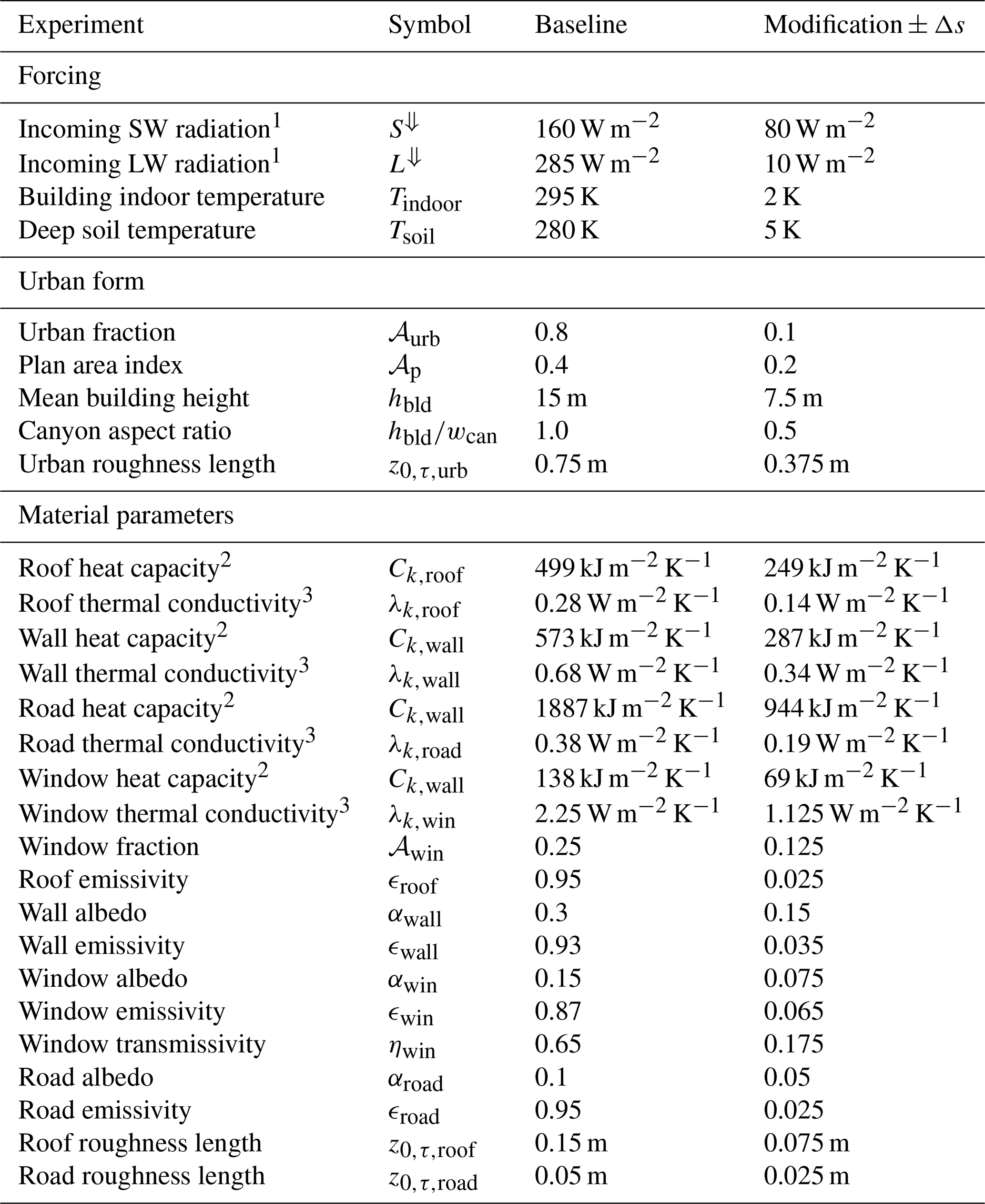
Some parameters have been aggregated for representation in the table: 1 diurnal average, 2 arithmetic sum aggregate over all material layers in the table, or 3 inverse of a harmonic sum aggregate over all material layers in the table.
Table 4Sensitivity tests for internal SLUrb parameterisations.
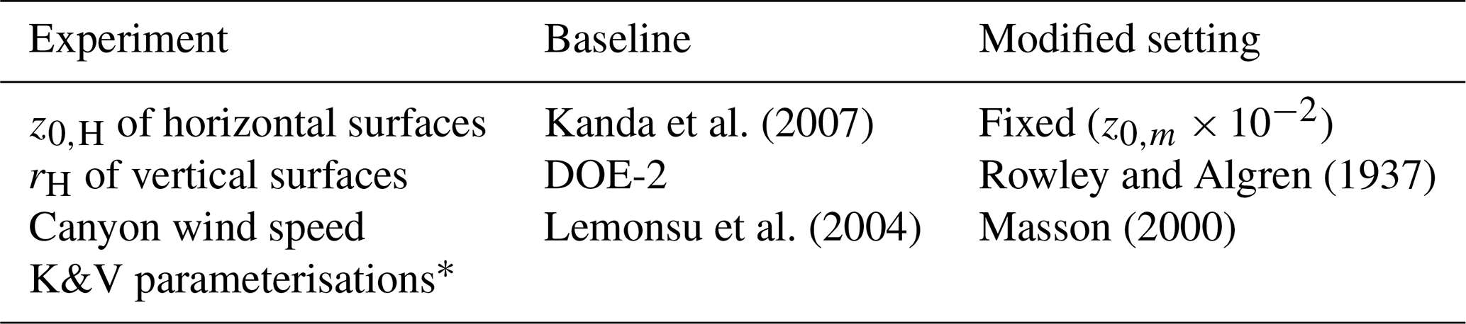
* Both the rH of vertical surfaces and the canyon wind speed are parameterised after Krayenhoff and Voogt (2007).
A simulation domain with and Nz=128 grid points and a uniform grid resolution of Δi=16 m, corresponding to a domain size of m3 in physical units, was used for all the simulations. The simulations were set up in LES mode with Boussinesq-approximated governing equations, a fifth-order upwind advection scheme after Wicker and Skamarock (2002), an iterative multigrid pressure solver (e.g. Hackbusch, 1985), a 1.5th-order subgrid-scale turbulence model after Deardorff (1980), and a third-order low-storage Runge–Kutta time-stepping scheme with a variable time step constrained by the Courant–Friedrichs–Lewy (CFL) condition (Williamson, 1980). A sponge layer was applied over the boundary layer (sin 2-damping with a factor of s−1 applied above 1536 m). The Coriolis frequency was set to s−1, corresponding to a latitude of 50° N.
To avoid the accumulation of effects from urban forcing, which would arise if periodic boundary conditions would be applied, a hybrid approach with a precursor run was utilised. With this approach, a precursor run with periodic boundary conditions was used to produce turbulent inflow data for the main experiment simulations. The precursor was initialised with typical springtime clear-sky conditions for Central Europe, as derived from the ERA5 global reanalysis (Hersbach et al., 2020). Furthermore, diurnal profiles of incoming shortwave and longwave radiative fluxes were computed from the ERA5-Land data that were used as external (prescribed) radiative forcing in both precursor and main simulations. A surface representing patches of vegetation following typical Central European vegetation typology was set up, with LSM used as the sole surface model. A more detailed description of the precursor setup is given in Appendix B.
The precursor was run for a total of 49 h, with the initialisation time set to 03:00 LST (local solar time). For convenience, the simulation time was defined to match the apparent solar time, aligning the maximum solar zenith angle to 12:00 LST. The turbulent inflow data were saved over a (y, z) cross section every time step of the last 25 h of the precursor, providing turbulent inflow for 1 h of flow spinup followed by a full 24 h diurnal cycle, from 04:00 to 04:00 LST the following day, for the main simulations. The resulting vertical and diurnal profiles of the mean wind speed, wind direction, potential temperature, relative humidity, and incident radiative fluxes, representing the overall forcing for the main simulations, are given in Fig. 2.
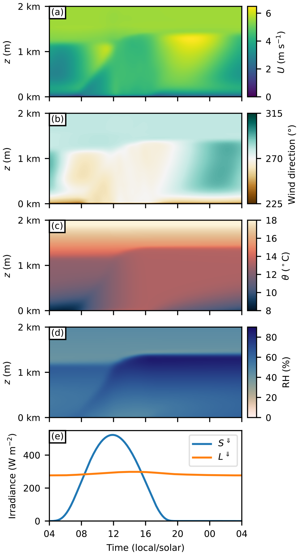
Figure 2Vertical profiles of the baseline forcing (a–d) as produced by the precursor run, and the applied diurnal profiles of shortwave and longwave incoming radiative fluxes at the surface (e) as computed from the ERA5 data. Together, the plots (a)–(e) represent the overall atmospheric forcing used in the main simulations.
The high-temporal-resolution cross-section data from the precursor run were imposed as a Dirichlet boundary condition in the main simulations, with an open boundary condition satisfying the Sommerfeld radiation condition and mass flow conservation used at the outflow boundary (Orlanski, 1976). Periodic boundary conditions were used for the (x, z) boundaries. For the surface, an urban area with an extent of 1536×1536 m2 was embedded, with a 2368 m and 192 m downwind distance from the inflow and outflow boundaries, respectively (Fig. 3). The vegetation type was set to short grass within the urban area, with the precursor surface reused elsewhere.
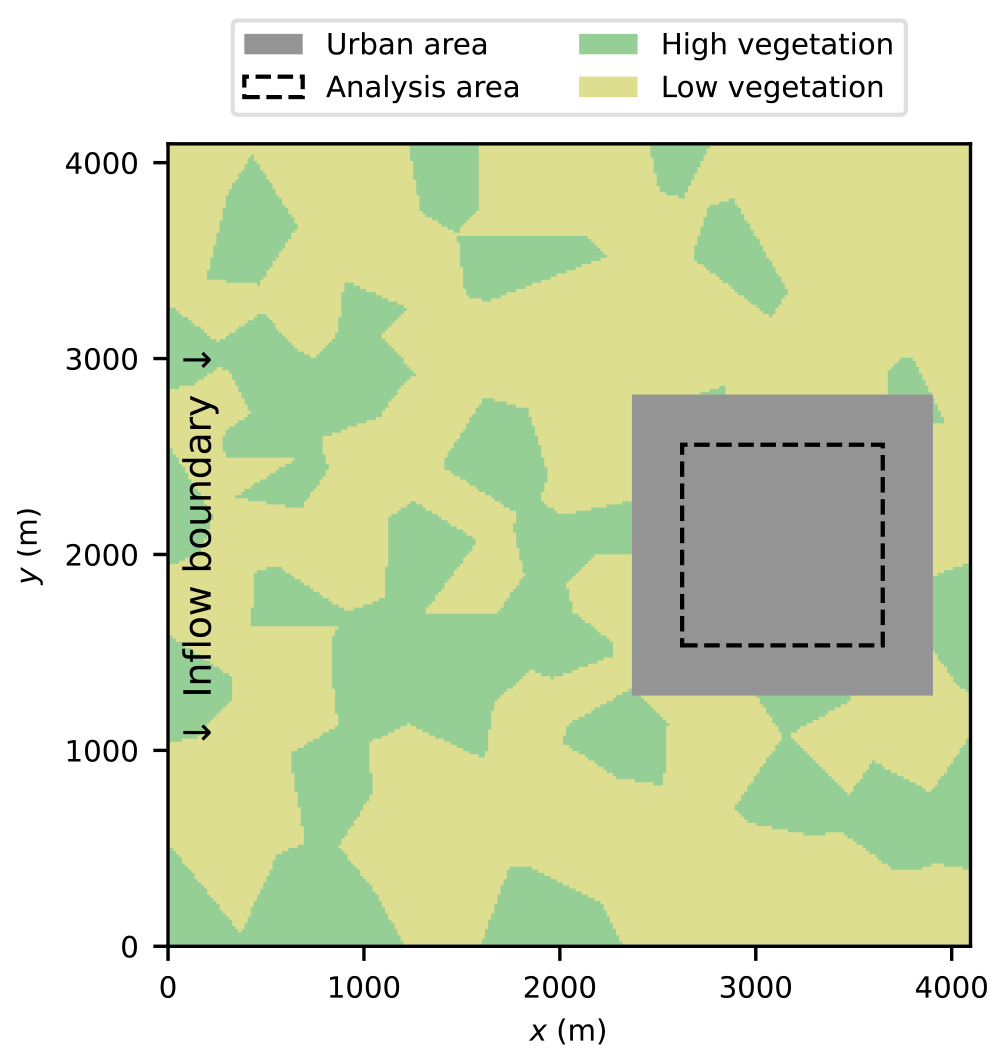
Figure 3Domain configuration for the sensitivity tests, representing a homogeneous target urban area embedded in a domain of mixed vegetation patches. The vegetation cover is simplified into two categories for the purpose of clarity, while the vegetation cover used in the simulations follows that used in the precursor (see Appendix B).
3.2 Analysis
The sensitivity of the modelling results relative to the model parameters and forcing variables was analysed against seven response variables. The selected response variables are sensible heat flux H, latent heat flux LE, ratio of sensible heat flux to net radiation , 2 m air temperature T2 m, area-weighted total urban surface temperature TC, canyon relative humidity RHcan, and total friction velocity u*. Total surface fluxes and friction velocity were used in the analysis, including both the urban contribution (SLUrb) and land surface contribution (LSM). Following a similar approach to that in SURFEX, 2 m air temperature T2 m was computed as a weighted average of the street canyon air temperature from SLUrb and the 2 m air temperature calculated using exponential interpolation by LSM for vegetation. All target variables were computed as an average over a rectangular area within the target urban area as presented in Fig. 3. The selection of the response variables was based on the consideration of SLUrb's intended use as an urban representation, especially used with relatively coarse grid spacings, where the total surface forcing and quantities describing the overall conditions within the urban canopy are of primary interest. To present the results in a concise and comparable form, they are reported using the response rate around the baseline based on the central difference:
where Y+ and Y− are the values of the response variable with the positive and negative modifications, respectively, X+ and X− are the modified values of the independent variable, and Xbase is the baseline value of the independent variable. Furthermore, we used a scaling factor of 𝒞s=0.1 to represent responses for a 10 % modification around the baseline for the given parameter or forcing variable. For the parameterisation tests, where the applied modifications in the baseline case are not numerical, such factors cannot be computed, and the results are reported as absolute differences relative to the baseline values.
It should be noted that in reality, at least for some parameters or forcing variables, the responses can be non-linear in nature, meaning that RR has a dependency on the selection of a baseline. Furthermore, a 10 % change in one parameter might be relatively small compared to its typical variation in the real world, whereas for another parameter, it might represent its whole physically realistic range. As an example, a 10 % difference in building indoor temperature corresponds to a difference of almost 30 K in absolute terms, which is far beyond the range of typical variability in the given variable. However, for incoming shortwave radiation, the corresponding absolute difference would be on the order of tens of W m−2 (diurnal average), which is well within typical variability of the variable. Thus, the response rates should be analysed in context and are used here only to provide a single figure for each of the tested forcing variables and model parameters. Thus, RR should be considered purely as a way to report the sensitivity with a single figure instead of a figure that would be truly comparable across the response and explanatory variables. Furthermore, they can be conveniently used to estimate the impact of uncertainty in an input if the range of the uncertainty is known.
The model sensitivity was analysed for both daytime and nighttime. The aggregation period for daytime values was defined as 12:00-16:00 LST, with nighttime values aggregated over 00:00–04:00 LST of the following night. The data were sampled from every time step for aggregation.
3.3 Results and discussion
As an overall reference of the model's diurnal behaviour, diurnal profiles of the target variables from the experiments with three different urban fractions are presented in Fig. 4. The largest differences are in daytime for fluxes and in nighttime for surface temperatures. Increasing the urban fraction increases H and lowers LE. Similarly, the 2 m air temperature increases slightly with the urban fraction over the diurnal period, whereas for TC, the effect is visible only during nighttime. For RHcan, the effect is relatively small. u* increases with the urban fraction as well, especially in daytime.
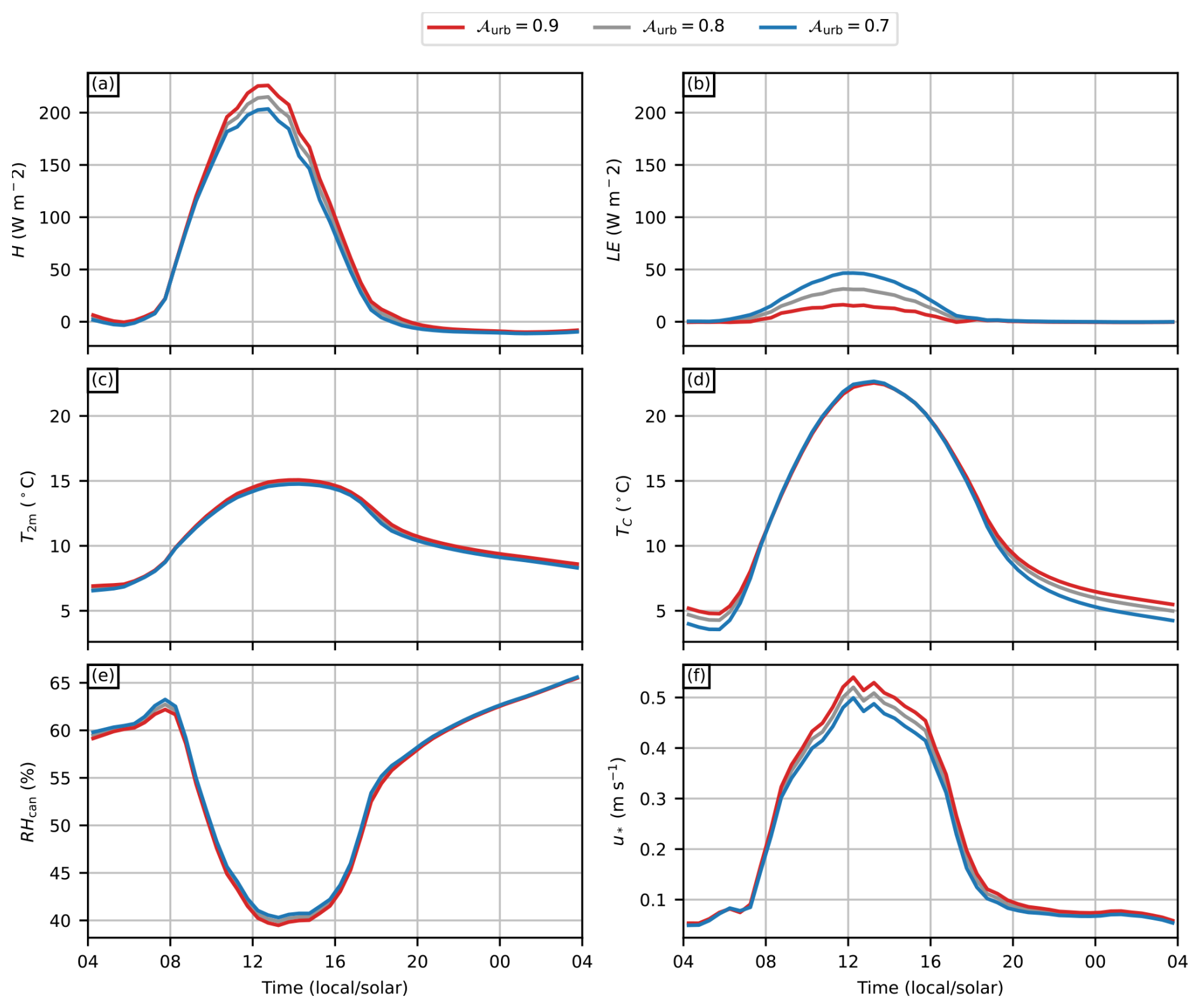
Figure 4Diurnal cycles of the sensitivity test target variables (a) sensible heat flux H, (b) latent heat flux LE, (c) 2 m air temperature T2 m, (d) area-weighted total urban surface temperature TC, (e) canyon relative humidity RHcan, and (f) total friction velocity u*, presented for three different urban fractions 𝒜urb.
The effect on heat fluxes is as expected: LE decreases with decreasing vegetation cover, and H represents higher partition of the total heat flux. The decrease in LE is slightly higher than the increase in H, which is explained by the higher storage flux of urban surfaces compared to vegetated surfaces. The relatively small effect on T2 m can be explained by the relatively small size of our target urban area, which means the upwind fetch over the urban area is, on average, very short, limiting the accumulation of urban heat. As TC by definition includes only artificial surfaces, there is no direct dependency on 𝒜urb, and hence the sensitivity to it is not very strong either. However, in the nighttime, TC is increased due to a small heat island effect and also due to slightly enhanced mechanical near-surface mixing.
As urban areas in our setup have higher roughness lengths than the vegetated surfaces, the enhancement of u* is expected; however, the effect and the magnitude of u* in all cases are relatively small during nighttime. It is worth noting that the coarse grid resolution used in the sensitivity tests might lead to an underestimation of the surface layer mixing in nighttime, leading to the underestimation of u* as well. The resolution sensitivity, however, is not analysed as a part of these sensitivity tests but as a part of the model comparison (see Sect. 4).
Table 5 presents the response rates RR for a set of target variables, as computed from the experiments with forcing-related variables. For H, the highest RR of 23.60 W m−2 is obtained for a 10 % variation in daily mean incoming shortwave radiation, followed by building indoor temperature and incoming longwave radiation. Deep soil temperature has an order of magnitude lower RR. For LE, the order of incoming longwave radiation and building indoor temperature is reversed, and the order of magnitudes of RR are 2 to 3 times lower than for H. Building indoor temperature has the highest RR for T2 m, and TC has the highest absolute (albeit negative) RR for RHcan. The radiative fluxes have the highest RR for u*, which follows from its strong dependency on surface stability.
Table 5Sensitivity of the target variables on forcing-related variables. The reported values are relative response rates RR scaled to a 10 % increment in the given parameter around the baseline. The target variables are sensible heat flux H (W m−2), latent heat flux LE (W m−2), ratio of sensible heat flux to net radiation (p.p.), 2 m air temperature T2 m, area-weighted urban surface temperature TC (K), canyon relative humidity RHcan (p.p.), and total friction velocity u* (m s−1).
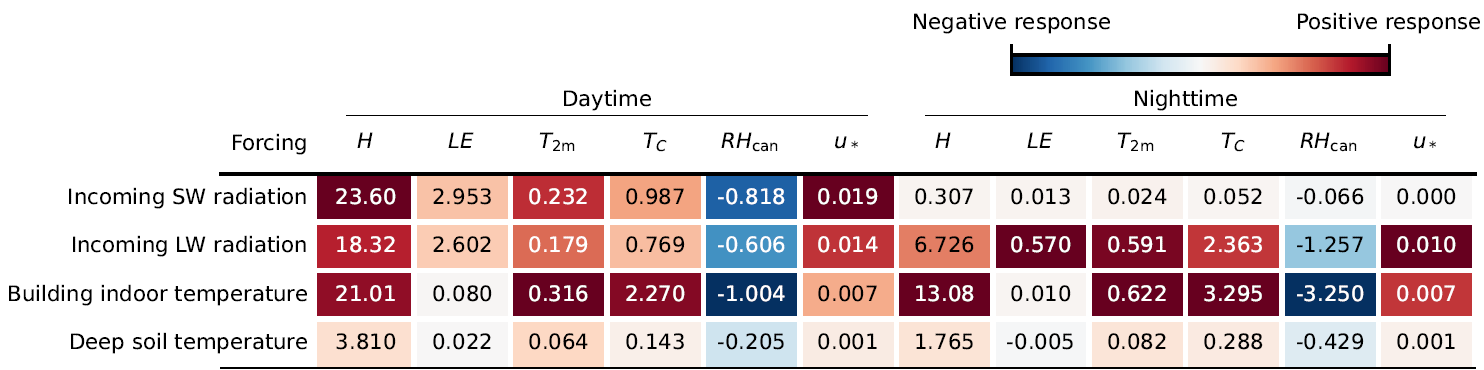
For nighttime values, the sensitivity to daily mean incoming shortwave radiation decreases significantly, with building indoor temperature and incoming longwave radiation having the highest RR. For LE, RR is lower than for H for all tested forcing variables. Building indoor temperature has the highest RR for T2 m and TC and the highest absolute RR for RHcan. For u*, incoming longwave radiation has the highest RR.
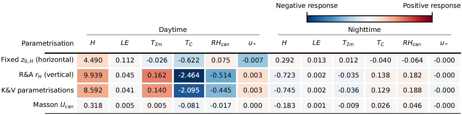
Table 6Sensitivity of the target variables to the used internal parameterisations in SLUrb. The reported figures are absolute differences relative to the baseline. The target variables are sensible heat flux H (W m−2), latent heat flux LE (W m−2), ratio of sensible heat flux to net radiation (p.p.), 2 m air temperature T2 m, area-weighted urban surface temperature TC (K), canyon relative humidity RHcan (p.p.), and total friction velocity u* (m s−1). The colour scale is the same as that in Table 5.
Overall, the responses to the changes in forcing are relatively straightforward to explain. In daytime, the shortwave radiation contributes the most significant inflow of energy to the system, followed by longwave radiation. However, RR of building indoor temperature is higher, as the scaling to a 10 % change in explanatory variables corresponds to an extremely high range of building indoor temperatures. Thus, in a realistic setting, the building indoor temperature has much lower importance than the aforementioned incoming radiative fluxes. However, for longer simulation times, the temperature boundary conditions (building indoor temperature and deep soil temperature) are expected to become more important. Increased incoming radiative fluxes subsequently increase the surface heat fluxes, and with a high baseline urban fraction of 𝒜urb=0.8, the majority of this is partitioned into sensible heat. This in turn increases T2 m and lowers RHcan. Furthermore, an increase in both H and LE increases the overall surface buoyancy flux, enhancing mixing and increasing u*. In nighttime, the sensitivity to the incoming shortwave radiation is decreased due to its diurnal profile, and only some residual effect remains through increased heat storage.
The sensitivity to the selection of internal parameterisation options implemented in SLUrb is presented in Table 6. Interestingly, the default set of parameterisations affecting both horizontal and vertical surfaces yields lower sensible heat fluxes for both day and night than their alternatives. However, the magnitude of the difference is not particularly high compared to the diurnal average. The effect on LE is negligible, which is mainly due to a representative clear-sky day used as a baseline. With precipitation or stronger dewfall events, for example, the sensitivities would probably be higher. As expected, higher H leads to lower surface temperatures, as seen in TC. Overall, using the Masson (2000) parameterisation for Ucan instead of the default Lemonsu et al. (2004) results in negligible changes in all the target variables, but the effect might be more significant in different flow regimes.
Finally, RR values computed for the model parameters are presented in Table 7. Overall, the urban fraction has the highest absolute RR for almost all target variables, in both daytime and nighttime. The urban fraction is followed by the plan area fraction and, especially for daytime and u*, the urban roughness length. Increasing the plan area fraction increases the built surface area directly exposed to the atmosphere, which explains its positive correlation with H as well as correlations of opposing signs of daytime and nighttime TC.
Table 7Sensitivity of the target variables to the model parameters. The reported figures are the response rates RR scaled to a 10 % increment in the given parameter around the baseline. The target variables are sensible heat flux H (W m−2), latent heat flux LE (W m−2), ratio of sensible heat flux to net radiation (p.p.), 2 m air temperature T2 m, area-weighted urban surface temperature TC (K), canyon relative humidity RHcan (p.p.), and total friction velocity u* (m s−1). The colour scale is the same as that in Table 5.
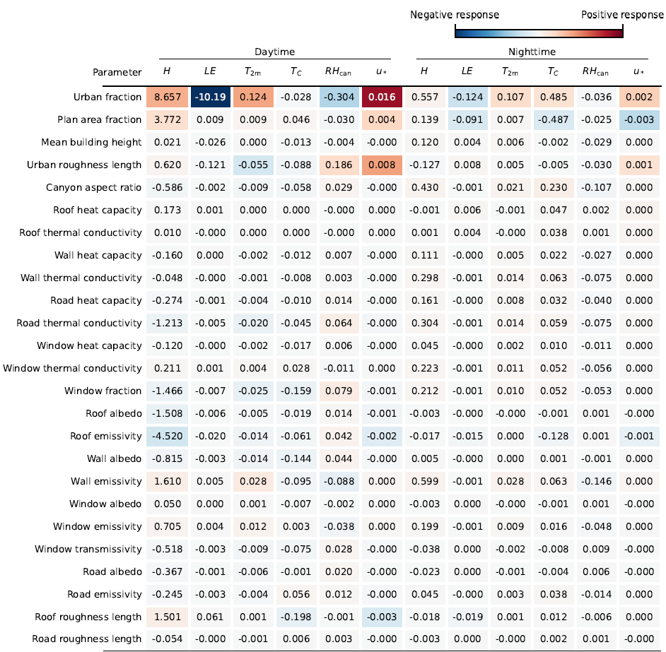
Of the other morphological parameters, increasing the canyon aspect ratio slightly decreases fluxes but increases nighttime temperatures, which can be explained by the enhanced longwave trapping within the street canyon. While the mean building height has relatively minimal direct effect in the model, it is worth noting that the semi-empirical parameterisations often used to determine the urban roughness length from surface data typically have a strong dependency on it. This also highlights that, while in these sensitivity tests the parameters are changed one at a time, in reality, there are strong interdependencies among them.
The model is moderately sensitive to the radiative parameters of roofs, walls, windows, and roads and relatively insensitive to their thermal parameters. As roofs are not influenced by radiative trapping, the model is more sensitive to the roof radiative parameters than to those of the canyon surfaces. The sensitivity to emissivity is generally higher; however, their typical range is small (0.85–0.97) when compared, for example, to albedos (0.05–0.90) of typical urban surface materials (Oke et al., 2017).
The observed model sensitivity is generally well in agreement in terms of both the direction of change and the magnitude with those reported in TEB evaluation studies (e.g. Masson et al., 2002; Lemonsu et al., 2013), although not all target variables and parameters covered here are represented in these studies. The sensitivity to the internal parameterisations is not extensively studied in prior literature, and in the case of SLUrb, a more detailed evaluation, especially against real-world measurements, would be needed to better understand their performance and limitations.
The applicability of SLUrb in representing urban surfaces across various grid resolutions was assessed through a model comparison experiment. The focus was to evaluate SLUrb's fitness for its purpose within the PALM model system, which is to produce surface forcing and neighbourhood-scale bulk meteorological conditions comparable to the high-resolution resolved canopy at lower than building-resolving resolutions.
In the model comparison experiment, SLUrb was compared against PALM's building-resolving approach, which explicitly resolves the turbulent transport processes and three-dimensional radiation interactions within the urban canopy. In contrast to an evaluation against, e.g., real-world measurements or other model systems, this approach limits the effect from the uncertainties arising from the rest of the model system, its schemes, numerics, and boundary conditions. By comparing against different surface representations within the same modelling system, observed differences could be directly linked to the differences in the surface representation.
The primary goal was to evaluate the resolution sensitivity of the resulting surface forcing from both models. The comparison focused on scenarios where resolving individual buildings is impractical but a reliable representation of urban–atmosphere interactions and a broad characterisation of atmospheric conditions within the urban canopy are still required.
4.1 Experiment setup
Single model runs with both the resolved urban canopy and SLUrb were performed using a one-way self-nesting to embed multiple domains with distinct grid resolutions into a single simulation. The root domain was set up similarly to the sensitivity tests (see Sect. 3), utilising the same turbulent inflow method used in the sensitivity tests for forcing, with a (y, z) inflow plane recorded from the precursor run used as a Dirichlet boundary condition. The setup ensures that the inflow boundary condition as well as the total mass flow remain the same in both simulations regardless of changes in surface friction. The same external incident radiation (before radiative interactions) as for the precursor was used in the model comparison as well. An overview of the forcing over the full diurnal cycle is presented in Fig. 2.
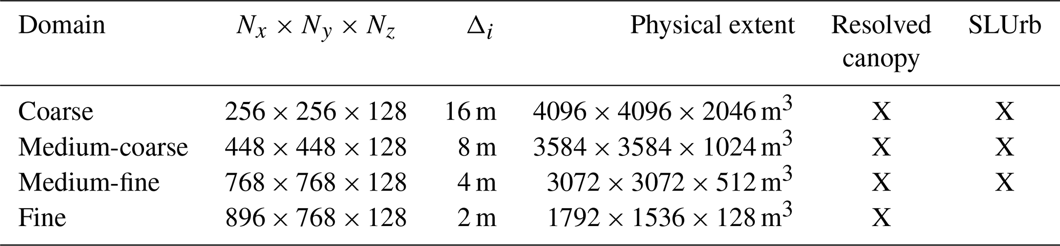
With the resolved urban canopy, four domains with grid resolutions of 16, 8, 4, and 2 m were used. The highest-resolution domain was omitted from the simulation with SLUrb, as coupling an urban surface with high roughness length with such a high grid resolution is not technically justifiable. An overview of the domains, together with their extents in grid points and physical dimensions, is given in Table 8. This approach had the benefit of allowing a gradual refinement of the grid resolution from the Δi=16 m inflow boundary for the inner domains, avoiding the need to run separate and computationally expensive setups for each resolution.
Table 8The nested domain setup as used in the model comparison. The first four columns are the domain name, domain size in grid points, grid resolution (uniform), and physical extent of the domain. The last two columns signify in which of the simulations the given domain is included.
The same numerical setup as in the sensitivity tests was used for the atmospheric model in all of the domains (root and nests), meaning the usage of the LES mode with the Boussinesq approximation, a fifth-order upwind advection scheme (Wicker and Skamarock, 2002), an iterative multigrid pressure solver (e.g. Hackbusch, 1985), a 1.5th-order subgrid-scale turbulence model (Deardorff, 1980), and a third-order low-storage Runge–Kutta time-stepping scheme with a variable time step constrained by the Courant–Friedrichs–Lewy (CFL) condition (Williamson, 1980; Baldauf, 2008), with a sponge layer applied in the root domain over the boundary layer (sin 2-damping with a factor of s−1 applied above 1536 m). The Coriolis frequency was again set to s−1, corresponding to a latitude of 50° N.
4.1.1 Resolved urban canopy surface setup
To extend the coverage of the comparison into more than one class of urban form, the target urban area was subdivided into a mosaic of 36 patches of size 256×256 m2 representing dense midrise and open midrise urban areas (LCZs 2 and 5, respectively; see Fig. 5).
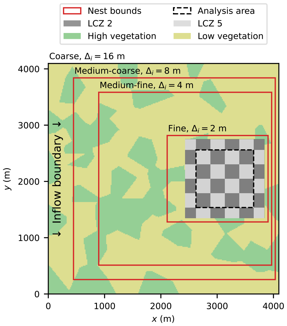
Figure 5A schematic overview of the modelling approach for the model comparison, representing a mosaic of urban patches surrounded by mixed vegetation patches. The vegetation cover is simplified into two categories for the purpose of clarity, while the vegetation cover used in the simulations follows that used in the precursor (see Appendix B for further details).
A generated three-dimensional medium-rise urban form corresponding to the prescribed LCZ mosaic was used for surface definition in all of the domains of the resolved urban canopy simulation. The surface definition was initially generated at an original resolution of 2 m and was subsequently downsampled for use in the coarser-resolution domains. Using PALM's resolved urban canopy approach, building surface energy balances were modelled with USM, vegetation and pavements by LSM, and radiative interactions of all the surfaces with RTM. The default configuration of the RTM was used, with three reflection steps and 80 azimuthal and 40 elevation angles used for angular discretisation. A very short fixed radiation time step (2 s) was applied to minimise potential errors from temporal discretisation.
The final urban forms in the simulation domains after downsampling and PALM's internal topography filtering process, which iteratively fills cavities resolved to less than 10 grid cells, are presented in Fig. 6. The figure highlights the effect of resolution reduction on, e.g., the building height variation, street canyon network, total three-dimensional urban surface area, and variability in the urban form in general.
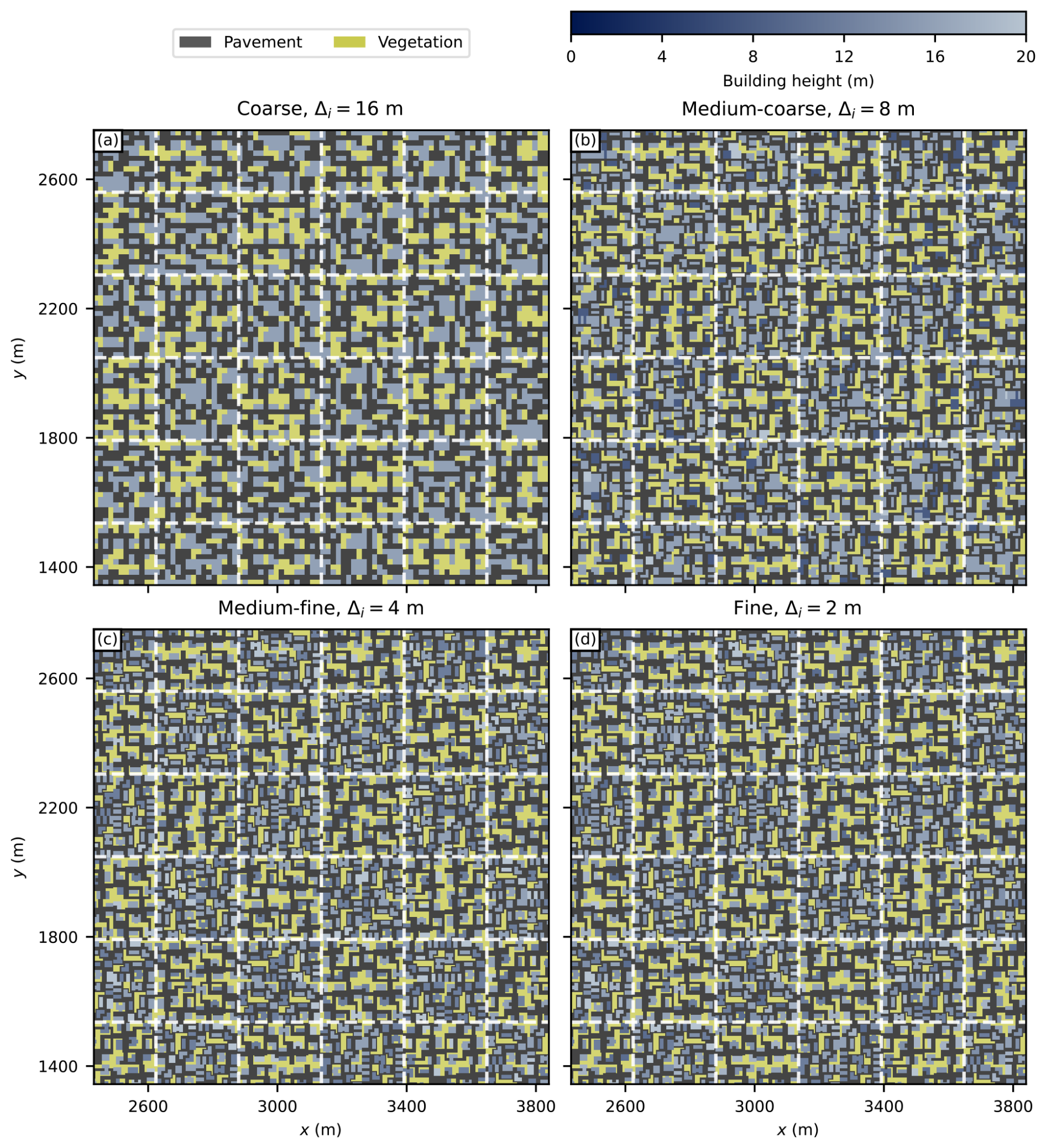
Figure 6Surface representation of the resolved urban canopies after downsampling and filtering for the four grid resolutions. The white dashed grid lines represent the limits of the LCZ mosaic (see the chequerboard pattern in Fig. 5), with LCZ 2 tiles having a higher packing density of buildings). The x and y axes are defined as distances to the root domain (bottom-left) origin.
4.1.2 SLUrb surface setup
The two-dimensional surface inputs of urban morphological parameters (𝒜p, 𝒜urb, hbld, , and ) needed for the SLUrb model were estimated from the original 2 m resolution urban form. 𝒜p, 𝒜urb, and hbld were directly computed from the three-dimensional surface. The vegetation was modelled with LSM using the mixed-tile mosaic approach, with vegetation coverage being exactly the same as in the resolved urban canopy simulations. The street canyon aspect ratio was estimated from the surface using the relation
where Rfac,p is the ratio of the facade (vertical surface) area to total plan area, as computed directly from the three-dimensional surface. To estimate , a parameterisation by Macdonald et al. (1998) for staggered obstacle arrays was used. The resulting values for both LCZs are given in Table 9. It is worth noting that the Macdonald et al. (1998) parameterisation predicts lower for LCZ 5 than for LCZ 2 despite the lower urban fraction due to a high packing density of buildings in LCZ 2.
Table 9Morphological parameters for local climate zones 2 and 5 as derived from the three-dimensional urban form used in the resolved urban canopy approach.
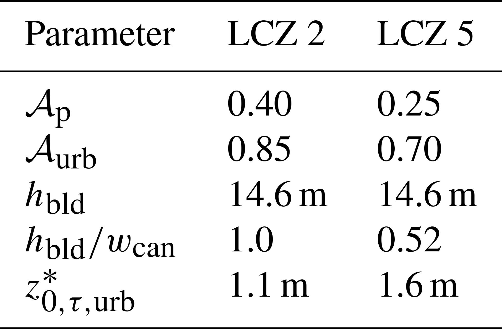
* Estimated using the Macdonald et al. (1998) method for staggered obstacle arrays.
4.1.3 Surface parameters and initialisation
To ensure the resolved urban canopy simulation and the SLUrb setups are as comparable as possible, thermal and radiative surface and subsurface parameters in both simulations were manually set to identical values as those used in the baseline case of the sensitivity tests (see Sect. 3). A complete list of these parameters is given in Appendix C.
In order to make the initial conditions of the models comparable, it was essential to consider the differences in model spinup approaches. With the resolved canopy approach, PALM's surface model spinup scheme computes surface and subsurface energy balances using a reference diurnal temperature cycle imposed on the surface-adjacent grid cells while maintaining constant atmospheric variables such as wind speed and humidity. In contrast, SLUrb includes additional prognostic equations for street canyon air and local friction velocities during its spinup, extending beyond just energy balance computations.
To specifically compare the two modelling approaches with a focus on the two-way coupled atmospheric simulation, the surface model spinup was performed only with the SLUrb model. Thus, identical initial conditions as copied from the SLUrb simulation – including wall, roof, road, window, and soil layer temperatures, as well as soil humidity – could be used for the resolved urban canopy at the start of the atmospheric simulation.
4.2 Analysis
The main focus of the comparison was in the resulting atmospheric forcing from the urban surface as a whole. In the case of SLUrb, where the surface interaction is completely parameterised, the total forcing from urban form to the atmosphere is directly available as standard two-dimensional surface outputs. Sensible heat (H), latent heat, and friction velocity (u*) were selected for comparison, as they represent the total surface forcing relevant for atmospheric dynamics.
The direct surface fluxes as computed from the model surfaces of the resolved urban canopy are not directly comparable to those obtained with SLUrb and LSM, as the former represent the local surface interaction instead of the total exchange between the urban canopy and atmosphere above it. To derive comparable fluxes for the former case, the respective local flux was first integrated over the local three-dimensional surface, after which a term representing a change in heat stored in the air within the urban canopy itself could be obtained. Averaged over an area of interest, this can be written as
where 〈H〉 and 〈LE〉 represent the total heat fluxes between the urban canopy and the atmosphere above the roof height, H0 and LE0 are the local surface fluxes, (xs, ys, zs) are the coordinates of the three-dimensional surface, A signifies the total three-dimensional surface within the averaging area of interest with a top-down projected area of R, and V is the air volume confined within the averaging area and below the first model level above the highest roof level.
For the momentum flux, the local skin friction of the surfaces represents only a minor part of the total momentum sink, with pressure drag caused by the resolved obstacles, buildings in this case, being much more significant. On the other hand, unlike the case for heat, the changes in the momentum storage of the urban canopy air are negligible compared to the two aforementioned momentum forcing mechanisms. Thus, a representative friction velocity combining contributions from both local friction and pressure drag forces in both the x and y directions was computed for the resolved urban canopies as follows:
where
is the mean pressure drag force magnitude within the averaging area, is the local friction velocity, p* is the perturbation pressure, and p∞ is the domain-average perturbation pressure, which may be non-zero in PALM for nested domains with all-Neumann boundary conditions for p* (Hellsten et al., 2021). An indicator function χi has a value of 1 where there exists a surface facing the given direction i in the grid cell, −1 if there is a surface facing the opposite direction, and 0 elsewhere.
In addition to surface forcing, the street canyon air temperature Tcan and relative humidity RHcan were compared, as at least the overall meteorological conditions within the urban canopy are likely to be interesting in city-scale urban studies also at coarser 𝒪(10 m) resolutions. Following SLUrb's definition of these variables, they were computed for canyon mid-height in the case of resolved urban canopy as well.
4.3 Results and discussion
In Fig. 7, the diurnal cycles of the studied variables from both simulations with SLUrb and the resolved urban canopy, spatially averaged over the 16 inner urban patches (see Fig. 5), are presented. Overall, we can observe similar diurnal behaviour with both approaches at all studied resolutions, with H, LE, u*, and Tcan peaking at noon or afternoon, with RHcan mirroring the behaviour.
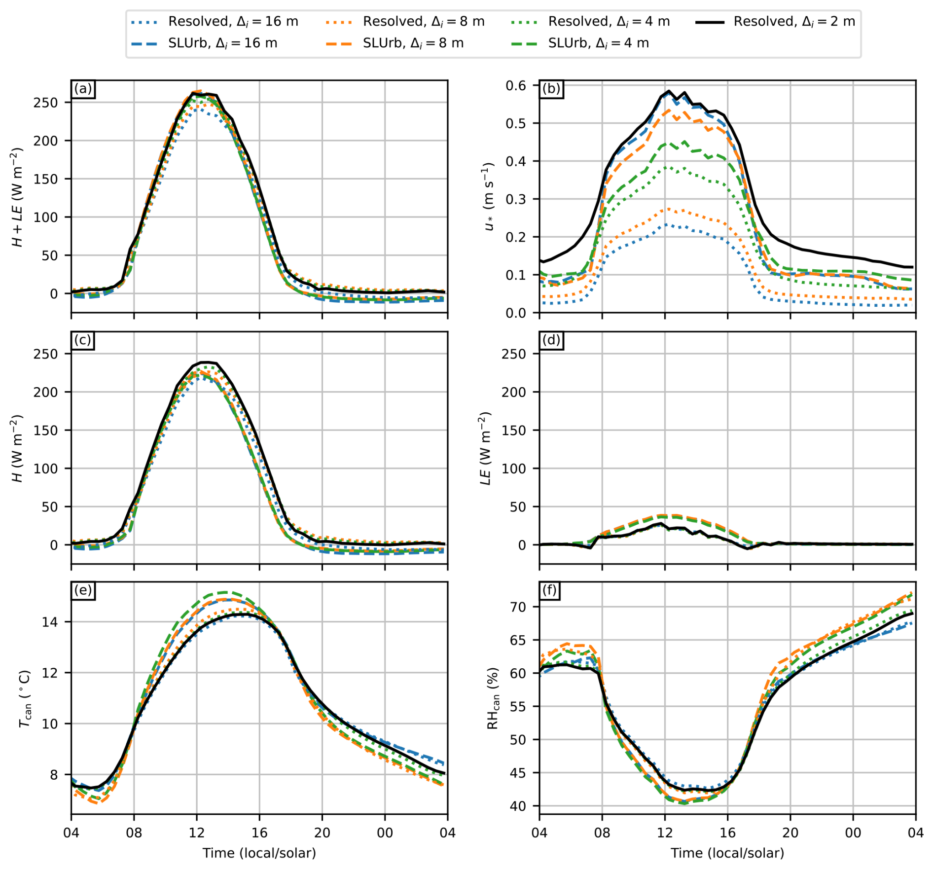
Figure 7Diurnal cycles of (a) total heat flux, (b) friction velocity, (c) sensible heat flux, (d) latent heat flux, (e) street canyon air temperature, and (f) relative humidity from both resolved urban canopy and SLUrb simulations. The diurnal cycles are spatially averaged over the 16 inner urban patches as illustrated in Fig. 5.
As surface thermal and radiative parameters as well as the radiative fluxes incident on the urban average are, on average, set to the exact same values in both simulations and with all resolutions, the main differences in total heat flux (H+LE) arise from differences in the internal heat transport and flux partitioning in the models. The flux is very similar in all cases especially during daytime, with the resolved urban canopies showing slightly more resolution sensitivity. With the resolved urban canopies, the total urban surface area as well as radiative interactions change with respect to the resolution, decreasing H with decreasing resolution. Towards and during nighttime, an increasing difference between SLUrb and resolved canopy simulations can be observed.
Partitioning the total heat flux into sensible and latent heat fluxes shows a more significant difference between the modelling approaches. Representing urban areas with SLUrb yields a slightly lower Bowen ratio than the resolved canopy approach. This is somewhat expected, as the initial version of SLUrb considers vegetation only through a surface tile mosaic approach together with LSM. Because in this approach the vegetation is not integrated within the urban canopy but rather considered using the mosaic approach, the vegetation receives more direct shortwave radiation than in the resolved urban canopies due to the absence of shading by buildings. As the model comparison setup represents clear-sky conditions with dry urban surfaces, latent heat is originated purely from the vegetated surfaces. Thus, the resulting lower Bowen ratio is inherent to the current technical implementation of mixed urban-vegetation tiles in SLUrb.
Out of all the variables, u* shows the highest resolution sensitivity for both approaches. The total u* with the resolved canopy approach decreases drastically with increasing grid spacing over the whole diurnal cycle (0.09 and 0.29 m s1 for the diurnal mean and 16 and 2 m grid spacings, respectively), whereas the dependency is the opposite, albeit smaller, for SLUrb in daytime and indefinite in nighttime. The surface friction as modelled with SLUrb at the coarsest resolution matches very closely the total u* of the resolved canopy, with the finest 2 m resolution in daytime (0.54 and 0.55 m s1, respectively), and is somewhat lower in nighttime (0.08 m s1 vs. 0.13 m s1).
By examining the surface definition in the resolved urban canopy simulation as a function of resolution (Fig. 6), we can observe a clear decrease in surface heterogeneity with higher grid spacings due to the downsampling and filtering operations. In addition to the loss of detail in the surface description itself, the modelling of turbulent transport processes is affected by the grid resolution, contributing a further increase in resolution sensitivity.
Although the model equations in SLUrb do not have any direct dependency on grid resolution, there is an indirect dependency that affects the results, especially for momentum flux in daytime. With high resolutions and rough surfaces, the assumptions of MOST, on which PALM's surface coupling relies, are violated. The limitations in using MOST to represent rough surfaces with fine grid spacings in LES has also been discussed in the literature in recent years (e.g. Harman and Finnigan, 2007, 2008; Basu and Lacser, 2017), and they generally affect PALM as well. Nevertheless, SLUrb compares closer to the 2 m resolved canopy simulation in terms of total momentum forcing than the simulations with the resolved canopy at lower resolutions.
Both SLUrb and resolved canopies yield lower total surface friction in nighttime than the reference resolved canopy with the 2 m resolution. The sensitivity with the resolved canopies can be explained using the same reasons as for daytime; meanwhile, with SLUrb, some of it can be attributed to the limitations of MOST with stable stratification. However, we can observe a drop in SLUrb-modelled friction velocity with the 16 and 8 m resolution domains but not with the 4 m domain. Such reversal in resolution dependency is not explained by the limitations in MOST as discussed above but rather may be related to inherent limitations in representing subgrid-scale momentum diffusion in stably stratified flows with coarser resolutions and with the default Deardorff 1.5th-order subgrid turbulence model, which lead to insufficient vertical transport of the momentum at subgrid scales. This and related issues are discussed in more detail in the works of, e.g., Gibbs and Fedorovich (2016), Dai et al. (2021), Gehrke et al. (2021), and Resler et al. (2024), where the first two of these suggest their own revised versions of the Deardorff model to mitigate the issue. However, Gehrke et al. (2021) reported that using the Dai et al. (2021) model did not improve the near-surface mixing in their case.
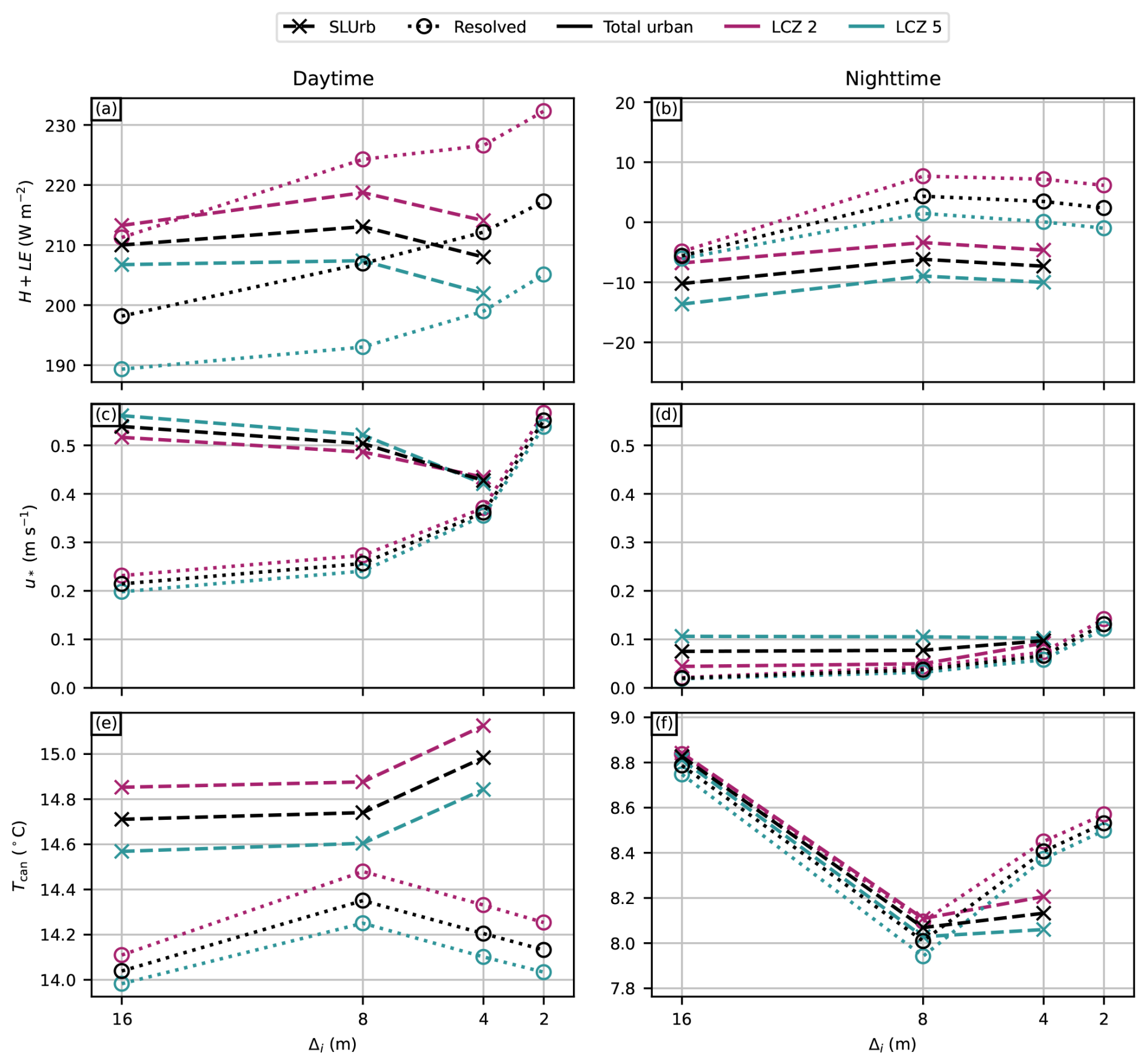
Figure 8Plots of (a, b) total surface heat flux, (c, d) friction velocity, and (e, d) street canyon air temperature for the total urban area and LCZs 2 and 5, presented as a function of grid spacing separately for daytime (a, c, e) and nighttime (b, d, f). Note the different ranges for the y axes for the daytime and nighttime panels.
It is worth noting that the applied boundary conditions can influence the overall magnitude of the u* resolution sensitivity. In our setup, the total mass flow rate of the domain is conserved. This, combined with the fixed Dirichlet inflow boundary condition at the inflow, means that the pressure gradient force (on average over the whole domain) must compensate for any added surface friction. If a constant pressure gradient would be applied as a momentum forcing instead of the turbulent inflow, the added friction could at least, in theory, decrease the total mass flow through the domain. This could, in turn, decrease the near-surface wind speeds, limiting the u* values in the case of high friction. Therefore, with a fixed pressure gradient instead of a fixed inflow, the resolution sensitivity of u* could be smaller.
The diurnal amplitude of Tcan is approximately 7 °C with the resolved canopy and 8 °C with SLUrb, and the behaviour overall is in good agreement. The temperatures within the resolved canopy reach the maximum slightly later compared to SLUrb, indicating a slightly stronger overall hysteresis of the urban surface. However, the differences are rather small. At least part of the difference may be again explained by the approach used with SLUrb to represent mixed urban-vegetation surface tiles, which also leads to the lower Bowen ratio of surface fluxes. As the air temperature is a dominant component determining relative humidity in general, the overall source of humidity is small due to the relatively high u, as expected.
Figure 8 provides another view of the resolution sensitivity of the total heat flux, friction velocity, and street canyon air temperature, averaged separately for daytime and nighttime and for the two LCZs. The internal order of LCZs 2 and 5 is the same for both the resolved canopy approach and SLUrb for H+LE and Tcan and reversed for u*. The resolution dependency itself does not seem to depend much on LCZ, except with SLUrb and u*, where the limitations of MOST representing rough surfaces with finer grid spacings discussed earlier likely contribute to the loss of distinction between the LCZs, particularly with the 4 m grid spacing.
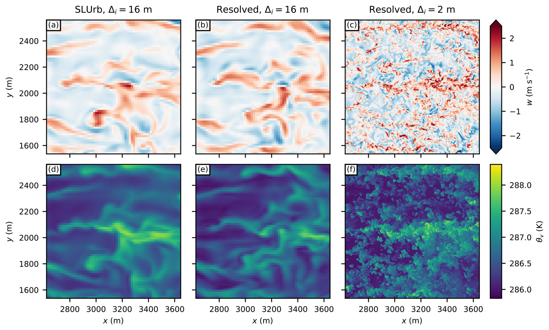
Figure 9Instantaneous (x, y) cross sections of model vertical velocity w (a–c) and virtual potential temperature θv (d–f) over the analysis area from a model level closest to z=42 m at 12:00 LST (solar noon). The cross sections are presented for SLUrb at 16 m grid resolutions (a, d) and for the resolved urban canopy at 16 and 2 m grid resolutions (b, e and c, f, respectively).
The parameterisation following Macdonald et al. (1998) used to estimate for the LCZs predicted a higher value for LCZ 5 than for LCZ 2 due to the increased plan area fraction. As SLUrb relies on this input parameter when determining the relative roughnesses of urban areas, it directly follows that it models higher u* for LCZ 5. Thus, SLUrb's capability to capture the difference in urban surface roughnesses can be only as good as the parameterisation used for , which is something potential model users should consider when preparing the simulations. The difference in u* in the resolved canopy simulation between the LCZs is very minor compared to the resolution sensitivity and almost vanishes in the highest-resolution domain.
Finally, as a qualitative reference of spatial flow structures produced by the surface forcing, Fig. 9 presents instantaneous (x, y) cross sections of the model vertical velocity w and virtual potential temperature θv over the analysis at one model height (the closest to z=42 m) at 12:00 LST (solar noon). Both the SLUrb and resolved urban canopy approaches produce stream-wise elongated convective structures at 16 m, which match the spatial patterns produced with the resolved urban canopy at 2 m resolution.
The first release of SLUrb, despite implementing most of the functionalities typically found in single-layer urban canopy models along with some additional ones, is still missing some features often found in more mature surface models. The shortcomings include, e.g., the lack of representation for in-canyon vegetation and snow cover. One of the main findings of the first phase of the Urban-PLUMBER model intercomparison project was that the inclusion of vegetation in canyon models generally improved the model performance in terms of minimising errors in modelled fluxes compared to the benchmark (Lipson et al., 2024). Although the current implementation is capable of representing mixed urban-vegetation tiles by the aggregation of fluxes from SLUrb and LSM, the vegetation modelled by LSM is not affected by building shading or other radiative processes. In the long term, additional vegetation tiles as modelled by LSM could be added within the canyon to model the full vegetation and hydrological processes. However, many of LSM's aspects are hard-coded for representing fixed, non-fractional surface tiles of the resolved PALM topography. Therefore, a technical overhaul of LSM would be needed in order to allow SLUrb, or any other future model component, to use it for representing internal vegetation surfaces in the way that, e.g., ISBA is utilised in the SURFEX implementation of TEB. Such overhaul would require its own validation and performance testing. An intermediate, much simpler solution in the current development roadmap is to implement a proxy model for canyon vegetation similar to the one in WRF-TEB (Meyer et al., 2020). Nevertheless, implementing a scheme for canyon vegetation would not replace the current tile approach with SLUrb and LSM, as the need to represent urban surfaces mixed with larger vegetated areas (e.g. parks and forests) or water bodies would remain. Implementation of snow cover for SLUrb is currently on hold until such implementation is made for LSM in order to ensure consistency of the models.
The current implementation of SLUrb uses user-defined indoor air temperature as a boundary condition rather than computing it dynamically using an indoor air model that would account for heating, ventilation, and air conditioning (HVAC). Although PALM already includes a coupled HVAC model (Pfafferott et al., 2021), it is targeted towards grid-resolved buildings and cannot be simply reformulated for parameterised urban canopies as assumed in SLUrb. Our sensitivity tests suggest that indoor temperatures have a relatively small impact on tile-aggregated fluxes and temperatures on timescales of 1 d. However, for investigating heat-wave situations with longer simulation periods of 1 week, Maronga et al. (2022) showed that HVAC contributions can become significant in terms of air temperatures. Hence, we encourage future studies to revisit the HVAC model in PALM and introduce a coupling with SLUrb, which would be a valuable addition, especially for simulating heat-wave scenarios.
As a new model component, SLUrb still lacks integration with some of the other PALM modules, such as surface emissions for aerosol and chemistry modules, limiting the applicability for air quality and dispersion studies. Integrating SLUrb further with the model system is in the development roadmap for future PALM releases. While the coupling with the atmospheric model of PALM in Reynolds-averaged Navier–Stokes (RANS) mode is, in principle, possible, it has not been tested beyond small initial tests. In the near future, one aim is to allow running SLUrb on GPUs by further parallelising the internal loops using OpenACC and OpenMP.
SLUrb models the aerodynamic resistances in the vertical direction using the framework of MOST. The limitations of MOST are widely acknowledged in the literature, especially in the case of strong near-surface anisotropy of turbulence due to stable stratification or a complex terrain (e.g. Foken, 2006; Stiperski and Calaf, 2023), as highlighted for the former case in the model comparison results for nighttime. Based on the model comparison results, the model may have difficulties in accurately representing near-surface mechanical mixing with finer grid resolutions, which may be due to the lack of a roughness sublayer correction. Implementing such correction is an aspect that could merit more investigation and experimentation for future model versions. However, to maintain consistency of PALM's surface representation, such adjustment should be implemented at the same time for, e.g., high vegetation modelled by LSM. As there is no clear consensus on the universal form of such correction nor extensive empirical evidence on the performance of the proposed ones, implementing such change in LSM or PALM surfaces in general would require careful evaluation. Thus, improving the PALM model system in this regard was deemed out of the scope of the work presented here.
As SLUrb is a single-layer urban canopy model based on the infinite two-dimensional canyon assumption, it is out of its scope to represent conditions within the urban canopy in great detail. Thus, SLUrb is not capable of giving detailed information from exact spots within the urban canopy, e.g. the air temperature and wind speed in a particular street corner within a real urban area, and will not replace the need of running simulations with resolved urban canopies at high resolution for studies needing the detailed representation of canopy processes.
At the current stage, SLUrb should be considered an experimental model, meaning it has not yet undergone comprehensive testing and evaluation against a wide range of empirical data across diverse scenarios. To complement the technical evaluation presented in the paper, it would be beneficial to compare SLUrb's outputs against real-world urban observations, such as eddy covariance flux measurements, satellite surface temperatures, and spatiotemporal distributions of urban heat as measured by dense observational networks. As with any experimental model, users should approach its results with an appropriate level of caution. Before drawing conclusions based on the model's results or using it in production applications, users are strongly advised to assess its performance in the context of their specific use cases.
Gathering input data and pre-processing that data to exactly the form that a model uses as input can be a tedious task. Currently, there exists no generator for the SLUrb input driver, making its creation a manual process for the users. Although creating a universal generator that would process any form of raw urban surface data from start to finish would be technically unfeasible, a generator working with a pre-defined set of surface maps is on the roadmap for future releases.
Finally, potential users should note that there is a known bug with SLUrb restart routines when using MPI I/O for restarts, which was noticed only after the release. With the current release, the issue can be mitigated either by using a serial I/O method for the restarts or by applying a patch included in the model version provided with this article. A fix for the issue has been implemented for the next model release.
In this paper, the new single-layer urban canopy model SLUrb for the PALM model system was introduced. The model addresses the computational challenges of urban canopy modelling in PALM by providing urban surface fluxes of momentum, heat, and radiation for atmospheric simulations without requiring the explicit resolution of flow and transport processes within urban canopies, broadening PALM's potential range of applications in urban modelling. As a simple yet physics-based framework, SLUrb is particularly suitable for urban studies involving extensive domains, such as investigating urban heat islands or urban–mesoscale feedback mechanisms, where realistic urban forcing even at coarser resolutions is critical.
The sensitivity tests presented in the paper demonstrated that SLUrb responds consistently to changes in input parameters and boundary conditions, also offering insights for users on parameter uncertainty and their impact on model results. The model comparison showed that SLUrb can reproduce key surface forcing and meteorological conditions comparable to simulations using high-resolution grid-resolved urban canopies, even at coarser (16 m) grid spacing. Notably, it significantly improves the modelled surface drag at coarser resolutions compared to grid-resolved urban canopies.
The model's ability to improve surface drag representation at coarser resolutions leads to a more accurate depiction of momentum transport in the atmospheric simulation. This enhancement is particularly valuable for capturing urban boundary layer dynamics and their interactions with urban surface features in both local- and regional-scale studies. In nested simulation setups, SLUrb can provide more realistic urban forcing in upwind coarse-resolution domains, ensuring a seamless transition of meteorological forcing into finer-resolution urban domains. This capability is essential for applications requiring high fidelity in specific urban areas while maintaining computational feasibility over large regions.
In conclusion, SLUrb significantly enhances the capabilities of PALM by offering a flexible and efficient framework for urban simulations at coarser grid resolutions. It supports existing use cases while opening possibilities for new applications, particularly in scenarios requiring simulations of large urban areas and computationally affordable representations of urban heterogeneity. The modular design of SLUrb ensures adaptability for future advancements. Potential developments include improving the internal model parameterisations, integrating anthropogenic heat source models, and implementing a more detailed representation of urban vegetation.
Applying Eq. (18) on SLUrb surfaces results in the following net longwave radiation budgets:
where is the aggregate emissivity for facades. Due to canyon symmetry and the diffuse nature of longwave radiation, the definitions of and can be obtained by swapping facade indices B and A with each other in and . For isotropic canyons, budgets only for facade A are computed.
The initial state for the precursor simulation and the baseline geostrophic forcing for both the precursor and main simulations were loosely based on the ERA5 global reanalysis (Hersbach et al., 2020), with an aim to provide a turbulent inflow representing a full diurnal cycle of a cloud-free springtime boundary layer in low-lying areas of Central Europe. For the atmospheric initial state and the geostrophic forcing, atmospheric profiles representative of 10-year monthly averages (2013–2022) of March nighttime profiles for land areas within a bounding box of 45–55° N, 0–20° E, and where the terrain height is below 500 m, were computed.
For wind vectors, the aim was to create an initial wind profile and geostrophic flow that would produce volume flow approximately along the x direction of the PALM simulation grid over the diurnal period. Computing a spatial average of the ERA5 wind components directly would lead to incorrect results, as the mean atmospheric flow direction exhibits spatial patterns that can cancel out part of the mean flow in the averaging process. To achieve this, wind vectors u and v from the ERA5 data were first interpolated to the Cartesian vertical grid, and the wind speed and direction at the vertical grid levels were computed from these components. Next, the wind direction was rotated to ensure that the volume flow in each data column below 1536 m was aligned with the x direction. This height was chosen because it is reasonably above the daytime boundary layer observed in the PALM simulations and coincides with the lowest height where Rayleigh damping is applied. The wind speed and rotated wind direction were then spatially averaged and interpolated from pressure levels to the Cartesian vertical levels of the PALM grid, using terrain height, the integrated hypsometric equation, and cubic spline interpolation. Finally, the u and v components of the wind were computed from the interpolated profile, with the initial vertical velocity w set to 0.
The profiles of the geostrophic wind components were computed from the spatial derivatives of geopotential height in the dataset. The geostrophic wind components were then rotated using the same rotation angle as computed for the total volume flow with the initial profiles and then spatially averaged and interpolated similarly to the initial wind profiles. The rotated and interpolated geostrophic wind profiles were used for forcing in both the precursor and main simulations.
The profiles of potential temperature and specific humidity were averaged in both space and time and interpolated to the PALM grid. The initial lapse rate was then reduced to K m−1 above 1000 m for the purpose of limiting the boundary layer growth. Without such reduction, the combination of surface forcing, periodic boundary conditions, and the lack of diabatic cooling in the precursor simulation would have led to excessive boundary layer growth over the 2 d simulation period. For similar reasons, the initial specific humidity was capped at 1536 m.
For surface radiative forcing, 10-year monthly averages (2013–2022) for March were computed from ERA5-Land reanalysis (Muñoz-Sabater et al., 2021). The data were first filtered with the same bounding box and terrain height limit as used with ERA5, after which they were converted to solar time and spatially averaged. The resulting diurnal profiles of incoming shortwave and longwave radiation on the surface were then interpolated in time to a frequency of 1 min using cubic spline interpolation. The resulting diurnal plots were then periodically applied for both the precursor and main simulations.
The surface description of the precursor simulation was set to be modelled by LSM for a distribution of vegetation types in Central Europe as in the CORINE Land Cover (CLC) 2018 dataset (European Environment Agency, 2020). The data were again first filtered with the same bounding box and terrain height limit as used with ERA5, after which frequencies of vegetation classes in the remaining data were computed. These frequencies were further mapped to the vegetation typology used by default in LSM, with the resulting distribution given in Table B1. Then, the surface within the simulation domain was covered with a set of vegetation patches with a mean size of 0.13 km−2, randomly drawn from the computed vegetation type distribution, with the distribution presented in Table B1. The initial soil temperature and moisture were computed from the ERA5-Land data.
Table B1Fractions of vegetation types in the precursor model run following the classification used in LSM (Gehrke et al., 2021).
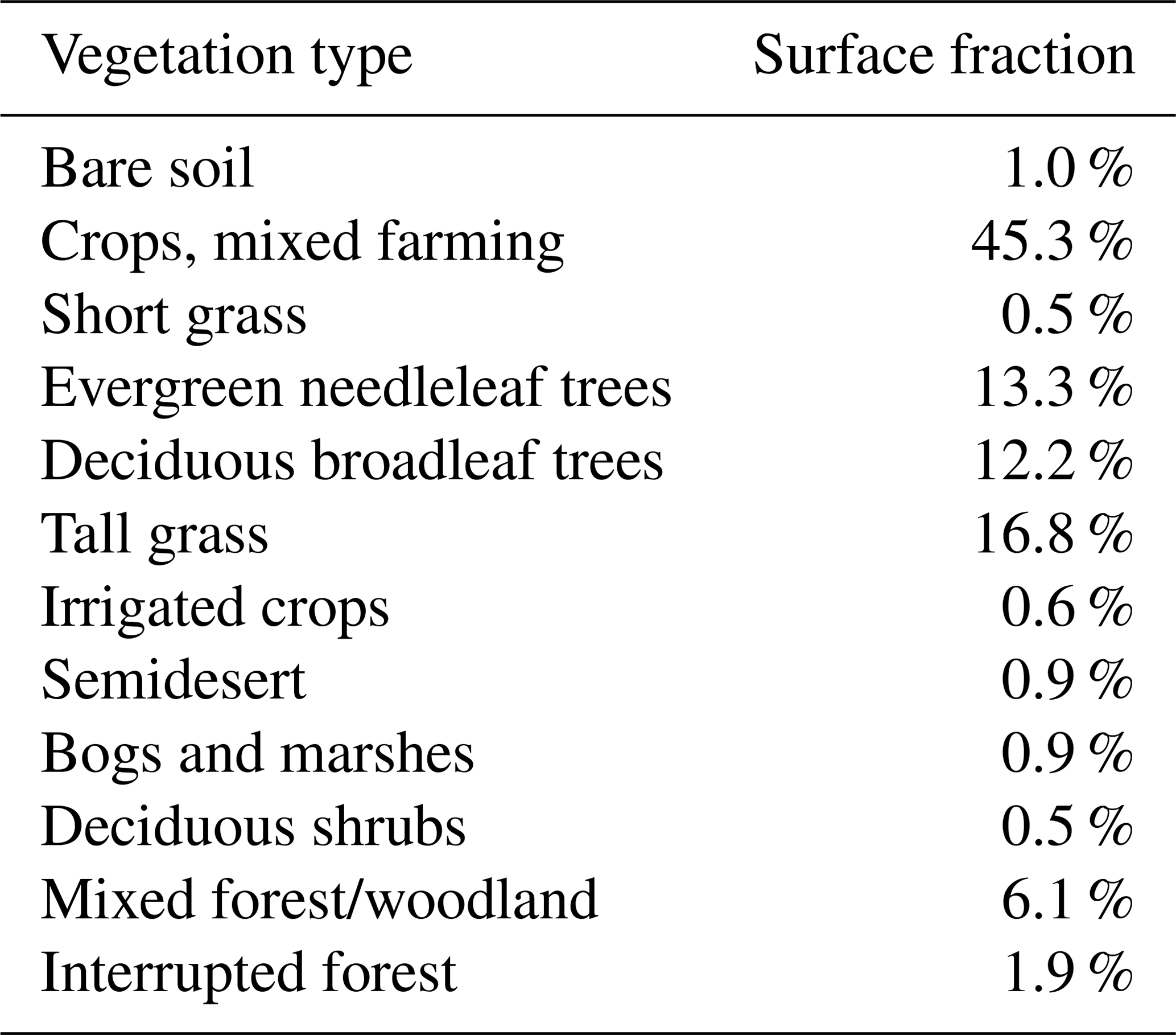
An overview of the atmospheric conditions used to force the main simulations, as derived from the precursor run, are presented in Fig. 2. A relatively typical diurnal cycle of a clear-sky land boundary layer is observed, with slight growth in the boundary layer height observed in daytime and a nocturnal surface inversion. After sunset, super-geostrophic flow is observed following a decrease in mixing. The humidity in the boundary layer increases in daytime due to surface evaporation; this humidity is mixed effectively through the mixed layer, leading to an increase in relative humidity with height.
Table C1Surface parameters of materials as used for the baseline case in the model comparison and with both SLUrb and resolved urban canopies in the model comparison. The values correspond to SLUrb building type 2 and are collected from the works of Oke (1987), Levinson and Akbari (2002), Masson et al. (2002), and Oke et al. (2017).
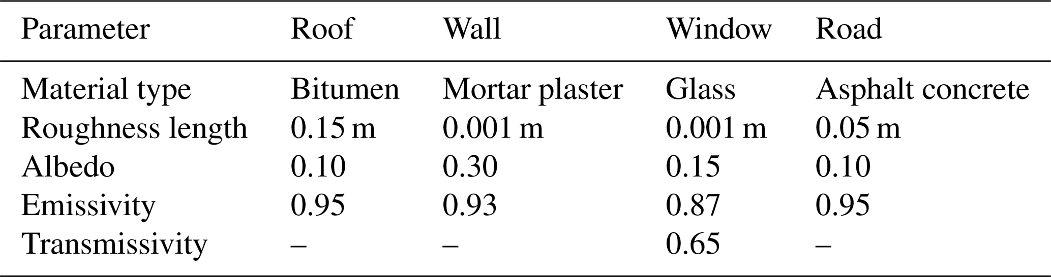
Table C2Thermal parameters of material layers as used for the baseline case in the model comparison and with both SLUrb and resolved urban canopies in the model comparison. The definitions follow German building typology for residential buildings built in 1950–2000 (IWU, 2018; DIN 4108-2, 2013; DIN 4108-4, 2017) and correspond to building type 2 in SLUrb.
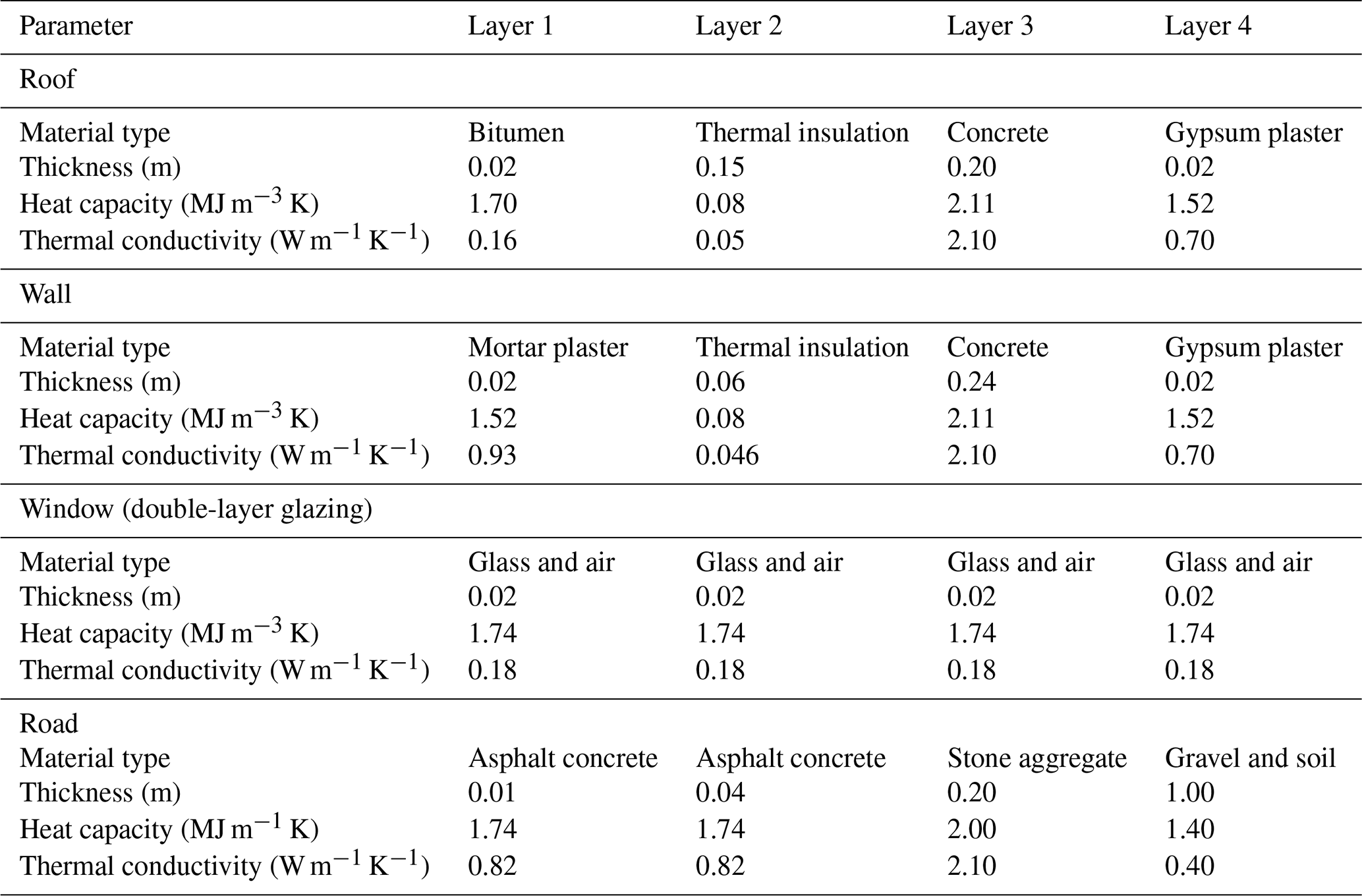
The PALM model system version 24.04 model code used in the sensitivity tests and model comparison, together with the full documentation, is available at https://doi.org/10.5281/zenodo.14221084 (PALM Developers, 2024). The software code used to pre-process, post-process, and analyse data is available at https://doi.org/10.5281/zenodo.14335750 (Karttunen, 2024). The model input and output data are available at https://doi.org/10.23729/f98cce89-a44c-425f-9b73-f591561ce70c (Karttunen and Sühring, 2024).
SK conceptualised the model formulation with the support of LJ and EO. SK wrote the model implementation and official documentation with the support of MS, with MS conducting a thorough review of the code. The model experiments were collaboratively planned by all co-authors, with SK performing the preparation, execution, and analysis. Finally, SK prepared the paper with contributions from all co-authors.
At least one of the (co-)authors is a member of the editorial board of Geoscientific Model Development. The peer-review process was guided by an independent editor, and the authors also have no other competing interests to declare.
Publisher's note: Copernicus Publications remains neutral with regard to jurisdictional claims made in the text, published maps, institutional affiliations, or any other geographical representation in this paper. While Copernicus Publications makes every effort to include appropriate place names, the final responsibility lies with the authors.
The authors are grateful to Siegfried Raasch for the final review of the model implementation. Furthermore, the authors wish to acknowledge CSC – IT Center for Science, Finland, for computational resources. The authors used an AI tool (ChatGPT, GPT-4.5; OpenAI, 2024) to assist with the language editing of an earlier version of this paper. This study was financially supported by the University of Helsinki Doctoral School (UHDS), the Research Council of Finland ACCC Flagship (no. 337549), and the European Union's Horizon 2020 Research and Innovation Programme under grant agreement nos. 101036245, 101037319, and 101135000.
This research has been supported by the Research Council of Finland (grant no. 337549) and EU Horizon 2020 (grant nos. 101036245, 101037319, and 101135000).
Open-access funding was provided by the Helsinki University Library.
This paper was edited by Mohamed Salim and reviewed by three anonymous referees.
Arnfield, A. J.: Two Decades of Urban Climate Research: A Review of Turbulence, Exchanges of Energy and Water, and the Urban Heat Island, Int. J. Climatol., 23, 1–26, https://doi.org/10.1002/joc.859, 2003. a
Baldauf, M.: Stability Analysis for Linear Discretisations of the Advection Equation with Runge–Kutta Time Integration, J. Comput. Phys., 227, 6638–6659, https://doi.org/10.1016/j.jcp.2008.03.025, 2008. a
Barlow, J. F.: Progress in Observing and Modelling the Urban Boundary Layer, Urban Clim., 10, 216–240, https://doi.org/10.1016/j.uclim.2014.03.011, 2014. a, b
Basu, S. and Lacser, A.: A Cautionary Note on the Use of Monin–Obukhov Similarity Theory in Very High-Resolution Large-Eddy Simulations, Bound.-Lay. Meteorol., 163, 351–355, https://doi.org/10.1007/s10546-016-0225-y, 2017. a
Bechtel, B., Alexander, P. J., Böhner, J., Ching, J., Conrad, O., Feddema, J., Mills, G., See, L., and Stewart, I.: Mapping Local Climate Zones for a Worldwide Database of the Form and Function of Cities, ISPRS Int. J. Geo-Inf., 4, 199–219, https://doi.org/10.3390/ijgi4010199, 2015. a
Best, M. J. and Grimmond, C. S. B.: Key Conclusions of the First International Urban Land Surface Model Comparison Project, B. Am. Meteorol. Soc., https://doi.org/10.1175/BAMS-D-14-00122.1, 2015. a
Booten, C., Kruis, N., and Christensen, C.: Identifying and Resolving Issues in EnergyPlus and DOE-2 Window Heat Transfer Calculations, Tech. Rep. NREL/TP-5500-55787, NREL – National Renewable Energy Lab., Golden, CO, USA, https://doi.org/10.2172/1051164, 2012. a
Campanale, A., Adinolfi, M., Raffa, M., Schulz, J.-P., and Mercogliano, P.: Investigating urban heat islands over Rome and Milan during a summer period through the TERRA_URB parameterization in the ICON model, Urban Clim., 60, 102335, https://doi.org/10.1016/j.uclim.2025.102335, 2025. a
Dai, Y., Basu, S., Maronga, B., and de Roode, S. R.: Addressing the Grid-Size Sensitivity Issue in Large-Eddy Simulations of Stable Boundary Layers, Bound.-Lay. Meteorol., 178, 63–89, https://doi.org/10.1007/s10546-020-00558-1, 2021. a, b
Deardorff, J. W.: Stratocumulus-Capped Mixed Layers Derived from a Three-Dimensional Model, Bound.Lay. Meteorol., 18, 495–527, https://doi.org/10.1007/BF00119502, 1980. a, b
Demuzere, M., Hankey, S., Mills, G., Zhang, W., Lu, T., and Bechtel, B.: Combining Expert and Crowd-Sourced Training Data to Map Urban Form and Functions for the Continental US, Sci. Data, 7, 264, https://doi.org/10.1038/s41597-020-00605-z, 2020. a
DIN 4108-2: Wärmeschutz Und Energie-Einsparung in Gebäuden – Teil 2: Mindestanforderungen an Den Wärmeschutz, https://doi.org/10.31030/1929159, 2013. a
DIN 4108-4: Wärmeschutz Und Energie-Einsparung in Gebäuden – Teil 4: Wärme- Und Feuchteschutztechnische Bemessungswerte, https://doi.org/10.31030/2609701, 2017. a
European Environment Agency: CORINE Land Cover 2018 (Raster 100 m), Europe, 6-Yearly, https://doi.org/10.2909/960998c1-1870-4e82-8051-6485205ebbac, 2020. a
Foken, T.: 50 Years of the Monin–Obukhov Similarity Theory, Bound.-Lay. Meteorol., 119, 431–447, https://doi.org/10.1007/s10546-006-9048-6, 2006. a, b
Gehrke, K. F., Sühring, M., and Maronga, B.: Modeling of Land–Surface Interactions in the PALM Model System .0: Land Surface Model Description, First Evaluation, and Sensitivity to Model Parameters, Geosci. Model Dev., 14, 5307–5329, https://doi.org/10.5194/gmd-14-5307-2021, 2021. a, b, c, d, e, f
Gibbs, J. A. and Fedorovich, E.: Sensitivity of Turbulence Statistics in the Lower Portion of a Numerically Simulated Stable Boundary Layer to Parameters of the Deardorff Subgrid Turbulence Model, Q. J. Roy. Meteorol. Soc., 142, 2205–2213, https://doi.org/10.1002/qj.2818, 2016. a
Giorgetta, M. A., Brokopf, R., Crueger, T., Esch, M., Fiedler, S., Helmert, J., Hohenegger, C., Kornblueh, L., Köhler, M., Manzini, E., Mauritsen, T., Nam, C., Raddatz, T., Rast, S., Reinert, D., Sakradzija, M., Schmidt, H., Schneck, R., Schnur, R., Silvers, L., Wan, H., Zängl, G., and Stevens, B.: ICON-A, the Atmosphere Component of the ICON Earth System Model: I. Model Description, J. Adv. Model. Earth Syst., 10, 1613–1637, https://doi.org/10.1029/2017MS001242, 2018. a
Grimmond, C. S. B., Blackett, M., Best, M. J., Barlow, J., Baik, J.-J., Belcher, S. E., Bohnenstengel, S. I., Calmet, I., Chen, F., Dandou, A., Fortuniak, K., Gouvea, M. L., Hamdi, R., Hendry, M., Kawai, T., Kawamoto, Y., Kondo, H., Krayenhoff, E. S., Lee, S.-H., Loridan, T., Martilli, A., Masson, V., Miao, S., Oleson, K., Pigeon, G., Porson, A., Ryu, Y.-H., Salamanca, F., Shashua-Bar, L., Steeneveld, G.-J., Tombrou, M., Voogt, J., Young, D., and Zhang, N.: The International Urban Energy Balance Models Comparison Project: First Results from Phase 1, J. Appl. Meteorol. Clim., 49, https://doi.org/10.1175/2010JAMC2354.1, 2010. a, b
Hackbusch, W.: Multi-Grid Methods and Applications, in: vol. 4 of Springer Series in Computational Mathematics, Springer, Berlin, Heidelberg, ISBN 978-3-642-05722-9, https://doi.org/10.1007/978-3-662-02427-0, 1985. a, b
Harman, I. N. and Finnigan, J. J.: A Simple Unified Theory for Flow in the Canopy and Roughness Sublayer, Bound.-Lay. Meteorol., 123, 339–363, https://doi.org/10.1007/s10546-006-9145-6, 2007. a
Harman, I. N. and Finnigan, J. J.: Scalar Concentration Profiles in the Canopy and Roughness Sublayer, Bound.-Lay. Meteorol., 129, 323–351, https://doi.org/10.1007/s10546-008-9328-4, 2008. a
Heinze, R., Dipankar, A., Henken, C. C., Moseley, C., Sourdeval, O., Trömel, S., Xie, X., Adamidis, P., Ament, F., Baars, H., Barthlott, C., Behrendt, A., Blahak, U., Bley, S., Brdar, S., Brueck, M., Crewell, S., Deneke, H., Di Girolamo, P., Evaristo, R., Fischer, J., Frank, C., Friederichs, P., Göcke, T., Gorges, K., Hande, L., Hanke, M., Hansen, A., Hege, H.-C., Hoose, C., Jahns, T., Kalthoff, N., Klocke, D., Kneifel, S., Knippertz, P., Kuhn, A., van Laar, T., Macke, A., Maurer, V., Mayer, B., Meyer, C. I., Muppa, S. K., Neggers, R. A. J., Orlandi, E., Pantillon, F., Pospichal, B., Röber, N., Scheck, L., Seifert, A., Seifert, P., Senf, F., Siligam, P., Simmer, C., Steinke, S., Stevens, B., Wapler, K., Weniger, M., Wulfmeyer, V., Zängl, G., Zhang, D., and Quaas, J.: Large-Eddy Simulations over Germany Using ICON: A Comprehensive Evaluation, Q. J. Roy. Meteorol. Soc., 143, 69–100, https://doi.org/10.1002/qj.2947, 2017. a
Hellsten, A., Ketelsen, K., Sühring, M., Auvinen, M., Maronga, B., Knigge, C., Barmpas, F., Tsegas, G., Moussiopoulos, N., and Raasch, S.: A Nested Multi-Scale System Implemented in the Large-Eddy Simulation Model PALM Model System 6.0, Geosci. Model Dev., 14, 3185–3214, https://doi.org/10.5194/gmd-14-3185-2021, 2021. a, b
Hersbach, H., Bell, B., Berrisford, P., Hirahara, S., Horányi, A., Muñoz-Sabater, J., Nicolas, J., Peubey, C., Radu, R., Schepers, D., Simmons, A., Soci, C., Abdalla, S., Abellan, X., Balsamo, G., Bechtold, P., Biavati, G., Bidlot, J., Bonavita, M., De Chiara, G., Dahlgren, P., Dee, D., Diamantakis, M., Dragani, R., Flemming, J., Forbes, R., Fuentes, M., Geer, A., Haimberger, L., Healy, S., Hogan, R. J., Hólm, E., Janisková, M., Keeley, S., Laloyaux, P., Lopez, P., Lupu, C., Radnoti, G., de Rosnay, P., Rozum, I., Vamborg, F., Villaume, S., and Thépaut, J.-N.: The ERA5 Global Reanalysis, Q. J. Roy. Meteorol. Soc., 146, 1999–2049, https://doi.org/10.1002/qj.3803, 2020. a, b
Holtslag, A. A. M. and Bruin, H. A. R. D.: Applied Modeling of the Nighttime Surface Energy Balance over Land, J. Appl. Meteorol. Clim., 27, 689–704, https://doi.org/10.1175/1520-0450(1988)027<0689:AMOTNS>2.0.CO;2, 1988. a
Huang, Y., Liu, Y., Liu, Y., Li, H., and Knievel, J. C.: Mechanisms for a Record-Breaking Rainfall in the Coastal Metropolitan City of Guangzhou, China: Observation Analysis and Nested Very Large Eddy Simulation With the WRF Model, J. Geophys. Res.-Atmos., 124, 1370–1391, https://doi.org/10.1029/2018JD029668, 2019. a
IWU – Institut für Wohnen und Umwelt: Deutsche Gebäudetypologie, Institut Wohnen und Umwelt GmbH, Darmstadt, Germany, https://www.iwu.de/publikationen/fachinformationen/gebaeudetypologie/ (last access: 22 May 2025), 2018. a, b
Johnson, G. T., Oke, T. R., Lyons, T. J., Steyn, D. G., Watson, I. D., and Voogt, J. A.: Simulation of Surface Urban Heat Islands under `IDEAL' Conditions at Night Part 1: Theory and Tests against Field Data, Bound.-Lay. Meteorol., 56, 275–294, https://doi.org/10.1007/BF00120424, 1991. a
Kanda, M., Kanega, M., Kawai, T., Moriwaki, R., and Sugawara, H.: Roughness Lengths for Momentum and Heat Derived from Outdoor Urban Scale Models, J. Appl. Meteorol. Clim., 46, 1067–1079, https://doi.org/10.1175/JAM2500.1, 2007. a, b
Karttunen, S.: saskartt/slurb_evaluation: v1.0, Zenodo [code], https://doi.org/10.5281/zenodo.14335750, 2024. a
Karttunen, S. and Sühring, M.: Input and output data for the first PALM-SLUrb v24.04 evaluation, Fairdata [data set], https://doi.org/10.23729/f98cce89-a44c-425f-9b73-f591561ce70c, 2024. a
Krayenhoff, E. S. and Voogt, J. A.: A Microscale Three-Dimensional Urban Energy Balance Model for Studying Surface Temperatures, Bound.-Lay. Meteorol., 123, 433–461, https://doi.org/10.1007/s10546-006-9153-6, 2007. a, b, c, d
Krayenhoff, E. S., Broadbent, A. M., Zhao, L., Georgescu, M., Middel, A., Voogt, J. A., Martilli, A., Sailor, D. J., and Erell, E.: Cooling Hot Cities: A Systematic and Critical Review of the Numerical Modelling Literature, Environ. Res. Lett., 16, 053007, https://doi.org/10.1088/1748-9326/abdcf1, 2021. a
Krč, P., Resler, J., Sühring, M., Schubert, S., Salim, M. H., and Fuka, V.: Radiative Transfer Model 3.0 Integrated into the PALM Model System 6.0, Geosci. Model Dev., 14, 3095–3120, https://doi.org/10.5194/gmd-14-3095-2021, 2021. a, b
Kusaka, H. and Kimura, F.: Coupling a Single-Layer Urban Canopy Model with a Simple Atmospheric Model: Impact on Urban Heat Island Simulation for an Idealized Case, J. Meteorol. Soc. Jpn. Ser. II, 82, 67–80, https://doi.org/10.2151/jmsj.82.67, 2004. a
Le Moigne, P., ed.: SURFEX Scientific Documentation v8.1, in: vol. 3, Météo-France/CNRS, Toulouse, France, https://www.umr-cnrm.fr/surfex/IMG/pdf/surfex_scidoc_v8.1.pdf (last access: 22 May 2025), 2018. a, b
Lemonsu, A., Grimmond, C. S. B., and Masson, V.: Modeling the Surface Energy Balance of the Core of an Old Mediterranean City: Marseille, J. Appl. Meteorol. Clim., https://doi.org/10.1175/1520-0450(2004)043<0312:MTSEBO>2.0.CO;2, 2004. a, b, c, d
Lemonsu, A., Kounkou-Arnaud, R., Desplat, J., Salagnac, J.-L., and Masson, V.: Evolution of the Parisian Urban Climate under a Global Changing Climate, Climatic Change, 116, 679–692, https://doi.org/10.1007/s10584-012-0521-6, 2013. a, b, c, d, e, f, g
Levinson, R. and Akbari, H.: Effects of Composition and Exposure on the Solar Reflectance of Portland Cement Concrete, Cement Concr. Res., 32, 1679–1698, https://doi.org/10.1016/S0008-8846(02)00835-9, 2002. a
Lipson, M. J., Nazarian, N., Hart, M. A., Nice, K. A., and Conroy, B.: A Transformation in City-Descriptive Input Data for Urban Climate Models, Front. Environ. Sci., 10, https://doi.org/10.3389/fenvs.2022.866398, 2022. a
Lipson, M. J., Grimmond, S., Best, M., Abramowitz, G., Coutts, A., Tapper, N., Baik, J.-J., Beyers, M., Blunn, L., Boussetta, S., Bou-Zeid, E., De Kauwe, M. G., de Munck, C., Demuzere, M., Fatichi, S., Fortuniak, K., Han, B.-S., Hendry, M. A., Kikegawa, Y., Kondo, H., Lee, D.-I., Lee, S.-H., Lemonsu, A., Machado, T., Manoli, G., Martilli, A., Masson, V., McNorton, J., Meili, N., Meyer, D., Nice, K. A., Oleson, K. W., Park, S.-B., Roth, M., Schoetter, R., Simón-Moral, A., Steeneveld, G.-J., Sun, T., Takane, Y., Thatcher, M., Tsiringakis, A., Varentsov, M., Wang, C., Wang, Z.-H., and Pitman, A. J.: Evaluation of 30 Urban Land Surface Models in the Urban-PLUMBER Project: Phase 1 Results, Q. J. Roy. Meteorol. Soc., 150, 126–169, https://doi.org/10.1002/qj.4589, 2024. a, b
Macdonald, R. W., Griffiths, R. F., and Hall, D. J.: An Improved Method for the Estimation of Surface Roughness of Obstacle Arrays, Atmos. Environ., 32, 1857–1864, https://doi.org/10.1016/S1352-2310(97)00403-2, 1998. a, b, c, d
Maronga, B., Gryschka, M., Heinze, R., Hoffmann, F., Kanani-Sühring, F., Keck, M., Ketelsen, K., Letzel, M. O., Sühring, M., and Raasch, S.: The Parallelized Large-Eddy Simulation Model (PALM) Version 4.0 for Atmospheric and Oceanic Flows: Model Formulation, Recent Developments, and Future Perspectives, Geosci. Model Dev., 8, 2515–2551, https://doi.org/10.5194/gmd-8-2515-2015, 2015. a, b
Maronga, B., Banzhaf, S., Burmeister, C., Esch, T., Forkel, R., Fröhlich, D., Fuka, V., Gehrke, K. F., Geletič, J., Giersch, S., Gronemeier, T., Groß, G., Heldens, W., Hellsten, A., Hoffmann, F., Inagaki, A., Kadasch, E., Kanani-Sühring, F., Ketelsen, K., Khan, B. A., Knigge, C., Knoop, H., Krč, P., Kurppa, M., Maamari, H., Matzarakis, A., Mauder, M., Pallasch, M., Pavlik, D., Pfafferott, J., Resler, J., Rissmann, S., Russo, E., Salim, M., Schrempf, M., Schwenkel, J., Seckmeyer, G., Schubert, S., Sühring, M., von Tils, R., Vollmer, L., Ward, S., Witha, B., Wurps, H., Zeidler, J., and Raasch, S.: Overview of the PALM Model System 6.0, Geosci. Model Dev., 13, 1335–1372, https://doi.org/10.5194/gmd-13-1335-2020, 2020. a, b, c
Maronga, B., Winkler, M., and Li, D.: Can Areawide Building Retrofitting Affect the Urban Microclimate? An LES Study for Berlin, Germany, J. Appl. Meteorol. Clim., 61, 800–817, https://doi.org/10.1175/JAMC-D-21-0216.1, 2022. a
Martilli, A., Clappier, A., and Rotach, M. W.: An Urban Surface Exchange Parameterisation for Mesoscale Models, Bound.-Lay. Meteorol., 104, 261–304, https://doi.org/10.1023/A:1016099921195, 2002. a, b
Masson, V.: A Physically-Based Scheme For The Urban Energy Budget In Atmospheric Models, Bound.-Lay. Meteorol., 94, 357–397, https://doi.org/10.1023/A:1002463829265, 2000. a, b, c, d, e, f, g, h, i, j, k
Masson, V.: Urban Surface Modeling and the Meso-Scale Impact of Cities, Theor. Appl. Climatol., 84, 35–45, https://doi.org/10.1007/s00704-005-0142-3, 2006. a
Masson, V., Grimmond, C. S. B., and Oke, T. R.: Evaluation of the Town Energy Balance (TEB) Scheme with Direct Measurements from Dry Districts in Two Cities, J. Appl. Meteorol. Clim., https://doi.org/10.1175/1520-0450(2002)041<1011:EOTTEB>2.0.CO;2, 2002. a, b
Meyer, D., Schoetter, R., Riechert, M., Verrelle, A., Tewari, M., Dudhia, J., Masson, V., van Reeuwijk, M., and Grimmond, S.: WRF-TEB: Implementation and Evaluation of the Coupled Weather Research and Forecasting (WRF) and Town Energy Balance (TEB) Model, J. Adv. Model. Earth Syst., 12, e2019MS001961, https://doi.org/10.1029/2019MS001961, 2020. a, b
Monin, A. S. and Obukhov, A. M.: Basic Laws of Turbulent Mixing in the Surface Layer of the Atmosphere, Tr. Akad. Nauk. SSSR Geophiz. Inst., 24, 164–187, 1954. a
Muñoz-Sabater, J., Dutra, E., Agustí-Panareda, A., Albergel, C., Arduini, G., Balsamo, G., Boussetta, S., Choulga, M., Harrigan, S., Hersbach, H., Martens, B., Miralles, D. G., Piles, M., Rodríguez-Fernández, N. J., Zsoter, E., Buontempo, C., and Thépaut, J.-N.: ERA5-Land: A State-of-the-Art Global Reanalysis Dataset for Land Applications, Earth Syst. Sci. Data, 13, 4349–4383, https://doi.org/10.5194/essd-13-4349-2021, 2021. a
Noilhan, J. and Planton, S.: A Simple Parameterization of Land Surface Processes for Meteorological Models, Mon. Weather Rev., 117, https://doi.org/10.1175/1520-0493(1989)117<0536:ASPOLS>2.0.CO;2, 1989. a
Oke, T. R.: Boundary Layer Climates, Taylor & Francis, Routledge, London, in: 2nd Edn., ISBN 978-0-203-40721-9, https://doi.org/10.4324/9780203407219, 1987. a, b
Oke, T. R., Mills, G., Christen, A., and Voogt, J. A.: Urban Climates, Cambridge University Press, Cambridge, ISBN 978-0-521-84950-0, https://doi.org/10.1017/9781139016476, 2017. a, b
OpenAI: ChatGPT: OpenAI Language Model, GPT-4.5, https://chat.openai.com (last access: 22 May 2025, 2024. a
Orlanski, I.: A Simple Boundary Condition for Unbounded Hyperbolic Flows, J. Comput. Phys., 21, 251–269, https://doi.org/10.1016/0021-9991(76)90023-1, 1976. a
PALM Developers: PALM model system 24.04 model code and documentation, Zenodo [code], https://doi.org/10.5281/zenodo.14221084, 2024. a
Paulson, C. A.: The Mathematical Representation of Wind Speed and Temperature Profiles in the Unstable Atmospheric Surface Layer, J. Appl. Meteorol. Clim., 9, 857–861, https://doi.org/10.1175/1520-0450(1970)009<0857:TMROWS>2.0.CO;2, 1970. a
Pfafferott, J., Rißmann, S., Sühring, M., Kanani-Sühring, F., and Maronga, B.: Building indoor model in PALM-4U: indoor climate, energy demand, and the interaction between buildings and the urban microclimate, Geosci. Model Dev., 14, 3511–3519, https://doi.org/10.5194/gmd-14-3511-2021, 2021. a
Pinto, J. O., Jensen, A. A., Jiménez, P. A., Hertneky, T., Muñoz-Esparza, D., Dumont, A., and Steiner, M.: Real-Time WRF Large-Eddy Simulations to Support Uncrewed Aircraft System (UAS) Flight Planning and Operations during 2018 LAPSE-RATE, Earth Syst. Sci. Data, 13, 697–711, https://doi.org/10.5194/essd-13-697-2021, 2021. a
Raasch, S. and Schröter, M.: PALM – A Large-Eddy Simulation Model Performing on Massively Parallel Computers, Meteorol. Z., 10, 363–372, https://doi.org/10.1127/0941-2948/2001/0010-0363, 2001. a
Resler, J., Krč, P., Belda, M., Juruš, P., Benešová, N., Lopata, J., Vlček, O., Damašková, D., Eben, K., Derbek, P., Maronga, B., and Kanani-Sühring, F.: PALM-USM v1.0: A New Urban Surface Model Integrated into the PALM Large-Eddy Simulation Model, Geosci. Model Dev., 10, 3635–3659, https://doi.org/10.5194/gmd-10-3635-2017, 2017. a, b, c
Resler, J., Bauerová, P., Belda, M., Bureš, M., Eben, K., Fuka, V., Geletič, J., Jareš, R., Karel, J., Keder, J., Krč, P., Patiño, W., Radović, J., Řezníček, H., Sühring, M., Šindelářová, A., and Vlček, O.: Challenges of High-Fidelity Air Quality Modeling in Urban Environments – PALM Sensitivity Study during Stable Conditions, Geosci. Model Dev., 17, 7513–7537, https://doi.org/10.5194/gmd-17-7513-2024, 2024. a
Rowley, F. B. and Algren, A. B.: Thermal Conductivity of Building Materials, in: no. 12 in Bulletin of Minnesota Engineering Experiment Station, University of Minnesota, Minnesota, USA, https://hdl.handle.net/11299/124246 (last access: 22 May 2025), 1937. a, b, c
Skamarock, W. C., Klemp, J. B., Dudhia, J., Gill, D. O., Liu, Z., Berner, J., Wang, W., Powers, J. G., Duda, M. G., Barker, D. M., and Huang, X.-Y.: A Description of the Advanced Research WRF Model Version 4, Tech. rep., UCAR/NCAR, https://doi.org/10.5065/1DFH-6P97, 2019. a
Stewart, I. D. and Oke, T. R.: Local Climate Zones for Urban Temperature Studies, B. Am. Meteorol. Soc., 93, https://doi.org/10.1175/BAMS-D-11-00019.1, 2012. a, b
Stiperski, I. and Calaf, M.: Generalizing Monin-Obukhov Similarity Theory (1954) for Complex Atmospheric Turbulence, Phys. Rev. Lett., 130, 124001, https://doi.org/10.1103/PhysRevLett.130.124001, 2023. a
Sullivan, P. P. and Patton, E. G.: The Effect of Mesh Resolution on Convective Boundary Layer Statistics and Structures Generated by Large-Eddy Simulation, J. Atmos. Sci., 68, https://doi.org/10.1175/JAS-D-10-05010.1, 2011. a
Udina, M., Montornès, À., Casso, P., Kosović, B., and Bech, J.: WRF-LES Simulation of the Boundary Layer Turbulent Processes during the BLLAST Campaign, Atmosphere, 11, 1149, https://doi.org/10.3390/atmos11111149, 2020. a
US Department of Energy: EnergyPlus™ Version 24.1.0, https://energyplus.net/assets/nrel_custom/pdfs/pdfs_v24.1.0/pdfs.zip (last access: 22 May 2025), 2024. a
Wang, Y., Ma, Y.-F., Muñoz-Esparza, D., Dai, J., Li, C. W. Y., Lichtig, P., Tsang, R. C.-W., Liu, C.-H., Wang, T., and Brasseur, G. P.: Coupled Mesoscale–Microscale Modeling of Air Quality in a Polluted City Using WRF-LES-Chem, Atmos. Chem. Phys., 23, 5905–5927, https://doi.org/10.5194/acp-23-5905-2023, 2023. a
Wicker, L. J. and Skamarock, W. C.: Time-Splitting Methods for Elastic Models Using Forward Time Schemes, Mon. Weather Rev., 130, 2088–2097, https://doi.org/10.1175/1520-0493(2002)130<2088:TSMFEM>2.0.CO;2, 2002. a, b
Williamson, J. H.: Low-Storage Runge-Kutta Schemes, J. Comput. Phys., 35, 48–56, https://doi.org/10.1016/0021-9991(80)90033-9, 1980. a, b, c
Wurps, H., Steinfeld, G., and Heinz, S.: Grid-Resolution Requirements for Large-Eddy Simulations of the Atmospheric Boundary Layer, Bound.-Lay. Meteorol., 175, 179–201, https://doi.org/10.1007/s10546-020-00504-1, 2020. a
Xie, Z. and Castro, I. P.: LES and RANS for Turbulent Flow over Arrays of Wall-Mounted Obstacles, Flow Turbul. Combust., 76, 291–312, https://doi.org/10.1007/s10494-006-9018-6, 2006. a
Zängl, G., Reinert, D., Rípodas, P., and Baldauf, M.: The ICON (ICOsahedral Non-hydrostatic) Modelling Framework of DWD and MPI-M: Description of the Non-Hydrostatic Dynamical Core, Q. J. Roy. Meteorol. Soc., 141, 563–579, https://doi.org/10.1002/qj.2378, 2015. a
Zhong, J., Nikolova, I., Cai, X., MacKenzie, A. R., Alam, M. S., Xu, R., Singh, A., and Harrison, R. M.: Neighbourhood-Scale Dispersion of Traffic-Induced Ultrafine Particles in Central London: WRF Large Eddy Simulations, Environ. Pollut., 266, 115223, https://doi.org/10.1016/j.envpol.2020.115223, 2020. a
Zhu, X., Li, D., Zhou, W., Ni, G., Cong, Z., and Sun, T.: An Idealized LES Study of Urban Modification of Moist Convection, Q. J. Roy. Meteorol. Soc., 143, 3228–3243, https://doi.org/10.1002/qj.3176, 2017. a
- Abstract
- Introduction
- Model description
- Sensitivity tests
- Model comparison
- Limitations and development outlook
- Conclusions
- Appendix A: Longwave radiative budgets
- Appendix B: Precursor setup
- Appendix C: Material parameters
- Code and data availability
- Author contributions
- Competing interests
- Disclaimer
- Acknowledgements
- Financial support
- Review statement
- References