Accelerated pseudo-transient method for elastic, viscoelastic, and coupled hydromechanical problems with applications

The accelerated pseudo-transient (APT) method is a matrix-free approach used to solve partial differential equations (PDEs), characterized by its reliance on local operations, which makes it highly suitable for parallelization. With the advent of the memory-wall phenomenon around 2005, where memory access speed overtook floating-point operations as the bottleneck in high-performance computing, the APT method has gained prominence as a powerful tool for tackling various PDEs in geosciences. Recent advancements have demonstrated the APT method's computational efficiency, particularly when applied to quasi-static nonlinear problems using Graphical Processing Units (GPUs). This study presents a comprehensive analysis of the APT method, focusing on its application to quasi-static elastic, viscoelastic, and coupled hydromechanical problems, specifically those governed by quasi-static Biot poroelastic equations, across 1D, 2D, and 3D domains. We systematically investigate the optimal numerical parameters required to achieve rapid convergence, offering valuable insights into the method's applicability and efficiency for a range of physical models. Our findings are validated against analytical solutions, underscoring the robustness and accuracy of the APT method in both homogeneous and heterogeneous media. We explore the influence of boundary conditions, nonlinearities, and coupling on the optimal convergence parameters, highlighting the method's adaptability in addressing complex and realistic scenarios. To demonstrate the flexibility of the APT method, we apply it to the nonlinear mechanical problem of strain localization using a poro-elasto-viscoplastic rheological model, achieving extremely high resolutions – 10 000² in 2D and 512³ in 3D – that, to our knowledge, have not been previously explored for such models. Our study contributes significantly to the field by providing a robust framework for the effective implementation of the APT method in solving challenging geophysical problems. Importantly, the results presented in this paper are fully reproducible, with MATLAB code, symbolic Maple scripts, and CUDA C codes made available in a permanent repository.

1 Introduction

The accelerated pseudo-transient (APT) method represents a powerful tool in computational science, combining efficiency, scalability, ease of implementation, and a strong theoretical foundation rooted in wave physics. The main idea of the APT method is that instead of solving the original partial differential equation (PDE), a modified PDE with added inertial terms and attenuation is solved in an iterative fashion until the inertial terms vanish. In other words, the solution of the original PDE is an attractor of the transient PDE with inertia.

The accelerated pseudo-transient (APT) method is designed to iteratively solve a modified version of the original partial differential equation (PDE) by introducing inertial and relaxation terms. This modified PDE is repeatedly solved until the added pseudo-physical terms vanish, providing an accurate approximation of the solution to the original equation. The APT method becomes increasingly efficient when implemented with exclusively spatially local operations, eliminating the need to access global storage for evolving fields. Unlike the conjugate gradient method, which requires two global scalar products per iteration, the APT method advances without global memory operations, enhancing computational performance by utilizing fast cache memory. This method is versatile, applicable to both linear and nonlinear equations, and distinguishes itself with several key attributes. (i) APT is a matrix-free method, enabling the solution of large-scale 3D problems without the overhead of matrix storage. (ii) Leveraging only local operations, APT naturally lends itself to parallelization, making it well-suited for modern computing architectures. (iii) Its structure facilitates efficient implementation on Graphical Processing Units (GPUs), capitalizing on their ability to handle parallel tasks efficiently. (iv) The APT method aligns closely with the physics of wave phenomena, offering a robust theoretical framework for rigorous understanding and application.

One of the first pseudo-transient (PT) iterative methods to solve elliptic PDEs was presented by Richardson (1911). An improved PT method for elliptic problems, which can be referred to as the accelerated pseudo-transient (APT) method, was proposed in the 1950s by Frankel (1950) and further investigated by Riley (1954) and Young (1972). The pseudo-transient method is also known as a dynamic relaxation (DR) method that was used by Otter (1965) and Otter et al. (1966). Interestingly, the APT method was also applied in other branches of science, e.g., in areas related to optimization problems (Polyak, 1964). In geosciences, the APT method was introduced as the Fast Lagrangian Analysis of Continua (FLAC) algorithm by Cundall (1976), and it was applied to solve nonlinear problems and instabilities (Poliakov et al., 1993a, 1994). The APT method was recently applied to model large 3D geophysical problems: coupled two-phase flow physics represented by solitary porosity waves (Räss et al., 2019), reaction-driven porosity waves (Omlin et al., 2017), and thermomechanical ice deformation (Räss et al., 2020). The APT method was applied to model focused fluid flow by Wang et al. (2022). Furthermore, Wang et al. (2022) investigated the physics-based principles underlying the APT method. A compaction-driven fluid flow and plasticity within porous media were investigated numerically by Alkhimenkov et al. (2024a). A numerical approach based on GPUs to model the strain localization in 2D and 3D of a (visco)-hypoelastic–perfectly plastic medium was developed by Alkhimenkov et al. (2024b).

The efficiency of the APT method strongly depends on the choice of the numerical parameters. For simple equations, such parameters can be derived analytically. This was done for elliptic equations by analyzing a damped wave equation (DWE) (Cox and Zuazua, 1994), since the solution of elliptic equations is an attractor of DWE. In optimization problems the APT method is also known as a PDE acceleration framework (Calder and Yezzi, 2019; Benyamin et al., 2020). A comprehensive study that provides the optimal values of numerical parameters of the APT method for various problems is provided by Räss et al. (2022). Such problems include diffusion–reaction equations, transient diffusion, incompressible viscous shear-driven Couette flow, and the incompressible viscous and viscoelastic Stokes equation. Remarkably, the APT method can be applied to other classes of problems that are described in the present paper.

The present study provides a comprehensive study of the application of the APT method to compressible quasi-static elastic and viscoelastic equations and to coupled hydromechanical problems represented by the quasi-static Biot poroelastic equations.

The novelties of this paper are summarized as follows.

1. A set of optimal parameters tailored for compressible quasi-static elastic and viscoelastic equations is presented.

2. Validation against analytical solutions is conducted to verify the accuracy of the APT solutions of quasi-static elasticity equations.

3. A new set of optimal parameters specifically designed for coupled hydromechanical problems, represented by the quasi-static Biot poroelastic equations, is introduced.

4. Applications of the APT method are presented for ultrahigh-resolution simulations of 10 000² in 2D and 512³ in 3D for poro-elasto-plastic equations.

2 Mathematical formulation: quasi-static elasticity equations

2.1 General form

Consider a domain V in a three-dimensional Euclidean space E³ bounded by a regular surface ∂V. The equilibrium equation (conservation of linear momentum under the conditions of equilibrium and neglecting body forces) is (Landau and Lifshitz, 1959; Nemat-Nasser and Hori, 2013)

$$\begin{array}{}\text{(1)}& \mathbf{\nabla }\cdot \mathit{\sigma }=\mathrm{0},\end{array}$$

where σ is stress tensor, ⋅ is the dot product, ∇ is the del operator, and ∇⋅ is the divergence operator. The del operator, ∇, is a vectorial differential operator, denoted by Li and Wang (2008) and Nemat-Nasser and Hori (2013) as $\mathbf{\nabla }\equiv {\partial }_i{\mathit{e}}_i\equiv \partial {\mathit{e}}_i/\partial x_i$, where e_i represents the base vectors and x_i represents the coordinates. The stress tensor σ can be decomposed into pressure (minus the mean stress), p, and the deviatoric stress tensor, τ, such that $\mathit{\sigma }=-p{\mathbf{I}}_{\mathrm{2}}+\mathit{\tau },$ where I₂ is the second-order identity tensor. In a rate formulation, the constitutive equation (the stress rate–velocity relation) is

$$\begin{array}{}\text{(2)}& {\displaystyle \frac{\partial \mathit{\sigma }\left(\mathit{v}\right)}{\partial t}}=\mathbf{C}:{\displaystyle \frac{\partial \mathit{\epsilon }}{\partial t}},\text{(3)}& {\displaystyle \frac{\partial \mathit{\epsilon }}{\partial t}}={\displaystyle \frac{\mathrm{1}}{\mathrm{2}}}\left(\mathbf{\nabla }\otimes \mathit{v}+(\mathbf{\nabla }\otimes \mathit{v}{)}^{\text{T}}\right),\end{array}$$

where C is the fourth rank stiffness tensor (with components C_ijkl), “:” is the double-dot product, ⊗ is the tensor product, the superscript T denotes transpose, $\partial \mathit{\epsilon }/\partial t$ is the strain rate tensor, and v is the velocity field. For the elasticity problems, we consider two different tasks: (i) loading and unloading of an elastic body and (ii) calculation of effective elastic properties.

2.2 1D elasticity equations

For simplicity, we consider 1D elasticity equations. We consider the following system of equations:

$$\begin{array}{}\text{(4)}& \left\{\begin{array}{l}\frac{\partial {\mathit{\sigma }}_{xx}}{\partial t}=(K+\frac{\mathrm{4}}{\mathrm{3}}G)\frac{\partial v_x}{\partial x}\\ \mathrm{0}=\frac{\partial {\mathit{\sigma }}_{xx}}{\partial x},\end{array}\right.\end{array}$$

where σ_xx is the component of the stress tensor, v_x is the velocity, K is the bulk modulus, and G is the shear modulus. Note that the system in Eq. (4) is a 1D version of the full system of elasticity in Eqs. (1)–(3).

2.2.1 Problem statement

The system in Eqs. (1)–(3) can be applied to solve many problems in solid mechanics. Particularly, as an example in this study, we use these equations to solve two applied problems: (i) loading and unloading of an elastic body and (ii) calculation of effective elastic properties.

For the analysis of loading and unloading processes in an elastic body, the system in Eq. (4) is discretized with a physical time step Δt, which is intrinsically linked to specific strain increments. The loading and unloading process is simulated through a series of time increments, cumulatively spanning the total time of interest. This total time corresponds to the overall strain accumulation within the elastic body. In contrast, when computing effective elastic properties (task ii), the system in Eq. (4) is utilized with a single loading increment, characterized by a physical time step Δt. This solitary increment corresponds to a single strain loading step. Subsequently, the stress and strain fields are spatially averaged across the model domain. The division of these averaged quantities yields the effective elastic moduli.

2.3 The pseudo-transient method

The pseudo-transient (PT) method is used to solve the system in Eq. (4) (Frankel, 1950; Räss et al., 2022). The pseudo-transient method is matrix-free and builds on a transient physics analogy to establish a stationary solution. The main idea is that the solution of a quasi-static equation (stationary process), usually described by an elliptic PDE, is represented by an attractor of a transient process described by parabolic or hyperbolic PDEs. Simply put, the equations are written in their residual form, and pseudo-time derivatives are added to the left-hand side. The solution is achieved once the pseudo-time derivatives attenuate to a certain precision (e.g., 10⁻¹²). An overview of the first simplified versions of the PT and APT methods is given in Appendix A.

2.3.1 The accelerated pseudo-transient method: modern version

Here we report a modern version of the APT method. The solution of the quasi-static elasticity equations can be achieved in two steps. (i) Inertial terms are added into the constitutive relations. (ii) Inertial terms are responsible for wave propagation in pseudo-physical time and space (i.e., hyperbolic), and viscous terms (treated as a Maxwell rheology) are the physical quantities. The quasi-static elasticity in Eq. (4) can then be rewritten with the pseudo-time $\stackrel{\mathrm{̃}}{t}$,

$$\begin{array}{}\text{(5)}& \left\{\begin{array}{l}\frac{\mathrm{1}}{\stackrel{\mathrm{̃}}{H}}\frac{\partial {\mathit{\sigma }}_{xx}}{\partial \stackrel{\mathrm{̃}}{t}}+\frac{\mathrm{1}}{H}\frac{{\mathit{\sigma }}_{xx}-{\widehat{\mathit{\sigma }}}_{xx}}{\mathrm{\Delta }t}=\frac{\partial v_x}{\partial x}\\ \stackrel{\mathrm{̃}}{\mathit{\rho }}\frac{\partial v_x}{\partial \stackrel{\mathrm{̃}}{t}}=\frac{\partial {\mathit{\sigma }}_{xx}}{\partial x},\end{array}\right.\end{array}$$

where ${\widehat{\mathit{\sigma }}}_{xx}$ is the stress field at the previous physical time step and $C_{\mathrm{1111}}=\stackrel{\mathrm{̃}}{H}\equiv H=K+\frac{\mathrm{4}}{\mathrm{3}}G$ is the P-wave modulus. For example, the system (Eq. 5) can be solved for the case of elastic loading and unloading where the stress ${\widehat{\mathit{\sigma }}}_{xx}$ is nonzero from the previous physical time step.

For the analysis of the system in Eq. (5) we can omit $\widehat{\mathit{\sigma }}$ since the stress $\widehat{\mathit{\sigma }}$ does not change inside the loop over pseudo-time $\stackrel{\mathrm{̃}}{t}$:

$$\begin{array}{}\text{(6)}& \left\{\begin{array}{l}\frac{\mathrm{1}}{\stackrel{\mathrm{̃}}{H}}\frac{\partial {\mathit{\sigma }}_{xx}}{\partial \stackrel{\mathrm{̃}}{t}}+\frac{\mathrm{1}}{H}\frac{{\mathit{\sigma }}_{xx}}{\mathrm{\Delta }t}=\frac{\partial v_x}{\partial x}\\ \stackrel{\mathrm{̃}}{\mathit{\rho }}\frac{\partial v_x}{\partial \stackrel{\mathrm{̃}}{t}}=\frac{\partial {\mathit{\sigma }}_{xx}}{\partial x}.\end{array}\right.\end{array}$$

In the system in Eq. (5) (or Eq. 6), $\stackrel{\mathrm{̃}}{\mathit{\rho }}$ is a to-be-determined numerical parameter. For the analysis of the optimal numerical parameters, the systems in Eqs. (5) and (6) are equivalent to each other since the quantity ${\widehat{\mathit{\sigma }}}_{xx}$ is constant during the iterations over the pseudo-time $\stackrel{\mathrm{̃}}{t}$.

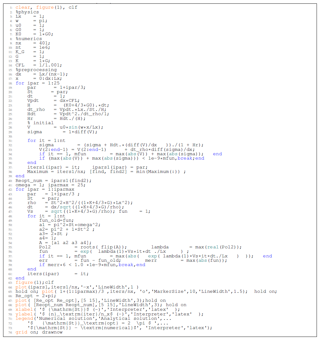
The APT version of the expression in Eq. (5) (or Eq. 6), where the stress tenor is decomposed into the pressure and deviatoric stress tensor, is provided in Appendix B, and a discrete version of the system in Eq. (6) is provided in Appendix C. A MATLAB routine to solve the system in Eq. (6) is presented in Appendix D.

The system in Eq. (6) is hyperbolic and corresponds to a wave propagation in a dissipative medium. The numerical parameters in the system (Eq. 6) determine the attenuation of propagating waves. Our target is to solve elasticity equations that are quasi-static. Therefore, the goal is to find optimal values of the numerical parameters that correspond to the fastest attenuation of propagating waves. More precisely, once the pseudo-time derivatives ($\partial {\mathit{\sigma }}_{xx}/\partial \stackrel{\mathrm{̃}}{t}$, $\partial v_x/\partial \stackrel{\mathrm{̃}}{t}$) in the system (Eq. 6) disappear, the resulting solution of the quasi-static equations is found. In other words, the solution to quasi-static equations in an attractor of the system in Eq. (6) at large “pseudo”-timescales. For a particular (optimal) choice of the numerical parameters, the attractor solution can be achieved faster than by using nonoptimal values of the numerical parameters. In the best scenario, the number of iterations n_I needed to converge to the target solution is n_I∼n_x, more precisely n_I=k n_x, where usually k is in a range of $k\in [\mathrm{5};\mathrm{50}]$ (the lower and upper bounds provided must be considered an approximation). In other words, the wave travels several times throughout the whole domain before the corresponding updates of the time derivatives attenuate to a desired precision. If nonoptimal parameters are used, the solution may not converge for a long computational time.

Let us describe some basic features of the system in Eq. (6). The “numerical” primary or P-wave velocity can be defined as

$$\begin{array}{}\text{(7)}& {\stackrel{\mathrm{̃}}{V}}_{\mathrm{p}}=\sqrt{{\displaystyle \frac{\stackrel{\mathrm{̃}}{H}}{\stackrel{\mathrm{̃}}{\mathit{\rho }}}}}.\end{array}$$

The Courant–Friedrichs–Lewy (CFL) condition for the system in Eq. (6) suggests that (Alkhimenkov et al., 2021a)

$$\begin{array}{}\text{(8)}& \mathrm{\Delta }\stackrel{\mathrm{̃}}{t}\le {\displaystyle \frac{\mathrm{\Delta }x}{{\stackrel{\mathrm{̃}}{V}}_{\mathrm{p}}}}\text{or}\mathrm{\Delta }\stackrel{\mathrm{̃}}{t}={\displaystyle \frac{\stackrel{\mathrm{̃}}{C}\mathrm{\Delta }x}{{\stackrel{\mathrm{̃}}{V}}_{\mathrm{p}}}},\end{array}$$

where $\stackrel{\mathrm{̃}}{C}\le \mathrm{1}$. Note that the system in Eq. (6) is identical to the damped linear wave equation and the CFL condition (Eq. 8) is just a lower bound (Alkhimenkov et al., 2021a). It is important to mention that we do not need to know the optimal values of all the numerical parameters separately. Instead, the following combinations are needed for the numerical implementation of the APT algorithm: $\stackrel{\mathrm{̃}}{H}\mathrm{\Delta }\stackrel{\mathrm{̃}}{t}$ and $\mathrm{\Delta }\stackrel{\mathrm{̃}}{t}/\stackrel{\mathrm{̃}}{\mathit{\rho }}$.

Let us analyze the system in Eq. (6). First, we perform a dispersion analysis. A solution of traveling waves in dissipative media can be written as

$$\begin{array}{}\text{(9)}& F(\stackrel{\mathrm{̃}}{t},x)=\exp \left[{\displaystyle \frac{(\mathit{\gamma }{\stackrel{\mathrm{̃}}{V}}_{\mathrm{p}}\stackrel{\mathrm{̃}}{t}+\mathit{\pi }\mathit{\omega }xi)}{L_x}}\right],\end{array}$$

where γ is the amplitude, ω=2 π f is the angular frequency (f is the frequency), i is the imaginary unit, and in our description $\exp [\cdot ]\equiv e^{(\cdot )}$. The amplification matrix F of this system is a 2×2 matrix (Hirsch, 1988; Alkhimenkov et al., 2021a):

$$\begin{array}{}\text{(10)}& F=\left[\begin{array}{cc}\frac{\mathit{\gamma }\mathrm{\Delta }x}{L_x}& \frac{-\mathrm{3}i\mathit{\pi }\mathrm{\Delta }x}{\mathrm{7}\mathit{St}}\\ \frac{-\mathrm{7}\mathrm{\Delta }x\mathit{St}\mathit{\pi }}{\mathrm{3}{L}_x^{\mathrm{2}}}& \frac{\mathrm{\Delta }x(\mathit{St}+\mathit{\gamma })}{L_x}\end{array}\right],\end{array}$$

where the dimensionless parameter, the Strouhal number, St, is expressed as

$$\begin{array}{}\text{(11)}& \mathit{St}={\displaystyle \frac{L_x}{{\stackrel{\mathrm{̃}}{V}}_{\mathrm{p}}\mathrm{\Delta }t}}.\end{array}$$

The discriminant D of the matrix (Eq. 10) is

$$\begin{array}{}\text{(12)}& D=\left({\mathit{\gamma }}^{\mathrm{2}}+\mathit{St}\mathit{\gamma }+{\mathit{\pi }}^{\mathrm{2}}\right){\left({\displaystyle \frac{\mathrm{\Delta }x}{L_x}}\right)}^{\mathrm{2}}.\end{array}$$

Setting D=0 and solving for γ, we get two roots:

$$\begin{array}{}\text{(13)}& {\displaystyle }{\mathit{\gamma }}_{\mathrm{1}}=-{\displaystyle \frac{\mathit{St}}{\mathrm{2}}}+{\displaystyle \frac{\sqrt{-\mathrm{4}{\mathit{\pi }}^{\mathrm{2}}+{\mathit{St}}^{\mathrm{2}}}}{\mathrm{2}}},\text{(14)}& {\displaystyle }{\mathit{\gamma }}_{\mathrm{2}}=-{\displaystyle \frac{\mathit{St}}{\mathrm{2}}}-{\displaystyle \frac{\sqrt{-\mathrm{4}{\mathit{\pi }}^{\mathrm{2}}+{\mathit{St}}^{\mathrm{2}}}}{\mathrm{2}}}.\end{array}$$

The real parts of the roots (γ₁ and γ₂) control the exponential decay rate of the solution (Räss et al., 2022); therefore, we are interested in the minimum of these values. This minimum reaches its value when the discriminant is zero:

$$\begin{array}{}\text{(15)}& -\mathrm{4}{\mathit{\pi }}^{\mathrm{2}}+{\mathit{St}}^{\mathrm{2}}=\mathrm{0}.\end{array}$$

The resulting solution for St has two roots: 2π and −2π. Taking the positive root we get

$$\begin{array}{}\text{(16)}& \mathit{St}={\mathit{St}}_{\text{opt}}=\mathrm{2}\mathit{\pi },\end{array}$$

which is the optimal value of the numerical parameter St that corresponds to the fastest attenuation of propagating waves.

There is only one numerical parameter that controls the dissipation and convergence to the target solution of the quasi-static equations: the Strouhal number, St, which is a purely numerical parameter in our analysis and can be chosen to be arbitrary. For St≪1 the system in Eq. (6) behaves as purely hyperbolic without the stiff source term; in other words, propagating waves do not attenuate (especially when St→0). In contrast, for St≫1 the system in Eq. (6) behaves as hyperbolic with the stiff source term that dominates; therefore, the system in Eq. (6) behaves as a diffusion process and attenuates very slowly. The optimal choice of the Strouhal number, St, is between these two limits: $\mathit{St}={\mathit{St}}_{\text{opt}}=\mathrm{2}\mathit{\pi }$ as shown by the expression in Eq. (16).

Let us do some transformations with the expression in Eq. (11). Our goal is to separate the numerical combination $\mathrm{\Delta }\stackrel{\mathrm{̃}}{t}/\stackrel{\mathrm{̃}}{\mathit{\rho }}$ on the left-hand side and the other variables on the right-hand side,

$$\begin{array}{}\text{(17)}& \begin{array}{rl}\mathrm{1}& ={\displaystyle \frac{L_x}{\mathit{St}{\stackrel{\mathrm{̃}}{V}}_{\mathrm{p}}\mathrm{\Delta }t}}⟺\mathrm{1}={\displaystyle \frac{L_x\sqrt{\stackrel{\mathrm{̃}}{\mathit{\rho }}}}{\mathit{St}\sqrt{\stackrel{\mathrm{̃}}{H}}\mathrm{\Delta }t}}{\displaystyle \frac{\sqrt{\stackrel{\mathrm{̃}}{\mathit{\rho }}}\mathrm{\Delta }\stackrel{\mathrm{̃}}{t}}{\sqrt{\stackrel{\mathrm{̃}}{\mathit{\rho }}}\mathrm{\Delta }\stackrel{\mathrm{̃}}{t}}}⟺{\displaystyle \frac{\mathrm{\Delta }\stackrel{\mathrm{̃}}{t}}{\stackrel{\mathrm{̃}}{\mathit{\rho }}}}\\ & ={\displaystyle \frac{L_x\mathrm{\Delta }\stackrel{\mathrm{̃}}{t}}{\mathit{St}\sqrt{\stackrel{\mathrm{̃}}{H}}\sqrt{\stackrel{\mathrm{̃}}{\mathit{\rho }}}\mathrm{\Delta }t}}{\displaystyle \frac{{\stackrel{\mathrm{̃}}{V}}_{\mathrm{p}}}{{\stackrel{\mathrm{̃}}{V}}_{\mathrm{p}}}},\end{array}\end{array}$$

and continue with

$$\begin{array}{}\text{(18)}& {\displaystyle \frac{\mathrm{\Delta }\stackrel{\mathrm{̃}}{t}}{\stackrel{\mathrm{̃}}{\mathit{\rho }}}}={\displaystyle \frac{{\stackrel{\mathrm{̃}}{V}}_{\mathrm{p}}\mathrm{\Delta }\stackrel{\mathrm{̃}}{t}{L}_x}{\mathit{St}\stackrel{\mathrm{̃}}{H}\mathrm{\Delta }t}}.\end{array}$$

By using the expression in Eq. (8), we determine that ${\stackrel{\mathrm{̃}}{V}}_{\mathrm{p}}\mathrm{\Delta }\stackrel{\mathrm{̃}}{t}=\stackrel{\mathrm{̃}}{C}\mathrm{\Delta }x$; therefore, Eq. (18) can be rewritten as

$$\begin{array}{}\text{(19)}& {\displaystyle \frac{\mathrm{\Delta }\stackrel{\mathrm{̃}}{t}}{\stackrel{\mathrm{̃}}{\mathit{\rho }}}}={\displaystyle \frac{\stackrel{\mathrm{̃}}{C}\mathrm{\Delta }x{L}_x}{\mathit{St}\stackrel{\mathrm{̃}}{H}\mathrm{\Delta }t}}.\end{array}$$

In the expression in Eq. (19), all the parameters on the right-hand side are known; thus $\mathrm{\Delta }\stackrel{\mathrm{̃}}{t}/\stackrel{\mathrm{̃}}{\mathit{\rho }}$ can be evaluated. Now let us create an expression for the second numerical combination, $\stackrel{\mathrm{̃}}{H}\mathrm{\Delta }\stackrel{\mathrm{̃}}{t}$. For that we employ the following transformations:

$$\begin{array}{}\text{(20)}& \begin{array}{rl}\mathrm{1}& ={\displaystyle \frac{{\stackrel{\mathrm{̃}}{V}}_{\mathrm{p}}^{\mathrm{2}}\mathrm{\Delta }{\stackrel{\mathrm{̃}}{t}}^{\mathrm{2}}}{{\stackrel{\mathrm{̃}}{V}}_{\mathrm{p}}^{\mathrm{2}}\mathrm{\Delta }{\stackrel{\mathrm{̃}}{t}}^{\mathrm{2}}}}⟺{\displaystyle \frac{{\stackrel{\mathrm{̃}}{V}}_{\mathrm{p}}^{\mathrm{2}}\stackrel{\mathrm{̃}}{\mathit{\rho }}\mathrm{\Delta }{\stackrel{\mathrm{̃}}{t}}^{\mathrm{2}}}{\stackrel{\mathrm{̃}}{H}\mathrm{\Delta }{\stackrel{\mathrm{̃}}{t}}^{\mathrm{2}}}}⟺\stackrel{\mathrm{̃}}{H}\mathrm{\Delta }\stackrel{\mathrm{̃}}{t}\\ & =({\stackrel{\mathrm{̃}}{V}}_{\mathrm{p}}\mathrm{\Delta }\stackrel{\mathrm{̃}}{t}{)}^{\mathrm{2}}{\left({\displaystyle \frac{\mathrm{\Delta }\stackrel{\mathrm{̃}}{t}}{\stackrel{\mathrm{̃}}{\mathit{\rho }}}}\right)}^{-\mathrm{1}}.\end{array}\end{array}$$

Note that ${\stackrel{\mathrm{̃}}{V}}_{\mathrm{p}}\mathrm{\Delta }\stackrel{\mathrm{̃}}{t}$ and $\mathrm{\Delta }\stackrel{\mathrm{̃}}{t}/\stackrel{\mathrm{̃}}{\mathit{\rho }}$ are already defined above; therefore, it is straightforward to calculate $\stackrel{\mathrm{̃}}{H}\mathrm{\Delta }\stackrel{\mathrm{̃}}{t}$. Therefore, the system of equations in Eq. (5) (or Eq. 6) or its discrete version (Eq. C1) can be solved.

2.4 Problem statement: validation of the numerical parameters

To validate the numerical parameters, the following experiment is performed: in the numerical solver, we set all boundary conditions to zero and initialize the system with a sinusoidal wave. The numerical solution is then run over pseudo-time until it converges to a specified precision (i.e., 10⁻¹²). Simultaneously, the same equation is solved using the analytical method (amplification matrix) to achieve the same precision (i.e., 10⁻¹²). The results are then compared as a function of St. Ideally, the results should be identical or very close, which would validate the choice of numerical parameters and the applied numerical scheme. For the numerical solution, we use a classical conservative staggered space–time grid discretization (Virieux, 1986), which is equivalent to a finite-volume approach (Dormy and Tarantola, 1995). More details on the present discretization can be found in Alkhimenkov et al. (2021b, a).

2.5 Applications of the APT method

To demonstrate the effectiveness and robustness of the APT method, we provide several applications, including the calculation of the convergence rate, the determination of effective elastic properties in homogeneous and heterogeneous media, and comparisons against analytical solutions.

2.5.1 Numerical experiment 1: convergence rate in a homogeneous medium

Figure 1 shows the numerical and analytical results for the system in Eq. (6) (see explanation in Sect. 2.4). The numerical results correspond to the solution with different St numbers until the update of the pseudo-time derivatives becomes less than 10⁻⁹. The analytical result corresponds to the analytical solution of the dispersion relations as a function of St. It can be seen that the analytical and numerical results are in excellent agreement (Fig. 1), which validates the proposed approach.

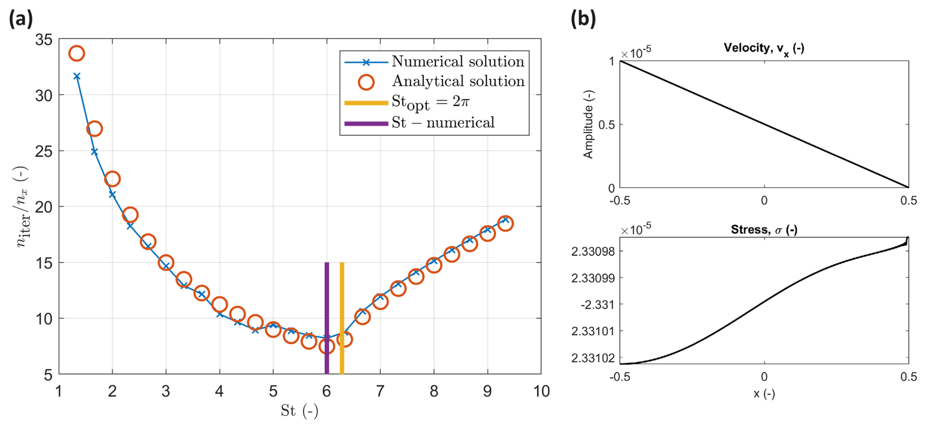
Figure 1 (a) Convergence rate in a homogeneous elastic medium: numerical and analytical results as a function of the dimensionless parameter St. (b) Numerical results of the APT method for velocity and stress fields in the homogeneous medium for the damping scheme (Eq. 5). The upper panel corresponds to the velocity field, and the lower panel shows the stress field.

2.5.2 Numerical experiment 2: effective properties of a homogeneous medium

Let us consider a 1D numerical domain with L_x=1, which is discretized into n_x=1000 grid cells. The material parameters are $K=G=\mathrm{1}$ and Δt=1. For this experiment, velocity boundary conditions are applied by prescribing $v_x(n=\mathrm{1})=\mathrm{1}$ and $v_x(n=n_x)=\mathrm{0}$, where n is a grid cell number in a 1D domain ($v_x(n=\mathrm{1})=\mathrm{1}$ means the velocity v_x=1 at the first grid cell (n=1), which corresponds to the left corner of the 1D domain L_x). All other parameters and initial conditions are set to zero.

Figure 1b shows the velocity field (panel a) and the amplitudes of the stress field. Since the medium is homogeneous, the effective elastic parameters can be calculated exactly: $H_{\mathrm{an}}^{*}=K+\mathrm{4}/\mathrm{3}G=\mathrm{7}/\mathrm{3}$. Numerically, the effective elastic parameters are calculated from the discrete values for the APT method:

$$\begin{array}{}\text{(21)}& H_{\mathrm{num}}^{*}={\displaystyle \frac{{\sum }_{i=\mathrm{1}}^{nx}[{\mathit{\sigma }}_{xx}{]}_i}{{\sum }_{i=\mathrm{1}}^{nx}[\partial u_x/\partial x{]}_i}},\end{array}$$

where u_x=v_xΔt. After 5 n_x iterations in pseudo-time we can report the accuracy (in residuals) as $\mathrm{d}{v}_x={\mathrm{10}}^{-\mathrm{13}}$. This result corresponds to the difference between the numerical value for H^* and the analytical value for $H_{\mathrm{an}}^{*}=\mathrm{7}/\mathrm{3}$ via $(H_{\mathrm{an}}^{*}-H_{\mathrm{num}}^{*})/H_{\mathrm{an}}^{*}\times \mathrm{100}\mathit{\%}$ to as 10⁻¹² %.

2.5.3 Numerical experiment 3: convergence rate in a heterogeneous medium

Let us again consider a 1D numerical domain with L_x=1, which is discretized into n_x=1000 grid cells. The boundary conditions are the same as in the previous section (numerical experiment 2). Now, we consider a heterogeneous medium in 1D represented by layers of different elastic properties. There are 10 layers with the properties $K_{\mathrm{1}}=G_{\mathrm{1}}=\mathrm{1}$ and $K_{\mathrm{2}}=G_{\mathrm{2}}=\mathrm{0.05}$. Figure 2 shows numerical results for the system in Eq. (6). The numerical results correspond to the solution as a function of St until the update of the pseudo-time derivatives becomes within the range 10⁻⁹. It can be seen that the optimal value of St that is valid in a homogeneous medium is not valid here for a heterogeneous medium. Instead, a special scaling is needed of St with a parameter A which is defined below.

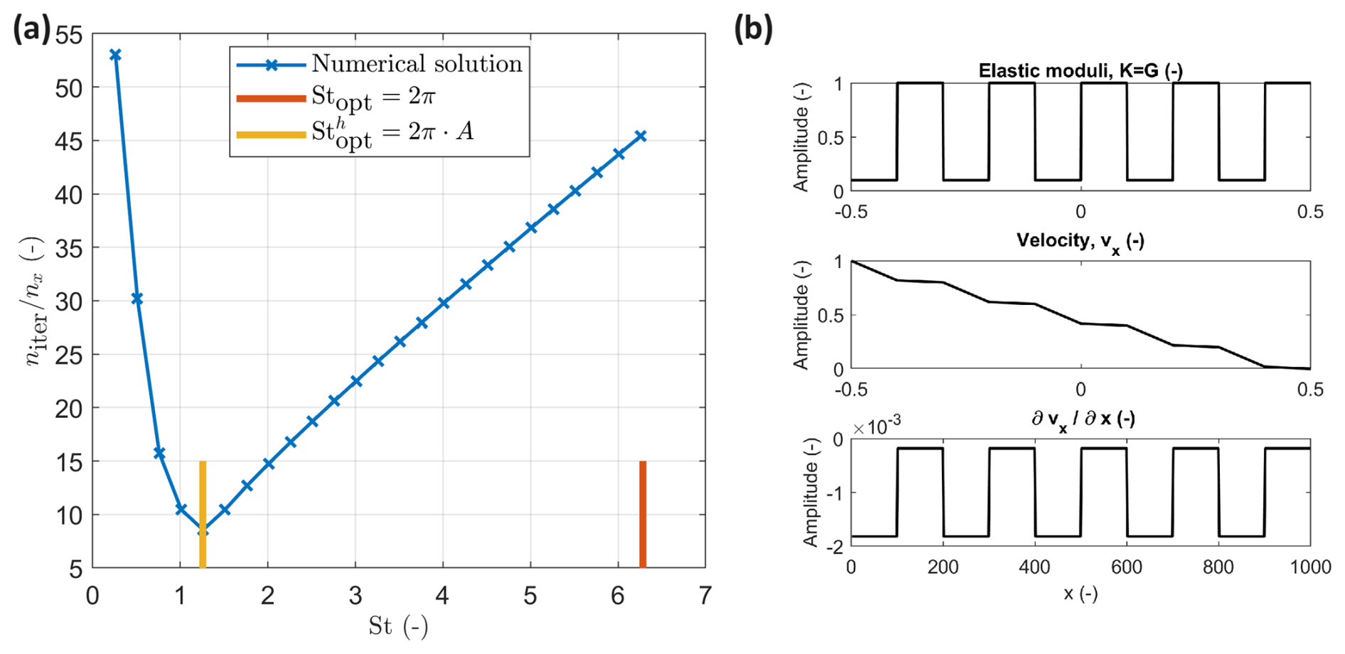
Figure 2 (a) Numerical results: convergence rate in a heterogeneous medium as a function of St. (b) Numerical results for velocity and stress fields in a layered (heterogeneous) medium. The upper panel corresponds to variations of the bulk modulus K (the same as variations in the shear modulus G). The lower panel shows the spatial derivative of the velocity field.

2.5.4 Numerical experiment 4: effective properties of a heterogeneous medium

We perform the numerical experiment considering the damping scheme in Eq. (6) as a function of St. By running a set of numerical simulations with different optimal parameters, we found that the following re-scaling of St_opt via parameter A provides the best fast convergence rate:

$$\begin{array}{}\text{(22)}& {\mathit{St}}_{\text{opt}}^h=A\cdot {\mathit{St}}_{\text{opt}},\end{array}$$

where A is a minimum of the elastic moduli of the softest material divided by volume fraction of the weakest phase ϕ,

$$\begin{array}{}\text{(23)}& A=min(K_{\mathrm{2}},G_{\mathrm{2}})/\mathit{\varphi }.\end{array}$$

Figure 2 shows the distribution of elastic moduli (panel a), the velocity field, and the spatial derivative of the velocity field. After 5 n_x iterations in pseudo-time, we report the following accuracy (in residuals): $\mathrm{d}{v}_x={\mathrm{10}}^{-\mathrm{7}}$. This result corresponds to the difference between the numerical value for H^* and the analytical value for $H_{\mathrm{an}}^{*}=\mathrm{0.42}\left(\mathrm{42}\right)$ via $(H_{\mathrm{an}}^{*}-H_{\mathrm{num}}^{*})/H_{\mathrm{an}}^{*}\times \mathrm{100}\mathit{\%}$ to $\mathrm{2}\times {\mathrm{10}}^{-\mathrm{3}}\mathit{\%}$ for the damping scheme represented by Eq. (6).

3 Mathematical formulation: viscoelasticity

Now, let us consider viscoelastic equations. The general form is the following:

$$\begin{array}{}\text{(24)}& \left\{\begin{array}{l}\frac{\mathrm{1}}{K}\frac{\partial p}{\partial t}=-\mathrm{\nabla }\cdot \mathbf{v}\\ \frac{\mathrm{1}}{\mathrm{2}G}\frac{\partial \mathit{\tau }}{\partial t}+\frac{\mathit{\tau }}{\mathrm{2}{\mathit{\mu }}_{\mathrm{s}}}=\mathit{\epsilon }-\frac{\mathrm{1}}{\mathrm{3}}(\mathrm{\nabla }\cdot \mathbf{v}){\mathbf{I}}_{\mathrm{2}}\\ \mathrm{0}=\mathrm{\nabla }\cdot (-p{\mathbf{I}}_{\mathrm{2}}+\mathit{\tau }),\end{array}\right.\end{array}$$

where μ_s is the shear viscosity of the solid material, p is the pressure, and τ is the deviatoric stress tensor ($\mathit{\sigma }=-p{\mathbf{I}}_{\mathrm{2}}+\mathit{\tau }$. The system in Eq. (24) can be rewritten for the calculation of effective viscoelastic properties in 1D as

$$\begin{array}{}\text{(25)}& \left\{\begin{array}{l}\frac{\mathrm{1}}{K}\frac{\partial p}{\partial t}=-\frac{\partial v_x}{\partial x}\\ \frac{\mathrm{1}}{\mathrm{2}G}\frac{\partial {\mathit{\tau }}_{xx}}{\partial t}+\frac{{\mathit{\tau }}_{xx}}{\mathrm{2}{\mathit{\mu }}_{\mathrm{s}}}=\left(\frac{\partial v_x}{\partial x}-\frac{\mathrm{1}}{\mathrm{3}}\frac{\partial v_x}{\partial x}\right)\\ \mathrm{0}=\frac{\partial (-p+{\mathit{\tau }}_{xx})}{\partial x},\end{array}.\right.\end{array}$$

3.1 APT scheme for viscoelastic equations

The advantage of this naive APT scheme is that there are minimal modifications to the original formulation of the APT method for elasticity equations presented in the previous sections. The system in Eq. (25) can be rewritten as APT scheme 2:

$$\begin{array}{}\text{(26)}& \left\{\begin{array}{l}\frac{\mathrm{1}}{\stackrel{\mathrm{̃}}{K}}\frac{\partial p}{\partial \stackrel{\mathrm{̃}}{t}}+\frac{\mathrm{1}}{K}\frac{p-\widehat{p}}{\mathrm{\Delta }t}=-\frac{\partial v_x}{\partial x}\\ \frac{\mathrm{1}}{\mathrm{2}\stackrel{\mathrm{̃}}{G}}\frac{\partial {\mathit{\tau }}_{xx}}{\partial \stackrel{\mathrm{̃}}{t}}+\frac{\mathrm{1}}{\mathrm{2}G}\frac{{\mathit{\tau }}_{xx}-{\widehat{\mathit{\tau }}}_{xx}}{\mathrm{\Delta }t}+\frac{{\mathit{\tau }}_{xx}}{\mathrm{2}{\mathit{\mu }}_{\mathrm{s}}}=\left(\frac{\partial v_x}{\partial x}-\frac{\mathrm{1}}{\mathrm{3}}\frac{\partial v_x}{\partial x}\right)\\ \stackrel{\mathrm{̃}}{\mathit{\rho }}\frac{\partial v_x}{\partial \stackrel{\mathrm{̃}}{t}}=-\frac{\partial {\mathit{\sigma }}_{xx}}{\partial x},\end{array}\right.\end{array}$$

where

$$\begin{array}{}\text{(27)}& {\displaystyle \frac{\mathrm{\Delta }\stackrel{\mathrm{̃}}{t}}{\stackrel{\mathrm{̃}}{\mathit{\rho }}}}={\displaystyle \frac{{\stackrel{\mathrm{̃}}{V}}_{\mathrm{p}}\mathrm{\Delta }\stackrel{\mathrm{̃}}{t}{L}_x}{\mathit{St}{H}^{\mathrm{ve}}}},\end{array}$$

and ${\stackrel{\mathrm{̃}}{H}}^{\mathrm{ve}}$ is defined as

$$\begin{array}{}\text{(28)}& H^{\mathrm{ve}}={\left((K\mathrm{\Delta }t+{\displaystyle \frac{\mathrm{4}}{\mathrm{3}}}{G}^{\mathrm{ve}})\right)}^{-\mathrm{1}},\end{array}$$

where

$$\begin{array}{}\text{(29)}& G^{\mathrm{ve}}={\left({\displaystyle \frac{\mathrm{1}}{{\mathit{\mu }}_{\mathrm{s}}}}+{\displaystyle \frac{\mathrm{1}}{G\mathrm{\Delta }t}}\right)}^{-\mathrm{1}}\end{array}$$

is the apparent “viscoelastic” shear modulus. Let us modify the scheme (Eq. 26) by re-arranging terms and omitting quantities that are constant during the iterations over $\stackrel{\mathrm{̃}}{t}$:

$$\begin{array}{}\text{(30)}& \left\{\begin{array}{l}\frac{\mathrm{1}}{\stackrel{\mathrm{̃}}{K}}\frac{\partial p}{\partial \stackrel{\mathrm{̃}}{t}}+\frac{\mathrm{1}}{K}\frac{p}{\mathrm{\Delta }t}=-\frac{\partial v_x}{\partial x}\\ \frac{\mathrm{1}}{\mathrm{2}\stackrel{\mathrm{̃}}{G}}\frac{\partial {\mathit{\tau }}_{xx}}{\partial \stackrel{\mathrm{̃}}{t}}+\frac{{\mathit{\tau }}_{xx}}{\mathrm{2}}\left(\frac{\mathrm{1}}{G\mathrm{\Delta }t}+\frac{\mathrm{1}}{{\mathit{\mu }}_{\mathrm{s}}}\right)=\left(\frac{\partial v_x}{\partial x}-\frac{\mathrm{1}}{\mathrm{3}}\frac{\partial v_x}{\partial x}\right)\\ \stackrel{\mathrm{̃}}{\mathit{\rho }}\frac{\partial v_x}{\partial \stackrel{\mathrm{̃}}{t}}=-\frac{\partial {\mathit{\sigma }}_{xx}}{\partial x}.\end{array}\right.\end{array}$$

Further simplifications leads to the following system:

$$\begin{array}{}\text{(31)}& \left\{\begin{array}{l}\frac{\mathrm{1}}{\stackrel{\mathrm{̃}}{K}}\frac{\partial p}{\partial \stackrel{\mathrm{̃}}{t}}+\frac{\mathrm{1}}{K}\frac{p}{\mathrm{\Delta }t}=-\frac{\partial v_x}{\partial x}\\ \frac{\mathrm{1}}{\mathrm{2}\stackrel{\mathrm{̃}}{G}}\frac{\partial {\mathit{\tau }}_{xx}}{\partial \stackrel{\mathrm{̃}}{t}}+\frac{{\mathit{\tau }}_{xx}}{\mathrm{2}}\frac{\mathrm{1}}{G^{\text{ve}}}=\left(\frac{\partial v_x}{\partial x}-\frac{\mathrm{1}}{\mathrm{3}}\frac{\partial v_x}{\partial x}\right)\\ \stackrel{\mathrm{̃}}{\mathit{\rho }}\frac{\partial v_x}{\partial \stackrel{\mathrm{̃}}{t}}=-\frac{\partial {\mathit{\sigma }}_{xx}}{\partial x}\end{array}.\right.\end{array}$$

Note that (e.g., assuming G^ve=G) the present system in Eq. (31) becomes identical to the system in Eq. (B4) (or 6), which corresponds to the elasticity equations. Therefore, all the analyses presented for elasticity equations in the previous sections can be applied to the viscoelastic equations. If $K=G^{\text{ve}}=\mathrm{1}$, then

$$\begin{array}{}\text{(32)}& {\mathit{St}}_{\text{opt}}=\mathrm{2}\mathit{\pi },\end{array}$$

which is the same value as in the case of the elasticity equations. It can be seen that the analytical and numerical results are in excellent agreement (Fig. 3), which validates the proposed approach.

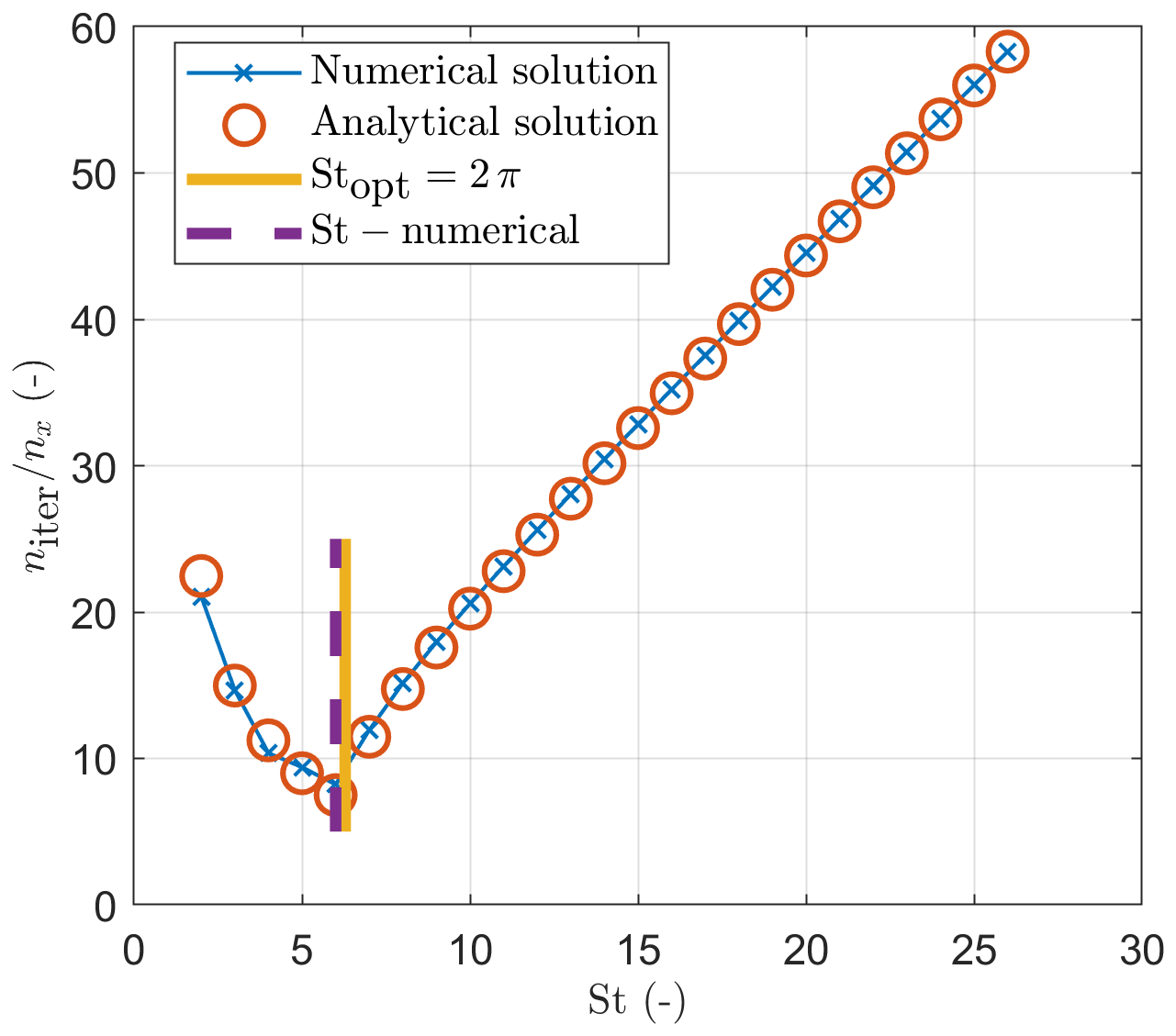
Figure 3 Convergence rate in a homogeneous viscoelastic medium: numerical and analytical results as a function of the dimensionless parameter St.

4 Mathematical formulation: coupled hydromechanics–quasi-static poroelasticity

The first-order velocity–stress system of Biot's equations in 1D can be written as (Biot, 1962)

$$\begin{array}{}\text{(33)}& {\displaystyle }\left(\begin{array}{c}\frac{\partial \stackrel{\mathrm{‾}}{p}}{\partial t}\\ \frac{\partial p_{\mathrm{f}}}{\partial t}\end{array}\right)=-K_{\mathrm{u}}\left(\begin{array}{cc}\mathrm{1}& B\\ B& \frac{B}{\mathit{\alpha }}\end{array}\right)\left(\begin{array}{c}\frac{\partial v_x^{\mathrm{s}}}{\partial x}\\ \frac{\partial q_x^{\mathrm{D}}}{\partial x}\end{array}\right),\text{(34)}& {\displaystyle \frac{\partial {\stackrel{\mathrm{‾}}{\mathit{\tau }}}_{xx}}{\partial t}}=\mathrm{2}{G}_{\mathrm{u}}\left({\displaystyle \frac{\partial v_x}{\partial x}}-{\displaystyle \frac{\mathrm{1}}{\mathrm{3}}}{\displaystyle \frac{\partial v_x}{\partial x}}\right),\end{array}$$

and

$$\begin{array}{}\text{(35)}& \left(\begin{array}{c}\mathrm{0}\\ \mathrm{0}\end{array}\right)=\left(\begin{array}{c}\frac{\partial (-p+{\mathit{\tau }}_{xx})}{\partial x}\\ \frac{{\mathit{\eta }}_{\mathrm{f}}}{k}{q}_x^{\mathrm{D}}+\frac{\partial p_{\mathrm{f}}}{\partial x}\end{array}\right).\end{array}$$

Table 1 List of symbols.

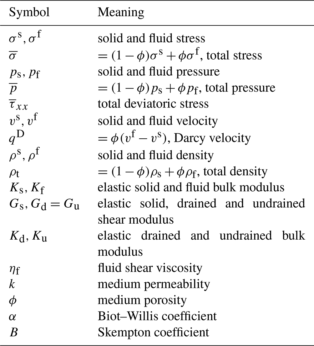
The list of symbols is given in Table 1. From the general principles of thermodynamics, the matrices of coefficients in the expression in Eq. (33) must be positive-definite. For simplicity, the expressions in Eqs. (33) and (34) can be combined, leading to

$$\begin{array}{}\text{(36)}& \left(\begin{array}{c}\frac{\partial {\stackrel{\mathrm{‾}}{\mathit{\sigma }}}_{xx}}{\partial t}\\ -\frac{\partial p_{\mathrm{f}}}{\partial t}\end{array}\right)=\left(\begin{array}{cc}{K}_{\mathrm{u}}+\frac{\mathrm{4}}{\mathrm{3}}{G}_{\mathrm{u}}& K_{\mathrm{u}}B\\ K_{\mathrm{u}}B& \frac{K_{\mathrm{u}}B}{\mathit{\alpha }}\end{array}\right)\left(\begin{array}{c}\frac{\partial v_x^{\mathrm{s}}}{\partial x}\\ \frac{\partial q_x^{\mathrm{D}}}{\partial x}\end{array}\right),\end{array}$$

where ${\stackrel{\mathrm{‾}}{\mathit{\sigma }}}_{xx}=-\stackrel{\mathrm{‾}}{p}+{\stackrel{\mathrm{‾}}{\mathit{\tau }}}_{xx}$. For an isotropic material saturated with a single fluid, in which the solid frame consists of a single isotropic mineral, the Biot–Willis coefficient is

$$\begin{array}{}\text{(37)}& \mathit{\alpha }=\mathrm{1}-{\displaystyle \frac{K_{\mathrm{d}}}{K_{\mathrm{s}}}},\end{array}$$

and the Skempton coefficient, B, is

$$\begin{array}{}\text{(38)}& B={\displaystyle \frac{\mathrm{1}/K_{\mathrm{d}}-\mathrm{1}/K_{\mathrm{s}}}{\mathrm{1}/K_{\mathrm{d}}-\mathrm{1}/K_{\mathrm{s}}+\mathit{\varphi }(\mathrm{1}/K_{\mathrm{f}}-\mathrm{1}/K_{\mathrm{s}})}}.\end{array}$$

Other useful parameters include the undrained bulk modulus, K_u,

$$\begin{array}{}\text{(39)}& K_{\mathrm{u}}=K_{\mathrm{d}}{\left(\mathrm{1}-\mathit{\alpha }B\right)}^{-\mathrm{1}}\equiv K_{\mathrm{d}}+{\mathit{\alpha }}^{\mathrm{2}}M,\end{array}$$

and the fluid storage coefficient, M,

$$\begin{array}{}\text{(40)}& M=K_{\mathrm{u}}B/\mathit{\alpha }.\end{array}$$

Equation (39) is known as Gassmann's equation for fluid-saturated bulk modulus (Gassmann, 1951; Alkhimenkov, 2023).

4.1 APT method for the quasi-static Biot poroelastic equations

Let us write the APT method for the quasi-static Biot poroelastic equations expressed as Eqs. (33)–(35):

$$\begin{array}{}\text{(41)}& \left(\begin{array}{c}\frac{\mathrm{1}}{{\stackrel{\mathrm{̃}}{K}}_{\mathrm{1}}}\frac{\partial \stackrel{\mathrm{‾}}{p}}{\partial \stackrel{\mathrm{̃}}{t}}\\ \frac{\mathrm{1}}{{\stackrel{\mathrm{̃}}{K}}_{\mathrm{2}}}\frac{\partial p_{\mathrm{f}}}{\partial \stackrel{\mathrm{̃}}{t}}\end{array}\right)+{\displaystyle \frac{\mathrm{1}}{K_{\mathrm{u}}}}\left(\begin{array}{c}\frac{\stackrel{\mathrm{‾}}{p}-\widehat{\stackrel{\mathrm{‾}}{p}}}{\mathrm{\Delta }t}\\ \frac{p_{\mathrm{f}}-{\widehat{p}}_{\mathrm{f}}}{\mathrm{\Delta }t}\end{array}\right)=-\left(\begin{array}{cc}\mathrm{1}& B\\ B& \frac{B}{\mathit{\alpha }}\end{array}\right)\left(\begin{array}{c}\frac{\partial v^{\mathrm{s}}}{\partial x}\\ \frac{\partial q^{\mathrm{D}}}{\partial x}\end{array}\right),\end{array}$$

where $\widehat{\stackrel{\mathrm{‾}}{p}}$ and ${\widehat{p}}_{\mathrm{f}}$ are the total and fluid pressures at the previous physical time step, ${\stackrel{\mathrm{̃}}{K}}_{\mathrm{1}}=K_{\mathrm{u}}$. For the total deviatoric stress the corresponding equation is

$$\begin{array}{}\text{(42)}& {\displaystyle \frac{\mathrm{1}}{\mathrm{2}{\stackrel{\mathrm{̃}}{G}}_{\mathrm{1}}}}{\displaystyle \frac{\partial {\stackrel{\mathrm{‾}}{\mathit{\tau }}}_{xx}}{\partial \stackrel{\mathrm{̃}}{t}}}+{\displaystyle \frac{\mathrm{1}}{\mathrm{2}{G}_{\mathrm{u}}}}{\displaystyle \frac{{\stackrel{\mathrm{‾}}{\mathit{\tau }}}_{xx}-{\widehat{\stackrel{\mathrm{‾}}{\mathit{\tau }}}}_{xx}}{\mathrm{\Delta }t}}=\left({\displaystyle \frac{\partial v_x}{\partial x}}-{\displaystyle \frac{\mathrm{1}}{\mathrm{3}}}{\displaystyle \frac{\partial v_x}{\partial x}}\right),\end{array}$$

where ${\widehat{\stackrel{\mathrm{‾}}{\mathit{\tau }}}}_{xx}$ is the total stress deviator at the previous physical time step and ${\stackrel{\mathrm{̃}}{G}}_{\mathrm{1}}=G_{\mathrm{u}}$ . The system in Eq. (35) is rewritten as

$$\begin{array}{}\text{(43)}& \left(\begin{array}{cc}{\stackrel{\mathrm{̃}}{\mathit{\rho }}}_{\mathrm{t}}& \mathrm{0}\\ \mathrm{0}& {\stackrel{\mathrm{̃}}{\mathit{\rho }}}_{\mathrm{a}}\end{array}\right)\left(\begin{array}{c}\frac{\partial v_i^{\mathrm{s}}}{\partial \stackrel{\mathrm{̃}}{t}}\\ -\frac{\partial q_i^{\mathrm{D}}}{\partial \stackrel{\mathrm{̃}}{t}}\end{array}\right)=\left(\begin{array}{c}\frac{\partial (-p+{\mathit{\tau }}_{xx})}{\partial x}\\ \frac{{\mathit{\eta }}_{\mathrm{f}}}{k}{q}_i^{\mathrm{D}}+\frac{\partial p_{\mathrm{f}}}{\partial x}\end{array}\right),\end{array}$$

where ${\stackrel{\mathrm{̃}}{\mathit{\rho }}}_{\mathrm{t}}$ and ${\stackrel{\mathrm{̃}}{\mathit{\rho }}}_{\mathrm{a}}$ are to-be-determined numerical parameters. A discrete form of the system in Eqs. (41)–(43) is presented in Appendix F. In summary, we need the following combinations of the numerical parameters to effectively solve the system in Eqs. (41)–(43): ${\stackrel{\mathrm{̃}}{K}}_{\mathrm{1}}\mathrm{\Delta }\stackrel{\mathrm{̃}}{t}$, ${\stackrel{\mathrm{̃}}{K}}_{\mathrm{2}}\mathrm{\Delta }\stackrel{\mathrm{̃}}{t}$, ${\stackrel{\mathrm{̃}}{G}}_{\mathrm{u}}\mathrm{\Delta }\stackrel{\mathrm{̃}}{t}$, $\mathrm{\Delta }\stackrel{\mathrm{̃}}{t}/{\stackrel{\mathrm{̃}}{\mathit{\rho }}}_{\mathrm{t}}$, and $\mathrm{\Delta }\stackrel{\mathrm{̃}}{t}/{\stackrel{\mathrm{̃}}{\mathit{\rho }}}_{\mathrm{a}}$. A dispersion analysis of Eqs. (41)–(43) leads to the system of five equations. Without the loss of generality, we analyze the APT method of the expressions in Eqs. (36) and (35), which corresponds to the system of four equations in the dispersion analysis.

The numerical primary or P-wave velocity of the system in Eqs. (41)–(43) varies as a function of I₂, which is a nondimensional parameter:

$$\begin{array}{}\text{(44)}& I_{\mathrm{2}}={\displaystyle \frac{{\mathit{\eta }}_{\mathrm{f}}}{k}}{\stackrel{\mathrm{̃}}{\mathit{\rho }}}_{\mathrm{a}}{\mathit{\tau }}^{*},\end{array}$$

where τ^* is a characteristic time. The physical meaning of I₂ is the following: I₂ controls the behavior of Biot's slow wave; if $I_{\mathrm{2}}>>>\mathrm{1}$ the slow wave behaves as a propagating wave, and if $I_{\mathrm{2}}<<<\mathrm{1}$ the slow wave behaves as a diffusive mode. For details on the nondimensional analysis of these equations we refer to Alkhimenkov et al. (2021b). The CFL condition for the system in Eqs. (41)–(43) suggests that (Alkhimenkov et al., 2021a)

$$\begin{array}{}\text{(45)}& \mathrm{\Delta }\stackrel{\mathrm{̃}}{t}\le {\displaystyle \frac{\mathrm{\Delta }x}{{\stackrel{\mathrm{̃}}{V}}_{\mathrm{p}}^{\mathrm{HF}}}}\text{or}\mathrm{\Delta }\stackrel{\mathrm{̃}}{t}={\displaystyle \frac{\stackrel{\mathrm{̃}}{C}\mathrm{\Delta }x}{{\stackrel{\mathrm{̃}}{V}}_{\mathrm{p}}^{\mathrm{HF}}}},\end{array}$$

where ${\stackrel{\mathrm{̃}}{V}}_{\mathrm{p}}^{\mathrm{HF}}$ is the numerical P-wave velocity at high frequencies and $\stackrel{\mathrm{̃}}{C}\le \mathrm{1}$. Note that ${\stackrel{\mathrm{̃}}{V}}_{\mathrm{p}}^{\mathrm{HF}}>{\stackrel{\mathrm{̃}}{V}}_{\mathrm{p}}^{\mathrm{LF}}$, where the latter is the numerical P-wave velocity at low frequencies. Since the exact expression for ${\stackrel{\mathrm{̃}}{V}}_{\mathrm{p}}^{\mathrm{HF}}$ is cumbersome, we can modify the CFL condition in Eq. (45) as

$$\begin{array}{}\text{(46)}& \mathrm{\Delta }\stackrel{\mathrm{̃}}{t}={\displaystyle \frac{\stackrel{\mathrm{̃}}{C}\mathrm{\Delta }x}{{\stackrel{\mathrm{̃}}{V}}_{\mathrm{p}}^{\mathrm{LF}}}},\end{array}$$

where

$$\begin{array}{}\text{(47)}& {\stackrel{\mathrm{̃}}{V}}_{\mathrm{p}}^{\mathrm{LF}}=\sqrt{{\displaystyle \frac{{\stackrel{\mathrm{̃}}{K}}_{\mathrm{1}}+\frac{\mathrm{4}}{\mathrm{3}}{\stackrel{\mathrm{̃}}{G}}_{\mathrm{1}}}{\stackrel{\mathrm{̃}}{\mathit{\rho }}}}}=\sqrt{{\displaystyle \frac{K_{\mathrm{u}}+\frac{\mathrm{4}}{\mathrm{3}}{G}_{\mathrm{u}}}{\stackrel{\mathrm{̃}}{\mathit{\rho }}}}}=\sqrt{{\displaystyle \frac{H_{\mathrm{u}}}{\stackrel{\mathrm{̃}}{\mathit{\rho }}}}},\end{array}$$

where $H_{\mathrm{u}}=K_{\mathrm{u}}+\frac{\mathrm{4}}{\mathrm{3}}{G}_{\mathrm{u}}$ is the undrained P-wave modulus. The reason for setting ${\stackrel{\mathrm{̃}}{K}}_{\mathrm{1}}=K_{\mathrm{u}}$ and ${\stackrel{\mathrm{̃}}{G}}_{\mathrm{1}}=G$ is simplicity; since the fourth-order equation has only two degrees of freedom for the APT method's parameter choices, a different choice of these parameters would simply re-scale the two final optimal parameters.

4.1.1 The choice of the numerical parameters

The analysis here is similar to that for a single-phase medium. From the stability analysis (Eq. 46), we determine that

$$\begin{array}{}\text{(48)}& {\stackrel{\mathrm{̃}}{V}}_{\mathrm{p}}^{\mathrm{LF}}\mathrm{\Delta }\stackrel{\mathrm{̃}}{t}=\stackrel{\mathrm{̃}}{C}\mathrm{\Delta }x.\end{array}$$

Let us introduce a dimensionless parameter, the Strouhal number (St), which is expressed as

$$\begin{array}{}\text{(49)}& \mathit{St}={\displaystyle \frac{L_x}{{\stackrel{\mathrm{̃}}{V}}_{\mathrm{p}}^{\mathrm{LF}}\mathrm{\Delta }t}}.\end{array}$$

By analogy with the expression in Eq. (17), we write the formula for the first numerical combination:

$$\begin{array}{}\text{(50)}& {\displaystyle \frac{\mathrm{\Delta }\stackrel{\mathrm{̃}}{t}}{{\stackrel{\mathrm{̃}}{\mathit{\rho }}}_{\mathrm{t}}}}={\displaystyle \frac{{\stackrel{\mathrm{̃}}{V}}_{\mathrm{p}}^{\mathrm{LF}}\mathrm{\Delta }\stackrel{\mathrm{̃}}{t}{L}_x}{\mathit{St}{H}_{\mathrm{u}}\mathrm{\Delta }t}}.\end{array}$$

The second numerical combination is

$$\begin{array}{}\text{(51)}& {\stackrel{\mathrm{̃}}{G}}_{\mathrm{1}}\mathrm{\Delta }\stackrel{\mathrm{̃}}{t}={\displaystyle \frac{({\stackrel{\mathrm{̃}}{V}}_{\mathrm{p}}^{\mathrm{LF}}\mathrm{\Delta }\stackrel{\mathrm{̃}}{t}{)}^{\mathrm{2}}}{(r+\frac{\mathrm{4}}{\mathrm{3}})}}{\left({\displaystyle \frac{\mathrm{\Delta }\stackrel{\mathrm{̃}}{t}}{{\stackrel{\mathrm{̃}}{\mathit{\rho }}}_{\mathrm{t}}}}\right)}^{-\mathrm{1}},\end{array}$$

where $r=K_{\mathrm{u}}/G_{\mathrm{u}}$. Note that ${\stackrel{\mathrm{̃}}{V}}_{\mathrm{p}}^{\mathrm{LF}}\mathrm{\Delta }\stackrel{\mathrm{̃}}{t}$ and $\mathrm{\Delta }\stackrel{\mathrm{̃}}{t}/{\stackrel{\mathrm{̃}}{\mathit{\rho }}}_{\mathrm{t}}$ are already defined above; therefore, it is straightforward to calculate ${\stackrel{\mathrm{̃}}{G}}_{\mathrm{1}}\mathrm{\Delta }\stackrel{\mathrm{̃}}{t}$. Calculation of ${\stackrel{\mathrm{̃}}{K}}_{\mathrm{1}}\mathrm{\Delta }\stackrel{\mathrm{̃}}{t}$ is also straightforward: ${\stackrel{\mathrm{̃}}{K}}_{\mathrm{1}}\mathrm{\Delta }\stackrel{\mathrm{̃}}{t}=r{\stackrel{\mathrm{̃}}{G}}_{\mathrm{1}}\mathrm{\Delta }\stackrel{\mathrm{̃}}{t}$. The next numerical combination ${\stackrel{\mathrm{̃}}{K}}_{\mathrm{2}}\mathrm{\Delta }\stackrel{\mathrm{̃}}{t}$ is

$$\begin{array}{}\text{(52)}& {\stackrel{\mathrm{̃}}{K}}_{\mathrm{2}}\mathrm{\Delta }\stackrel{\mathrm{̃}}{t}=({\stackrel{\mathrm{̃}}{V}}_{\mathrm{p}}^{\mathrm{LF}}\mathrm{\Delta }\stackrel{\mathrm{̃}}{t}{)}^{\mathrm{2}}{\left({\displaystyle \frac{{\stackrel{\mathrm{̃}}{V}}_{\mathrm{p}}^{\mathrm{LF}}\mathrm{\Delta }\stackrel{\mathrm{̃}}{t}{L}_x}{\mathit{St}{K}_{\mathrm{u}}B/\mathit{\alpha }\mathrm{\Delta }t}}\right)}^{-\mathrm{1}}.\end{array}$$

For the last combination $\mathrm{\Delta }\stackrel{\mathrm{̃}}{t}/{\stackrel{\mathrm{̃}}{\mathit{\rho }}}_{\mathrm{a}}$, we explore the discrete system of equations and find that

$$\begin{array}{}\text{(53)}& {\displaystyle \frac{\mathrm{\Delta }\stackrel{\mathrm{̃}}{t}}{{\stackrel{\mathrm{̃}}{\mathit{\rho }}}_{\mathrm{a}}}}={\displaystyle \frac{\mathrm{\Delta }\stackrel{\mathrm{̃}}{t}}{{\stackrel{\mathrm{̃}}{\mathit{\rho }}}_{\mathrm{t}}}}{\displaystyle \frac{{\mathit{\eta }}_{\mathrm{f}}}{k}}.\end{array}$$

Now, the system in Eqs. (41)–(43) can be solved.

In order to find the optimal values of St, we perform the same dispersion analysis as for a single-phase medium. A solution of traveling waves in dissipative media is

$$\begin{array}{}\text{(54)}& F(\stackrel{\mathrm{̃}}{t},x)=\exp \left[{\displaystyle \frac{(\mathit{\gamma }{\stackrel{\mathrm{̃}}{V}}_{\mathrm{p}}^{\mathrm{LF}}\stackrel{\mathrm{̃}}{t}+\mathit{\pi }\mathit{\omega }xi)}{L_x}}\right].\end{array}$$

A dispersion analysis of the system in Eqs. (36) and (35) leads to a 4×4 amplification matrix. The discriminant of this matrix has four roots. The optimal value of St that corresponds to the fastest attenuation of propagating waves depends on the parameter I₂. Let us consider two end-member scenarios for values of I₂, which are explored in the next section.

4.1.2 Approximation: reduced-order equations

To find the optimal values of optimal parameters for the system in Eqs. (41)–(43) a solution of the fifth-order (or fourth-order) polynomial is required. However, if we neglect the coupling in the stress–strain relation, we arrive at a fourth-order (consider only the fourth-order polynomial for simplicity) polynomial where the roots can be easily separated: two roots are the same as for single-phase elastic media and the other two roots are more complicated and belong to Darcy's law.

Lets us assume a particular value of coupling parameters: B=0, $B/\mathit{\alpha }$, and I₂ as variables (Δx=1). The discriminant D of the matrix amplification matrix that corresponds to the expressions in Eqs. (36) and (35) is (see also the Maple file):

$$\begin{array}{}\text{(55)}& \begin{array}{rl}D& ={\displaystyle \frac{\mathrm{3}}{\mathrm{7}\mathit{St}+\mathrm{3}{I}_{\mathrm{2}}}}\left[\right(\left(\mathrm{7}\mathit{St}\right)/\mathrm{3}+I_{\mathrm{2}}){\mathit{\gamma }}^{\mathrm{2}}\\ & +(\mathrm{7}/\mathrm{3}{\mathit{St}}^{\mathrm{2}}+I_{\mathrm{2}}\mathit{St}B/\mathit{\alpha }+I_{\mathrm{2}})\mathit{\gamma }+B/\mathit{\alpha }\mathit{St}\left(\right(\mathit{\pi }B/\mathit{\alpha }{)}^{\mathrm{2}}+I_{\mathrm{2}}\left)\right]\\ & \times ({\mathit{\pi }}^{\mathrm{2}}+\mathit{St}\mathit{\gamma }+{\mathit{\gamma }}^{\mathrm{2}}).\end{array}\end{array}$$

Setting D=0 and solving for γ, we get four roots. Two of them correspond to the term $({\mathit{\pi }}^{\mathrm{2}}+St\mathit{\gamma }+{\mathit{\gamma }}^{\mathrm{2}})$ and are the same as for single-phase media:

$$\begin{array}{}\text{(56)}& {\displaystyle }{\mathit{\gamma }}_{\mathrm{1}}=-{\displaystyle \frac{\mathit{St}}{\mathrm{2}}}+{\displaystyle \frac{\sqrt{-\mathrm{4}{\mathit{\pi }}^{\mathrm{2}}+{\mathit{St}}^{\mathrm{2}}}}{\mathrm{2}}},\text{(57)}& {\displaystyle }{\mathit{\gamma }}_{\mathrm{2}}=-{\displaystyle \frac{\mathit{St}}{\mathrm{2}}}-{\displaystyle \frac{\sqrt{-\mathrm{4}{\mathit{\pi }}^{\mathrm{2}}+{\mathit{St}}^{\mathrm{2}}}}{\mathrm{2}}}.\end{array}$$

We are interested when the discriminant is zero: $-\mathrm{4}{\mathit{\pi }}^{\mathrm{2}}+{\mathit{St}}^{\mathrm{2}}=\mathrm{0}$. The resulting solution for St has two roots: 2π and −2π. Taking the positive root we get

$$\begin{array}{}\text{(58)}& \mathit{St}={\mathit{St}}_{\text{opt}}=\mathrm{2}\mathit{\pi },\end{array}$$

which is the optimal value of the numerical parameter St that corresponds to the fastest attenuation of propagating waves for $I_{\mathrm{2}}>>>\mathrm{1}$. For $I_{\mathrm{2}}<<<\mathrm{1}$ the corresponding roots are cumbersome (while have an explicit formulation: St_opt=4.11); therefore, we refer an interested reader to the Maple script.

4.2 APT method: general case

Lets us assume a particular value of coupling parameters: $B=\mathrm{5}/\mathrm{8}$ and α=0.5 (which corresponds to $B/\mathit{\alpha }=\mathrm{5}/\mathrm{4}$), and we will vary I₂ from low to high values.

4.2.1 APT method for $I_{\mathrm{2}}>>>\mathrm{1}$

Figure 4a shows the numerical and analytical results for the system in Eqs. (41)–(43) for I₂=1000 (see explanation in Sect. 2.4). The numerical results correspond to the solution with different St numbers until the update of the pseudo-time derivatives becomes less than 10⁻¹¹. The analytical result corresponds to the analytical solution of the dispersion relations as a function of St. It can be seen that the analytical and numerical results are in excellent agreement (Fig. 4a), which validates the proposed approach. Here St_opt is

$$\begin{array}{}\text{(59)}& \mathit{St}={\mathit{St}}_{\text{opt}}\approx \mathrm{2}\mathit{\pi }.\end{array}$$

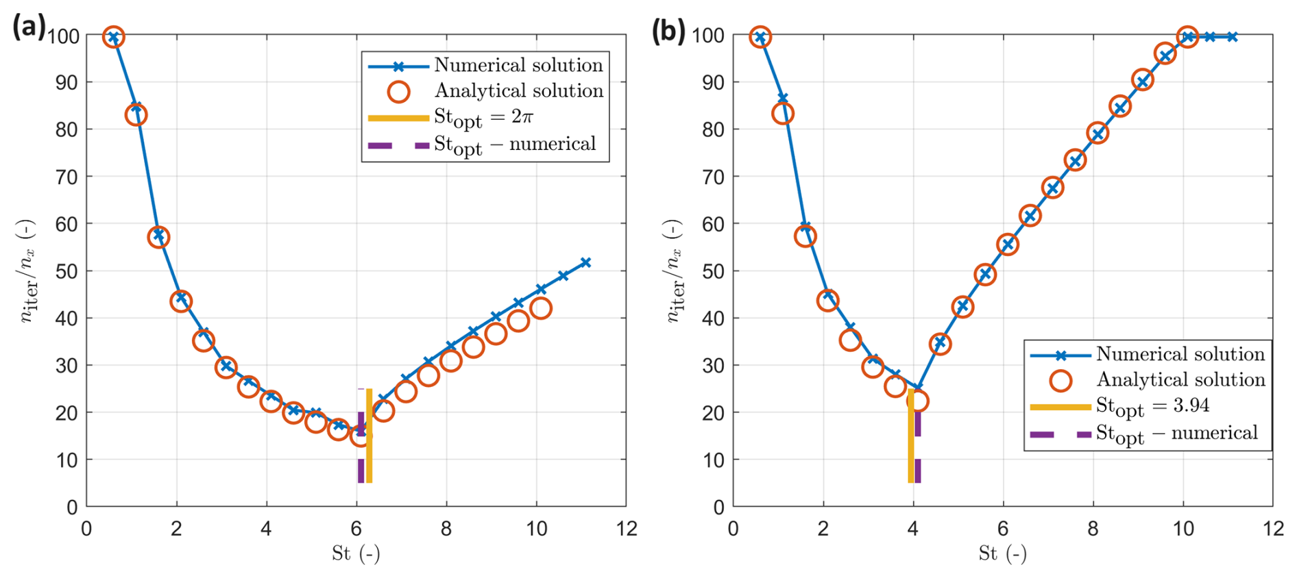
Figure 4 (a) Convergence rate in a homogeneous poroelastic medium for I₂=1000: numerical and analytical results as a function of the dimensionless parameter St. (b) Convergence rate in a homogeneous poroelastic medium for I₂=0.001: numerical and analytical results as a function of the dimensionless parameter St.

4.2.2 APT method for $I_{\mathrm{2}}<<<\mathrm{1}$

Figure 4b shows the numerical and analytical results for the system in Eqs. (41)–(43) for I₂=0.001 (see explanation in Sect. 2.4). The numerical results correspond to the solution with different St numbers until the update of the pseudo-time derivatives (i.e., residual) becomes less than 10⁻¹⁰. The analytical result corresponds to the analytical solution of the dispersion relations as a function of St. It can be seen that the analytical and numerical results are in good agreement (Fig. 4b), which validates the proposed approach. Here St_opt is

$$\begin{array}{}\text{(60)}& \mathit{St}={\mathit{St}}_{\text{opt}}\approx \mathrm{3.94}.\end{array}$$

Figure 5 shows the analytical results for the system in Eqs. (41)–(43) as a function of the dimensionless parameter St and I₂ (by varying ${\mathit{\eta }}_{\mathrm{f}}/k$ only). Note that the optimal value of St depends on the values I₂, B, and $B/\mathit{\alpha }$.

Figure 5 Convergence rate in a homogeneous poroelastic medium as a two-dimensional plot: analytical results as a function of the dimensionless parameters St and I₂. In panel (a) the two white circles correspond to the values of St obtained via expressions in Eqs. (59) and (60). (a) $B=\mathrm{5}/\mathrm{8}$, $B/\mathit{\alpha }=\mathrm{5}/\mathrm{4}$. (b) $B=\mathrm{1}/\mathrm{10}$, $B/\mathit{\alpha }=\mathrm{2}/\mathrm{10}$.

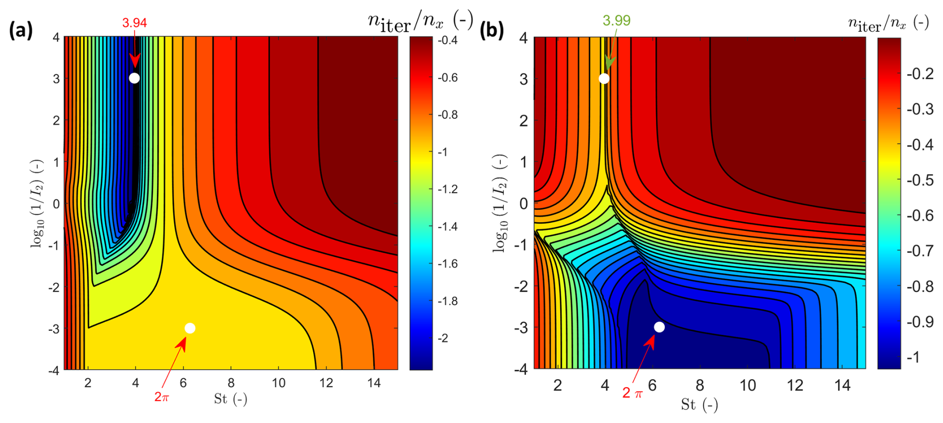
In summary, for practical purposes there is no need to always solve a fourth-order (or fifth-order) polynomial for each set of input parameters of the quasi-static Biot poroelastic equations. In some cases, an average of two parameters can be taken:

$$\begin{array}{}\text{(61)}& \mathit{St}={\mathit{St}}_{\text{opt}}\approx (\mathrm{2}\mathit{\pi }+\mathrm{3.94})/\mathrm{2}\approx \mathrm{5.11}.\end{array}$$

4.2.3 2D numerical simulations: poroelasticity

The accuracy of the proposed St_opt is illustrated numerically in 2D (Fig. 6a–b). It can be seen that the results presented here for 1D need some calibration to be applied to 2D simulations. Note that the numerical parameters are sensitive to boundary and initial conditions, which is explored below. Therefore, some tests must be performed for each numerical setup.

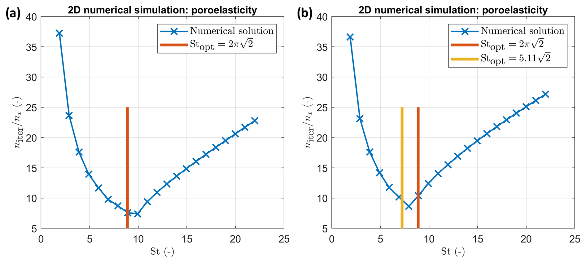
Figure 6 Convergence rate in a homogeneous poroelastic medium for different I₂: numerical result as a function of the dimensionless parameter St. (a) I₂=100. (b) I₂=0.01.

5 Applications: strain localization in poro-elasto-plastic media

The purpose of this section is to demonstrate the applicability of the APT method for ultrahigh-resolution simulations with heterogeneous initial conditions. We address the nonlinear mechanical problem of strain localization in both 2D and 3D contexts, employing an elasto-viscoplastic rheological model. This model is grounded in a hypoelastic-based constitutive framework that accommodates the simulation of large strains. The modeling process follows the formulation of incremental constitutive equations, ensuring the objectivity of the rate fields. In this study, we utilize the Jaumann–Zaremba rate to manage the time-dependent fields.

5.1 Implementation using Graphical Processing Units (GPUs)

The initial code prototyping was conducted on a laptop equipped with a 13th Gen Intel Core i9-13900HX CPU (64 GB RAM) and an NVIDIA GeForce RTX 4090 (16 GB) laptop GPU. For large-scale 3D simulations, the computations were carried out on an NVIDIA DGX-1-like node, featuring 4 NVIDIA Ampere A100 GPUs (each with 80 GB of memory) and an AMD EPYC 7742 server processor with 512 GB of RAM.

5.2 Plasticity implementation

The plasticity model adheres to a consistent poro-elasto-viscoplastic framework, with the yield function defined as

$$\begin{array}{}\text{(62)}& F(\mathit{\tau },p_{\mathrm{e}})=\sqrt{J_{\mathrm{2}}}-A{p}_{\mathrm{e}}-Bc-{\mathit{\eta }}^{\mathrm{vp}}\dot{\mathit{\lambda }},\end{array}$$

where η^vp represents the viscosity of the damper, and $p_{\mathrm{e}}=\stackrel{\mathrm{‾}}{p}-p_{\mathrm{f}}$ is the effective pressure. The yield function specified by Eq. (62) is rate-dependent (Duretz et al., 2019). The plastic potential Q is expressed as

$$\begin{array}{}\text{(63)}& Q(\mathit{\tau },p_{\mathrm{e}})=\sqrt{J_{\mathrm{2}}}-C{p}_{\mathrm{e}}.\end{array}$$

Here, the constants A, B, and C are defined as A=sin (ϕ), B=cos (ϕ), and C=sin (ψ), where ϕ denotes the internal friction angle, and ψ≤ϕ is the dilation angle (with ψ=0 for simplicity in this case).

In the numerical solver, plasticity is implemented through the following steps: (1) compute the components of the trial deviatoric stresses ${\stackrel{\mathrm{‾}}{\mathit{\tau }}}_{ij}^{\mathrm{trial}}$. (2) Using these components, calculate the trial second invariant of the deviatoric stresses, $J_{\mathrm{2}}^{\mathrm{trial}}$. (3) Evaluate F^trial using the expression

$$\begin{array}{}\text{(64)}& F^{\mathrm{trial}}=\sqrt{J_{\mathrm{2}}^{\mathrm{trial}}}-\left(A{p}_{\mathrm{e}}+Bc\right).\end{array}$$

When the material remains in the plastic regime, the components of the trial deviatoric stresses, ${\stackrel{\mathrm{‾}}{\mathit{\tau }}}_{ij}^{\mathrm{trial}}$, are re-scaled according to

$$\begin{array}{}\text{(65)}& {\stackrel{\mathrm{‾}}{\mathit{\tau }}}_{ij}^{\mathrm{new}}={\stackrel{\mathrm{‾}}{\mathit{\tau }}}_{ij}^{\mathrm{trial}}\left(\mathrm{1}-{\displaystyle \frac{F^{\mathrm{trial}}\mathrm{\Delta }t{G}_{\mathrm{u}}}{\sqrt{J_{\mathrm{2}}}(\mathrm{\Delta }t{G}_{\mathrm{u}}+{\mathit{\eta }}^{\mathrm{vp}})}}\right),\end{array}$$

This re-scaling procedure occurs within the pseudo-transient iteration loop, and the process repeats until the components of the updated trial deviatoric stresses, ${\stackrel{\mathrm{‾}}{\mathit{\tau }}}_{ij}^{\mathrm{new}}$, satisfy the condition F^trial=0, and no further re-scaling is needed. This approach is equivalent to the standard formulation involving the plastic multiplier. An interested reader may refer to Alkhimenkov et al. (2024a, b) for more details on the implementation of plasticity.

5.3 2D results: ultrahigh-resolution simulations

Let us consider a 2D numerical domain with $L_x=L_y=\mathrm{1}$. In this set of simulations, pure shear kinematics are imposed at the boundaries of the domain, corresponding to compression along the x axis and extension along the y axis. The model is initialized with pre-stresses of ${\stackrel{\mathrm{‾}}{\mathit{\tau }}}_{xx}=\mathrm{0.0180}$, ${\stackrel{\mathrm{‾}}{\mathit{\tau }}}_{yy}=-\mathrm{0.0180}$, and ${\stackrel{\mathrm{‾}}{\mathit{\tau }}}_{xy}=\mathrm{0}$, while the fluid pressure p_f is set to zero, and the cohesion c is defined as 0.0101. The total pressure in the background material is $\stackrel{\mathrm{‾}}{p}=\mathrm{0.018}$, with a circular anomaly located at the center of the model where the pressure is reduced to $\stackrel{\mathrm{‾}}{p}=\mathrm{0.005}$ (Fig. 7). The radius of this anomaly is $\mathrm{1}/\mathrm{8}$ of the domain size. The simulation is performed over 14 loading increments. The poroelastic properties of the background material are α=0.2958, B=0.0833, G_d=1, K_d=1, and ${\mathit{\eta }}_{\mathrm{f}}/k={\mathrm{10}}^{-\mathrm{2}}$. The porosity, or fluid volume fraction, is ϕ=0.3, and the internal friction angle is φ=30°.

Figure 8 shows the results of the 2D simulation with an ultrahigh resolution of N=10 239² grid cells. The finite thickness of the shear bands confirms that the simulation is mesh-independent as has been shown by Alkhimenkov et al. (2024b). The zoomed-in panels reveal extremely detailed features of the strain localization pattern. The simulation time takes about a few hours.

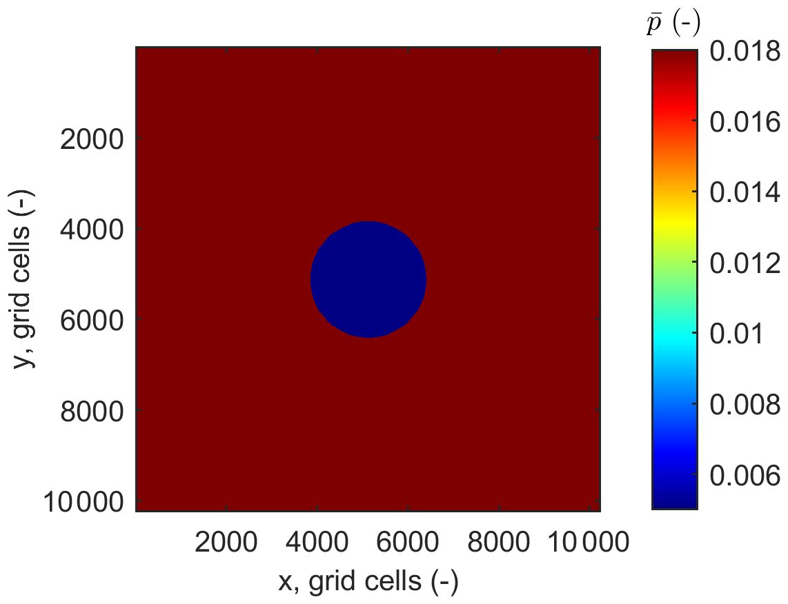
Figure 7 Geometry of the 2D simulation domain: a circular pressure anomaly is located at the center of the model. The resolution is N=10 239² grid cells.

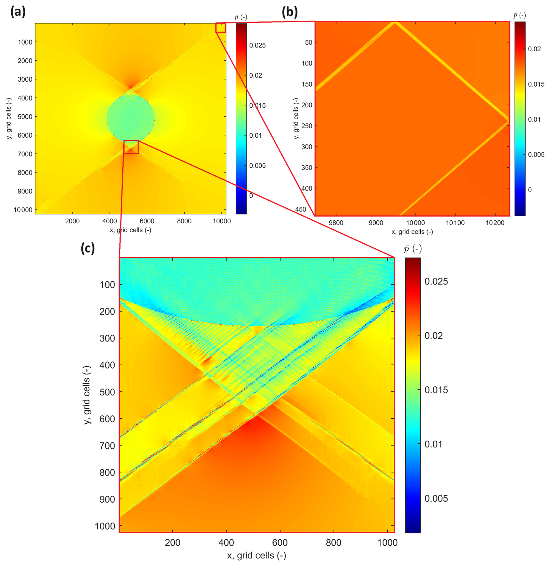
Figure 8 2D simulation results: snapshots of total pressure. Panel (a) shows the full model, while panels (b) and (c) present zoomed-in views of the full model. The resolution is N=10 239² grid cells.

5.4 3D results: ultrahigh-resolution simulations

Let us consider a 3D numerical domain with $L_x=L_y=L_z=\mathrm{1}$. We present 3D results showcasing the spontaneous formation of shear bands under pure shear deformation, initiated by a spherical pressure anomaly (Fig. 9a–b). These 3D simulations further validate the versatility of the APT approach (Fig. 9c–d), demonstrating its robustness in predicting poro-elasto-plastic deformation and capturing brittle failure.

The boundary conditions are defined by compression along the x axis, a slight (1 %) compression along the y axis, and extension along the z axis. The model is initialized with pre-stresses of ${\stackrel{\mathrm{‾}}{\mathit{\tau }}}_{xx}=-\mathrm{0.0098}$, ${\stackrel{\mathrm{‾}}{\mathit{\tau }}}_{yy}=-\mathrm{9.8}\times {\mathrm{10}}^{-\mathrm{05}}$, and ${\stackrel{\mathrm{‾}}{\mathit{\tau }}}_{zz}=\mathrm{0.0098}$, while the shear stress components (${\stackrel{\mathrm{‾}}{\mathit{\tau }}}_{xy}$, ${\stackrel{\mathrm{‾}}{\mathit{\tau }}}_{xz}$, and ${\stackrel{\mathrm{‾}}{\mathit{\tau }}}_{yz}$) are set to zero. The fluid pressure p_f is zero, cohesion c is 0.0101, and the ratio ${\mathit{\eta }}_{\mathrm{f}}/k$ is set at 100. The total pressure in the background material is $\stackrel{\mathrm{‾}}{p}=\mathrm{0}$, with a spherical anomaly located at the center of the model where the pressure is increased to $\stackrel{\mathrm{‾}}{p}=\mathrm{0.005}$. The radius of this anomaly is $\mathrm{1}/\mathrm{8}$ of the domain size. The poroelastic properties of the background material are α=0.2958, B=0.0833, G_d=1, K_d=1, and ${\mathit{\eta }}_{\mathrm{f}}/k={\mathrm{10}}^{\mathrm{2}}$. The porosity is ϕ=0.3, and the internal friction angle is φ=30°. The simulation is conducted over 15 loading increments.

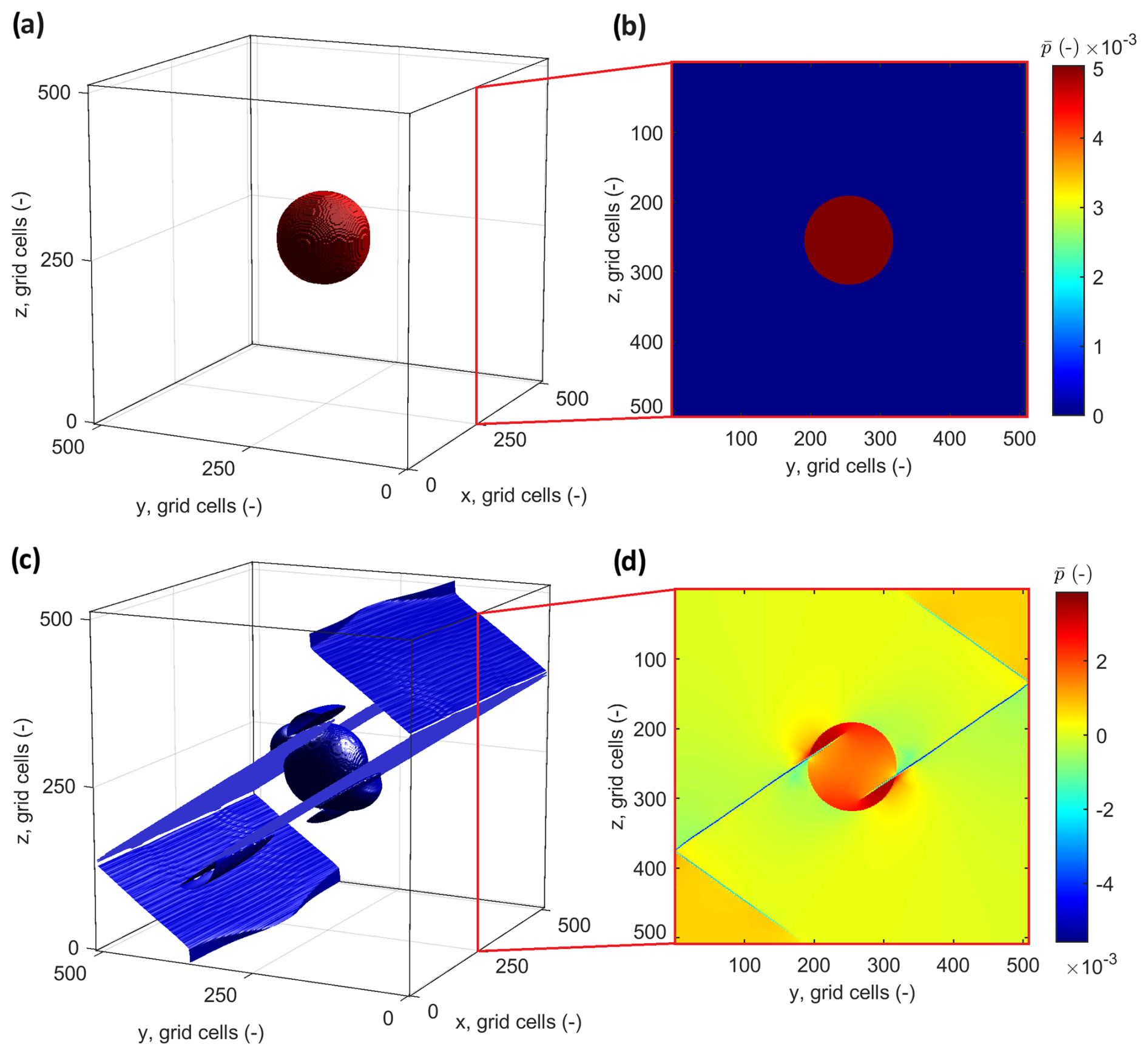
Figure 9 Geometry of the 3D simulation domain: a spherical pressure anomaly is located at the center. Panel (a) corresponds to a 3D view, and panel (b) corresponds to a slice in the y–z plane. Lower panels: 3D simulation results with snapshots of total pressure. Panel (c) shows the 3D view of total pressure. Panel (d) shows the y–z slice of the full 3D model. The resolution is N=512³ grid cells.

6 Discussion

In this section, we analyze the implications of the numerical results presented in the previous sections and establish connections with relevant works in the field. We explore the behavior of the numerical parameters, such as the Strouhal number (St), and their optimal values for different physical models including elastic, viscoelastic, and poroelastic media. Additionally, we assess the influence of dimensionality, initial and boundary conditions, and nonlinearities such as plasticity on the convergence and accuracy of the simulations. This analysis serves as a foundation for further extending these methods to more complex and realistic scenarios.

6.1 Incompressible equations: a connection with the work by Räss et al. (2022)

Räss et al. (2022) performed a comprehensive analysis of the APT method for various problems. However, the work by Räss et al. (2022) was mainly restricted to single-phase media and to incompressible equations. Here we provide connections of the present work to the analysis presented by Räss et al. (2022).

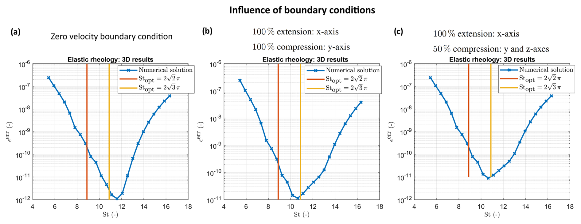
Figure 10 Numerical results in 3D (panels a, b, and c): convergence in an elastic medium as a function of St. The parameter ϵ^err corresponds to the error magnitude of the APT scheme. Simulations in panels (a), (b), and (c) are identical except for the different boundary conditions.

In the present paper we deal with compressible elastic, viscoelastic, or poroelastic equations. As a result, the only numerical parameter that has to be identified is the Strouhal number, St, which is expressed as

$$\begin{array}{}\text{(66)}& \mathit{St}={\displaystyle \frac{f{L}_x}{{\stackrel{\mathrm{̃}}{V}}_{\mathrm{p}}}}={\displaystyle \frac{L_x}{{\stackrel{\mathrm{̃}}{V}}_{\mathrm{p}}\mathrm{\Delta }t}},\end{array}$$

where f is the frequency. However, in the incompressible scenario ($K\to +\mathrm{\infty }$), an additional numerical parameter shows up: $r=\stackrel{\mathrm{̃}}{K}/\stackrel{\mathrm{̃}}{G}$ (which in the compressible case is defined as $r=\stackrel{\mathrm{̃}}{K}/\stackrel{\mathrm{̃}}{G}\equiv K/G$). Räss et al. (2022) discovered that for some specific tasks, the value of r should also be explored as well as the optimal value of St (or, equivalently, Re in their notation). As a result, Räss et al. (2022) reported the optimal values of pairs – r and Re for each set of equations. A connection between the numerical Reynolds number Re (Räss et al., 2022) and the Strouhal number St is provided below.

For the incompressible viscous Stokes equation, Räss et al. (2022) define the numerical Reynolds number, Re, as

$$\begin{array}{}\text{(67)}& \mathit{Re}={\displaystyle \frac{\stackrel{\mathrm{̃}}{\mathit{\rho }}{V}_{\mathrm{p}}^{\mathrm{S}}{L}_x}{{\mathit{\mu }}_{\mathrm{s}}}},\end{array}$$

where $V_{\mathrm{p}}^{\mathrm{S}}$ is the characteristic velocity scale for the incompressible Stokes equations,

$$\begin{array}{}\text{(68)}& V_{\mathrm{p}}^{\mathrm{S}}=\sqrt{{\displaystyle \frac{\stackrel{\mathrm{̃}}{K}+\mathrm{2}\stackrel{\mathrm{̃}}{G}}{\stackrel{\mathrm{̃}}{\mathit{\rho }}}}},\end{array}$$

and μ_s is the shear viscosity. Quantities $\stackrel{\mathrm{̃}}{K}$, $\stackrel{\mathrm{̃}}{G}$, and $\stackrel{\mathrm{̃}}{\mathit{\rho }}$ are the numerical parameters. Note that in the case of incompressible viscoelastic Stokes equations, the quantity μ_s is replaced by μ^ve:

$$\begin{array}{}\text{(69)}& {\mathit{\mu }}^{\mathrm{ve}}={\left({\displaystyle \frac{\mathrm{1}}{G\mathrm{\Delta }t}}+{\displaystyle \frac{\mathrm{1}}{{\mathit{\mu }}_{\mathrm{s}}}}\right)}^{-\mathrm{1}}.\end{array}$$

As a result, for the incompressible viscoelastic Stokes equations, the numerical Reynolds number, Re, is defined as

$$\begin{array}{}\text{(70)}& \mathit{Re}={\displaystyle \frac{\stackrel{\mathrm{̃}}{\mathit{\rho }}{V}_{\mathrm{p}}^{\mathrm{S}}{L}_x}{{\mathit{\mu }}^{\mathrm{ve}}}}.\end{array}$$

In the present paper, from Eq. (27) for viscoelastic media, we can infer the Strouhal number:

$$\begin{array}{}\text{(71)}& \mathit{St}={\displaystyle \frac{\stackrel{\mathrm{̃}}{\mathit{\rho }}{\stackrel{\mathrm{̃}}{V}}_{\mathrm{p}}{L}_x}{{\stackrel{\mathrm{̃}}{H}}^{\mathrm{ve}}}}.\end{array}$$

Note the full similarity between the definitions of Re (Eq. 70) and the Strouhal number (Eq. 71). Indeed, μ^ve≡H^ve if we neglect the physical bulk modulus K (we keep only the shear modulus G), and $V_{\mathrm{p}}^{\mathrm{S}}$ is the characteristic numerical velocity which has the same meaning as ${\stackrel{\mathrm{̃}}{V}}_{\mathrm{p}}$ for a specific problem. Therefore, all the results presented by Räss et al. (2022) for incompressible equations can be extrapolated for compressible ones by using the results of the present paper.

6.2 Two- and three-dimensional simulations

As can be seen form the present study, the optimal values are similar for elastic, viscoelastic, and poroelastic problems but depend on some physical input parameters. We report the optimal values for St considering elasticity equations. The results can also be applied to viscoelastic and poroelastic problems by modifying the expressions for St_opt.

Numerical tests considering elasticity equations show that the provided values for St_opt remain valid in 1D, 2D, and 3D. However, in 2D,

$$\begin{array}{}\text{(72)}& \mathit{St}={\mathit{St}}_{\text{opt}}^{\text{2D}}\approx \mathrm{2}\mathit{\pi }\sqrt{\mathrm{2}},\end{array}$$

and, in 3D,

$$\begin{array}{}\text{(73)}& \mathit{St}={\mathit{St}}_{\text{opt}}^{\text{3D}}\approx \mathrm{2}\mathit{\pi }\sqrt{\mathrm{3}}.\end{array}$$

Note that in 3D, the value of ${\mathit{St}}_{\text{opt}}^{\text{3D}}$ can be higher and depends on the initial and boundary conditions, the medium's heterogeneities, and the physics involved. A typical number of iterations over the pseudo-time depends on the problem size (in grid cells), the convergence rate, and the desired precision. Form our experiments, a typical 3D heterogeneous model requires from 5×n_x to 20×n_x (n_x is the number of grid cells in the x dimension) iterations over the pseudo-time to achieve the quasi-static solution.

6.3 Influence of boundary conditions in 3D: elastic and elasto-plastic models

Let us consider a 3D numerical domain with $L_x=L_y=L_z=\mathrm{1}$. Figure 10 presents 3D numerical results for the elastic medium. The numerical outcomes are analyzed as a function of St. The total number of iterations over the pseudo-time is 1000, with a grid resolution of N=127³ cells. The results indicate that the optimal value of St is close to $\mathit{St}=\mathrm{2}\mathit{\pi }\sqrt{\mathrm{3}}$, which is typically valid for homogeneous media and appears to be valid here as well, despite different boundary conditions applied.

Figure 11 presents 3D numerical results for the elasto-plastic medium (for a detailed formulation, see Alkhimenkov et al., 2024b). The numerical outcomes are analyzed as a function of St. These simulations correspond to the loading scale where plastic flow is activated. The results indicate that the optimal value of St is similar to $\mathit{St}=\mathrm{2}\mathit{\pi }\sqrt{\mathrm{3}}$ in the simulations where plasticity is not activated (i.e., purely elastic). This suggests that the presence of plasticity, which introduces significant nonlinearity, does not notably affect the choice of optimal convergence parameters in this specific 3D case.

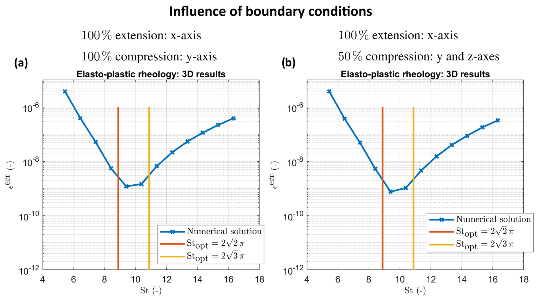
Figure 11 Numerical results in 3D (panels b and c): convergence in an elasto-plastic medium as a function of St. The parameter ϵ^err corresponds to the error magnitude of the APT scheme. Simulations in panels (a) and (b) are identical except for the different partitioning of pure shear boundary conditions.

6.4 Influence of initial conditions in 3D: elastic model

We consider a 3D numerical domain with $L_x=L_y=L_z=\mathrm{1}$. Figure 12 presents 3D numerical results for the elastic medium. Different panels correspond to identical simulations but with different initial conditions. The numerical outcomes are analyzed as a function of St. The total number of iterations over the pseudo-time is 1000, with a grid resolution of N=127³ cells. The results indicate that the optimal value of St is slightly different from $\mathit{St}=\mathrm{2}\mathit{\pi }\sqrt{\mathrm{3}}$. We attribute it to different initial conditions applied which are the combinations of cos and sin functions across x, y, and z axes.

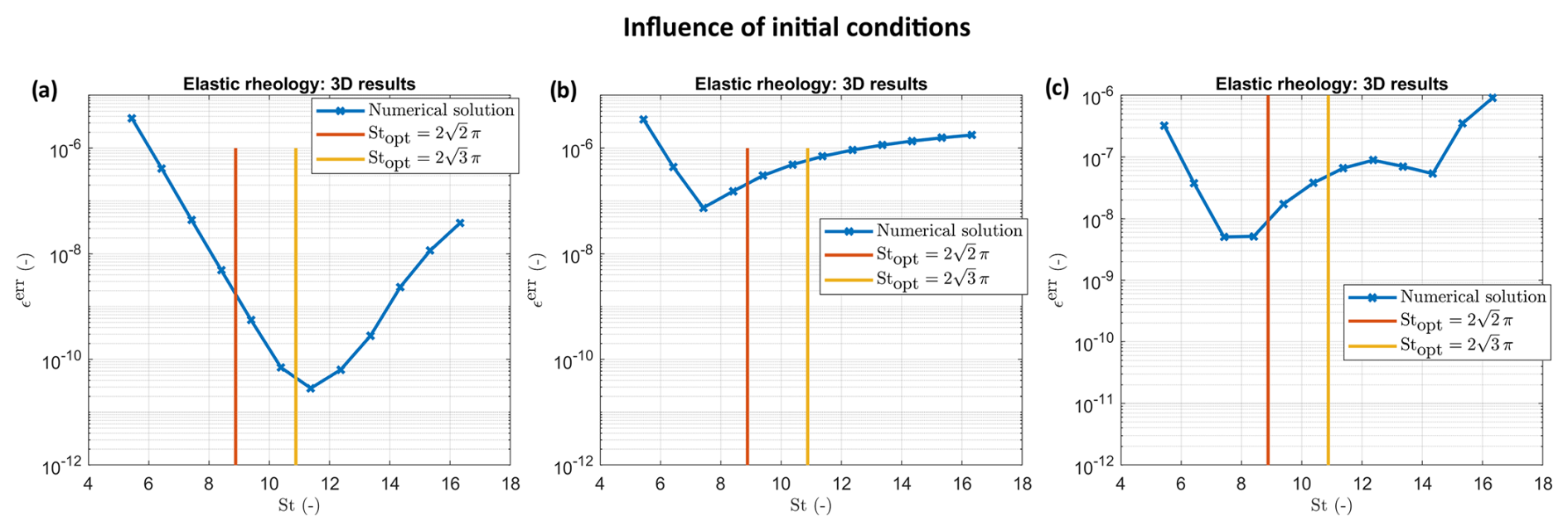
Figure 12 Numerical results in 3D (panels a, b, and c): convergence in an elastic medium as a function of St. The parameter ϵ^err corresponds to the error magnitude of the APT scheme. Simulations in panels (a), (b), and (c) are identical except for the different initial conditions. Panel (a) corresponds to initial conditions of cos function on the x, y, and z axes. Panel (b) corresponds to initial conditions of cos function on the x and y axes and sin function on the z axis. Panel (c) corresponds to initial conditions of sin function on the x, y, and z axes.

6.5 General applicability: influence of initial and boundary conditions, nonlinearities, and coupling

This study demonstrates that in homogeneous media with specific initial and boundary conditions, the optimal values of key numerical parameters, such as St_opt, can be accurately predicted across 1D, 2D, and 3D domains. This accuracy holds particularly true in the context of coupled systems of equations, as exemplified by the poroelastic models presented here. However, when dealing with more complex and realistic scenarios, special considerations are required to maintain this accuracy.

Our numerical experiments highlight that factors such as initial conditions, medium heterogeneities, and the presence of coupling and nonlinearities (e.g., plasticity) can influence the optimal values of numerical parameters. For instance, while in homogeneous and idealized conditions, the choice of St_opt may remain relatively stable, introducing a different initial condition necessitates a slight reassessment of these parameters. The study of strain localization (i.e., elasto-plastic rheology) in 3D models has shown that the presence of plasticity, which introduces strong nonlinearities, can slightly modify the convergence characteristics. The sensitivity of St_opt to boundary conditions was only minor in the 3D simulations. This suggests that our approach can provide a strong starting point for selecting numerical parameters. In practical applications, where media may be heterogeneous and boundary and initial conditions complex, this study provides a framework for estimating St_opt. However, to ensure the accuracy and efficiency of simulations, it is recommended to conduct additional test simulations. These tests are necessary to fine-tune the parameters based on the specific characteristics of the model.

7 Conclusions

In this study, we performed a comprehensive analysis of the accelerated pseudo-transient (APT) method for solving elastic, viscoelastic, and coupled hydromechanical problems, specifically those governed by quasi-static Biot poroelastic equations in 1D, 2D, and 3D domains. We identified the optimal numerical parameters for rapid convergence in elastic, viscoelastic, and poroelastic simulations, offering insights into the efficiency of the APT method across various spatial dimensions.

Our results demonstrated the method's effectiveness in handling complex coupled systems and its robustness in both homogeneous and heterogeneous media. By comparing numerical results with analytical solutions for elastic equations, we validated the accuracy and reliability of the APT method.

We explored the impact of initial and boundary conditions, nonlinearities, and coupling on optimal numerical parameters, emphasizing the importance of adaptability in real-world applications. While the APT method provides a strong framework for selecting numerical parameters, further refinement is often needed for practical applications.

To illustrate the APT method's flexibility, we addressed strain localization in 2D and 3D contexts using a poro-elasto-viscoplastic model, employing high resolutions (10 000² in 2D and 512³ in 3D), which has not been extensively explored before. This model, based on a hypoelastic constitutive framework, accommodates large strain simulations. All results are reproducible, and we have made the MATLAB code, Maple scripts, and CUDA C codes publicly available in a permanent repository.

Appendix A: First PT and APT methods

A1 The Richardson method for elliptic equations

Let us write the simplest version of the relaxation method to solve an elliptic equation of quasi-static elasticity:

$$\begin{array}{}\text{(A1)}& \left\{\begin{array}{l}{\mathit{\sigma }}_{xx}=(K+\frac{\mathrm{4}}{\mathrm{3}}G)\frac{\partial u_x}{\partial x}\\ \mathrm{0}=\frac{\partial {\mathit{\sigma }}_{xx}}{\partial x}-\mathit{\mu }\frac{\partial u_x}{\partial \stackrel{\mathrm{̃}}{t}},\end{array}\right.\end{array}$$

where u_x is the displacement, $\stackrel{\mathrm{̃}}{t}$ is a pseudo-time, and μ is a damping parameter. The system in Eq. (A1) represents a diffusive-type physical behavior in pseudo-time. The system is solved once the term $\partial u_x/\partial \stackrel{\mathrm{̃}}{t}$ converges to zero with a certain precision (e.g., 10⁻¹²). The convergence of this type of equation is $\sim n_x^{\mathrm{2}}$, where n_x is the number of grid cells in the x direction. Such a convergence rate makes this method impractical for large 3D problems; therefore, this method is not analyzed here. An interested reader can find more details in Frankel (1950).

A2 The accelerated pseudo-transient method: initial damping scheme

Now, let us consider a more advanced version of the pseudo-transient which we will call the accelerated pseudo-transient method (APT):

$$\begin{array}{}\text{(A2)}& \left\{\begin{array}{l}{\mathit{\sigma }}_{xx}=(K+\frac{\mathrm{4}}{\mathrm{3}}G)\frac{\partial u_x}{\partial x}\\ \stackrel{\mathrm{̃}}{\mathit{\rho }}\frac{\partial v_x}{\partial \stackrel{\mathrm{̃}}{t}}=\frac{\partial {\mathit{\sigma }}_{xx}}{\partial x}-\mathit{\mu }{v}_x\\ \frac{\partial u_x}{\partial t}=v_x,\end{array}\right.\end{array}$$

where μ and $\stackrel{\mathrm{̃}}{\mathit{\rho }}$ are the damping parameters, and t is the physical time which is linked to a loading increment. The system (Eq. A2) is solved once the terms $\partial v_x/\partial \stackrel{\mathrm{̃}}{t}$ and μv_x converge to zero with a certain precision (e.g., 10⁻¹²). The advantage of this system in Eq. (A2) over Eq. (A1) is that now the system in Eq. (A2) describes propagating waves in pseudo-physical space and pseudo-time (i.e., hyperbolic), and therefore the convergence rate is ∼n_x (compared to $\sim n_x^{\mathrm{2}}$ in the Richardson method for the elliptic equation, Eq. A1). An interested reader is referred to Poliakov et al. (1993b, a) for more details regarding this damping scheme.

Appendix B: Quasi-static elasticity equations

Let us decompose the stress tenor into the pressure and deviatoric stress tensor:

$$\begin{array}{}\text{(B1)}& {\mathit{\sigma }}_{xx}=-p+{\mathit{\tau }}_{xx}.\end{array}$$

Now, the system in Eq. (4) can be rewritten as

$$\begin{array}{}\text{(B2)}& \left\{\begin{array}{l}\frac{\partial p}{\partial t}=-K\frac{\partial v_x}{\partial x}\\ \frac{\partial {\mathit{\tau }}_{xx}}{\partial t}=\mathrm{2}G\left(\frac{\partial v_x}{\partial x}-\frac{\mathrm{1}}{\mathrm{3}}\frac{\partial v_x}{\partial x}\right)\\ \mathrm{0}=\frac{\partial (-p+{\mathit{\tau }}_{xx})}{\partial x}.\end{array}\right.\end{array}$$

The quasi-static elasticity in Eq. (B2) can then be rewritten with the pseudo-time $\stackrel{\mathrm{̃}}{t}$,

$$\begin{array}{}\text{(B3)}& \left\{\begin{array}{l}\frac{\mathrm{1}}{\stackrel{\mathrm{̃}}{K}}\frac{\partial p}{\partial \stackrel{\mathrm{̃}}{t}}+\frac{\mathrm{1}}{K}\frac{p-\widehat{p}}{\mathrm{\Delta }t}=-\frac{\partial v_x}{\partial x}\\ \frac{\mathrm{1}}{\mathrm{2}\stackrel{\mathrm{̃}}{G}}\frac{\partial {\mathit{\tau }}_{xx}}{\partial \stackrel{\mathrm{̃}}{t}}+\frac{\mathrm{1}}{\mathrm{2}G}\frac{{\mathit{\tau }}_{xx}-{\widehat{\mathit{\tau }}}_{xx}}{\mathrm{\Delta }t}=\left(\frac{\partial v_x}{\partial x}-\frac{\mathrm{1}}{\mathrm{3}}\frac{\partial v_x}{\partial x}\right)\\ \stackrel{\mathrm{̃}}{\mathit{\rho }}\frac{\partial v_x}{\partial \stackrel{\mathrm{̃}}{t}}=-\frac{\partial {\mathit{\sigma }}_{xx}}{\partial x},\end{array}\right.\end{array}$$

where $\widehat{p}$ is the pressure field at the previous physical time step and ${\widehat{\mathit{\tau }}}_{xx}$ in the deviatoric stress at the previous physical time step.

The system in Eq. (B3) can be simplified:

$$\begin{array}{}\text{(B4)}& \left\{\begin{array}{l}\frac{\mathrm{1}}{\stackrel{\mathrm{̃}}{K}}\frac{\partial p}{\partial \stackrel{\mathrm{̃}}{t}}+\frac{\mathrm{1}}{K}\frac{p}{\mathrm{\Delta }t}=-\frac{\partial v_x}{\partial x}\\ \frac{\mathrm{1}}{\mathrm{2}\stackrel{\mathrm{̃}}{G}}\frac{\partial {\mathit{\tau }}_{xx}}{\partial \stackrel{\mathrm{̃}}{t}}+\frac{\mathrm{1}}{\mathrm{2}G}\frac{{\mathit{\tau }}_{xx}}{\mathrm{\Delta }t}=\left(\frac{\partial v_x}{\partial x}-\frac{\mathrm{1}}{\mathrm{3}}\frac{\partial v_x}{\partial x}\right)\\ \stackrel{\mathrm{̃}}{\mathit{\rho }}\frac{\partial v_x}{\partial \stackrel{\mathrm{̃}}{t}}=-\frac{\partial (-p+{\mathit{\tau }}_{xx})}{\partial x}.\end{array}\right.\end{array}$$

$\stackrel{\mathrm{̃}}{H}=\stackrel{\mathrm{̃}}{K}+\frac{\mathrm{4}}{\mathrm{3}}\stackrel{\mathrm{̃}}{G}=K+\frac{\mathrm{4}}{\mathrm{3}}G$, $\stackrel{\mathrm{̃}}{K}=K$, and $\stackrel{\mathrm{̃}}{G}=G$. The optimal value of St is the same as for the system in Eq. (5) (or Eq. 6):

$$\begin{array}{}\text{(B5)}& \mathit{St}={\mathit{St}}_{\text{opt}}=\mathrm{2}\mathit{\pi },\end{array}$$

which corresponds to the fastest attenuation of propagating waves. The stress tenor in decomposed into the pressure and deviatoric stress tensor; therefore, the following expressions are also provided:

$$\begin{array}{}\text{(B6)}& \stackrel{\mathrm{̃}}{G}\mathrm{\Delta }\stackrel{\mathrm{̃}}{t}=({\stackrel{\mathrm{̃}}{V}}_{\mathrm{p}}\mathrm{\Delta }\stackrel{\mathrm{̃}}{t}{)}^{\mathrm{2}}{\left({\displaystyle \frac{\mathrm{\Delta }\stackrel{\mathrm{̃}}{t}}{\stackrel{\mathrm{̃}}{\mathit{\rho }}}}\right)}^{-\mathrm{1}}{\left(K_G+{\displaystyle \frac{\mathrm{4}}{\mathrm{3}}}\right)}^{-\mathrm{1}},\end{array}$$

where $K_G=K/G$, and

$$\begin{array}{}\text{(B7)}& \stackrel{\mathrm{̃}}{K}\mathrm{\Delta }\stackrel{\mathrm{̃}}{t}=K_G\stackrel{\mathrm{̃}}{G}\mathrm{\Delta }\stackrel{\mathrm{̃}}{t}.\end{array}$$

Appendix C: Discretization: quasi-static elasticity equations

Let us write the discrete form of the system (Eq. 6). We use a classical conservative staggered space–time grid discretization (Virieux, 1986) which is equivalent to a finite-volume approach (Dormy and Tarantola, 1995). More details on the present discretization can be found in Alkhimenkov et al. (2021b, a). Let us consider a physical domain L_x that is discretized into grid cells such that L_x=n_x Δx. The physical time t is also discretized as Δt ($\mathrm{\Delta }\stackrel{\mathrm{̃}}{t}$ is the pseudo-time). The resulting discrete form of the system (Eq. 6) is

$$\begin{array}{}\text{(C1)}& \left\{\begin{array}{l}\frac{\mathrm{1}}{\stackrel{\mathrm{̃}}{H}}\frac{[{\mathit{\sigma }}_{xx}{]}_i^{l+\mathrm{1}/\mathrm{2}}-[{\mathit{\sigma }}_{xx}{]}_i^{l-\mathrm{1}/\mathrm{2}}}{\mathrm{\Delta }\stackrel{\mathrm{̃}}{t}}+\frac{\mathrm{1}}{H}\frac{[{\mathit{\sigma }}_{xx}{]}_i^{l+\mathrm{1}/\mathrm{2}}}{\mathrm{\Delta }t}=\frac{[v_x{]}_{i+\mathrm{1}/\mathrm{2}}^l-[v_x{]}_{i-\mathrm{1}/\mathrm{2}}^l}{\mathrm{\Delta }x}\\ \stackrel{\mathrm{̃}}{\mathit{\rho }}\frac{[v_x{]}_{i+\mathrm{1}/\mathrm{2}}^{l+\mathrm{1}}-[v_x{]}_{i+\mathrm{1}/\mathrm{2}}^l}{\mathrm{\Delta }\stackrel{\mathrm{̃}}{t}}=\frac{[{\mathit{\sigma }}_{xx}{]}_{i+\mathrm{1}}^{l+\mathrm{1}/\mathrm{2}}-[{\mathit{\sigma }}_{xx}{]}_i^{l+\mathrm{1}/\mathrm{2}}}{\mathrm{\Delta }x}.\end{array}\right.\end{array}$$

The discrete form of the system (Eq. B3) can be written as

$$\begin{array}{}\text{(C2)}& \left\{\begin{array}{l}\frac{\mathrm{1}}{\stackrel{\mathrm{̃}}{K}}\frac{p_i^{l+\mathrm{1}/\mathrm{2}}-p_i^{l-\mathrm{1}/\mathrm{2}}}{\mathrm{\Delta }\stackrel{\mathrm{̃}}{t}}+\frac{\mathrm{1}}{K}\frac{p_i^{l+\mathrm{1}/\mathrm{2}}-{\widehat{p}}_i^{l+\mathrm{1}/\mathrm{2}}}{\mathrm{\Delta }t}=-\frac{[v_x{]}_{i+\mathrm{1}/\mathrm{2}}^l-[v_x{]}_{i-\mathrm{1}/\mathrm{2}}^l}{\mathrm{\Delta }x}\\ \frac{\mathrm{1}}{\mathrm{2}\stackrel{\mathrm{̃}}{G}}\frac{[{\mathit{\tau }}_{xx}{]}_i^{l+\mathrm{1}/\mathrm{2}}-[{\mathit{\tau }}_{xx}{]}_i^{l-\mathrm{1}/\mathrm{2}}}{\mathrm{\Delta }\stackrel{\mathrm{̃}}{t}}+\frac{\mathrm{1}}{\mathrm{2}G}\frac{[{\mathit{\tau }}_{xx}{]}_i^{l+\mathrm{1}/\mathrm{2}}-[{\widehat{\mathit{\tau }}}_{xx}{]}_i^{l+\mathrm{1}/\mathrm{2}}}{\mathrm{\Delta }t}=\mathrm{\dots }\\ =\left(\frac{[v_x{]}_{i+\mathrm{1}/\mathrm{2}}^l-[v_x{]}_{i-\mathrm{1}/\mathrm{2}}^l}{\mathrm{\Delta }x}-\frac{\mathrm{1}}{\mathrm{3}}\frac{[v_x{]}_{i+\mathrm{1}/\mathrm{2}}^l-[v_x{]}_{i-\mathrm{1}/\mathrm{2}}^l}{\mathrm{\Delta }x}\right)\\ \stackrel{\mathrm{̃}}{\mathit{\rho }}\frac{[v_x{]}_{i+\mathrm{1}/\mathrm{2}}^{l+\mathrm{1}}-[v_x{]}_{i+\mathrm{1}/\mathrm{2}}^l}{\mathrm{\Delta }\stackrel{\mathrm{̃}}{t}}=-\frac{(-(p_{i+\mathrm{1}}^{l+\mathrm{1}/\mathrm{2}}-p_i^{l+\mathrm{1}/\mathrm{2}})+[{\mathit{\tau }}_{xx}{]}_{i+\mathrm{1}}^{l+\mathrm{1}/\mathrm{2}}-\left[{\mathit{\tau }}_{xx}{]}_i^{l+\mathrm{1}/\mathrm{2}}\right)}{\mathrm{\Delta }x}.\end{array}\right.\end{array}$$

Appendix D: MATLAB code

Listing D1 MATLAB code for time loop computations.

Appendix E: Discretization: viscoelasticity

The discrete form of the system (Eq. 26) can be written as

$$\begin{array}{}\text{(E1)}& \left\{\begin{array}{l}\frac{\mathrm{1}}{\stackrel{\mathrm{̃}}{K}}\frac{p_i^{l+\mathrm{1}/\mathrm{2}}-p_i^{l-\mathrm{1}/\mathrm{2}}}{\mathrm{\Delta }\stackrel{\mathrm{̃}}{t}}+\frac{\mathrm{1}}{K}\frac{p_i^{l+\mathrm{1}/\mathrm{2}}}{\mathrm{\Delta }t}=-\frac{[v_x{]}_{i+\mathrm{1}/\mathrm{2}}^l-[v_x{]}_{i-\mathrm{1}/\mathrm{2}}^l}{\mathrm{\Delta }x}\\ \frac{\mathrm{1}}{\mathrm{2}\stackrel{\mathrm{̃}}{G}}\frac{[{\mathit{\tau }}_{xx}{]}_i^{l+\mathrm{1}/\mathrm{2}}-[{\mathit{\tau }}_{xx}{]}_i^{l-\mathrm{1}/\mathrm{2}}}{\mathrm{\Delta }\stackrel{\mathrm{̃}}{t}}+\frac{\mathrm{1}}{\mathrm{2}G}\frac{[{\mathit{\tau }}_{xx}{]}_i^{l+\mathrm{1}/\mathrm{2}}-[{\widehat{\mathit{\tau }}}_{xx}{]}_i^{l+\mathrm{1}/\mathrm{2}}}{\mathrm{\Delta }t}+\frac{[{\mathit{\tau }}_{xx}{]}_i^{l+\mathrm{1}/\mathrm{2}}}{\mathrm{2}{\mathit{\mu }}_{\mathrm{s}}}=\mathrm{\dots }\\ =\left(\frac{[v_x{]}_{i+\mathrm{1}/\mathrm{2}}^l-[v_x{]}_{i-\mathrm{1}/\mathrm{2}}^l}{\mathrm{\Delta }x}-\frac{\mathrm{1}}{\mathrm{3}}\frac{[v_x{]}_{i+\mathrm{1}/\mathrm{2}}^l-[v_x{]}_{i-\mathrm{1}/\mathrm{2}}^l}{\mathrm{\Delta }x}\right)\\ \stackrel{\mathrm{̃}}{\mathit{\rho }}\frac{[v_x{]}_{i+\mathrm{1}/\mathrm{2}}^{l+\mathrm{1}}-[v_x{]}_{i+\mathrm{1}/\mathrm{2}}^l}{\mathrm{\Delta }\stackrel{\mathrm{̃}}{t}}=-\frac{(-(p_{i+\mathrm{1}}^{l+\mathrm{1}/\mathrm{2}}-p_i^{l+\mathrm{1}/\mathrm{2}})+[{\mathit{\tau }}_{xx}{]}_{i+\mathrm{1}}^{l+\mathrm{1}/\mathrm{2}}-\left[{\mathit{\tau }}_{xx}{]}_i^{l+\mathrm{1}/\mathrm{2}}\right)}{\mathrm{\Delta }x}.\end{array}\right.\end{array}$$

Appendix F: Discretization: quasi-static Biot poroelastic equations

The discrete form of the system in Eqs. (41)–(43) can be written as

$$\begin{array}{}\text{(F1)}& {\displaystyle }\left\{\begin{array}{l}\frac{\mathrm{1}}{{\stackrel{\mathrm{̃}}{K}}_{\mathrm{1}}}\frac{[\stackrel{\mathrm{‾}}{p}{]}_i^{l+\mathrm{1}/\mathrm{2}}-[\stackrel{\mathrm{‾}}{p}{]}_i^{l-\mathrm{1}/\mathrm{2}}}{\mathrm{\Delta }\stackrel{\mathrm{̃}}{t}}+\frac{\mathrm{1}}{K_{\mathrm{u}}}\frac{[\stackrel{\mathrm{‾}}{p}{]}_i^{l+\mathrm{1}/\mathrm{2}}-[\widehat{\stackrel{\mathrm{‾}}{p}}{]}_i^{l+\mathrm{1}/\mathrm{2}}}{\mathrm{\Delta }t}\\ =-\frac{[v_x{]}_{i+\mathrm{1}/\mathrm{2}}^l-[v_x{]}_{i-\mathrm{1}/\mathrm{2}}^l}{\mathrm{\Delta }x}-B\frac{[q_x^{\mathrm{D}}{]}_{i+\mathrm{1}/\mathrm{2}}^l-[q_x^{\mathrm{D}}{]}_{i-\mathrm{1}/\mathrm{2}}^l}{\mathrm{\Delta }x}\\ \frac{\mathrm{1}}{{\stackrel{\mathrm{̃}}{K}}_{\mathrm{2}}}\frac{[p_{\mathrm{f}}{]}_i^{l+\mathrm{1}/\mathrm{2}}-[p_{\mathrm{f}}{]}_i^{l-\mathrm{1}/\mathrm{2}}}{\mathrm{\Delta }\stackrel{\mathrm{̃}}{t}}+\frac{\mathrm{1}}{K_{\mathrm{u}}}\frac{[p_{\mathrm{f}}{]}_i^{l+\mathrm{1}/\mathrm{2}}-[{\widehat{p}}_{\mathrm{f}}{]}_i^{l+\mathrm{1}/\mathrm{2}}}{\mathrm{\Delta }t}\\ =-B\frac{[v_x{]}_{i+\mathrm{1}/\mathrm{2}}^l-[v_x{]}_{i-\mathrm{1}/\mathrm{2}}^l}{\mathrm{\Delta }x}-\frac{B}{\mathit{\alpha }}\frac{[q_x^{\mathrm{D}}{]}_{i+\mathrm{1}/\mathrm{2}}^l-[q_x^{\mathrm{D}}{]}_{i-\mathrm{1}/\mathrm{2}}^l}{\mathrm{\Delta }x}\end{array},\right.\text{(F2)}& {\displaystyle }\left\{\begin{array}{l}\frac{\mathrm{1}}{\mathrm{2}\stackrel{\mathrm{̃}}{G}}\frac{[{\stackrel{\mathrm{‾}}{\mathit{\tau }}}_{xx}{]}_i^{l+\mathrm{1}/\mathrm{2}}-[{\stackrel{\mathrm{‾}}{\mathit{\tau }}}_{xx}{]}_i^{l-\mathrm{1}/\mathrm{2}}}{\mathrm{\Delta }\stackrel{\mathrm{̃}}{t}}+\frac{\mathrm{1}}{\mathrm{2}{G}_{\mathrm{u}}}\frac{[{\stackrel{\mathrm{‾}}{\mathit{\tau }}}_{xx}{]}_i^{l+\mathrm{1}/\mathrm{2}}}{\mathrm{\Delta }t}\\ =\left(\frac{[v_x{]}_{i+\mathrm{1}/\mathrm{2}}^l-[v_x{]}_{i-\mathrm{1}/\mathrm{2}}^l}{\mathrm{\Delta }x}-\frac{\mathrm{1}}{\mathrm{3}}\frac{[v_x{]}_{i+\mathrm{1}/\mathrm{2}}^l-[v_x{]}_{i-\mathrm{1}/\mathrm{2}}^l}{\mathrm{\Delta }x}\right)\end{array},\right.\text{(F3)}& {\displaystyle }\left\{\begin{array}{l}{\stackrel{\mathrm{̃}}{\mathit{\rho }}}_{\mathrm{t}}\frac{[v_x{]}_{i+\mathrm{1}/\mathrm{2}}^{l+\mathrm{1}}-[v_x{]}_{i+\mathrm{1}/\mathrm{2}}^l}{\mathrm{\Delta }\stackrel{\mathrm{̃}}{t}}\\ =-\frac{(-([\stackrel{\mathrm{‾}}{p}{]}_{i+\mathrm{1}}^{l+\mathrm{1}/\mathrm{2}}-[\stackrel{\mathrm{‾}}{p}{]}_i^{l+\mathrm{1}/\mathrm{2}})+[{\stackrel{\mathrm{‾}}{\mathit{\tau }}}_{xx}{]}_{i+\mathrm{1}}^{l+\mathrm{1}/\mathrm{2}}-\left[{\stackrel{\mathrm{‾}}{\mathit{\tau }}}_{xx}{]}_i^{l+\mathrm{1}/\mathrm{2}}\right)}{\mathrm{\Delta }x}\\ {\stackrel{\mathrm{̃}}{\mathit{\rho }}}_{\mathrm{a}}\frac{[q_x^{\mathrm{D}}{]}_{i+\mathrm{1}/\mathrm{2}}^{l+\mathrm{1}}-[q_x^{\mathrm{D}}{]}_{i+\mathrm{1}/\mathrm{2}}^l}{\mathrm{\Delta }\stackrel{\mathrm{̃}}{t}}=-[q_x^{\mathrm{D}}{]}_{i+\mathrm{1}/\mathrm{2}}^l\\ -\frac{\frac{k}{{\mathit{\eta }}_{\mathrm{f}}}\left(\right[p_{\mathrm{f}}{]}_{i+\mathrm{1}}^{l+\mathrm{1}/\mathrm{2}}-\left[p_{\mathrm{f}}{]}_i^{l+\mathrm{1}/\mathrm{2}}\right)}{\mathrm{\Delta }x}\end{array}.\right.\end{array}$$