A flexible Regional Ocean Modeling System-based hybrid coupled model for El Niño–Southern Oscillation studies – model formulation and performance evaluation

El Niño–Southern Oscillation (ENSO) constitutes the most prominent interannual climate variation mode in the climate system that originates from ocean–atmosphere interactions in the tropical Pacific. Accurately modeling ENSO variation has consistently posed a great challenge, exhibiting strongly model-dependent representations and simulations of ENSO. This study presents a novel hybrid coupled model (HCM), denoted HCM_ROMS, built upon the Regional Ocean Modeling System (ROMS) that has been widely used for regional modeling studies. For basin-wide applications to the tropical Pacific, here, the ROMS is coupled with a statistical atmospheric model. The statistical atmospheric model is based on singular value decomposition (SVD), capturing interannual relationships of atmospheric perturbations such as wind stress and freshwater flux anomalies with sea surface temperature (SST) anomalies. The model is constructed in a flexible way so that various components representing atmospheric forcing and oceanic biogeochemistry can be easily included as a module in the HCM_ROMS. Results demonstrate that the HCM_ROMS can simulate a stable quasi-3-year ENSO cycle when the interannual wind stress coupling coefficient, α_τ, is set to 1.5. The HCM_ROMS reproduces the three-dimensional (3D) evolution of ENSO-related anomalies, revealing that the most pronounced temperature anomalies occur beneath the surface at 150 m. The interannual temperature anomaly budget highlights the dominance of the advection process in simulated ENSO. Vertical mixing contributes negatively to ENSO anomalies, damping temperature anomalies from the surface due to the turbulent heat flux feedback. This newly developed HCM_ROMS is poised to serve as an efficient modeling tool for ENSO research in the future.

1 Introduction

El Niño–Southern Oscillation (ENSO), characterized by a warm-phase (El Niño) and a cold-phase (La Niña) sea surface temperature, occurs approximately every 2–7 years, representing the most prominent interannual climate variation mode on the Earth. ENSO greatly influences human and natural systems, reshaping global atmospheric circulation and weather systems (Yeh et al., 2018). It leads to extreme weather and climate events such as floods, droughts, and heat waves (McPhaden et al., 2006). Thus, the accurate prediction of ENSO holds vital importance across various application sectors, including agricultural production, food security, freshwater resources, and the economy worldwide.

ENSO originates in the tropical Pacific through coupled ocean and atmosphere interactive processes (Bjerknes, 1969; Zebiak and Cane, 1987). The onset of ENSO is triggered by the reinforcing Bjerknes feedback among wind, sea surface temperature (SST), and the thermocline. During El Niño, an initial positive SST anomaly (SSTA) in the eastern Pacific reduces the east–west SST gradient, weakening the Walker circulation and thus the reduction in the easterly trade winds (Lindzen and Nigam, 1987). The weaker trade winds have two impacts on the ocean. On one hand, they reduce the equatorial upwelling in the eastern Pacific, causing the warm SST anomaly over the eastern basin. On the other hand, the weaker trade winds facilitate the eastward migration of surface warm water from the western Pacific warm pool. The eastward migration of surface warm water raises SST east of the dateline, triggering the eastward shift in deep convection. This, in turn, further relaxes the trade winds to the west of the convective center, causing positive feedback that influences the SST rise. During the cold phase of ENSO, La Niña's onset is the same as El Niño but with the opposite sign (Latif et al., 1994).

The phase transition of ENSO (i.e., the transition between El Niño and La Niña) is more complex. The ENSO cycle can be affected by the wind-driven Kelvin waves and the reflected Kelvin and Rossby waves at the western and eastern boundaries of the Pacific, respectively; by discharge–recharge processes due to Sverdrup transport; and by anomalous zonal advection. These processes are named, in turn, in previous studies: the western Pacific oscillator (Wang et al., 1999; Weisberg and Wang, 1997), the delayed oscillator (Battisti and Hirst, 1989; Suarez and Schopf, 1988), the recharge oscillator (Jin, 1997a, b), and the advective–reflective oscillator (Picaut et al., 1997). All these oscillators can work together as a unified oscillator to affect the ENSO cycle (Wang, 2001). Extratropical processes also affect ENSO, as the thermal and salinity anomalies in the northern Pacific can be conveyed to the tropical Pacific along the subtropical cell (Gu and Philander, 1997; Kleeman et al., 1999; McCreary and Lu, 1994; Zhang et al., 1998; Zhou and Zhang, 2022a). In addition, ENSO can be affected by various forcing and feedback processes such as stochastic atmospheric forcing (Jin et al., 2007; Moore and Kleeman, 1999; Zhang et al., 2008), freshwater flux (Gao et al., 2020; Kang et al., 2014; Zhang et al., 2012), ocean-biology-induced feedback (Shi et al., 2023; Tian et al., 2020; Zhang et al., 2018b), and tropical instability waves (Tian et al., 2019; Zhang, 2016; Zhang et al., 2023). Given the intricate interplay among these effects, comprehending the individual and collective impacts of these processes on ENSO poses a great challenge.

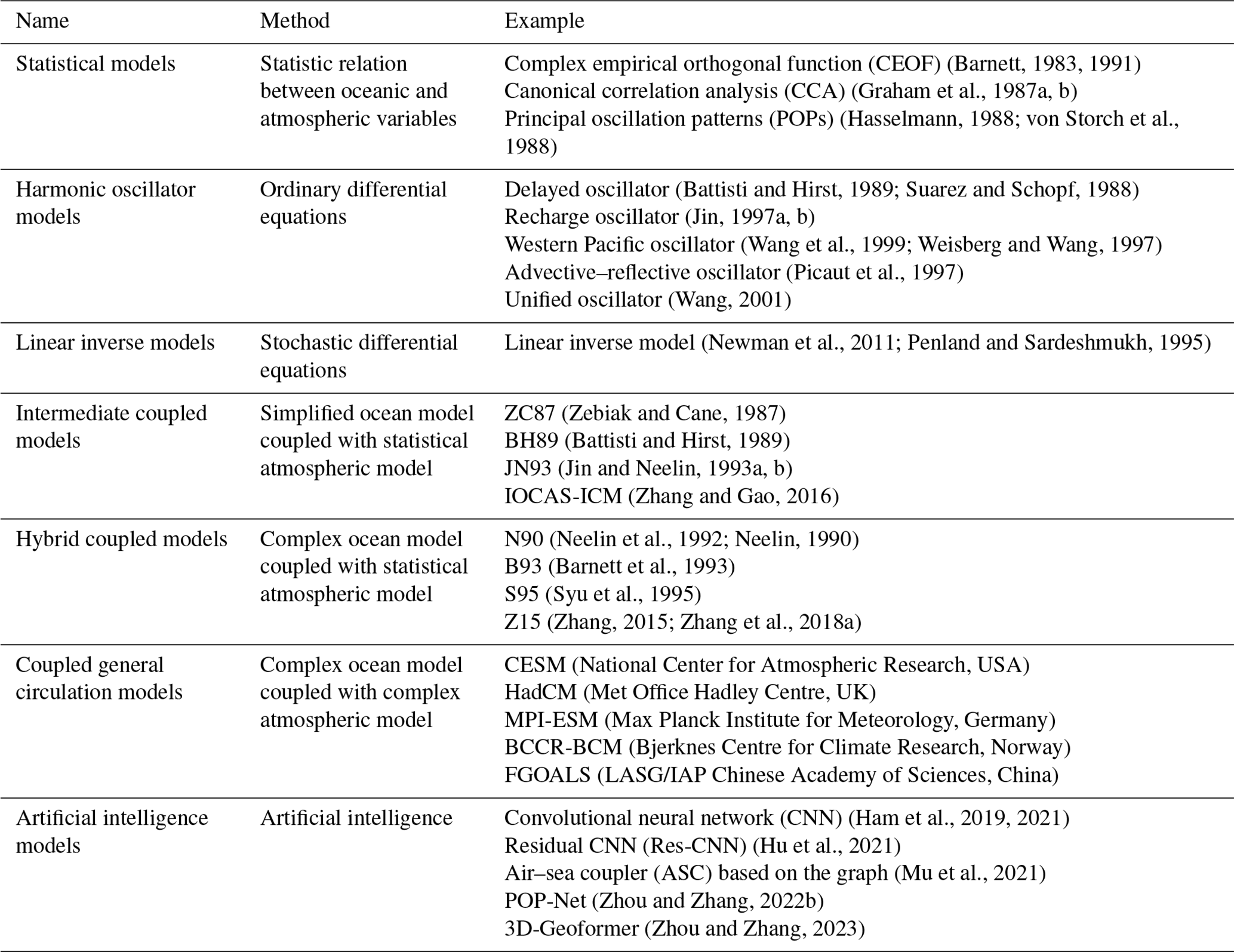
Numerical models are powerful tools for investigating and predicting ENSO. Over the past decades, a variety of coupled models, encompassing different levels of complexity in both the ocean and atmosphere components, have been developed for ENSO studies. These models can be categorized according to their approaches, such as the statistical model (SM), harmonic oscillator model (HOM), linear inverse model (LIM), intermediate coupled model (ICM), hybrid coupled model (HCM), coupled general circulation model (CGCM), and artificial intelligence (AI); their characteristics are listed in Table 1. Each of these models boasts unique advantages in the realm of ENSO study. In particular, the HCM, which combines a comprehensive ocean general circulation model (OGCM) with a simplified atmospheric model, excels at incorporating complete ocean dynamic and thermodynamic processes without exhibiting notable climate drift issues (Zhang et al., 2020). The advantage of HCM is the representation of atmospheric forcing in anomaly form, where interannual perturbations are considered in the model. This can isolate the interannual forcing and feedback effects in a clear way, better enhancing the understanding of ENSO mechanisms (McCreary and Anderson, 1991; Zhang et al., 2020).

Table 1 List of the coupled models for ENSO investigation.

In a previous study, Zhang (2015) developed an HCM (Z15 hereafter) based on an OGCM and a statistical atmospheric model for interannual wind stress. The Z15 model successfully reproduces the quasi-4-year oscillation characteristics of ENSO (Gao et al., 2020; Zhang, 2015). However, despite various advantages of the Z15 model, such as simple model architecture and high computational efficiency, simulated El Niño (indicated by the positive SSTA) in the Z15 model is located near the dateline, suggesting a central Pacific instead of the typical eastern Pacific El Niño in the Z15 model (Gao et al., 2020; Zhang et al., 2018a). This is partly due to the use of the Gent–Cane OGCM (Gent and Cane, 1989) in the Z15 model, which is a reduced-gravity ocean model with a limited ability to simulate deep-temperature variations. The uppermost layer of the Gent–Cane OGCM is treated as a uniform mixed layer, with its depth determined by a bulk mixing parameterization (Chen et al., 1994). The bulk layer constraint hinders the Z15 model's ability to simulate vertical structure within the mixed layer. In addition, the Gent–Cane OGCM exhibits a restricted ability to simulate multiscale dynamic processes, such as ocean mesoscale eddies and tropical instability waves. All the aforementioned points underscore the urgent need to replace the Gent–Cane OGCM in the Z15 model with an advanced ocean model to better simulate and investigate ENSO mechanisms. Therefore, in this study, we attempt to develop a new HCM based on the state-of-the-art Regional Ocean Modeling System (ROMS). Such an HCM_ROMS can provide more detailed 3D ocean structure changes during ENSO evolution and help to explore ENSO mechanisms.

The objective of this study is to introduce the newly developed HCM_ROMS and assess its performance. The paper is structured as follows: Sect. 2 introduces the HCM_ROMS, including its statistical atmospheric model component, the ROMS setting, the HCM framework, and the numerical experimental design used in this study. Section 3 illustrates the performance of the HCM_ROMS. Summaries are provided in Sect. 4.

2 Numerical model and experimental design

2.1 Statistical atmospheric model

Following the Z15 modeling framework, a statistical atmospheric model is developed to represent the interannual perturbation fields of the atmosphere using singular value decomposition (SVD) analysis (Zhang, 2015). Figure 1 illustrates the schematic diagram of the statistical atmospheric model. The coupling relationship between any two interannual variation signals, such as SSTA and the wind stress anomaly (X and Y in Fig. 1a), can be established by decomposing their covariance matrix using SVD (Fig. 1a). In an SVD analysis, the left-singular vector (L in Fig. 1a) and right-singular vector (R in Fig. 1a) of the covariance matrix (S in Fig. 1a) serve as eigenvectors for the left field X and right field Y, respectively (Fig. 1a). Notably, the left-singular vector L and right-singular vector R share the same singular value Γ. Therefore, given a specific left field (Xm), the corresponding right-field signal (Ym) can be determined by SVD relation through the inversion process shown in Fig. 1b.

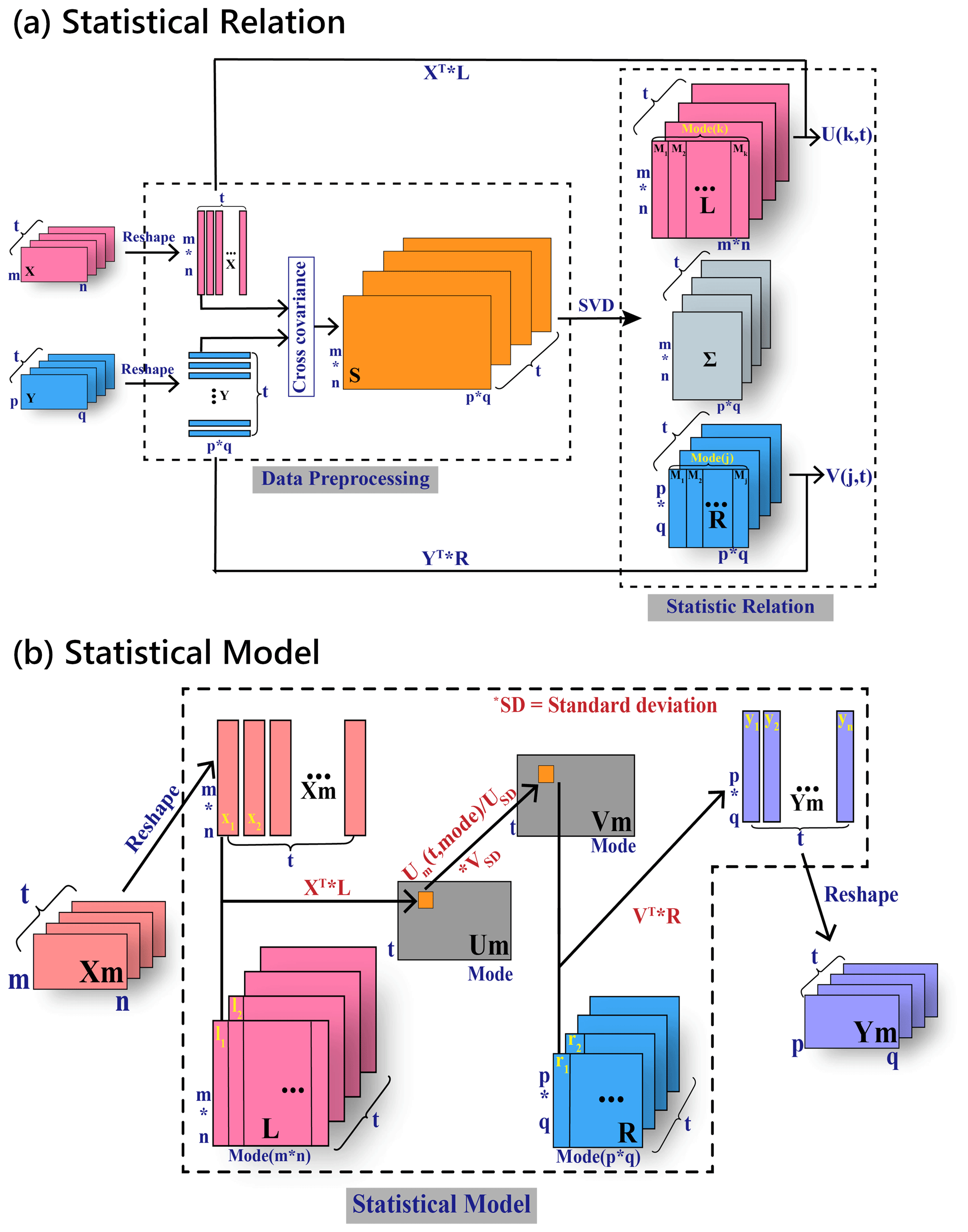
Figure 1 Flow chart of the (a) SVD analysis and (b) SVD-based statistical model. X and Y in (a) are the original interannual variation signals before SVD; S is the covariance matrix between X and Y; L is the left-singular vector and R is the right-singular vector; U and V are the time series of the left-singular vector and right-singular vector, respectively; and Γ is the singular value matrix. Xm in (b) is the left field input to the statistical model, Ym is the right field output, and Um and Vm are the calculated time series of left field and right field in the statistical model, respectively.

To include the ENSO-related atmospheric forcing–feedback processes in HCM_ROMS, we established statistical relations between the interannual SSTA (SST_inter) and both interannual wind stress anomalies (τ_inter) and interannual freshwater flux anomalies (FWF_inter) using the SVD analysis (Fig. 1a). It should be noted that the freshwater flux (FWF) in this work is defined as the net freshwater flux into the ocean, which is represented by the total precipitation (P) minus evaporation (E), i.e., P−E. The monthly SST_inter used to construct empirical statistical relations are derived from the National Oceanic and Atmospheric Administration (NOAA) Optimum Interpolation (OI) SST dataset with a spatial resolution of 1°×1° from 1981 to 1999 (Reynolds et al., 2002). The monthly τ_inter and FWF_inter come from a 24-member ensemble of the European Centre Hamburg Model (ECHAM) version 4.5 simulations forced by observed SST from 1950 to 1999 (Roeckner et al., 1996). Ensemble-averaged τ_inter and FWF_inter from the ECHAM simulations is used to reduce the impacts of atmospheric noise (Zhang et al., 2003).

The first SVD modes for SST_inter, τ_inter, and FWF_inter are shown in Fig. 2a–c, respectively. We note that since the first SVD mode of SST_inter in the SST_inter–τ_inter and SST_inter–FWF_inter pairings is similar, only the first SVD mode of SST_inter from the SST_inter–τ_inter pairing is shown in Fig. 2a. It shows that the SVD patterns include ENSO-related forcing and response processes. For example, the El Niño-type SSTA in the equatorial eastern Pacific (Fig. 2a) is associated with the tropical westerly wind stress anomalies (Fig. 2b) and FWF anomalies around the dateline (Fig. 2c). We calculated the squared covariance fractions of different SVD modes. The first five SVD modes can contribute 99.4 % of the τ_inter variations and 97.6 % of the FWF_inter variations. Therefore, we only include the first five SVD modes in the statistical atmospheric model to reproduce the interannual atmospheric forcing. The performance of the statistical atmospheric model at reproducing the τ_inter and FWF_inter is evaluated in Sect. 3.1.

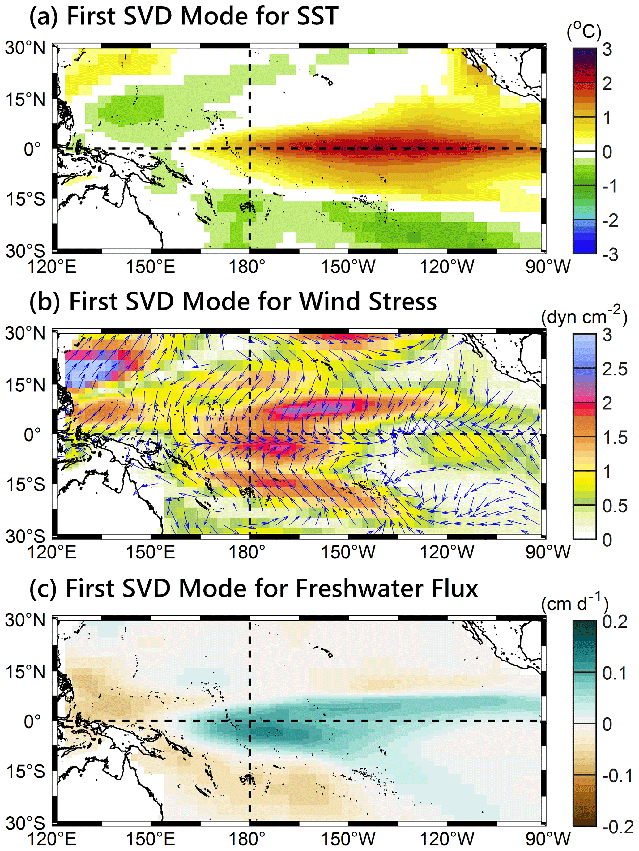
Figure 2 First SVD modes for the (a) interannual SSTA, (b) interannual wind stress anomaly, and (c) interannual freshwater flux anomaly.

2.2 The Regional Ocean Modeling System (ROMS) model

The comprehensive ocean model used in HCM_ROMS is based on the Regional Ocean Modeling System (ROMS) (Shchepetkin and Mcwilliams, 2005). ROMS is a community regional ocean model suitable for various applications in ocean forecasting and research. ROMS incorporates accurate and efficient physical and numerical algorithms. For example, all 2D and 3D equations in ROMS undergo time discretization using a third-order predictor and a corrector time-stepping algorithm (Shchepetkin and Mcwilliams, 2005). The enhanced stability of the scheme allows for larger time steps, which is important for climate simulations that need to be integrated for long periods. In addition, ROMS employs an explicit time-splitting scheme to solve the hydrostatic primitive equations for momentum. Within each baroclinic (3D, solving the primitive equations) time step, a finite number of barotropic (2D, solving the shallow-water equations) time steps are executed to evolve the free-surface and vertically integrated momentum equations. The time-splitting method allows the ROMS model to simulate and ensure the stability of high-frequency waves, increasing the model's accuracy in simulating the sea level variations.

Figure 3 shows the domain setting of the ROMS model used in this study. The ROMS model, with a horizontal resolution of 0.5°×0.5° (∼52.9 km × 52.9 km) covers the tropical Pacific ranging from 30° S to 30° N and from 95° E to 70° W. It should be noted that the limited domain of 30° S–30° N excludes extratropical dynamics, which also influences ENSO. The present study primarily focuses on air–sea coupling processes within the tropical Pacific. The role of extratropical influences will be addressed in future work, potentially through enhanced lateral boundary forcing or an expanded model domain. The ROMS model has 50 layers in the vertical direction, with a higher resolution (∼0.1 m on the model grid, with a water depth of 5000 m) near the sea surface using a terrain-following S coordinate with Shchepetkin's double-stretching function (Shchepetkin and Mcwilliams, 2009). The ROMS parametrizations include the nonlocal K-profile scheme for vertical mixing (Large et al., 1994) and the Smagorinsky scheme for horizontal diffusion (Smagorinsky, 1963). The shortwave radiation penetration into the ocean is calculated by a double-exponential irradiance absorption scheme (Paulson and Simpson, 1977), with Jerlov water type I parameters over the open ocean and Jerlov water type II parameters over the marginal seas (Kuo et al., 2023; Yu et al., 2017, 2020, 2022).

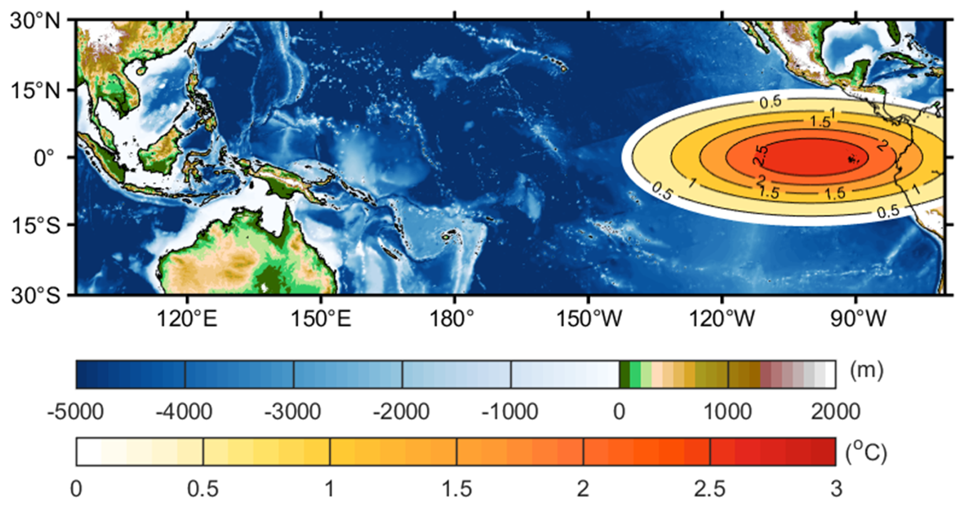
Figure 3 ROMS model domain and topography. The contours with orange shading show the El Niño-like SSTA, which drives the statistical atmospheric model during the initial kick for 8 months.

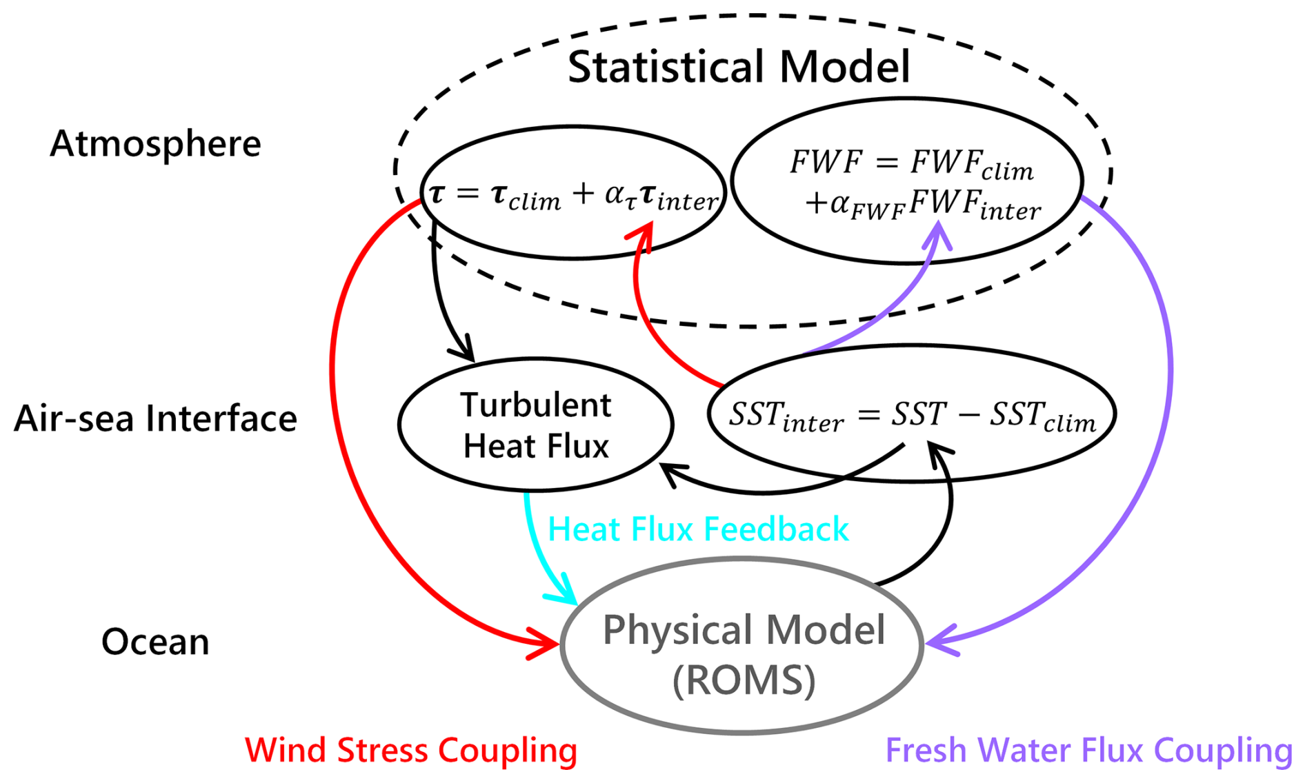
Figure 4 Schematic diagram of the HCM_ROMS. Red arrows represent wind stress coupling, purple arrows represent the FWF coupling, and the light-blue arrow represents the heat flux feedback.

2.3 Hybrid coupled model framework

Figure 4 illustrates the schematic diagram of the HCM_ROMS. It consists of the statistical atmospheric model and the ROMS model. The ROMS model is driven by the wind stress (τ) and FWF at the air–sea interface. The τ and FWF in the HCM_ROMS can be written as $\mathit{\tau }={\mathit{\tau }}_{\mathrm{clim}}+{\mathit{\alpha }}_{\mathit{\tau }}{\mathit{\tau }}_{\mathrm{inter}}$ and $\mathrm{FWF}={\mathrm{FWF}}_{\mathrm{clim}}+{\mathit{\alpha }}_{\mathrm{FWF}}{\mathrm{FWF}}_{\mathrm{inter}}$, respectively, where τ_clim and FWF_clim are the prescribed climatological forcings, τ_inter and FWF_inter are interannual perturbations, and α_τ and α_FWF are coupling coefficients of the interannual perturbations. The coupling coefficients α_τ and α_FWF are designed to counteract the reduction in retrieved τ_inter and FWF_inter caused by the linear constraints within the statistical atmospheric model. The application of coupling coefficients also provides a method to investigate the sensitivity of ENSO evolution to interannual perturbations using different α_τ and α_FWF values. The climatological forcings τ_clim and FWF_clim are derived from the climatological atmospheric reanalysis data, while the interannual perturbations τ_inter and FWF_inter are calculated using the statistical atmospheric model forced by the ROMS-simulated SST_inter. The SST_inter in the ROMS model can be obtained by subtracting the climatological SST (SST_clim) from the ROMS-simulated SST. It should be noted that the SST_clim here is derived from the ROMS-simulated SST forced by the climatological forcing (e.g., τ_clim and FWF_clim) rather than being sourced from other origins. This ensures the model does not suffer from climate drift issues.

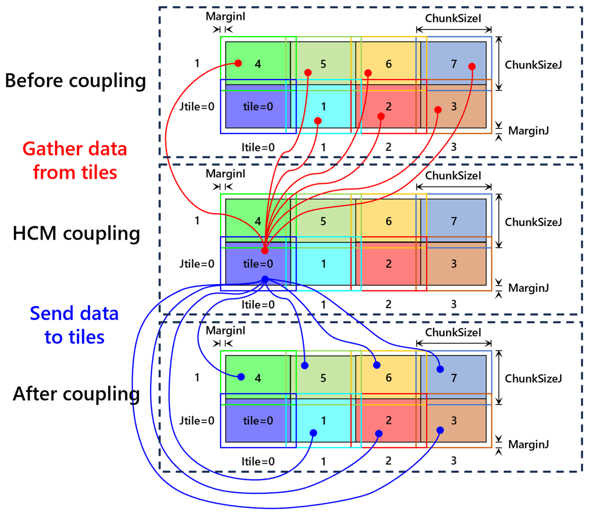
It is also important to highlight the coupler in the HCM_ROMS for the coupling process between the statistical atmospheric model and the ROMS model. Incorporating the statistical atmospheric model requires SST_inter from the entire ROMS domain. Therefore, data transmissions between different computing nodes are necessary for the coupling process. A coupler module based on the message passing interface (MPI) has been developed to facilitate the data transmissions in the HCM_ROMS (Fig. 5). With the coupler, the HCM_ROMS gathers the SST_inter from different computing nodes in the main computing node before coupling (red curves in Fig. 5). The main computing node then computes τ_inter and FWF_inter for the entire ROMS domain and sends the τ_inter and FWF_inter tiles to the corresponding computing nodes to drive the ROMS model (blue curves in Fig. 5). We have evaluated the performance of the coupler module at transferring data accurately and efficiently between the computing nodes (not shown). The successful construction of this coupler module lays the groundwork for the HCM_ROMS development.

Figure 5 Flow chart of the coupling process using MPI.

Besides the statistical atmospheric model, we also introduce a module in the HCM_ROMS to address the damping effects induced by the ocean–atmosphere heat transfer processes. The module based on a bulk approximate utilizes surface wind speed derived from the wind stress inversion to compute the turbulent heat transfer between the ocean and atmosphere, including both latent and sensible heat fluxes (Fairall et al., 1996):

$$\begin{array}{}\text{(1)}& {\displaystyle }& {\displaystyle }\mathrm{LH}={\mathit{\rho }}_{\mathrm{a}}{L}_{\mathrm{e}}{C}_{\mathrm{E}}{V}_{\mathrm{wg}}\left(q_{\mathrm{a}}-\mathrm{0.98}\times q_{\mathrm{sat}}\left(\mathrm{SST}\right)\right)\text{(2)}& {\displaystyle }& {\displaystyle }\mathrm{SH}={\mathit{\rho }}_{\mathrm{a}}{c}_{\mathrm{p}}{C}_{\mathrm{H}}{V}_{\mathrm{wg}}\left(T_{\mathrm{a}}-\mathrm{SST}\right),\end{array}$$

where LH and SH are latent and sensible heat fluxes, respectively; ρ_a is dry-air density; L_e is the latent heat of vaporization; c_p is the specific heat of dry air at constant pressure; C_E and C_H are the transfer coefficients for latent and sensible heat, respectively, set to $\mathrm{1.4}\times {\mathrm{10}}^{-\mathrm{3}}$ in this study; V_wg is the surface wind speed derived from the wind stress inversion ($V_{\mathrm{wg}}=\sqrt{\frac{\left|\mathit{\tau }\right|}{{\mathit{\rho }}_{\mathrm{a}}{C}_{\mathrm{D}}}}$), where |τ| is the magnitude of the wind stress vector and C_D is the transfer coefficient for drag, with a value of $\mathrm{1.7}\times {\mathrm{10}}^{-\mathrm{3}}$; T_a is air temperature; q_a is the atmospheric specific humidity; and q_sat(SST) is the saturated specific humidity at SST.

2.4 Experimental design

The HCM_ROMS model was first integrated for 60 years using the climatological atmospheric forcing (i.e., α_τ=0 and α_FWF=0) as the model's spinup. The spinup run was initialized with the January climatology of the Simple Ocean Data Assimilation Version 3 (SODA3) reanalysis with a horizontal resolution of 0.5°×0.5° (Carton et al., 2018). The climatological monthly SODA3 data also served as the lateral boundary conditions of sea surface height (SSH), currents, temperature, and salinity throughout the model integration. In terms of atmospheric forcing, the climatological monthly data for τ_clim, FWF_clim, and shortwave and longwave radiation were obtained from the Common Ocean Reference Experiment version 2 (COREv2) global air–sea flux dataset with a horizontal resolution of 1°×1° (Large and Yeager, 2009). The climatological monthly data for sea level pressure (SLP), surface air temperature, and surface air relative humidity utilized in calculating surface latent and sensible heat fluxes were sourced from the International Comprehensive Ocean–Atmosphere Data Set (ICOADS), with a horizontal resolution of 1°×1° (Freeman et al., 2017). It should be noted that the model's climatology in the following sensitivity experiments is calculated over the last 10 years of the spinup run.

After the spinup, we executed five sensitivity experiments, adjusting the α_τ values (α_τ=1.0, 1.3, 1.5, 1.7, and 2.0) to determine the optimal α_τ to reproduce sustainable interannual variabilities in the HCM_ROMS. These sensitivity experiments were integrated for 30 years and initiated through an “initial kick”, where the HCM_ROMS underwent forced integration with an imposed westerly wind anomaly lasting 8 months. The westerly wind anomaly during the initial kick was created using the statistical atmospheric model driven by an El Niño-like SSTA (Fig. 3), which was detected by the statistical atmospheric model but did not manifest in simulated SST. Subsequent anomalous conditions evolved solely through coupled ocean–atmosphere interactions within the HCM_ROMS. The FWF effects are not taken into account in this study and are set to α_FWF=0. This is because of the primary impact of the SSTA–τ_inter coupling on shaping the interannual variability associated with ENSO, while the SSTA–FWF_inter coupling, being capable of affecting the ENSO intensity, plays a secondary role (Gao et al., 2020). Further analysis of the FWF effects on the ENSO intensity in HCM_ROMS will be presented in Part 2 of this study (Yu et al., 2025).

3 Results and discussion

3.1 Statistical atmospheric model performance

We first examine the performance of the statistical atmospheric model at reproducing the ENSO-related interannual atmospheric forcing. Figure 6a shows the 40-year observed SSTA over the tropical zone of 5° S to 5° N from 1980 to 2020. The observed SSTA are derived from the monthly NOAA Extended Reconstructed SST (ERSST) version 5 dataset (Huang et al., 2017). We adopt ERSST in this subsection instead of using the NOAA OISST, which is used to construct the statistical atmospheric model in Sect. 2.1, to maintain the independence of the assessment. The observed SSTA shows a clear interannual characteristic related to ENSO, especially during the three major El Niño events of 1982/1983, 1997/1998, and 2015/2016, where the positive SSTA over the eastern Pacific can be above 2° C (Fig. 6a). The 40-year zonal wind stress anomaly and FWF anomaly over the tropical zone of 5° S to 5° N from 1980 to 2020 are shown in Fig. 6b and c, respectively. The monthly zonal wind stress anomaly and FWF anomaly are derived from the National Centers for Environmental Prediction and the National Center for Atmospheric Research (NCEP/NCAR) Reanalysis (Kalnay et al., 1996). During El Niño, the positive SSTA in the eastern Pacific corresponds to the eastward expansion of the anomalous westerly winds originating from the dateline, while in La Niña, abnormal easterly winds near the dateline emerge, leading to a cold SSTA east of the dateline (Fig. 6a and b). As for the FWF, the positive SSTA in the eastern Pacific during El Niño shifts the precipitation eastward to increase FWF in the eastern equatorial Pacific and reduces FWF in the western Pacific. Conversely, during La Niña, the FWF in the western equatorial Pacific increases, while the FWF in the eastern Pacific decreases (Fig. 6a and c).

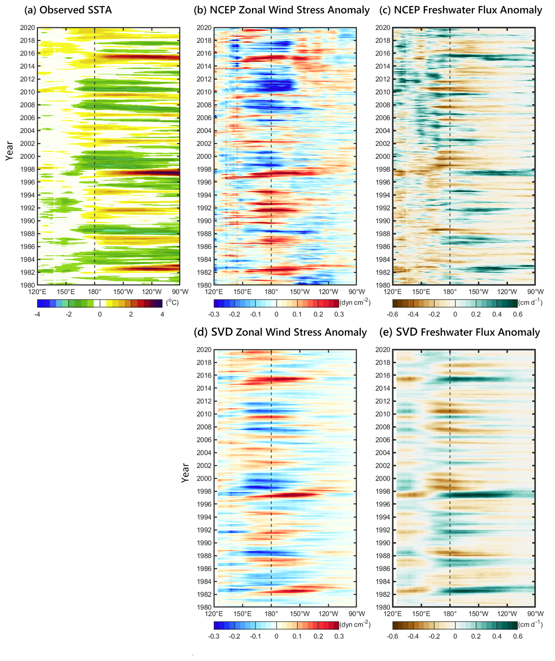
Figure 6 Hovmöller diagrams of observed (a) SSTA, (b) the zonal wind stress anomaly, and (c) the FWF anomaly over the tropical zone of 5° S to 5° N from 1980 to 2020. Panels (d) and (e) are the retrieved zonal wind stress anomaly and FWF anomaly using the statistical atmospheric model forced by the observed SSTA, respectively. The vertical dashed line indicates the dateline.

The retrieved zonal wind stress anomaly and FWF anomaly using the statistical atmospheric model forced by the observed SSTA from 1980 to 2020 are shown in Fig. 6d and e, respectively. During the three major El Niño events of 1982/1983, 1997/1998, and 2015/2016, the model replicates the observed anomalous westerly winds originating from the dateline (Fig. 6b and d). Additionally, in the five major La Niña events of 1988/1989, 1998/1999, 1999/2000, 2007/2008, and 2010/2011, the statistical atmospheric model also reproduces the abnormal easterly winds near the dateline, consistent with the NCEP/NCAR reanalysis (Fig. 6b and d). As for the FWF, the statistical atmospheric model reproduces the ENSO-related FWF anomaly dipole. The statistical atmospheric model produces a higher (lower) FWF in the eastern (western) equatorial Pacific during El Niño but the opposite occurs during La Niña (Fig. 6c and e). However, the statistical atmospheric model tends to underestimate the strength of interannual perturbations, especially for the wind stress, which may be due to the linear constraints in the SVD when dealing with nonlinear signals (Fig. 6b versus Fig. 6d). The statistical atmospheric model reproduces the observed interannual wind stress and FWF anomalies in phase (Fig. 6b–e). The correlation coefficient between the observed and simulated zonal wind stress anomalies is 0.62 (p<0.01), while the correlation coefficient for the observed and simulated FWF anomalies is 0.68 (p<0.01).

3.2 Simulated climatology in the ocean

The ROMS model performance at simulating the long-term mean and seasonal variability in ocean temperatures in the tropical Pacific was also assessed by comparing simulated ocean climatology with observational data. Here we note again that simulated ocean climatology in the study is defined as the long-term monthly mean averaged over the last 10 years of the spinup. This prolonged duration is necessary, as the ROMS model takes 30 to 40 years for simulated heat content in the upper 2000 m to reach equilibrium (not shown). To mitigate potential climate drift concerns arising from the model not reaching equilibrium, we employed a dataset covering the 51 to 60 years of the spinup run to calculate the model's climatology. The observed climatological monthly ocean temperature comprises averaged values from the World Ocean Atlas (WOA) 2023 dataset over the observation period of 1955 to 2022, with a horizontal resolution of 1°×1° (Locarnini et al., 2023).

Figure 7a shows the horizontal distribution of observed long-term mean SST over the tropical Pacific. It shows that the observed SST in the western Pacific warm pool, with an average value of 30° C is notably higher than in the surrounding area. Conversely, the cold-tongue region of the eastern equatorial Pacific shows distinct upwelling characteristics, leading to a lower average SST of only 24° C (Fig. 7a). The observed SST distribution matches the subsurface temperature structure changes along the Equator. The vertical cross-section of the observed temperature over the tropical zone of 5° S to 5° N along the Equator is shown in Fig. 7c. The higher SST observed in the western Pacific warm pool is attributed to the westward water transport in the equatorial Pacific, influenced by trade winds. The accumulated surface warm water in the western Pacific warm pool descends, leading to a deepening of the 20° C isotherm, reaching its maximum depth of 180 m west of the dateline. In the tropical eastern Pacific, the upwelling compensates for the trade-wind-induced westward surface transport, resulting in the ascent of deep cold water to the surface. The depth of the 20 °C isotherm progressively decreases away from the dateline, reaching its minimum depth of only 50 m along the coast of Peru at 90° W (Fig. 7c).

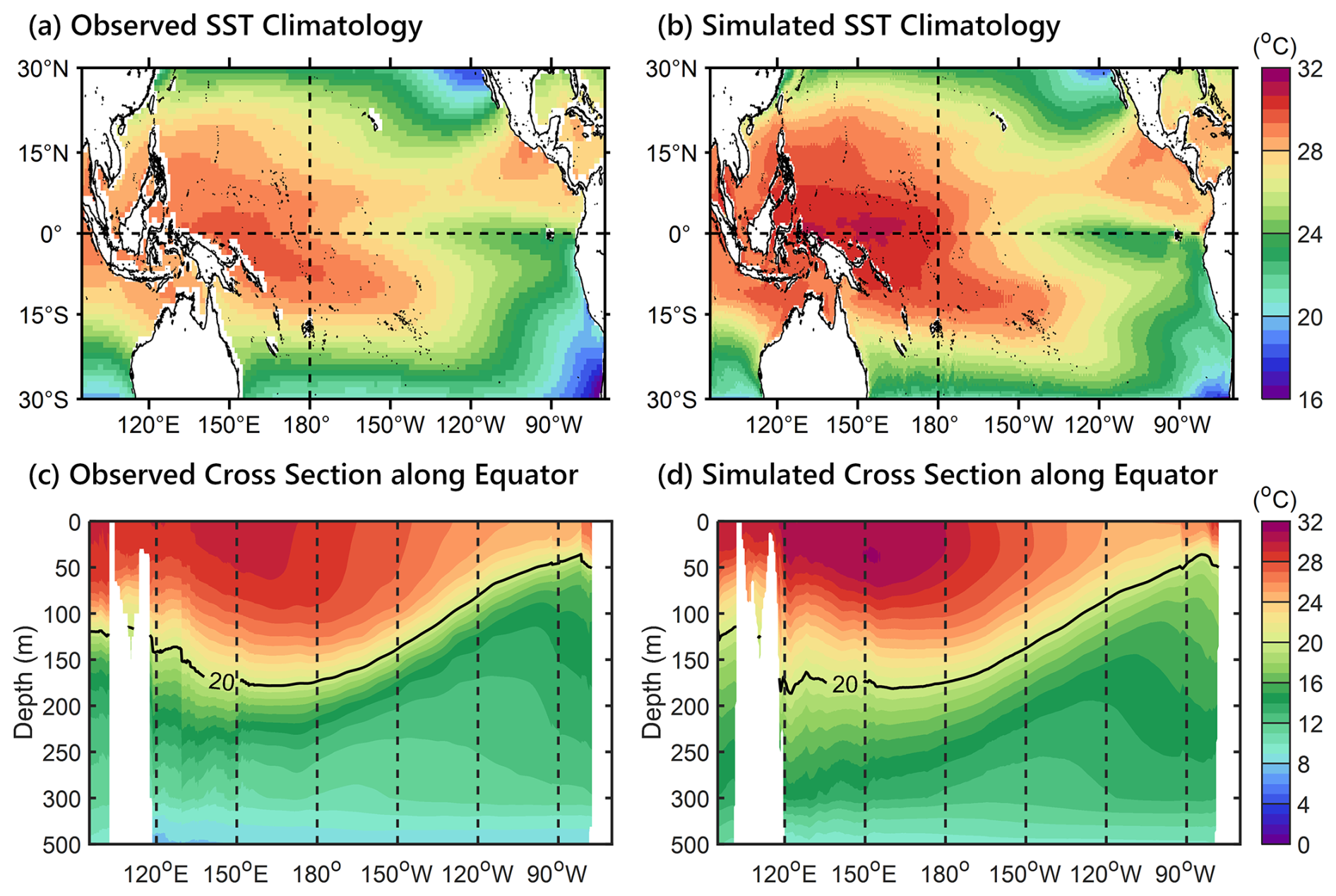
Figure 7 Horizontal distribution of (a) observed and (b) simulated long-term mean SST over the tropical Pacific. The (c) observed and (d) simulated vertical cross-section of the temperature along the Equator.

The simulated long-term mean SST distribution and vertical temperature structure along the Equator are shown in Fig. 7b and d, respectively. The ROMS model replicates the observed long-term mean temperature in the tropical Pacific that is indicated by the WOA data. The simulated western Pacific warm pool and the eastern Pacific cold tongue closely resemble those observed patterns (Fig. 7a and b). However, there is a notable overestimation of approximately 1 °C in the SST of the western Pacific warm pool by the ROMS model (Fig. 7b). This discrepancy may be attributed to the climatological atmospheric forcing adopted in the model, which excludes the influence of high-frequency stochastic atmospheric forcing signals such as tropical cyclones, westerly wind bursts, and the Madden–Julian Oscillation. The weaker climatological forcing, particularly from surface winds, leads to less vigorous vertical mixing in the ocean, potentially resulting in a warm bias in simulated SST. It is important to note that the modeled climatology driven by climatological forcing still exhibits some differences compared to the observed climatology, which refers to climatological results. The ROMS model reproduces the observed mean vertical temperature structure along the Equator (Fig. 7c and d). In the same as way as in the WOA observations, the simulated 20 °C isotherm deepens in the western equatorial Pacific, with a maximum depth of 180 m west of the dateline. Moving eastward, away from the dateline to the eastern equatorial Pacific, the simulated 20 °C isotherm depth decreases, reaching a minimum depth of 50 m along the coast of Peru at 90° W (Fig. 7c and d).

Figure 8 illustrates the seasonal climatology of observed and simulated SST in the tropical zone of 5° S to 5° N. West of the dateline, the observed SST exhibits a semiannual pattern. The highest temperature reaches30.5 °C in both May and November, while the lowest temperature, 29.5 °C, appears in February and August (Fig. 8a). This semiannual SST variation in the western equatorial Pacific is attributed to the sun's biannual crossing of the Equator, leading to corresponding semiannual changes in solar radiation. However, the observed SST shows a distinct annual cycle in the eastern Pacific, with the highest temperature of 28 °C in March and the lowest temperature of 23 °C in September (Fig. 8a). The annual SST variation in the eastern equatorial Pacific is driven by the effects of trade-wind-induced upwelling. The annual strengthening and weakening of the trade winds contribute to the annual SST changes in the eastern equatorial Pacific. Simulated seasonal SST climatology is shown in Fig. 8c. Despite the ROMS model overestimating the average SST in the western Pacific warm pool by 1 °C (Figs. 7b and 8c), it captures the observed semiannual SST variation in the western equatorial Pacific and the annual SST variation in the eastern equatorial Pacific. The annual variations in both observed and simulated SST are shown in Fig. 8b and d, respectively. The ROMS model replicates the observed seasonal SST changes, demonstrating an annual SST variation amplitude of ±3 °C in the eastern equatorial Pacific and a semiannual SST variation amplitude of ±0.5 °C in the western equatorial Pacific.

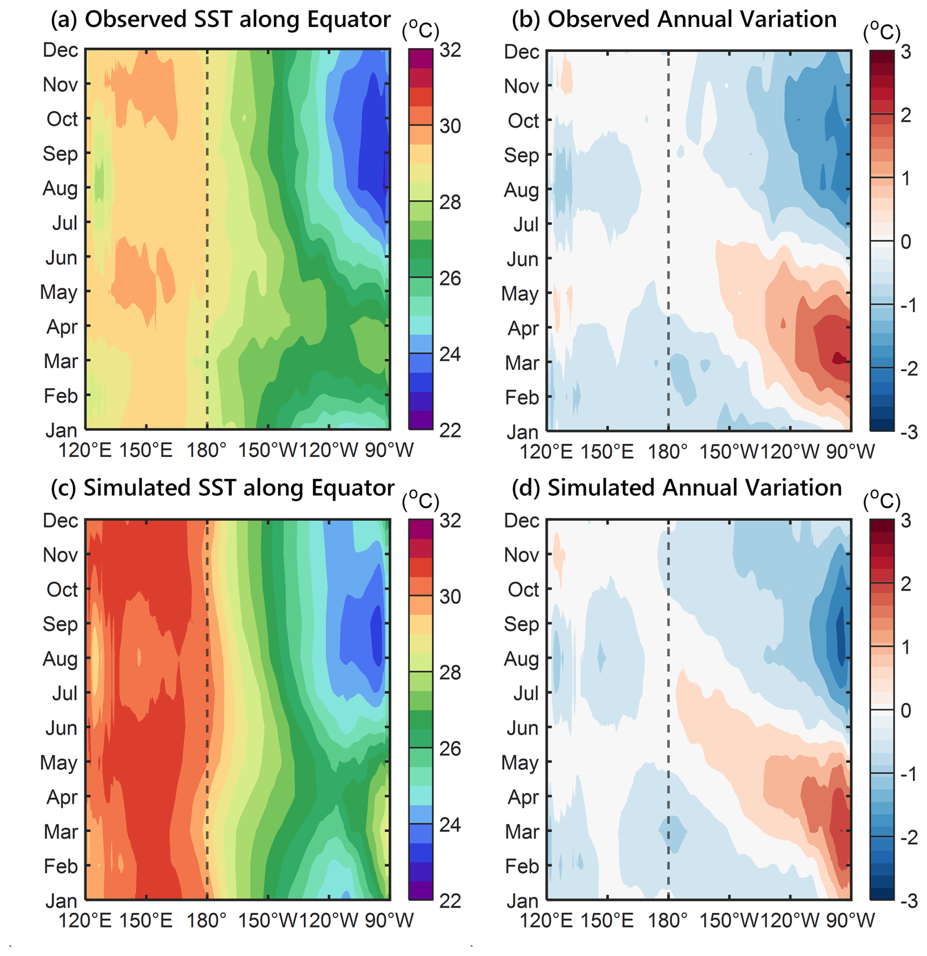
Figure 8 Hovmöller diagrams of (a) observed and (c) simulated seasonal SST along the Equator. Panels (b) and (d) are their annual variations.

3.3 Simulated interannual variability associated with ENSO

Figure 9 shows simulated Niño 3.4 index (SSTA averaged over the box region of 5° S to 5° N, 170 to 120° W) in the sensitivity experiments with different interannual wind stress coupling coefficients (α_τ=1.0, 1.3, 1.5, 1.7, and 2.0). Changes in the coupling coefficient, α_τ, lead to alterations in simulated interannual SST variability. The statistical atmospheric model tends to underestimate the strength of interannual disturbances due to the linear constraints within SVD (Fig. 6). Therefore, if the linear constraint effects are not counteracted, i.e., α_τ=1.0, the initial interannual oscillation signals generated during the initial kick will rapidly dissipate over 36 months (purple line in Fig. 9). This dissipation effect diminishes gradually as the coupling coefficient α_τ increases. When α_τ=1.3, the initial interannual oscillation signals gradually weaken and dissipate over 120 months (blue line in Fig. 9), whereas at α_τ=1.5, the initial interannual oscillation signals can be consistently sustained, exhibiting a steady quasi-3-year cycle (thick black line in Fig. 9). However, when α_τ exceeds 1.5, with increases in the coupling coefficient α_τ, the simulated interannual oscillations become unstable. At α_τ=1.7, the amplitude of simulated Niño 3.4 index increases to 2.8 °C, exceeding the initial amplitude of 1.8 °C (red line in Fig. 9). Meanwhile, at α_τ=2.0, the period of the simulated interannual SST variability changes and the stable quasi-3-year oscillations give way to irregular quasi-biennial oscillations, which are characterized by alternating strong and weak biennial oscillations over a 4-year period (orange line in Fig. 9). The above evidence suggests a substantial relation between the modeled interannual SST and the coupling coefficient α_τ. Given that the optimal α_τ=1.5 produces sustainable interannual variabilities in the HCM_ROMS, subsequent analysis is based on the experiment with the interannual wind stress coupling coefficient α_τ set to 1.5.

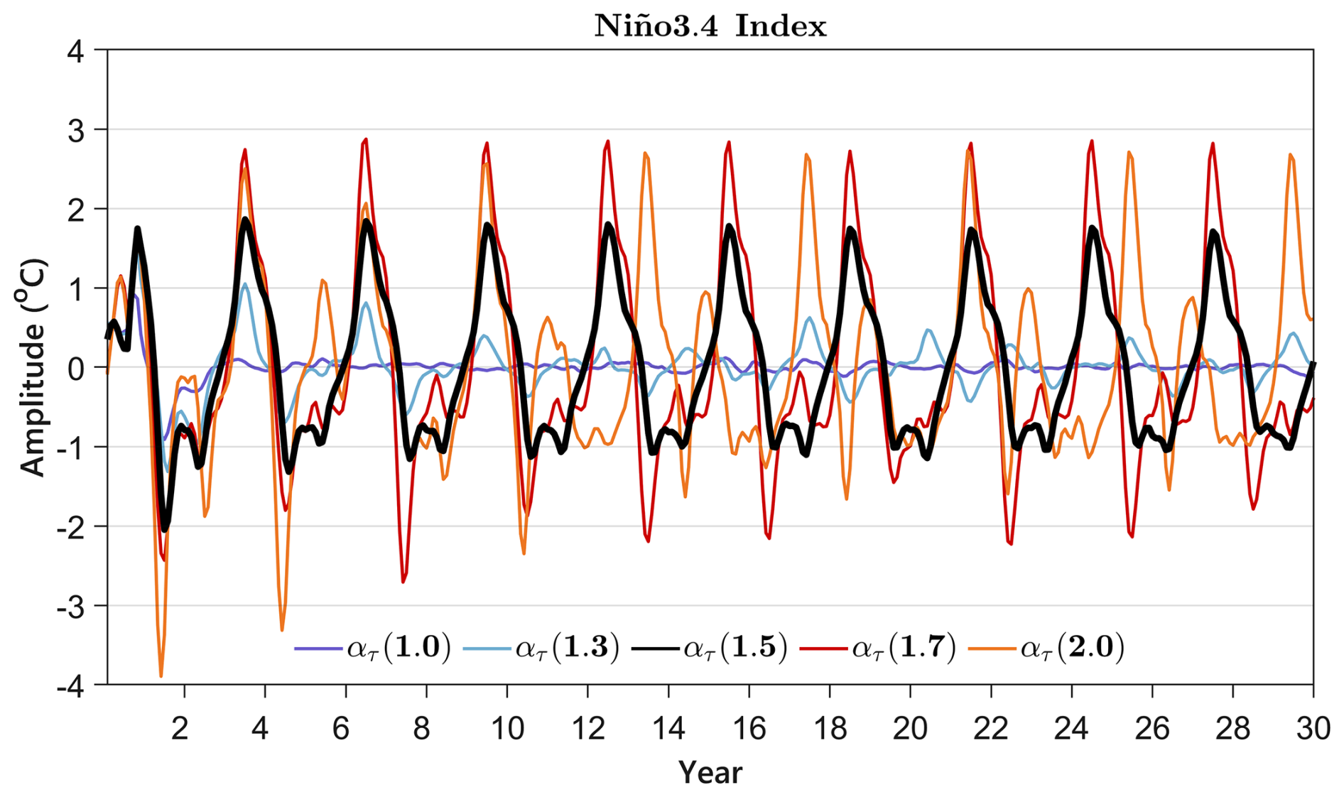
Figure 9 Simulated Niño 3.4 index in the sensitivity experiments with different interannual wind stress coupling coefficients. The purple line is for α_τ=1.0, the blue line for α_τ=1.3, the black line for α_τ=1.5, the red line for α_τ=1.7, and the orange line for α_τ=2.0.

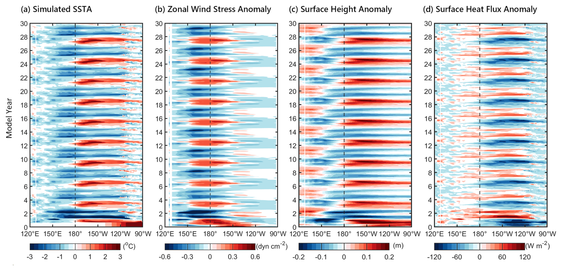
Figure 10 Hovmöller diagrams of simulated (a) SSTA, (b) the zonal wind stress anomaly, (c) the surface height anomaly, and (d) the surface heat flux anomaly averaged over the tropical zone of 5° S to 5° N along the Equator for the sensitivity experiment with α_τ=1.5.

The Hovmöller diagrams of simulated SSTA, zonal wind stress anomaly, surface height anomaly, and surface heat flux anomaly for the sensitivity experiment with α_τ=1.5 are shown in Fig. 10a–d, respectively. These anomalies are averaged over the tropical zone of 5° S to 5° N along the Equator. During the first-8-month initial kick, the prescribed idealized El Niño-like SSTA (Fig. 3) drives the statistical atmospheric model to generate abnormal westerly winds east of the dateline (Fig. 10b). The anomalous westerly winds persist for 8 months, transporting surface warm water eastward and increasing the sea surface height in the eastern equatorial Pacific (Fig. 10c). The eastward water transport induced by anomalous westerly winds during the initial kick drives the ROMS model to produce an initial positive SSTA of 2 °C east of the dateline (Fig. 10a). The initial positive SSTA in the eastern Pacific subsequently triggers the ENSO cycle in the HCM_ROMS. Specifically, simulated ENSO in the HCM_ROMS shows the alternating occurrence of El Niño with a positive SSTA of 2 °C and La Niña with a negative SSTA of −1 °C, maintaining a stable quasi-3-year cycle (Fig. 10a). During simulated El Niño and La Niña, the anomalous westerly wind stress anomaly of 0.3 dyn cm⁻² and easterly wind stress anomaly of −0.3 dyn cm⁻² emerge around the dateline, the same as in the observations (Figs. 6b and 10b). The abnormal westerly and easterly winds that occur near the dateline during El Niño and La Niña strengthen the eastward and westward equatorial water transport, contributing to the SSTA evolution associated with El Niño and La Niña, respectively (Fig. 10c). In addition, the surface heat flux anomaly with an amplitude of ±60 W m⁻² dampens the positive and negative SSTAs associated with simulated El Niño and La Niña (Fig. 10d).

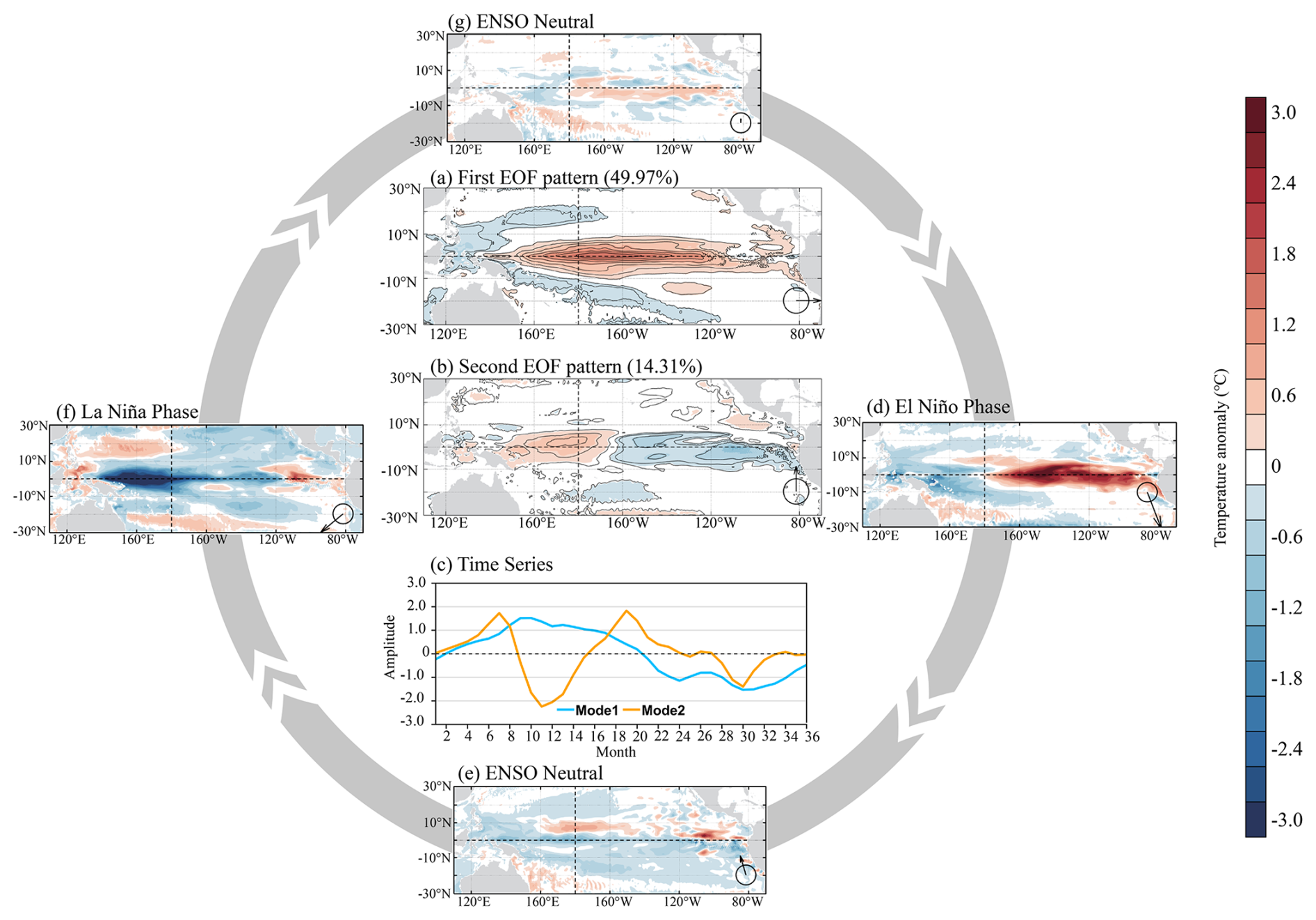
Figure 11 Distribution of the (a) first and (b) second empirical orthogonal function (EOF) patterns of simulated SSTA in the sensitivity experiment with α_τ=1.5 and (c) their time coefficients. Panels (d)–(g) are the spatial patterns of SSTA over the ENSO cycle. Vectors at the bottom right of panels (a, b) and (d)–(g) show the associated principal components (PCs). The abscissa is PC1, the ordinate is PC2, and the arrow length is the magnitude in the PC1–PC2 space (an arrow magnitude of 1 is indicated by the circles).

We note that incorporating the SSTA–τ_inter coupling in the HCM_ROMS can reduce the average SST in the western Pacific warm pool by 0.6–0.8 °C (Fig. 10a). This helps alleviate the overestimation of SST during the model spinup due to the weaker climatological atmospheric forcing adopted in the model (Figs. 7 and 8), implying that ENSO may play a specific role in regulating the average state of the western Pacific warm pool and Pacific western boundary currents (Hu et al., 2015). Although it is not the focus of this study, the newly developed HCM_ROMS may serve as a potential tool to investigate the ENSO impacts on the western Pacific warm pool and Pacific western boundary currents in the future.

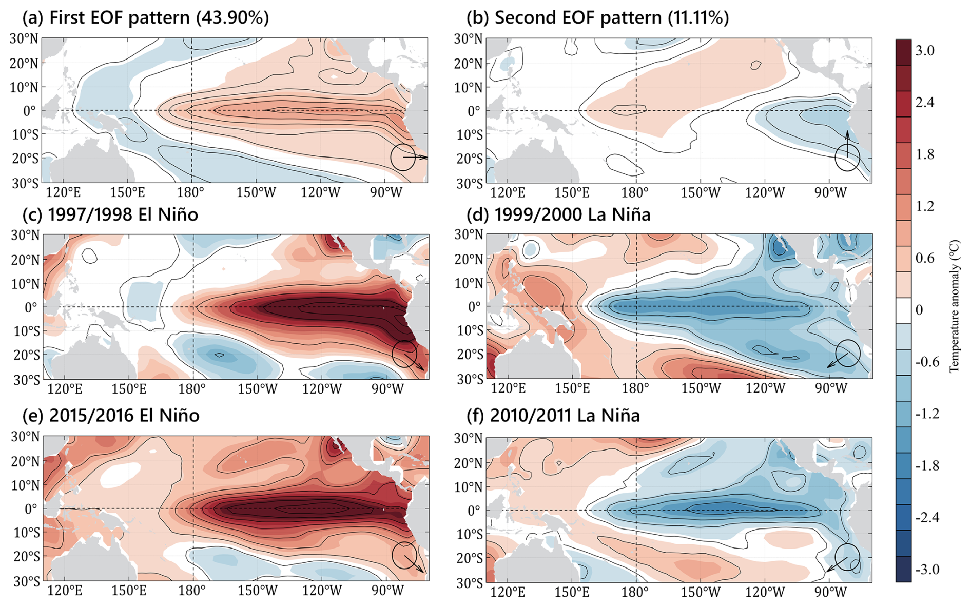
Figure 12 Distribution of the (a) first and (b) second EOF patterns of observed SSTA and spatial patterns of SSTA during the (c) 1997/1998 El Niño, (d) 1999/2000 La Niña, (e) 2015/2016 El Niño, and (f) 2010/2011 La Niña.

To assess simulated ENSO in the HCM_ROMS following the method documented by Timmermann et al. (2018), we conducted an empirical orthogonal function (EOF) analysis of simulated SSTA from 9 to 30 years (three cycles after the initial kick) in the sensitivity experiment with α_τ=1.5. It shows that the leading EOF (mode 1), contributing 49.97 % to the variance, has a classic El Niño pattern (Fig. 11a) and exhibits variability on a quasi-3-year timescale (blue line in Fig. 11c). The second EOF (mode 2), contributing 14.31 % to the variance, presents a tropical east–west zonal dipole (Fig. 11b) with enhanced variability on a 1.5-year timescale (orange line in Fig. 11c). The interplay between the first and second EOFs captures the spatial and temporal evolution of simulated ENSO (Fig. 11d–g). The second EOF serves as an amplifier for the simulated warming anomaly in the equatorial eastern Pacific during El Niño, emphasizing the impacts of the Bjerknes feedback. Specifically, when simulated El Niño onset (time coefficient of mode 1 surpasses 1), the time coefficient of mode 2 undergoes a transition from positive to negative, reaching its minimum of −2 1 month after the time coefficient of mode 1 achieves its maximum of 1.5 (Fig. 11c). The opposite-sign pattern of mode 2 corresponds to the process wherein the Bjerknes feedback induces warming in the eastern equatorial Pacific and cooling in the western equatorial Pacific during El Niño, implying that the second EOF may represent the effects of the Bjerknes feedback (Fig. 11b). However, this amplifying effect of the second EOF was absent during simulated La Niña. Both mode 1 and mode 2 shared the same negative sign during the onset of simulated La Niña (time coefficient of mode 1 falling below −1; Fig. 11c), with mode 2 acting as a damper rather than amplifying the cooling in the eastern equatorial Pacific (Fig. 11f). This explains the asymmetry between simulated El Niño and La Niña in the HCM_ROMS, where the amplitude of the simulated Niño 3.4 index during El Niño surpasses that during La Niña (Figs. 9 and 10a).

As a comparison, the first and second EOFs of the observed SSTA from 1980 to 2020 are shown in Fig. 12a and b, respectively. Notably, the simulated second EOF in HCM_ROMS fails to capture the influence of the Victoria mode compared to the observations (Figs. 11b and 12b). This discrepancy may arise from the limited model domain of the tropical Pacific (30° S to 30° N; Fig. 3) used in this study, which results in the absence of extratropical processes in the HCM_ROMS (Ding et al., 2017, 2019). Nevertheless, the EOFs of observed and simulated SSTA still share certain similarities. The first EOF of observed SSTA shows an El Niño pattern with a variance contribution of 43.90 % (Fig. 12a) and the second EOF presents a tropical east–west zonal dipole with a variance contribution of 11.11 % (Fig. 12b). In addition, the observed first and second EOFs have similar configurations (phase configuration of mode 1 and mode 2, the phase vectors shown in Fig. 12c–f) during El Niño and La Niña compared to simulated EOFs (Fig. 11d and f). During the 1997/1998 and 2015/2016 El Niño events, the observed SSTAs feature positive mode 1 and negative mode 2 (phase vectors are in the fourth quadrant; Fig. 12c and e), while during the 1999/2000 and 2010/2011 La Niña events, they exhibit negative mode 1 and mode 2 (phase vectors are in the third quadrant; Fig. 12d and f), highlighting the asymmetrical role of mode 2 during El Niño and La Niña. While the HCM_ROMS depicts the distinct functions of the second EOF during simulated El Niño and La Niña (Fig. 11c, d, and f), complex factors may contribute to the mechanisms involved, which surpass the scope of this study. We currently abstain from further investigation into details, merely speculating that the asymmetry in the Bjerknes feedback during El Niño and La Niña, possibly coupled with extratropical processes, could affect these patterns.

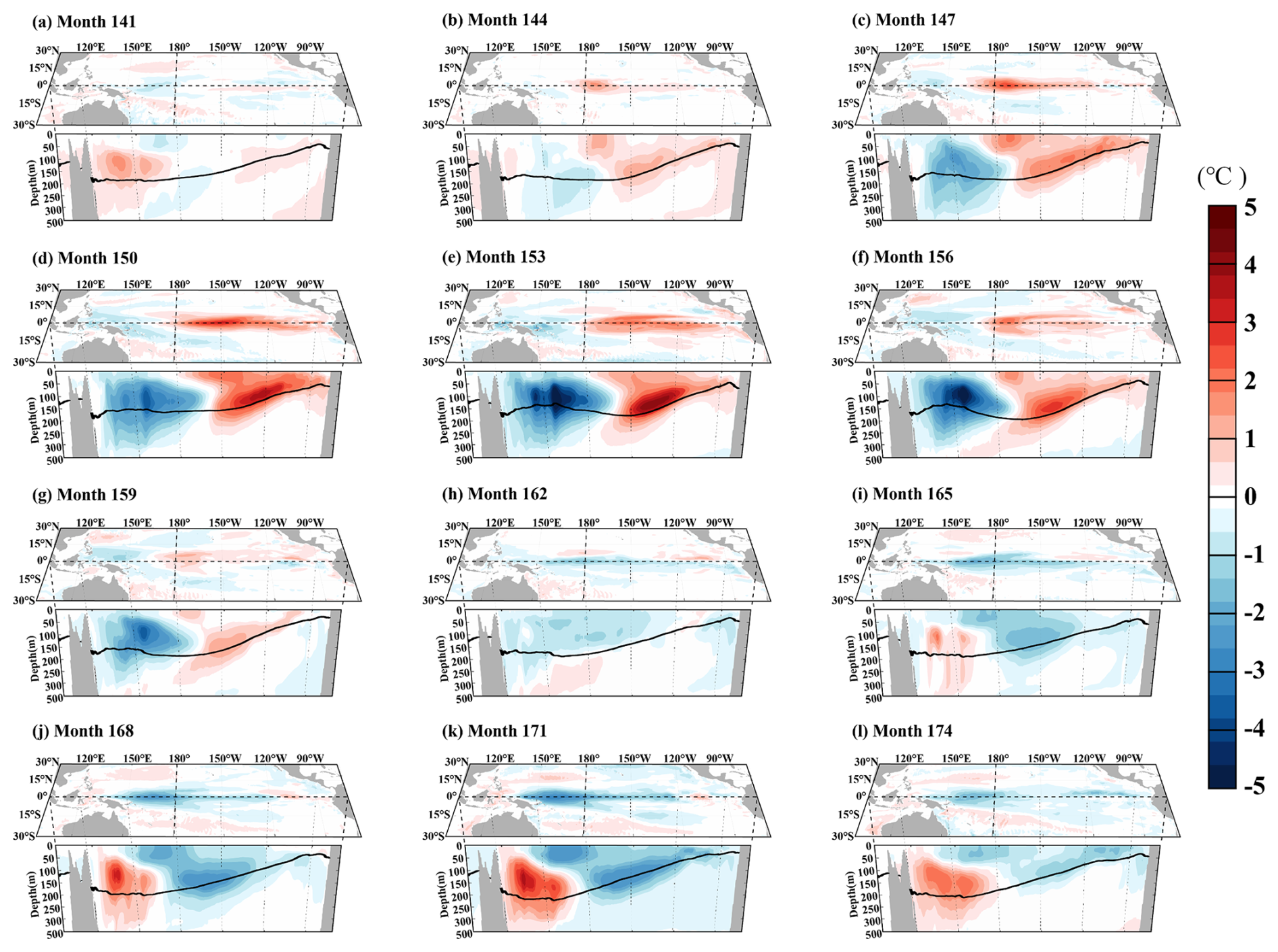
Figure 13 Three-dimensional temperature anomalies over the simulated ENSO cycle from month 141 to 174 in the sensitivity experiment with α_τ=1.5.

In addition to simulated interannual SSTA, the HCM_ROMS has the advantage of simulating the subsurface temperature changes associated with ENSO. Figure 13 shows the evolution of 3D temperature anomalies over a complete ENSO cycle spanning month 141 to 174 in the sensitivity experiment with α_τ=1.5. It shows that a subsurface warm anomaly forms along the 20 °C isotherm (black contour in Fig. 13) east of the dateline during simulated El Niño onset (Fig. 13a and b). This subsurface warming intensifies with simulated El Niño growth (Fig. 13b and c) and reaches its maximum of 3–4 °C, exceeding the surface warming of 2 °C during the mature stage of simulated El Niño (Fig. 13d and e). At the same time, a subsurface cooling of −3 to −4 °C forms along the 20 °C isotherm west of the dateline (Fig. 13c–e). When simulated El Niño decays, the subsurface cooling west of the dateline propagates eastward along the 20 °C isotherm, gradually counteracting the subsurface warming in the eastern equatorial Pacific (Fig. 13f–h), while in the simulated onset of La Niña, the subsurface cooling east of the dateline intensifies (Fig. 13i), reaching a peak cold anomaly of −2 °C during the mature stage of simulated La Niña (Fig. 13j and k). Subsurface warming of 3–4 °C along the 20 °C isotherm west of the dateline emerges during simulated La Niña (Fig. 13i–k). The subsurface warming west of the dateline offsets La Niña-related subsurface cooling in the equatorial eastern Pacific when simulated La Niña decays (Fig. 13l). The aforementioned subsurface temperature changes associated with simulated ENSO in HCM_ROMS closely align with the empirical observations (see Fig. 1 in Timmermann et al., 2018), validating the HCM_ROMS model's ability to depict the intricate 3D temperature structure changes during ENSO evolution.

3.4 Budget analysis of 3D evolution of simulated ENSO

To better understand the 3D temperature changes related to simulated ENSO in the HCM_ROMS, a postprocessing heat budget analysis for the interannual temperature anomaly has been developed in this study. The temperature evolution within the ROMS model is governed by the advective–diffusive equation:

$$\begin{array}{}\text{(3)}& \underset{\mathrm{T}\mathrm{\_}\mathrm{rate}}{\underbrace{{\displaystyle \frac{\partial T}{\partial t}}}}=\underset{\mathrm{T}\mathrm{\_}\mathrm{adv}}{\underbrace{-\mathit{V}\mathrm{\nabla }T}}+\underset{\mathrm{T}\mathrm{\_}\mathrm{hdif}}{\underbrace{{\mathrm{\nabla }}_{\mathrm{h}}\cdot \left(K_{\mathrm{h}}{\mathrm{\nabla }}_{\mathrm{h}}T\right)}}+\underset{\mathrm{T}\mathrm{\_}\mathrm{vdif}}{\underbrace{{\displaystyle \frac{\partial }{\partial z}}\left(K_{\mathrm{v}}{\displaystyle \frac{\partial t}{\partial z}}\right)}}+\underset{\mathrm{T}\mathrm{\_}\mathrm{solar}}{\underbrace{{\displaystyle \frac{Q_{\mathrm{R}}}{{\mathit{\rho }}_{\mathrm{w}}{C}_{\mathrm{p}}}}}},\end{array}$$

where T is the potential temperature; V is the current vector; ∇ is the gradient operator; ∇_h is the horizontal gradient operator; K_h and K_v are the horizontal and vertical diffusivities, respectively; ρ_w is the seawater density; C_p is the specific heat of seawater at constant pressure; and $Q_{\mathrm{R}}=\frac{\partial F_{\mathrm{S}}}{\partial z}$ is the radiative heating rate, where F_S is the solar radiative heat flux in the ocean due to solar radiation penetration. The diagnostic terms T_rate, T_adv, T_hdif, T_vdif, and T_solar in Eq. (3) represent the temperature tendency, total (horizontal + vertical) advection, horizontal diffusion, vertical diffusion, and solar radiative heating, respectively. The total advection term T_adv includes both horizontal processes, e.g., the influence of the equatorial currents, and vertical processes, e.g., the downwelling Kelvin waves triggered by the westerly wind anomalies. We do not separate the total advection effect into the horizontal and vertical components due to the interconnected nature of these two terms on the monthly timescale, as such a separation does not yield additional interpretability (not shown). The above diagnostic terms are direct outputs of the HCM_ROMS, which can greatly reduce the budget error.

We note that the impacts of longwave radiation and latent and sensible heat fluxes on the temperature changes in the ROMS model are also included in Eq. (3) because these surface heat fluxes serve as the upper boundary condition of the vertical diffusion term T_vdif,

$$\begin{array}{}\text{(4)}& {\left.K_{\mathrm{v}}{\displaystyle \frac{\partial T}{\partial z}}\right|}_{z=\mathit{\zeta }}={\displaystyle \frac{\mathrm{LW}+\mathrm{LH}+\mathrm{SH}}{{\mathit{\rho }}_{\mathrm{w}}{C}_{\mathrm{p}}}},\end{array}$$

where ζ is the sea surface height; LW is the longwave radiation flux; and LH and SH are the latent and sensible heat fluxes calculated by the bulk heat flux formulas (Eqs. 1 and 2), respectively.

The ENSO-related interannual temperature changes in the HCM_ROMS can be diagnosed using the following interannual form of the budget equation:

$$\begin{array}{}\text{(5)}& \left[\mathrm{T}\mathrm{\_}\mathrm{rate}\right]=\left[\mathrm{T}\mathrm{\_}\mathrm{adv}\right]+\left[\mathrm{T}\mathrm{\_}\mathrm{hdif}\right]+\left[\mathrm{T}\mathrm{\_}\mathrm{vdif}\right]+\left[\mathrm{T}\mathrm{\_}\mathrm{solar}\right],\end{array}$$

where [ ] denotes the interannual operator, which means that the simulated values subtract their climatological mean. The climatological mean of the budget terms utilized in Eq. (5) are averaged to the long-term monthly mean over the last 10 years of the spinup. We do not show [T_solar] in this study, as the solar radiative heat flux in the ocean is calculated by an empirical irradiance absorption scheme with fixed attenuation depth (see Table 2 in Paulson and Simpson, 1977) and the solar radiation forcing at the sea surface is derived from the climatology monthly COREv2 data and thus has no interannual variability.

During the simulated onset of El Niño (months 141–153; Fig. 13a–e), the [T_rate] shows a positive temperature tendency of $\mathrm{2}\times {\mathrm{10}}^{-\mathrm{7}}$° s⁻¹ to the east of the dateline, with a maximum warming rate of $\mathrm{3}\times {\mathrm{10}}^{-\mathrm{7}}$° s⁻¹ at a depth of 150 m between 150 and 120° W (Fig. 14a), reflecting the 3D temperature changes. The positive [T_rate] east of the dateline leads to an increase in the upper-ocean temperature, deepening the mean depth of the 20 °C isotherm (solid red line) by 20 m in the eastern Pacific compared to the simulated climatology (solid gray line; averaged over the same month of the year during the last 10 years of the spinup). Meanwhile, a negative temperature tendency of $-\mathrm{2}\times {\mathrm{10}}^{-\mathrm{7}}$° s⁻¹ is obtained west of the dateline, resulting in additional cooling and reducing the mean depth of the 20 °C isotherm by 20 m west of the dateline (Fig. 14a). The budget analysis indicates that the [T_rate] pattern in Fig. 14a is primarily influenced by the advection effect [T_adv], wherein the abnormal westerly winds around the dateline (Fig. 10b) during the onset of El Niño induce anomalous eastward advection, leading to the warming (cooling) to the east (west) of the dateline (Fig. 14e). Simulated warming in the subsurface layer exceeding that of the surface during El Niño (Fig. 13a–e) is due to the vertical diffusion effect [T_vdif]. Since the surface heat flux damping during El Niño works to reduce the SST (Fig. 10d), vertical mixing transports the damping effects from the surface to the deeper layers, partly counteracting the warming in the upper ocean (Fig. 14i).

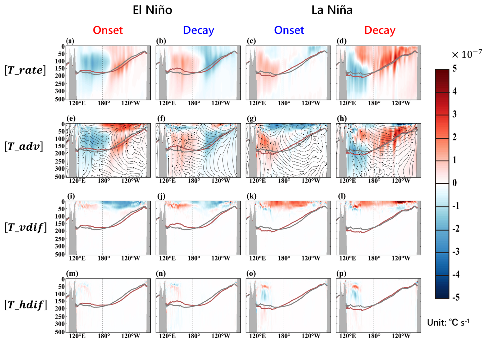
Figure 14 Vertical cross-section plots of the (a–d) tendency, (e–h) advection, (i–l) vertical diffusion, and (m–p) horizontal diffusion of the interannual temperature budget equation (Eq. 5). The streamlines in panels (e)–(h) represent the averaged flow field during the budget calculation.

In the decay phase of simulated El Niño (months 153–162; Fig. 13e–h), both advection and vertical diffusion effects play constructive roles in shaping the dipole-type temperature changes (Fig. 14b, f and g). With the reduction in abnormal westerly winds during El Niño decay (Fig. 10b), prevailing easterly winds east to the dateline (i.e., trade winds) facilitate westward water transport in the equatorial Pacific. The advection effect [T_adv] counteracts the accumulated subsurface warming in the eastern Pacific by transporting warm water to the western Pacific. The descent of warm water around the dateline raises the subsurface temperature in the western Pacific (Fig. 14f). As for the vertical diffusion effect, due to the SST still being warmer than normal during El Niño decay, the surface heat flux and thus the vertical diffusion effect [T_vdif] continue to cool the upper ocean (Figs. 10d and 14j).

As for the La Niña period, the budget analysis suggests that the advection and vertical diffusion effects play similar roles during La Niña onset (Fig. 14c, g, and k) and decay (Fig. 14d, h, and l) but with opposite signs compared to those in the El Niño period. The horizontal diffusion effect [T_hdif] is not discussed, as it only appears in the subsurface west of 150° E and has a limited impact on ENSO evolution (Fig. 14m–p).

4 Conclusions

In this study, we developed a new HCM using the advanced ocean model ROMS (HCM_ROMS) to simulate ENSO. Within the HCM_ROMS framework, the ROMS model was coupled with an SVD-based statistical atmospheric model, capturing interannual atmospheric perturbations, including wind stress and FWF anomalies (i.e., τ_inter and FWF_inter). A turbulent heat flux module employing bulk approximation and wind-stress-inverse wind speed was incorporated into the HCM_ROMS to address the damping effects of surface heat flux on ENSO dynamics. We executed five sensitivity experiments, adjusting the interannual wind stress coupling coefficient α_τ from 1.0 to 2.0 to determine the optimal α_τ to reproduce sustainable interannual variabilities in the HCM_ROMS. A postprocessing budget scheme for the interannual temperature anomaly was also developed to analyze the processes responsible for ENSO-related 3D temperature changes.

We first examined the performance of the statistical atmospheric model at reproducing the ENSO-related interannual forcing. The retrieved zonal wind stress and FWF anomalies using the statistical atmospheric model forced by the observed SSTA from 1980 to 2020 were compared with the observed values from the NCEP/NCAR reanalysis. The SVD-based statistical atmospheric model replicates the observed anomalous westerly winds originating from the dateline during the major El Niño events of 1982/1983, 1997/1998, and 2015/2016 and the abnormal easterly winds near the dateline in the major La Niña events of 1988/1989, 1998/1999, 1999/2000, 2007/2008, and 2010/2011. The statistical atmospheric model also reproduces the ENSO-related FWF anomaly dipole during El Niño and La Niña. The correlation coefficient between the observed and simulated zonal wind stress anomalies is 0.62 (p<0.01), and the correlation coefficient for the observed and simulated FWF anomalies is 0.68 (p<0.01).

The ROMS model performance at simulating the mean and seasonal temperatures in the tropical Pacific was also assessed by comparing simulated climatology with the WOA observations. Although there is a notable overestimation of 1 °C in the mean SST of the western Pacific warm pool during the model spinup, possibly due to the weaker climatological forcing adopted in the model, the ROMS model replicates the observed SST distribution and the vertical temperature structures along the Equator. The simulated 20 °C isotherm deepens in the western equatorial Pacific, with a maximum depth of 180 m west of the dateline. The simulated 20 °C isotherm depth decreases away from the dateline, reaching a minimum depth of 50 m along the coast of Peru at 90° W. The ROMS model captures the observed semiannual SST variation of ±0.5 °C in the western equatorial Pacific and the annual SST variation of ±3°C in the eastern equatorial Pacific. The semiannual SST variation in the western equatorial Pacific is attributed to the sun's biannual crossing of the Equator, while the annual SST variation in the eastern equatorial Pacific is driven by the effects of trade-wind-induced upwelling.

Sensitivity experiments with different α_τ values indicate that the optimal α_τ=1.5 can produce sustainable interannual variabilities in the HCM_ROMS. With the α_τ set to 1.5, HCM_ROMS produces a stable quasi-3-year ENSO cycle following the initial 8-month model kick process. The simulated ENSO cycle is characterized by the alternating occurrence of El Niño events with SST anomalies of 2 °C and La Niña events with SST anomalies of −1 °C. During simulated El Niño and La Niña, the anomalous westerly wind stress anomaly of 0.3 dyn cm⁻² and easterly wind stress anomaly of −0.3 dyn cm⁻² emerge around the dateline. A surface turbulent heat flux anomaly of ±60 W m⁻² appears in the eastern Pacific to dampen the positive and negative SSTAs associated with simulated El Niño and La Niña, respectively.

EOF analysis was utilized to evaluate the HCM_ROMS performance at replicating ENSO-related interannual variability. It revealed that mode 1 of simulated SSTA, accounting for 49.97 % of the variance, displays a classic El Niño pattern and demonstrates variability on a quasi-3-year timescale. Mode 2, explaining 14.31 % of the variance, depicts a tropical east–west zonal dipole with heightened variability on a 1.5-year timescale. However, the simulated mode 2 in HCM_ROMS fails to capture the influence of the Victoria mode, possibly due to the absence of extratropical processes from the limited model domain of the tropical Pacific. The EOFs of observed and simulated SSTA share certain similarities, including close variance contributions and similar phase configurations. Mode 2 represents the Bjerknes feedback and serves as an amplifier during El Niño but acts as a damper during La Niña. The distinct functions of mode 2 explain the asymmetry between simulated El Niño and La Niña in the HCM_ROMS.

The HCM_ROMS reproduces the 3D temperature changes during ENSO evolution, revealing that the most significant temperature anomalies occur beneath the surface at 150 m. The budget analysis indicates that the interannual temperature tendency [T_rate] is primarily influenced by the advection effect [T_adv] driven by interannual wind stress. The vertical diffusion effect [T_vdif] also contributes to the formation of subsurface anomaly maxima. However, the primary role of [T_vdif] is not to amplify cold or warm anomalies within the subsurface layer. Instead, it works to diminish these anomalies within the upper ocean due to the damping effects of turbulent heat flux. Anomalies induced by advection effects in the upper ocean are counteracted by the vertical diffusion effect, resulting in the appearance of subsurface maxima.

The newly developed HCM_ROMS provides an effective tool to represent and simulate ENSO in the tropical Pacific climate system. In this study, we focus on the SSTA–τ_inter coupling, while excluding the FWF effects by setting α_FWF=0. The SSTA–FWF_inter coupling also impacts ENSO and can be flexibly included in the HCM_ROMS. Further exploration of the FWF effects using the HCM_ROMS as a tool will be presented in a future study. In addition, the ROMS model has advantages when modeling multiscale ocean physical and biogeochemistry processes, such as mesoscale eddies, tropical instability waves, and ocean-biology-induced heating effects. The interactions between multiscale processes and ENSO will also be a focal point of future research utilizing the HCM_ROMS as a flexible modeling tool.