Comprehensive evaluation of iAMAS (v1.0) in simulating Antarctic meteorological fields with observations and reanalysis

Regular latitude-longitude grids in global simulations encounter polar singularities in the Arctic and Antarctic regions. In contrast, unstructured meshes have the potential to overcome this issue; however, so far, the performance of unstructured meshes in polar areas has barely been investigated. This study investigates the efficacy of unstructured meshes over Antarctica using the integrated Atmospheric Model Across Scales (iAMAS, v1.0) with multi-source observations. Four mesh configurations of the iAMAS model were assessed, varying in resolution (120, 60, 16, and 4 km) over the Antarctic region. The study evaluates the performance of the iAMAS simulation for both the surface layer and the upper meteorological fields (temperature, pressure, specific humidity, and wind speed), comparing simulations with data from the fifth-generation ECMWF reanalysis (ERA5) and measurements from automatic weather stations and radiosondes. The results indicate that the iAMAS model does not exhibit the polar singularity issue observed in ERA5, where the ERA5 with regular latitude-longitude grids significantly underestimates wind speeds at the polar grid center. In the relatively flat region of East Antarctica, all four iAMAS experiments at various resolutions demonstrate comparable and even superior performance in simulating temperature and wind speed compared to ERA5. In regions with complex terrain, such as near the Transantarctic Mountains, the iAMAS model (particularly at coarse grid resolutions like 120 km) exhibits a cold bias and stronger wind speeds, consistent with biases identified in other Antarctic simulations using regional models. In particular, mesh refinement at 4 km in complex terrains significantly enhances iAMAS's accuracy in simulating the meteorological fields for both the surface layer and upper atmosphere, suggesting that a grid resolution of 4 km (or even higher) is optimal in such regions. In contrast, in flatter areas, such as the high East Antarctic Plateau, increases in grid resolution yield minimal improvements in simulation accuracy, and a 60 km grid resolution appears sufficient.

1 Introduction

The Antarctic continent is the highest, driest, and coldest region on Earth, providing a unique environment for testing atmospheric models under extreme conditions. Furthermore, this distinctive environment facilitates a range of sophisticated scientific experiments, including ice-core records of climate properties (Petit et al., 1999), assessments of Antarctic contributions to future sea-level rise (Golledge et al., 2015), investigations into the role of ice sheets in the global carbon cycle (Wadham et al., 2019), and studies on Antarctic ozone holes (Kessenich et al., 2023). Additionally, increases in surface temperature are expected to be amplified in polar regions (Clem et al., 2020; Douville, 2023), and the effects of Antarctic amplification have garnered significant attention (Wang et al., 2021; Gao et al., 2019). Consequently, Antarctic simulations are crucial, as they provide the necessary meteorological fields for analyzing the aforementioned Antarctic implications and offer critical weather predictions for scheduling relevant scientific field campaigns.

In Antarctica, the regular latitude-longitude (or rectangular/square) grid used in atmospheric models suffers from the issue of polar singularities, where lines of longitude converge at the poles within a global grid framework (Collins et al., 2013). To avoid polar singularities, global simulations have adopted alternative grid systems such as cubed-sphere grids (e.g., GFDL Finite-Volume Cubed-Sphere Dynamical Core (FV3); Putman and Lin, 2007; Harris and Lin, 2013) and spherical centroidal Voronoi tessellation (SCVT) meshes (Ringler et al., 2010; Skamarock et al., 2012; Thuburn et al., 2009).

However, studies on the performance of SCVT meshes for simulating high latitudes (or polar regions) are limited, as the meteorological fields (temperature, pressure, humidity, and wind) simulated by global models using SCVT meshes have been evaluated primarily at mid-latitudes (Ha et al., 2018; Hsu et al., 2020; Imberger et al., 2021; Lui et al., 2020; Nunez Ocasio and Rios-Berrios, 2023; Pilon et al., 2016; Schwartz, 2019; Zhao et al., 2019; Xu et al., 2021, 2024). Therefore, this study investigates the performance of SCVT meshes in polar regions, specifically Antarctica, using a global atmospheric model known as the integrated Atmospheric Model Across Scales (iAMAS, v1.0). Manning and Powers (2024a, b) also conduct research on an Antarctic simulation using SCVT meshes, based on the Model for Prediction Across Scales (MPAS), and the integration of MPAS into the Antarctic Mesoscale Prediction System (AMPS) has been planned.

The iAMAS (Gu et al., 2022) is a non-hydrostatic atmospheric model developed using the new Sunway heterogeneous-architecture high-performance computing (HPC) system. It is based on the dynamic core of MPAS-Atmosphere (Skamarock et al., 2012), which employs SCVT meshes and C-grid discretization (Ringler et al., 2010; Skamarock et al., 2012; Thuburn et al., 2009). SCVT enables the discretization of a sphere into a highly uniform mesh (Ringler et al., 2008, 2011), thereby avoiding the polar singularity issues associated with regular latitude-longitude grids. Furthermore, the variable-resolution meshes of iAMAS enable high-resolution regional refinement without the necessity for grid nesting. The iAMAS model employs a hexagonal sphere grid. Some other global models use cubed-sphere grids, such as FV3 (Putman and Lin, 2007; Harris and Lin, 2013), which have been applied in a few polar simulation studies, such as sea ice extent simulations (Guo et al., 2020; Held et al., 2019). However, most global simulations utilizing the cubed-sphere grid have only briefly mentioned polar regions, as their primary focus has been on mesh refinement over middle and low latitudes (e.g., Harris et al., 2016; Harris and Lin, 2014; Tang et al., 2023).

This study evaluates the simulation capabilities of iAMAS in Antarctica and analyzes its shortcomings and relevant potential reasons. This is crucial for understanding the simulation characteristics of unstructured meshes in polar regions. This study aims to provide a foundational assessment of model performance to guide future improvements to iAMAS in polar regions and to encourage the application of unstructured-mesh atmospheric models in these areas.

The Antarctic meteorological fields – including temperature, pressure, humidity, and wind – simulated by the iAMAS model are investigated in this study. Four global mesh configurations with varying resolutions (120, 60, 16, and 4 km) over the Antarctic region are employed to examine the effects of regional refinement on model performance. The iAMAS simulations are initialized using the fifth-generation ECMWF reanalysis data (ERA5; Hersbach et al., 2020), produced by the European Centre for Medium-Range Weather Forecasts (ECMWF).

This study compares iAMAS simulations with Antarctic measurements. Surface measurements are obtained from automatic weather stations (AWSs), while upper-air measurements are collected from radiosondes. ERA5 data are also utilized for comparison to help assess whether simulation biases are influenced by the initial conditions (i.e., ERA5) or by iAMAS itself. Section 2 describes the model configuration, experiment design, and reanalysis and observational datasets. In Sect. 3, the iAMAS model performance in simulating meteorological fields in Antarctica and the potential reasons for model biases are investigated. Conclusions and discussions are provided in Sect. 4.

2 Methodology

2.1 Model and experiments

2.1.1 iAMAS

The numerical experiments in this study are conducted using the iAMAS model, an atmospheric model featuring unstructured meshes with the capability for regional refinement. Its non-hydrostatic dynamical core is based on MPAS. Because the iAMAS used in our experiments uses similar dynamics and physical processes to MPAS (V7.0), comparable results may also be expected for MPAS (v7.0). The iAMAS model discretizes the computational domain horizontally using a C-grid staggered SCVT mesh (Skamarock et al., 2012). The SCVT generation algorithms can produce global quasi-uniform and variable-resolution meshes based on a density function (Ju et al., 2011). The atmospheric solver in iAMAS employs fully compressible non-hydrostatic equations. To solve these equations of motion, a terrain-following coordinate system with smoothed surfaces (Klemp, 2011) and a split-explicit third-order Runge–Kutta time integration scheme (Dudhia et al., 2007; Wicker and Skamarock, 2002) are utilized.

The iAMAS model, developed by our research group (e.g., Gu et al., 2022; Hao et al., 2023; Feng et al., 2023), incorporates several coding optimizations, including multi-dimensional parallelism, aggressive fine-grained optimization, manual vectorization, and parallelized I/O fragmentation on the many-core heterogeneous-architecture of the China Sunway HPC platform. iAMAS is a coupled meteorology–chemistry model capable of simulating online emission, advection, diffusion, vertical turbulent mixing, dry deposition, gravitational settling, wet scavenging processes, optical averaging, species-related transport, and aerosol–radiation and aerosol–cloud interactions (Feng et al., 2023). Physical parameterizations (e.g., radiation, microphysics, land surface, and boundary layer processes) were incorporated into the model and coupled with the dynamical core (Gu et al., 2022) and were adapted to the architecture of the Sunway HPC platform. The physical schemes employed in this study will be introduced later (Sect. 2.1.2). As a result of these significant efforts, the iAMAS model has already been applied to scientific research in atmospheric modeling (Gu et al., 2024, 2025; Li et al., 2025). Based on the China Sunway HPC platform, global simulations with uniform resolution have been carried out using iAMAS (Zhang et al., 2023), revealing that the largest differences between 3 and 60 km resolution simulations in atmospheric temperatures and wind fields occur over Antarctica. This significant sensitivity to resolution in Antarctic simulations serves as a key motivation for applying iAMAS to this region.

Antarctica has the cleanest air on Earth, as there are fewer people using industrial chemicals and burning fossil fuels. Therefore, this study employs the iAMAS model without activating the chemistry suite and primarily evaluates routine meteorological fields (temperature, pressure, humidity, and wind) over Antarctica. However, some aerosols, such as black carbon, have exhibited an increasing trend in Antarctica in recent years (e.g., Kannemadugu et al., 2023), suggesting that future simulations for Antarctic aerosols may be warranted with this model.

2.1.2 Numerical experiments

Four sets of experiments were conducted with different mesh structures: two quasi-uniform-resolution meshes and two variable-resolution meshes. The quasi-uniform meshes feature horizontal grid spacings of approximately 120 km (U120km) and 60 km (U60km). The first variable-resolution mesh features a circular high-resolution region with a grid spacing of 16 km (V16km), centered over the South Pole (90° S, 0° E), where the 16 km mesh region (from 90 to 60° S) encompasses the entire Antarctic continent. The second variable-resolution mesh also features a circular refined region but with a 4 km resolution (V4km), centered at 80° S, 160° E, covering the complex terrain of the Transantarctic Mountains, as high-resolution grids are generally required for complex terrain. This 4 km resolution refinement has a diameter of 2500 km and nearly covers the entire Transantarctic Mountains. The variable-resolution meshes (V16km and V4km) include transition zones between fine and coarse resolutions, with both V16km and V4km having a resolution of approximately 60 km outside their transition regions. These four meshes are illustrated in Fig. 1 and are used to assess the impact of model grid resolution on Antarctic simulations. Detailed information on the four meshes utilized in the experiments is summarized in Table 1. The time step should be smaller for finer grid spacing, as indicated by the Courant–Friedrichs–Lewy rule. The time steps for U120km, U60km, V16km, and V4km are set at 600, 300, 80, and 20 s, respectively.

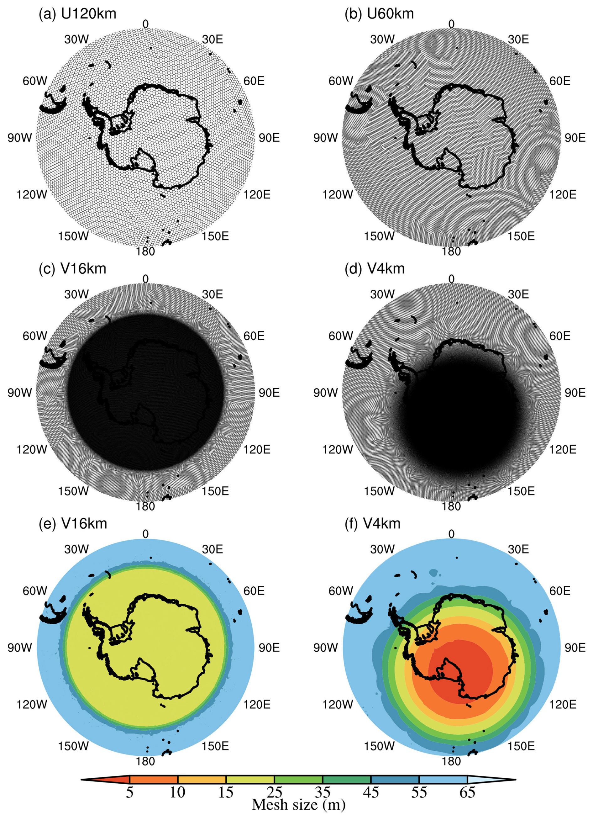
Figure 1 (a) Global quasi-uniform-resolution mesh with a grid spacing of 120 km (U120km). (b) Global quasi-uniform-resolution mesh with a grid spacing of 60 km (U60km). (c) Global variable-resolution mesh with a grid spacing ranging from 16 to 60 km (V16km), featuring a refined region over the entire Antarctic continent. (d) Global variable-resolution mesh with a grid spacing ranging from 4 to 60 km (V4km), featuring a refined region over a complex terrain of Antarctica, including the Ross Ice Shelf and the Transantarctic Mountains. (e) Spatial distribution of grid size for V16km. (f) Spatial distribution of grid size for V4km.

Table 1 Characteristics of the four meshes in the experiments.

The iAMAS model is configured with 55 vertical layers and a model top at 30 km. The initial conditions for iAMAS were derived from ERA5 reanalysis data. The first 24 h are considered the initial spin-up period; only simulations from 24 to 120 h are combined to create a continuous time series for monthly analyses. Four iAMAS experiments (U120km, U60km, V16km, and V4km) were conducted over four months (January, April, July, and October) in 2015, representing the four seasons. In Antarctica, the seasons do not exhibit the distinct characteristics found in the mid-latitudes. In this study, January and October, which fall within the Antarctic polar day, are regarded as warm months, while April and July, occurring during the polar night, are considered cold months. The main physical schemes employed in this study are detailed in Table 2, which presents the common configurations for the four iAMAS experiments configured with different grid resolutions.

(Grell and Freitas, 2014)(Thompson et al., 2008)(Tewari et al., 2016)(Nakanishi and Niino, 2006)(Iacono et al., 2008)(Iacono et al., 2008)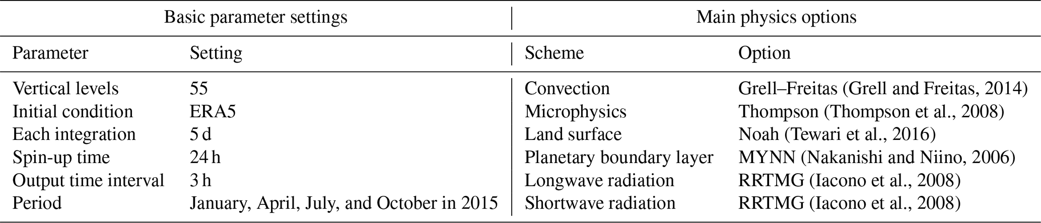

Table 2 iAMAS configurations.

2.2 Data

2.2.1 ERA5

The ERA5 dataset, employed as the initial conditions for iAMAS in this study, is the fifth-generation ECMWF reanalysis of global climate data (Hersbach et al., 2020). The motivation for using ERA5 to compare with iAMAS simulations is to analyze whether biases in iAMAS are influenced by the initialized field or arise from the model itself, which is essential for informing future model development. Additionally, the statistical results of ERA5 can serve as a reference for evaluating the statistical performance of iAMAS. ERA5 integrates model data with global observations to produce a globally complete and consistent dataset. In this study, both surface and upper-atmospheric meteorological fields from ERA5 for January, April, July, and October of 2015 are analyzed. Surface data are derived from ERA5 hourly data at single levels with a resolution of 0.25°×0.25° (https://cds.climate.copernicus.eu/cdsapp#!/dataset/reanalysis-era5-single-levels?tab=overview, last access: 7 June 2024). These surface data include 2 m temperature, surface pressure, 2 m dew point temperature (for specific humidity calculation), and 10 m wind speed. For upper-atmospheric fields, ERA5 provides data at 37 pressure levels, also with a resolution of 0.25°×0.25° (https://cds.climate.copernicus.eu/cdsapp#!/dataset/reanalysis-era5-pressure-levels?tab=overview, last access: 3 January 2024). The profile data utilized in this study include geopotential height (for altitude calculation), temperature, relative humidity (for specific humidity calculation), and wind speed.

This study analyzes specific humidity rather than relative humidity due to the high sensitivity of relative humidity calculations to temperature, particularly at typical low temperatures of Antarctica. Calculated relative humidity can exhibit significant uncertainty in Antarctica. Therefore, this study utilizes specific humidity to describe the features of Antarctic water vapor.

2.2.2 AWS

The surface-layer measurements used to evaluate iAMAS simulations were obtained from the Antarctic Meteorological Research Center (AMRC) and the AWS program in Antarctica. During the model verification period (January, April, July, and October of 2015), data from 55 AWS sites, recorded at 3 h intervals, were available on the AMRC website (ftp://amrc.ssec.wisc.edu/pub/aws/q3h/2015, last access: 9 December 2024), although some records were incomplete. These AWS locations are marked by dots in Fig. 2. The AWS measurements underwent quality control using Interactive Data Language (IDL) software (Lazzara et al., 2012). The height of the instrument for measuring meteorological parameters is nominally 3 m above the snow surface; however, this distance varies with temporal changes in the snow surface due to accumulation.

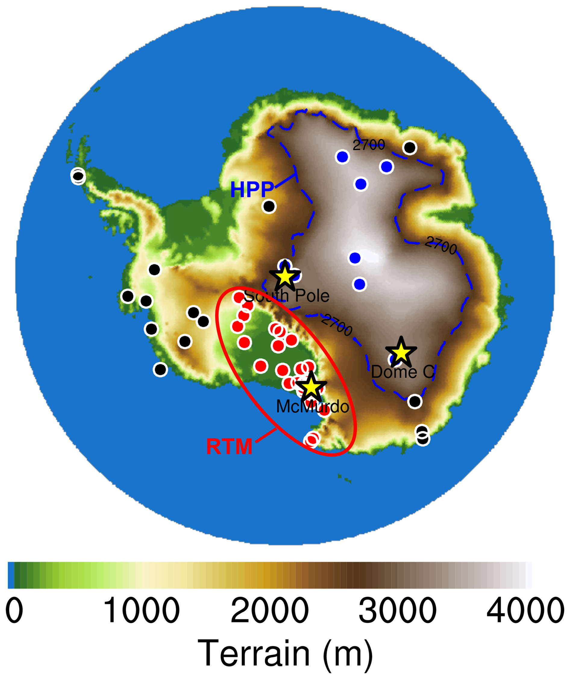
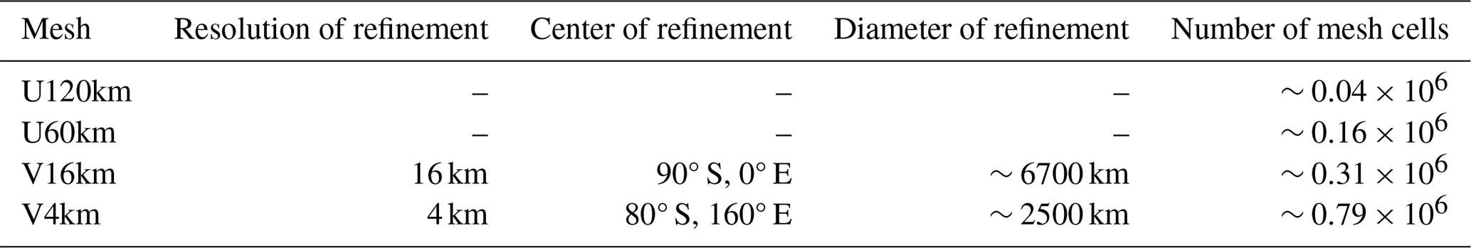
Figure 2 The elevation of the Antarctic continent and the adjacent ocean. The RTM region (including Ross Ice Shelf and Transantarctic Mountains) is delineated by a red solid line, while the HPP (High Polar Plateau) region is marked by a blue dashed line. Red and blue dots represent AWS locations within the RTM and HPP regions, respectively, whereas black dots indicate other AWS locations in Antarctica. The yellow stars with black edges denote the locations of McMurdo (78° S, 167° E), the South Pole (90° S, 0° E), and Dome C (75° S, 123° E), where sounding balloons were launched.

In this study, we define a region referred to as RTM, which includes nearly all AWS stations located on the Ross Ice Shelf and within the Transantarctic Mountains (indicated by the 29 red dots in Fig. 2). Additionally, we define a High Polar Plateau (HPP) region as areas with elevations exceeding 2.7 km, corresponding approximately to the altitude of the Henry AWS station (2755 m) near the South Pole. This region is delineated by the blue dashed line over East Antarctica, as shown in Fig. 2. The AWS stations within the HPP are marked by eight blue dots in Fig. 2. RTM is characterized by complex, low-altitude terrain and a relatively unstable atmosphere, whereas HPP is a flat region at a relatively high altitude, where strong surface temperature inversions have been observed (Yang et al., 2021a, b, 2022, 2023b). These two regions exhibit distinct features, and their meteorological fields will be analyzed in detail later.

2.2.3 Radiosonde

This study utilizes radiosonde measurements from three representative sites on the Antarctic continent: McMurdo (MM) on the coast, the South Pole (SP) on the polar plateau flank, and Dome C (DC) at the summit. MM is situated on Ross Island, near the Transantarctic Mountains, which feature relatively complex terrain within the RTM region. In contrast, SP and DC are located within the HPP region, characterized by relatively flat terrain. Daily radiosonde measurements at MM and SP are available from the AMRC (ftp://amrc.ssec.wisc.edu/pub, last access: 16 December 2024), while measurements at DC are obtained from the Antarctic Meteo-Climatological Observatory (http://www.climantartide.it, last access: 26 June 2023). The locations of these three radiosonde sites are marked by yellow stars in Fig. 2.

The radiosonde measurements provide high-resolution profiles of temperature, pressure, relative humidity (which is used to calculate specific humidity), and wind speed. Radiosonde launches at MM and the SP were generally conducted twice daily at 00:00 and 12:00 UTC during the warmer months and once daily – typically at 00:00 UTC – during the colder months. At DC, radiosondes were generally launched once daily at 12:00 UTC throughout the year. Some data are missing, likely due to the harsh Antarctic environment. In total, 182, 194, and 116 sounding profiles are available at MM, SP, and DC, respectively, for January, April, July, and October of 2015. It is important to note that MM, SP, and DC are all located within the 4 km grid resolution region of V4km in Fig. 1, allowing these radiosonde measurements to evaluate the impact of increasing iAMAS horizontal resolution to 4 km on enhancing simulations.

3 Results

3.1 Fields near the surface

The iAMAS surface-layer simulations over the Antarctic continent are evaluated by comparing them with ERA5 data and AWS measurements. The temperature, pressure, specific humidity, and wind speed within the surface layer are analyzed. Surface-layer variables from iAMAS and ERA5 are compared using the nearest points to the latitude and longitude of each AWS location. For both iAMAS and ERA5, 2 m temperature and specific humidity are used for direct comparison, despite the AWS sensors being nominally positioned 3 m above the snow surface.

Maintaining sensors at a fixed height is challenging due to snow accumulation at many sites (Lazzara et al., 2012). Blowing snow, characterized by the wind-driven transport of snow, can play an important role in snow accumulation along the escarpment regions of the Antarctic Plateau (Lenaerts and van den Broeke, 2012), where strong katabatic winds prevail. Snowfall from the sky appears to have a minor contribution, as both iAMAS and ERA5 indicate that most areas of the Antarctic continent – except for the coastal regions of West Antarctica – experience very low snowfall (see Fig. S1 in the Supplement). Moreover, the differences in snowfall between iAMAS and ERA5 across the Antarctic continent are relatively small (see Fig. S2).

Surface pressure is corrected using the hypsometric equation to account for altitude differences between the model surface (iAMAS and ERA5) and the AWS locations. For wind speed, the 10 m wind speeds from both iAMAS and ERA5 were adjusted to 3 m above the model surface using a logarithmic wind profile with a roughness length of 0.001 m to closely match the height of the AWS wind measurements.

3.1.1 2 m temperature

The seasonal variations of 2 m temperature for ERA5 are illustrated in the first column of Fig. 3. ERA5 temperature contours show that January exhibits the highest 2 m temperature compared to the other three months. The black downward triangles over the HPP region in January suggest an underestimation of 2 m temperature by ERA5. In the colder months of April and July, the upward white triangles within the HPP region indicate that ERA5 overestimates the 2 m temperature in the high interior. Temperatures in October fall within an intermediate range among the four months, with relatively small positive bias in ERA5 temperature within the HPP region during this month. In summary, the statistics across the four months suggest that ERA5 tends to underestimate high temperatures and overestimate low temperatures over the High Polar Plateau. Similarly, Gossart et al. (2019) reported that three reanalyses (ERA5, ERA-Interim, and CFSR) exhibit substantial warm biases over the Antarctic interior, particularly during winter.

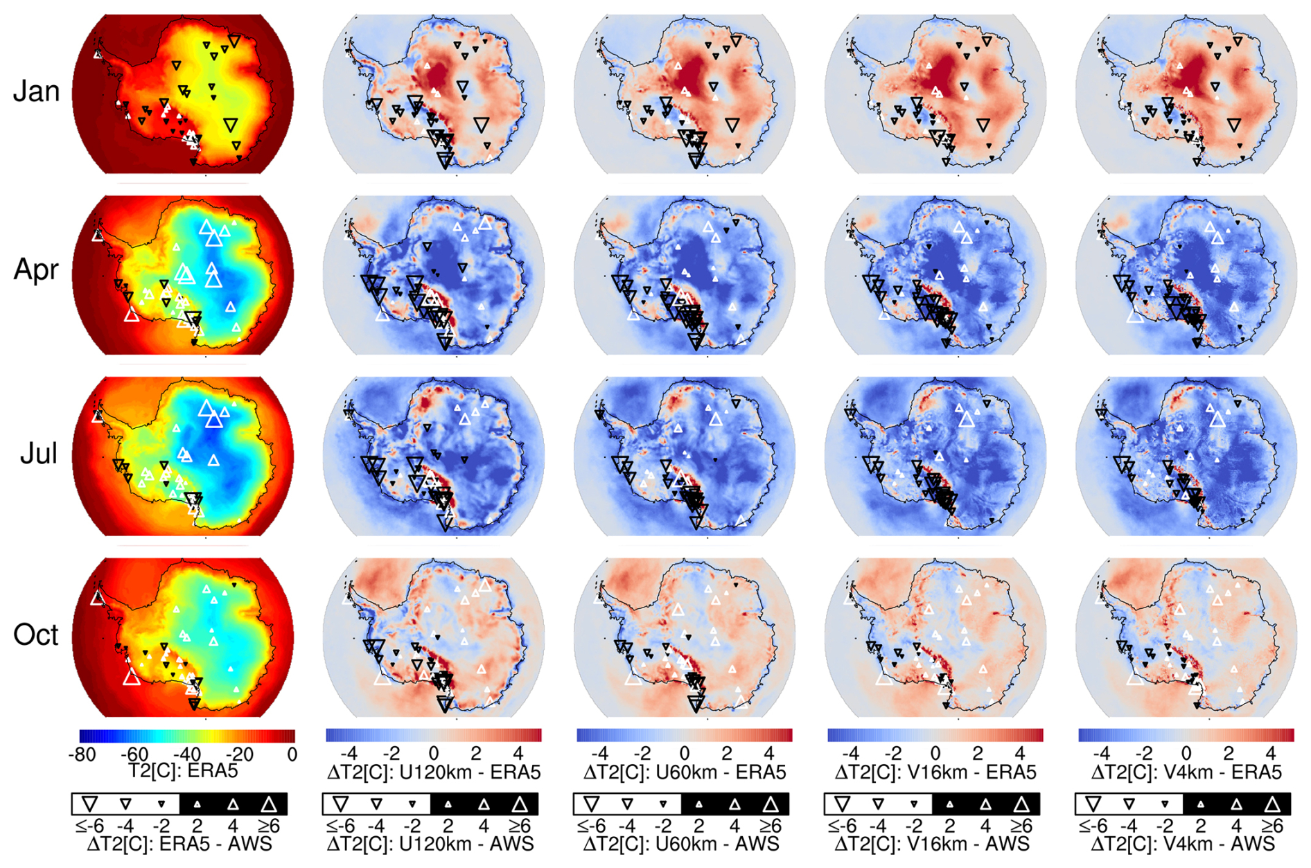
Figure 3 The first column displays the monthly median 2 m temperature (T2 [°C]) for ERA5. The four rightmost columns show the monthly median values of 2 m temperature biases (ΔT2 [°C]) for iAMAS minus ERA5. The magnitudes of the monthly median biases for the model (ERA5 or iAMAS) minus AWS are indicated by the size of the overlaid triangles: black downward-pointing triangles represent negative biases, while white upward-pointing triangles represent positive biases. Number of stations: 45 (January), 47 (April), 44 (July), and 51 (October).

The comparison of iAMAS with ERA5 in Fig. 3 reveals that all four iAMAS experiments, at various resolutions, generally simulate warmer temperatures than ERA5 in January. This warm bias may be attributed to the relatively low snow albedo value of 0.55 used in the iAMAS model. According to Xue et al. (2022), increasing the albedo to 0.8 effectively removes the strong warm bias and results in improved performance during austral summer. In April and July, iAMAS simulations exhibit colder temperatures than ERA5. In October, the simulated temperatures from iAMAS are closer to those of ERA5 than in the other three months. In particular, in April and July, the temperatures simulated by the four iAMAS experiments at various resolutions all align more closely with the AWS measurements than those from ERA5 within the HPP region. This is evidenced by the smaller sizes of the triangles indicating biases for iAMAS minus AWS compared to those for ERA5 (see April and July in Fig. 3).

Figure 4 provides an example from the South Pole over the HPP region, suggesting that ERA5 overestimates cold temperatures in April and July, while iAMAS (regardless of the chosen resolution) better captures the temperature trends during the cooling process. Fréville et al. (2014) also identified a widespread overestimation of temperature in ERA-Interim reanalysis data when compared to Moderate Resolution Imaging Spectroradiometer (MODIS) data in the Antarctic. They argue that this warm bias may result from an overestimation of surface turbulent fluxes under very stable conditions. Interestingly, we also found that the warm bias in ERA5 is associated with meteorological situations characterized by temperature inversions, as the correlation coefficient between the temperature inversion and ERA5's warm bias reaches 0.49. This confirms that ERA5 demonstrates inaccurate temperature estimations under inversion conditions in Antarctica. By comparing the turbulent heat fluxes between iAMAS and ERA5 under stable conditions for four months (January, April, July, and October) at the SP, we found that the surface turbulent sensible heat flux in iAMAS (e.g., V4km: 20.4 W m⁻²) is lower than in ERA5 (28.4 W m⁻²) during temperature inversion. These results suggest that, unlike ERA5, iAMAS may not overestimate surface turbulent heat fluxes, potentially leading to more accurate temperature predictions.

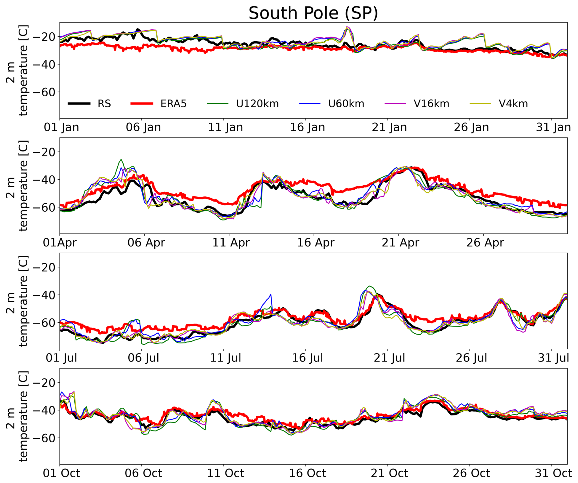
Figure 4 The time series of surface-layer temperatures at the South Pole for January, April, July, and October of 2016.

Wille et al. (2016) indicated that the Noah Land Surface Model (Noah LSM), used by iAMAS in this study, omits the sublimation process from blowing snow. Consequently, the cooling effect of sublimation may be neglected, potentially leading to an overestimation of temperature in the model during blowing snow events driven by strong winds. Interestingly, our analysis reveals that the warm bias in iAMAS slightly increases with higher wind speeds. When comparing iAMAS simulations with measurements from all AWS in Antarctica, the statistics show that a 10 m s⁻¹ increase in measured wind speed corresponds to a 0.5 K rise in the temperature difference between iAMAS and AWS.

Table 3 presents the temperature statistics from the models (ERA5 and iAMAS) in comparison to the AWS observations, including the root mean square error (RMSE) and median bias ($\text{BIAS}=\text{median}[\text{model}-\text{AWS}]$). The BIAS values for the iAMAS temperature at various resolutions over the RTM region, as shown in Table 3, are consistently negative, indicating a cold bias over the Ross Ice Shelf. This finding is consistent with the simulation results from another model (the regional atmospheric model CCLM; Zentek and Heinemann, 2020) applied to a similar environment (Filchner–Ronne Ice Shelf) in Antarctica.

Table 3 Monthly RMSE (BIAS in parentheses) of the 2 m temperature for ERA5 and iAMAS compared with AWS. The unit is °C. Number of stations within RTM: 25 (January), 26 (April), 25 (July), and 27 (October). Number of stations within HPP: 8 (January), 8 (April), 6 (July), and 8 (October).

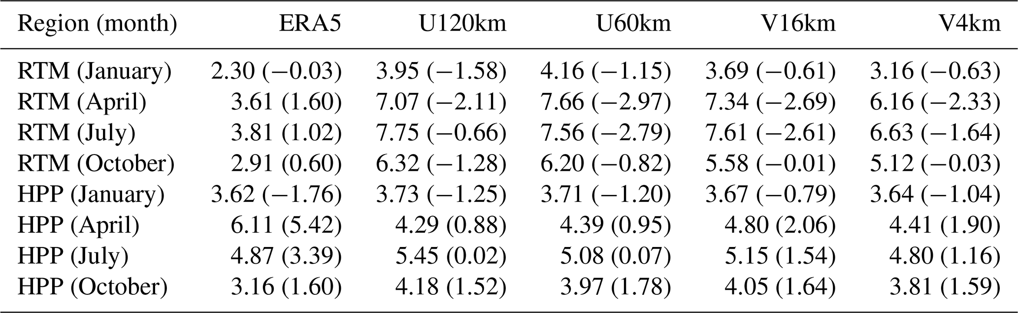
Table 3 shows that the performance of iAMAS declines during the colder months (April and July). This is consistent with the Antarctic simulation results presented by Powers and Manning (2017), who found that the temperature RMSE for WRF (MPAS) is 2.73 °C (2.14 °C) in December–January and 5.08 °C (7.24 °C) in July–August. Additionally, Xue et al. (2022) conducted Polar WRF simulations and reported that the RMSE for 2 m temperature is higher in July–August (4.03 °C) than in December–February (3.06 °C). Results from ERA5 (see Table 3 in this study) and ERA-Interim (see Xue et al., 2022) both indicate that the 2 m temperature RMSE is larger in July than in January. Thus, it can be inferred that 2 m temperature errors in the atmospheric model may be influenced, at least in part, by the lateral boundary conditions (ERA5 or ERA-Interim).

In the RTM region, both the U60km (RMSE: 4.16–7.66 °C) and V16km (RMSE: 3.69–7.61 °C) show no significant improvements and, in some cases, even perform slightly worse than the U120km (RMSE: 3.95–7.75 °C). It is the V4km (RMSE: 3.16–6.63 °C) that demonstrates improvements in temperature simulations across all four months.

In the HPP region, the magnitudes of temperature biases for iAMAS at four resolutions are all smaller than those of ERA5 during April and July (see Table 3), indicating that iAMAS more accurately captures the cooling process during these months (see the South Pole example within HPP in Fig. 4). Based on all four months' statistics presented in Table 3, U120km, U60km, V16km, and V4km demonstrate overall reductions in temperature RMSE of 0.6 %, 3.6 %, 0.5 %, and 6.6 %, respectively, compared to ERA5 in the HPP. This suggests that iAMAS performs comparably to, and in some cases better than, ERA5 in representing 2 m temperature. On the other hand, when compared to U120km, U60km shows a moderate reduction in temperature errors across this flat terrain (i.e., HPP). However, further increases in horizontal resolution from U60km to V16km (or V4km) result in minimal reductions in temperature RMSE.

In summary, a grid resolution of 4 km or finer is recommended for iAMAS to simulate 2 m temperatures in complex terrain (i.e., RTM) in Antarctica, while a resolution of 60 km seems to be adequate for flat terrain (i.e., HPP).

3.1.2 Surface pressure

The evaluation of surface pressure is presented in Fig. 5. The four rightmost columns indicate that discrepancies between iAMAS and ERA5 decrease with increasing iAMAS grid resolution. The iAMAS pressure simulations exhibit positive biases over the escarpment region and negative biases along the coast, with these biases being more pronounced for U120km compared to ERA5. This discrepancy may be due to the coarse grid of the iAMAS model that spatially smooths the topography, resulting in mismatched elevations between iAMAS and ERA5 grid points because the elevation biases (iAMAS minus ERA5) are found to be negative over the escarpment region and positive along the coast (not shown).

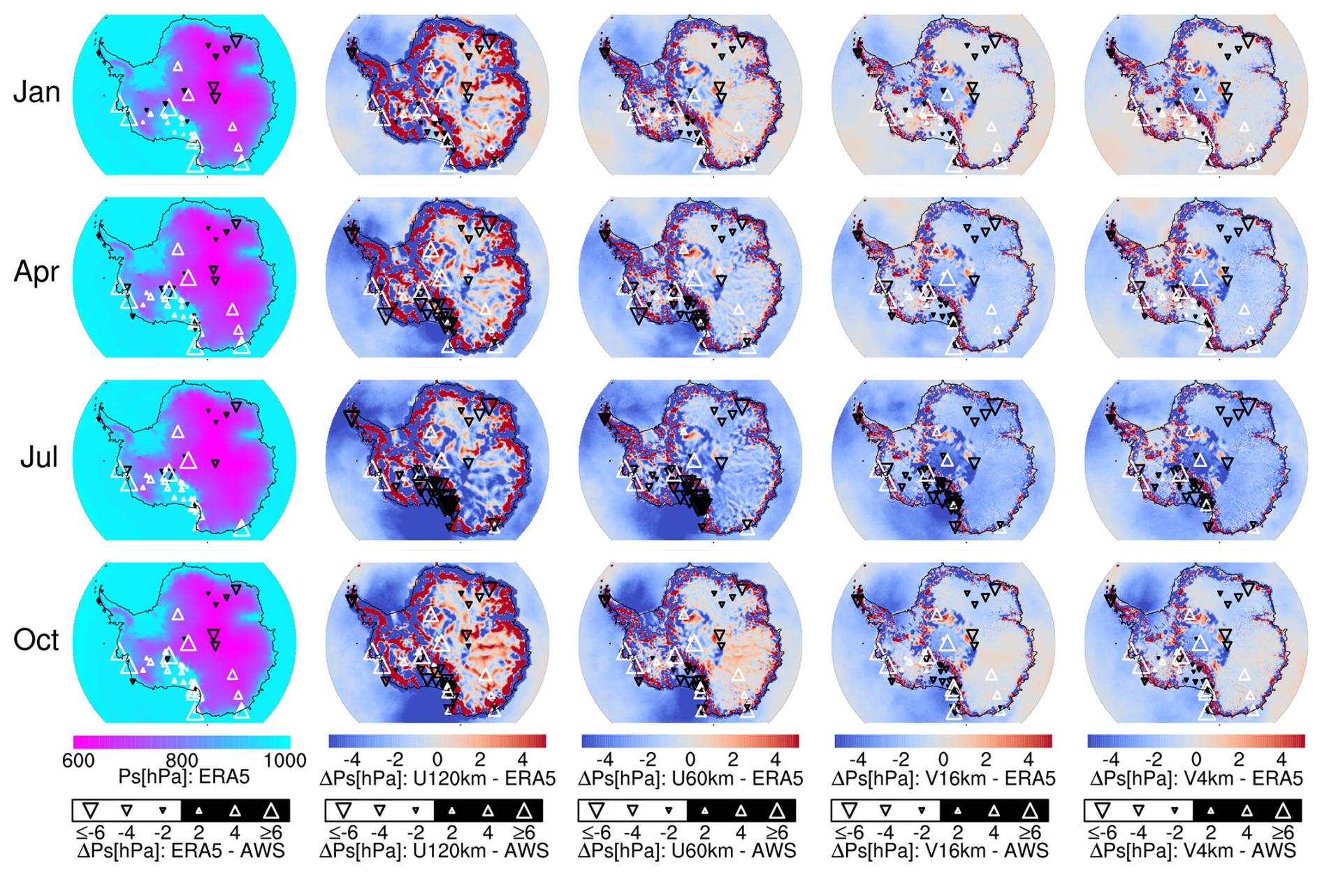
Figure 5 Same as Fig. 3 but for surface pressure (Ps [hPa]). Number of stations: 42 (January), 46 (April), 44 (July), and 48 (October).

When comparing iAMAS simulations with AWS measurements within the RTM region with complex terrain, the pressure biases for different grid resolutions all exhibit seasonal variations. Specifically, there is a smallest pressure bias in January (indicated by smaller triangles in Fig. 5) and a largest bias in July (indicated by larger triangles in Fig. 5) over the RTM region. In contrast, the HPP region does not show significant seasonal variations in pressure bias. For example, at Dome F (−77.31° S, 39.71° E) and Dome C in the HPP, the biases at Dome F remain negative (−0.32 to −1.30 hPa) across all months, while Dome C consistently exhibits positive biases (2.36–3.79 hPa). Notably, the spatial distribution of iAMAS pressure biases at four grid resolutions over HPP closely resembles that of ERA5, suggesting that the surface pressure bias in iAMAS over the flat terrain (i.e., HPP) may be attributed to its initial condition (which here is ERA5).

Table 4 presents the performance of iAMAS in simulating surface pressure. The RMSE and BIAS presented in Table 4 were calculated using adjusted pressure, applying the hypsometric relationship to reduce biases arising from height differences between the surface grids of the models (iAMAS and ERA5) and the AWS sensors. This adjustment strategy has effectively reduced the pressure bias. For instance, the pressure RMSE of U120km within the RTM region in January is 20.48 hPa without using the hypsometric relationship, whereas the RMSE for the adjusted pressure is only 2.41 hPa.

Table 4 Monthly RMSE (BIAS in parentheses) of the surface pressure for ERA5 and iAMAS compared with AWS. The unit is hPa. Number of stations within RTM: 22 (January), 24 (April), 24 (July), and 24 (October). Number of stations within HPP: 8 (January), 8 (April), 6 (July), and 8 (October).

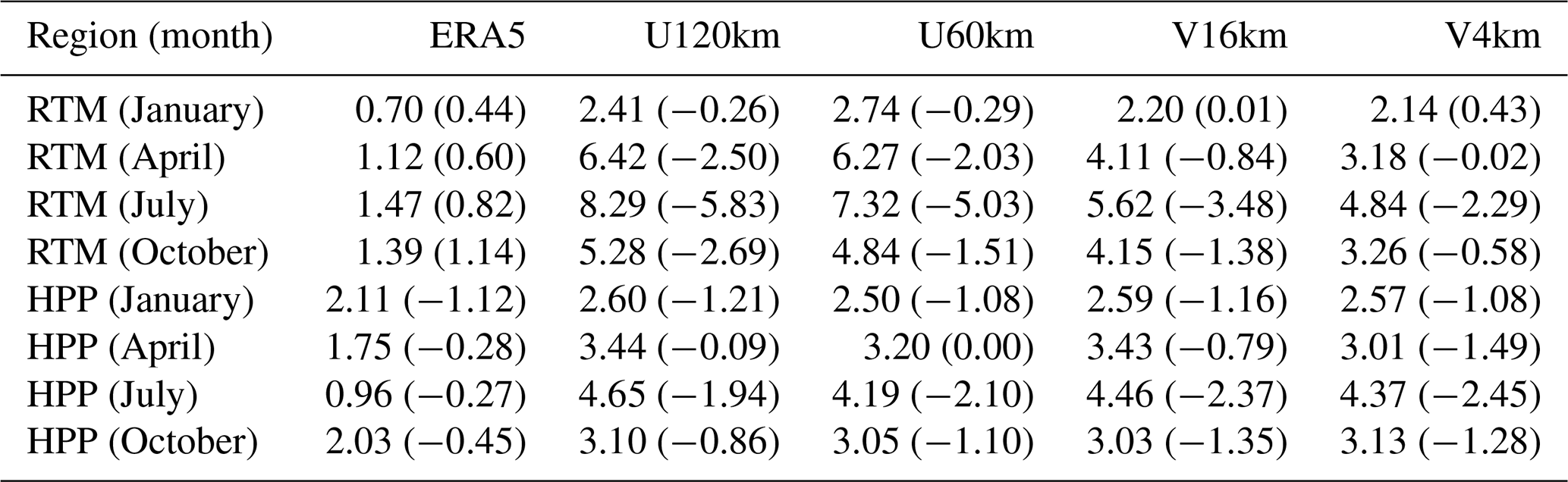
Table 4 demonstrates that the surface pressure of ERA5 is closer to the AWS observations, showing smaller RMSE values than iAMAS. This is expected because ERA5 is an analysis product that assimilates AWS observations. In contrast, iAMAS operates as a forecast model: it starts from initial conditions (i.e., ERA5) at the first time step and, as a global model, does not require boundary conditions during the run. Consequently, its forecasts may drift away from the initial conditions over time.

In the RTM region, a finer resolution is essential, as the pressure RMSE decreases from U120km (RMSE: 8.29–2.41 hPa) to V4km (RMSE: 4.84–2.14 hPa). In contrast, for the HPP, Table 4 indicates that a 60 km grid resolution is sufficient for iAMAS to simulate pressure, as further increases in grid resolution yield minimal improvements.

3.1.3 2 m specific humidity

Figure 6 illustrates the biases in 2 m specific humidity. In the HPP region, ERA5 predominantly exhibits wet biases throughout the year. In contrast, all four iAMAS experiments at various resolutions show clear seasonal variations over the HPP region. Dry biases are more pronounced during the warmer months of January and October, while wet biases become more prominent during the colder months of April and July. It is worth noting that measuring atmospheric moisture content at low air temperatures is challenging due to the extremely small amounts of water vapor present. Lazzara et al. (2012) also noted that humidity measurement errors tend to increase under low-temperature conditions.

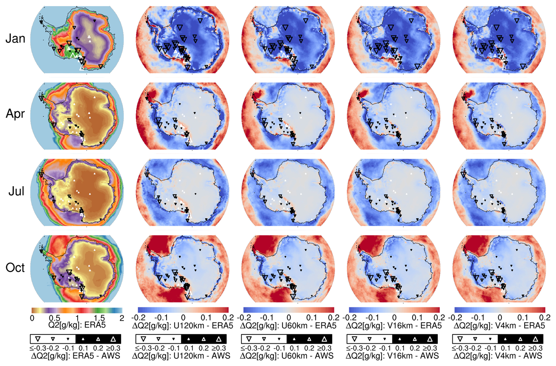
Figure 6 Same as Fig. 3 but for 2 m specific humidity (Q2 [g kg⁻¹]). Number of stations: 32 (January), 34 (April), 35 (July), and 35 (October).

Table 5 presents the RMSE and BIAS for 2 m specific humidity. In the RTM region, iAMAS specific humidity values at various resolutions are consistently drier than those from AWS, e.g., BIAS values for U120km ranging from −0.0009 to −0.2404 g kg⁻¹. Similar dry biases were also noted in AMPS simulations (Wille et al., 2016), which suggested that this underestimation may arise from the Noah LSM, which is also used by iAMAS in this study. The Noah LSM does not account for sublimation from drifting and blowing snow near the surface. Furthermore, the magnitudes of underestimation in iAMAS simulations at various resolutions are all greater during the warm months than in the cold months within the RTM region. Notably, increasing the grid resolution from U120km (RMSE: 0.1853–0.5786 g kg⁻¹) to V4km (RMSE: 0.1613–0.4601 g kg⁻¹) can reduce humidity errors over the RTM region. In the HPP region, increasing the iAMAS grid resolution does not significantly improve specific humidity simulations.

Table 5 Monthly RMSE (BIAS in parentheses) of the 2 m specific humidity for ERA5 and iAMAS compared with AWS. The unit is g kg⁻¹. Number of stations within RTM: 20 (January), 21 (April), 21 (July), and 20 (October). Number of stations within HPP: 5 (January), 5 (April), 4 (July), and 5 (October).

Spatially, the RTM region, characterized by lower altitudes, experiences warmer air compared to the HPP. The iAMAS simulations exhibit more pronounced dry biases in the RTM than in the HPP. Temporally, dry biases are more significant during the warm months than in the cold months. In summary, iAMAS appears to underestimate specific humidity in warmer conditions.

3.1.4 3 m wind speed

Persistent katabatic winds are a distinctive meteorological phenomenon over the Antarctic plateau. This is evident from the ERA5 3 m wind speed data shown in the first column of Fig. 7, which illustrates an increase in wind speed from the summit of the inland plateau to the escarpment region, where katabatic winds prevail over the escarpment region with steep surface (Parish and Cassano, 2001; Ma et al., 2010; Rinke et al., 2012). Figure 7 indicates that iAMAS at various resolutions always reproduces stronger wind speeds than ERA5 over complex terrain, particularly just inland from the coast and the Transantarctic Mountains. The iAMAS simulations with higher grid resolutions show a reduction in such positive wind bias. As grid resolution increases, iAMAS better resolves the complex terrain, enhancing the blocking/barrier effect of rough underlying terrain on the near-surface wind field flow (similar to Argentini and Mastrantonio, 1994; O'Connor and Bromwich, 1988), which subsequently leads to decreased wind speeds in the iAMAS simulations. Similarly, Bromwich et al. (2005) compared the AMPS 10 and 3.3 km resolution MM simulation domains and found that the higher-resolution (3.3 km) domain provides a more accurate depiction of near-surface winds; they argued that the positive bias in wind speed is partly due to topographic smoothing.

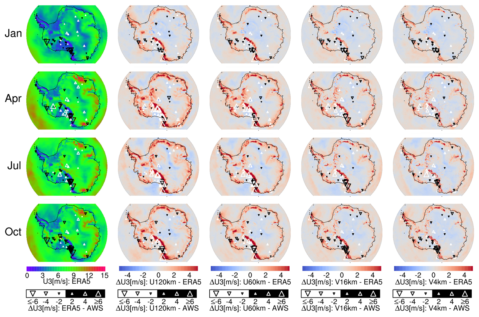
Figure 7 Same as Fig. 3 but for 3 m wind speed (U3 [m s⁻¹]). Number of stations: 41 (January), 42 (April), 41 (July), and 47 (October).

Table 6 shows that the wind speed performance of iAMAS declines during the colder months (April and July). Powers and Manning (2017) also observed that wind speed simulations exhibit a similar performance decline in Antarctic winter, with the near-surface wind speed RMSE in East Antarctica for WRF (MPAS) being 1.45 m s⁻¹ (1.41 m s⁻¹) for December–January and 2.49 m s⁻¹ (1.93 m s⁻¹) for July–August. In addition, Xue et al. (2022) conducted Polar WRF simulations and reported that the RMSE for 10 m wind speed is higher in July–August (4.20 m s⁻¹) than in December–February (3.20 m s⁻¹). Reanalysis data are typically used as lateral boundary conditions for atmospheric models. Four reanalyses (ERA5, ERA-Interim, CFSR, and MERRA-2) consistently show degraded performance in reconstructing near-surface wind speeds during the Antarctic winter compared to summer (see Table 6 in this study; Xue et al., 2022; Gossart et al., 2019). These findings suggest that errors in near-surface wind speed simulations using both iAMAS and WRF may be partially attributed to deficiencies in their reanalysis-based boundary conditions.

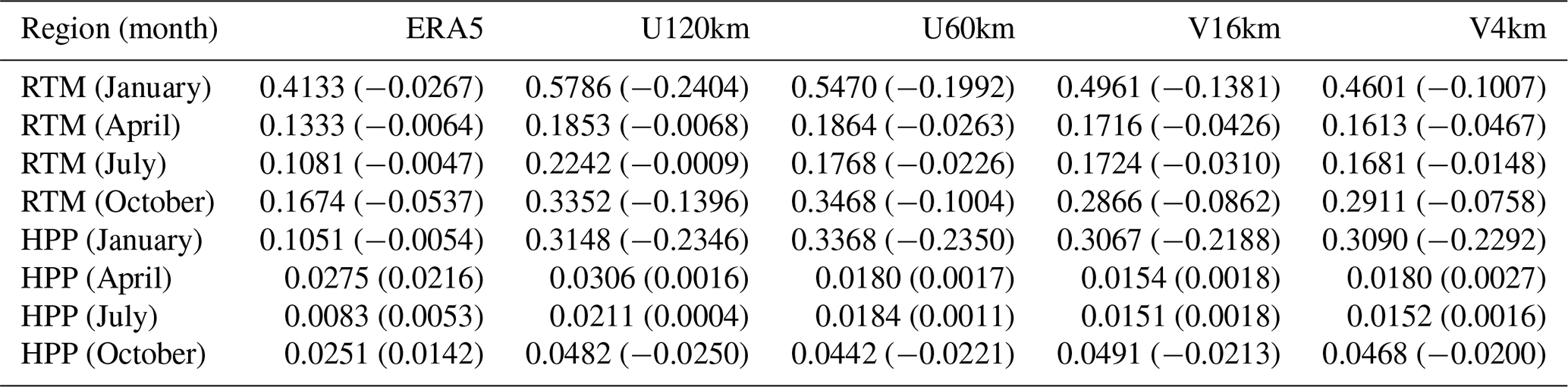
Table 6 Monthly RMSE (BIAS in parentheses) of the 3 m wind speed for ERA5 and iAMAS compared with AWS. The unit is m s⁻¹. Number of stations within RTM: 23 (January), 24 (April), 24 (July), and 26 (October). Number of stations within HPP: 8 (January), 8 (April), 6 (July), and 8 (October).

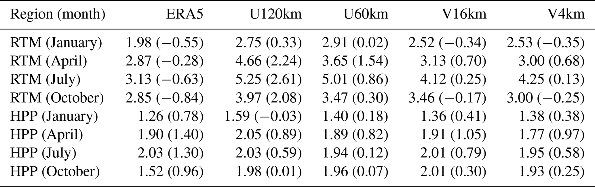
In the context of complex terrain (i.e., RTM), Table 6 demonstrates that increasing the iAMAS grid resolution enhances wind speed simulations. The RMSE for wind speed has decreased from U120km (RMSE: 2.75–5.25 m s⁻¹) to V4km (RMSE: 2.53–4.25 m s⁻¹). Notably, U120km tends to overestimate wind speeds (BIAS: 0.33–2.61 m s⁻¹), whereas the high-resolution iAMAS simulations (e.g., V4km with a BIAS of −0.35 to 0.68 m s⁻¹) indicate a smaller wind speed positive bias. As previously discussed, the barrier effect of mountains becomes more pronounced with a higher-resolution grid, leading to a decrease in wind speed.

Over the HPP region with flat terrain, Table 6 shows that the performance of iAMAS in simulating wind speed is comparable to that of ERA5. For example, the RMSE for U120km (RMSE: 1.59–2.05 m s⁻¹) is quite close to that of ERA5 (RMSE: 1.26–2.03 m s⁻¹). In such flat regions, there is little difference in the RMSE statistics between the four iAMAS experiments with different grid resolutions. Once again, the results suggest that increasing model grid resolution over flat regions in Antarctica is not critically necessary.

3.2 Upper atmospheric fields

The iAMAS simulations were evaluated against radiosonde measurements from three sites (MM, SP, and DC) to assess their performance in the upper atmosphere over the Antarctic continent. To ensure robust results, data corresponding to altitudes reached by radiosondes fewer than 5 times per month were excluded. ERA5 data, used as the initial conditions for iAMAS, were also utilized for site analyses of upper-air meteorological fields. Observations and simulations from four months (January, April, July, and October 2015), consistent with the surface-layer analyses (Sect. 3.1), were collected.

The extracted model results (iAMAS and ERA5) for comparison were derived from the nearest grid points to the balloon launch sites. Balloons drifted significantly (by tens of kilometers) due to stronger winds in the stratosphere, which may increase the distance between the model grid point and the balloon, causing potential meteorological deviations. However, the stratosphere is generally stable, and we found that the meteorological fields within this layer from iAMAS varied slightly between the balloon launch and explosion locations (not shown). In contrast, the troposphere, especially near the ground, is relatively unstable, leading to substantial spatial variability in meteorological fields. Thus, using the nearest model grid to the ground-launching position may be more appropriate for analyzing the model's performance. Additionally, time differences greater than 2 hours between model data (ERA5 and iAMAS) and radiosonde measurements were excluded from the comparison. Finally, both radiosonde measurements and ERA5 reanalysis data were linearly interpolated to the height of the iAMAS grid for each site.

3.2.1 Upper-air temperature

The monthly median differences in temperature profiles between the models (ERA5 and iAMAS) and radiosonde measurements above ground level (AGL) are illustrated in Fig. 8. The absence of values in the upper atmosphere for July suggests that the radiosonde balloons do not ascend as high as in other months, likely due to the fragility of the balloon's elastic material in colder seasons, which makes them more prone to explosion (Hagelin et al., 2008).

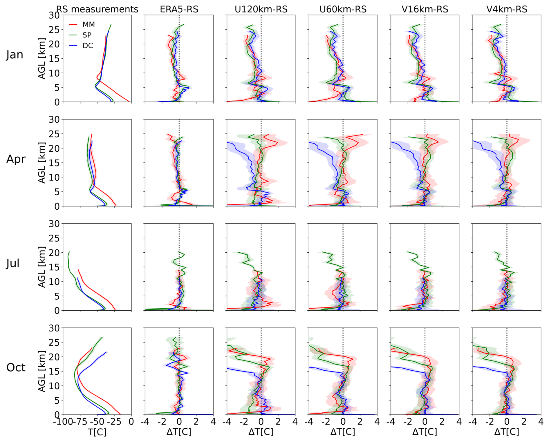
Figure 8 The first column displays the monthly medians of radiosonde-measured temperature (T [°C]) profiles. The five rightmost columns present the monthly median temperature biases (ΔT [°C]) for ERA5 and iAMAS (U120km, U60km, V16km, and V4km) compared to radiosonde measurements. The shading represents the standard error.

Near the ground at MM, both U120km and U60km exhibit a clear tendency to increase negative biases very close to the surface, potentially resulting in more pronounced surface temperature inversions. Here, we defined the inversion intensity as the temperature gradient between the second grid (76.6 m) and the first grid (23.5 m) a.g.l. The results for April indicate that U120km (22.1 K km⁻¹) exhibits stronger temperature inversions compared to the radiosonde measurements (2.9 K km⁻¹). This model error, characterized by overestimated temperature inversions, was also observed in the AMPS simulations (Silber et al., 2019), which attributes this error to the model's underestimation of surface downwelling longwave radiation. Encouragingly, a comparison of the rightmost four columns in Fig. 8 shows that increasing grid resolution can reduce the bias in the iAMAS simulated near-ground temperature at MM.

Significant temperature deviations have been observed at high altitudes in the iAMAS simulations, particularly in October, with a cold bias exceeding 10 °C at 20 $\mathrm{km}\mathrm{a}.\mathrm{g}.\mathrm{l}.$ (see Fig. 8). The temperature deviations between ERA5 and radiosonde observations are smaller than those of iAMAS. It is important to note that ERA5 is an analysis product that assimilates radiosonde observations, whereas iAMAS operates as a forecast model whose forecasts may drift away from its initial conditions (i.e., ERA5).

These high-altitude temperature deviations have been identified across different grid resolutions. Additionally, significant cold biases at such altitudes during this period have also been reported in AMPS simulations (Yang et al., 2023a). The model lids for both iAMAS and AMPS are set at approximately 10 hPa, classifying them as low-top models. In contrast, high-top atmospheric models, with a model top at or above 1 hPa, have been shown to produce more accurate simulations of winds and temperatures, as demonstrated by global atmospheric modeling evaluations (Lawrence et al., 2022; Zhao et al., 2016). Regarding polar simulation studies, the Whole Atmosphere Community Climate Model – a high-top model – exhibits improvements over the low-top version of the Community Atmosphere Model (CAM; Gettelman et al., 2019). In addition, for the Southern Hemisphere polar vortex final warming date, ensembles of high-top models from the fifth Coupled Model Intercomparison Project (CMIP5) show better agreement with reanalysis data than low-top ensembles (Wilcox and Charlton-Perez, 2013). Thus, employing a high-top model may enhance the accuracy of stratospheric simulations in Antarctica. In addition, the cold biases observed above approximately 15 km may also be attributed to the fact that the iAMAS model used in this study does not explicitly consider stratospheric ozone concentrations and their effects on radiation.

Figure 8 shows that the higher temperature biases are pronounced at both the lower and upper atmospheric levels. Xue et al. (2022) reported similar findings; for example, in July, they found that the temperature bias (Polar WRF–Observation) is −0.85 °C at 975 hPa and 0.11 °C at 100 hPa, while it is only 0.04 °C at 600 hPa. Their results indicate that temperature variability is greater near the surface and upper levels, with a broader temperature spread observed in these regions.

Figure 8 illustrates that discrepancies between iAMAS simulations with different grid resolutions primarily occur in the lower troposphere. Then, the temperature RMSE and BIAS for the 0–5 km altitude range are presented in Table 7. Additionally, temperature (as well as pressure, specific humidity, and wind speed; to be discussed later) statistics for the 5–15 and 15–25 km ranges are included in Table S1–S8 in the Supplement for readers interested in high-altitude simulation performance. The statistics for the 5–15 and 15–25 km ranges indicates that the iAMAS simulation performance is similar for different-resolution meshes. The BIAS values in Table 7 for all iAMAS simulations with various resolutions at the MM site are negative, indicating a cold bias for each month in this coastal region, consistent with the surface-layer statistics (see RTM in Table 3). V4km (RMSE: 1.55–3.41 °C) demonstrates a superior representation of temperature at the MM site compared to U120km (RMSE: 3.29–5.72 °C), highlighting the importance of increasing grid resolution in coastal areas.

Table 7 Monthly RMSE (BIAS in parentheses) of the 0–5 km temperature (°C) for ERA5 and iAMAS compared with radiosondes.

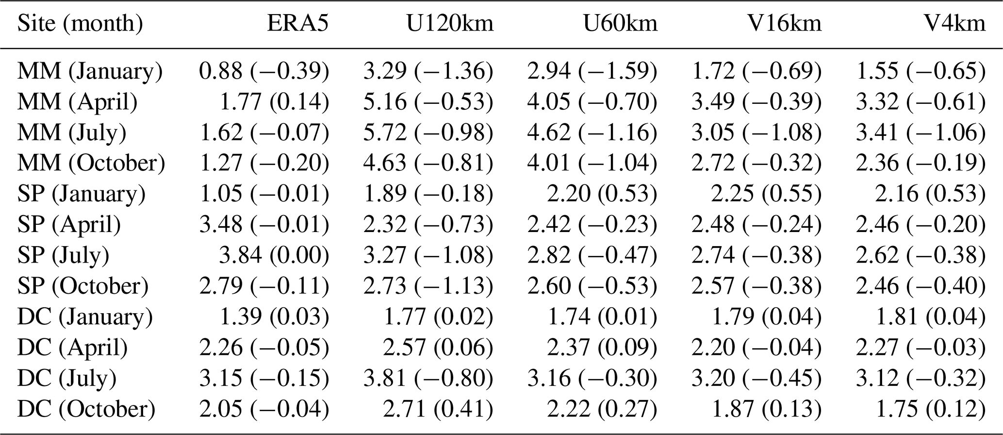
In the relatively flat region of central East Antarctica, which includes SP and DC, the representation of temperature at 0–5 km does not improve with higher-resolution iAMAS simulations across all months. For instance, in January, U60km (RMSE: 2.20 °C) performs slightly worse than U120km (RMSE: 1.89 °C) at SP, while in July, the temperature RMSE at SP moderately decreases from U120km (RMSE: 3.27 °C) to U60km (RMSE: 2.82 °C). Overall, there is little difference in the simulation results across the various iAMAS resolutions in these flat regions. It is noteworthy that during the colder months (April and October), the performance of iAMAS simulations can be comparable to, and occasionally better than, ERA5 at SP and DC. For example, in April, the temperature RMSE for U120km is 2.32 °C at SP, which is lower than that of ERA5 (RMSE: 3.48 °C).

Overall, the temperature profile statistics exhibit a performance similar to those of the surface-layer evaluation (Sect. 3.1.1), indicating that high-resolution grids for iAMAS should be employed in complex terrain. On the other hand, the V4km configuration incorporates regional mesh refinement over RTM, as opposed to the broader refinement applied across the entire Antarctic continent in the V16km configuration. Notably, V4km (last column in Table 7) performs better than V16km (second-to-last column in Table 7), suggesting that variable-resolution refinement should specifically focus on complex terrain to optimize computational efficiency.

3.2.2 Upper-air pressure

Figure 9 illustrates the statistical analysis of pressure biases. ERA5 displays a positive pressure deviation at all three sites, with a particularly notable deviation at the DC site.

Figure 9 Same as Fig. 8 but for the pressure (P [hPa]) profile.

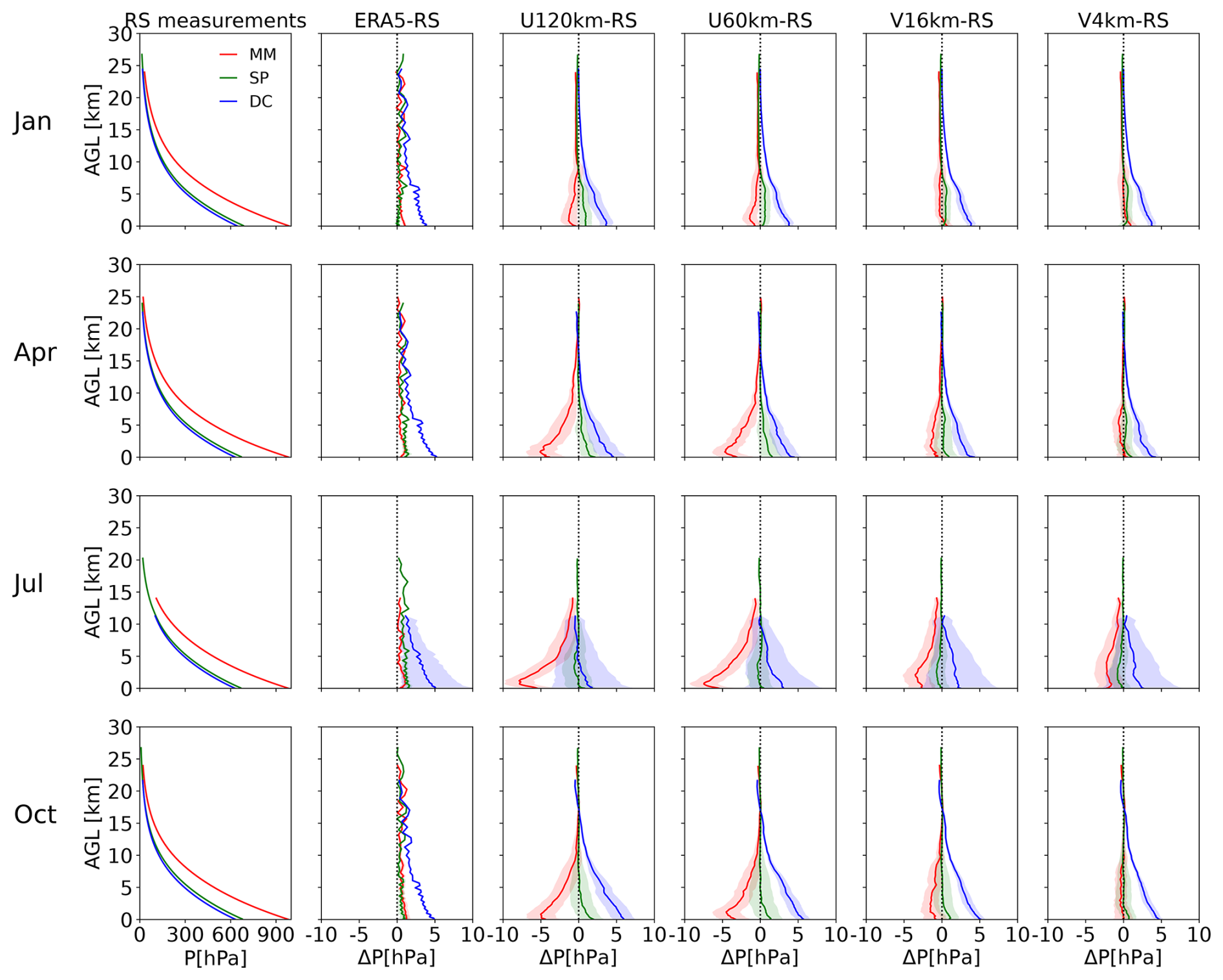
The discrepancies between all iAMAS simulations at various resolutions and radiosonde measurements exhibit minimal seasonal variation; the pressure biases at MM are consistently negative across all months, while the biases at DC are predominantly positive. The pressure bias at MM has significantly decreased from U120km to V4km (refer to the four rightmost columns of Fig. 9). This improvement is likely because high-resolution iAMAS can resolve terrain height more accurately, thus providing a better representation of pressure, as atmospheric pressure is strongly related to altitude. We observed that the actual altitude for launching the balloon at MM is 10 m. The model surface elevation of V4km (2 m) is considerably closer to the terrain height of MM compared to U120km (110 m; significant overestimation); thus, V4km yields a more accurate pressure profile.

To align with the height range of temperature statistics (Sect. 3.2.1), pressure errors within the 0–5 km altitude range have also been calculated, as detailed in Table 8. The pressure RMSE over complex terrain (i.e., MM) exhibits a substantial reduction from U120km (RMSE: 7.78–2.30 hPa) to V4km (RMSE: 4.15–1.45 hPa). As noted previously, U120km significantly overestimates the terrain height at MM; atmospheric pressure typically decreases with increasing altitude, which accounts for the negative pressure bias in U120km simulations at MM (BIAS: −0.97 to −5.90 hPa) shown in Table 8. In contrast, for SP and DC over flat regions, the increase in grid resolution for iAMAS does not result in a significant decrease in pressure RMSE as observed at the MM site. This is because the accuracy of terrain height over the flat region can be satisfactorily resolved by iAMAS even with a coarse mesh.

Table 8 Monthly RMSE (BIAS in parentheses) of the 0–5 km pressure (hPa) for ERA5 and iAMAS compared with radiosondes.

The performances of geopotential height simulations are presented in Fig. S3 and Table S9. Figure S3 shows that ERA5 exhibits overall positive geopotential height deviation at all three sites, with a particularly pronounced deviation at the DC site. At MM, the geopotential height biases are consistently negative across all months except near the model top, while those at DC are predominantly positive. Table S9 presents a statistical evaluation of the 500 hPa geopotential height, indicating that iAMAS performs better in simulating geopotential height during warmer months (e.g., January) than in colder months (e.g., July), which is consistent with the results of Polar WRF simulations over Antarctica reported by Xue et al. (2022).

3.2.3 Upper-air specific humidity

Figure 10 demonstrates that the specific humidity bias curve for all iAMAS experiments at various resolutions closely resembles that of ERA5. Therefore, the specific humidity bias in the upper air for iAMAS may be partly attributed to its initial conditions generated by ERA5. Comparisons of iAMAS simulations across different grid resolutions (see the four rightmost columns in Fig. 10) indicate that the specific humidity bias profile at MM is more significantly influenced by grid resolution, while the shape of the bias profile at SP and DC shows minimal sensitivity to horizontal resolution. It seems that grid resolution has a negligible impact on specific humidity over the flat regions represented by SP and DC, which is similar to surface-layer specific humidity analyses (Sect. 3.1.3). In October, Fig. 10 shows the underestimation of specific humidity in the stratosphere, which may be due to the cold bias (see Fig. 8) in the stratosphere and corresponds to the underestimation of atmospheric water vapor capacity.

Figure 10 Same as Fig. 8 but for the specific humidity (Q [g kg⁻¹]) profile.

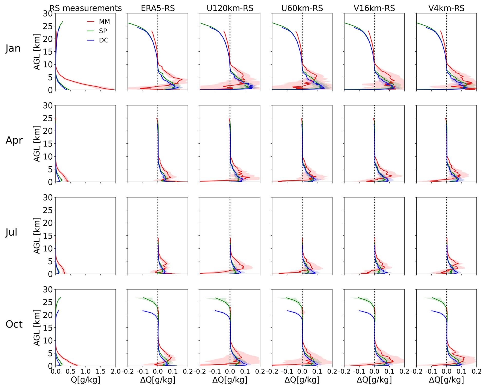
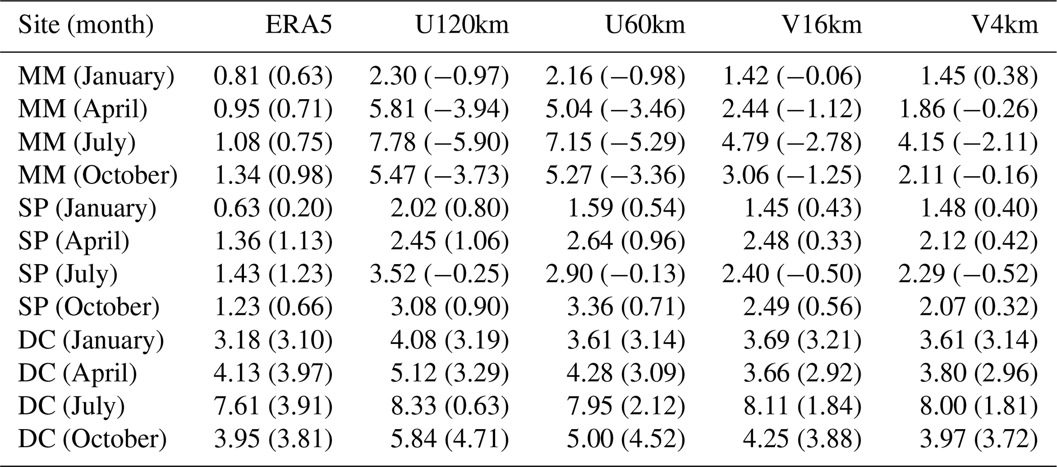
Table 9 summarizes the statistics on RMSE and BIAS derived from specific humidity measurements within the 0–5 km altitude range. ERA5 generally overestimates the specific humidity, with BIAS values at the three sites varying from 0.0212 to 0.0839 g kg⁻¹. All four iAMAS experiments at various resolutions overestimate the specific humidity. The comparison of iAMAS simulations at different resolutions presented in Table 9 reveals that specific humidity simulations at MM, which features complex terrain, improve with finer iAMAS grid resolution, as RMSE decreases from U120km (RMSE: 0.1784–0.4625 g kg⁻¹) to V4km (RMSE: 0.1215–0.3558 g kg⁻¹). However, in flat regions (i.e., SP and DC), specific humidity RMSE shows a negligible reduction with finer iAMAS grid resolution.

Table 9 Monthly RMSE (BIAS in parentheses) of the 0–5 km specific humidity (g kg⁻¹) for ERA5 and iAMAS compared with radiosondes.

Snow formation is closely related to humidity. Comparing ERA5 snowfall with iAMAS simulations shows that increasing the iAMAS grid resolution reduces snowfall overestimations over the complex terrain of West Antarctica (see Fig. S2).

In summary, high-resolution grids enhance simulation accuracy for specific humidity profiles in complex terrain but are not significant in flat terrain.

3.2.4 Upper-air wind speed

ERA5 data for wind speed exhibit polar singularity issues. According to the ERA5 Climate Data Store (CDS: https://confluence.ecmwf.int/pages/viewpage.action?pageId=129134800, last access: 30 April 2025), at the poles (i.e., at 90° N and 90° S), the U and V components of the wind are significantly underestimated. This problem arose from the way winds were derived from vorticity and divergence in the spherical harmonics representation (the native model format) when interpolated onto a regular latitude-longitude grid in the CDS. Currently, it is not anticipated that this issue will be resolved. As recommended by the ERA5 CDS, data from grid points at a latitude of 89.75° S are used to represent the wind speed at the SP to avoid the polar singularity issues.

Concerning the 3 m wind speed (Sect. 3.1.4), the ERA5 data at the SP do not exhibit significant underestimation when compared to the AWS measurements. This is because the two AWS sites (HEN: 89.02° S, 1.03° W; NIC: 89.00° S, 89.67° W) at the South Pole are not located exactly at the polar grid center (90° S), thereby avoiding the polar singularity problem.

The biases for the wind speed profile are displayed in Fig. 11. The wind speed bias for ERA5 is generally below 1 m s⁻¹ across a large portion of the atmosphere (see the second column in Fig. 11). The wind speed simulated by all four iAMAS experiments with various resolutions at the SP seems unaffected by the ERA5 initialized field at 90° S and yields overall reasonable results. This may be attributed to the limited influence of a single grid point (i.e., the point at 90° S, 0° E) on the iAMAS simulations.

Figure 11 Same as Fig. 8 but for the wind speed (U [m s⁻¹]) profile.

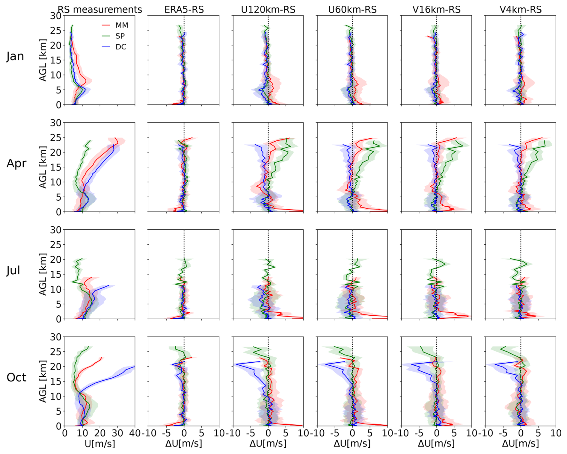
In October, Fig. 11 shows an underestimation of wind speed in the stratosphere, which corresponds to the underestimation of temperature in the same region (see Fig. 8). This suggests that iAMAS may overestimate the extent of the low-temperature region surrounding the Antarctic vortex, leading to a simulated northerly shift of the strong wind belt associated with the vortex. As a result, lower wind speeds are simulated at MM.

Near the surface, iAMAS (specifically with coarse grid resolution, e.g., U120km) tends to simulate stronger wind speeds at MM. MM is located within the RTM region; this positive bias in wind speed over such complex terrain is consistent with the surface-layer analyses (Sect. 3.1.4). In the stratosphere, larger wind speed deviations have been observed in the iAMAS simulations across different grid resolutions, particularly in April, July, and October. The high-altitude wind speed biases may also be partly attributed to the limitations of the low-top version of the iAMAS model used in this study. This study primarily focuses on tropospheric simulations, which appear to be more sensitive to model grid resolution, while research on high-altitude stratospheric simulations is currently ongoing.

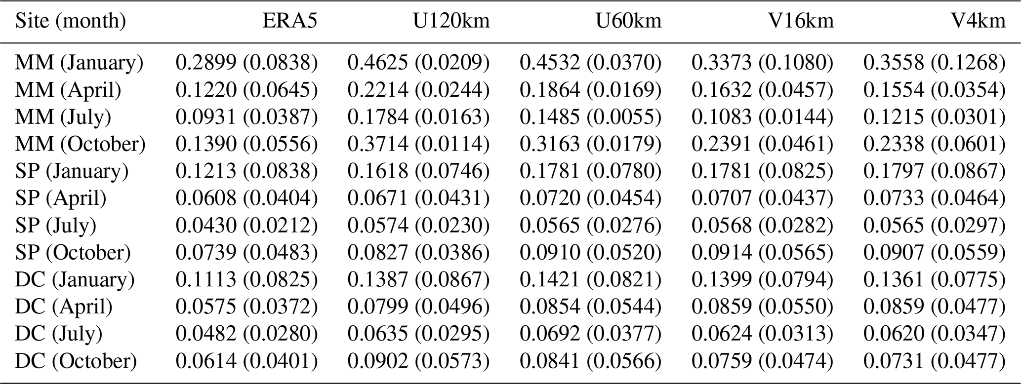
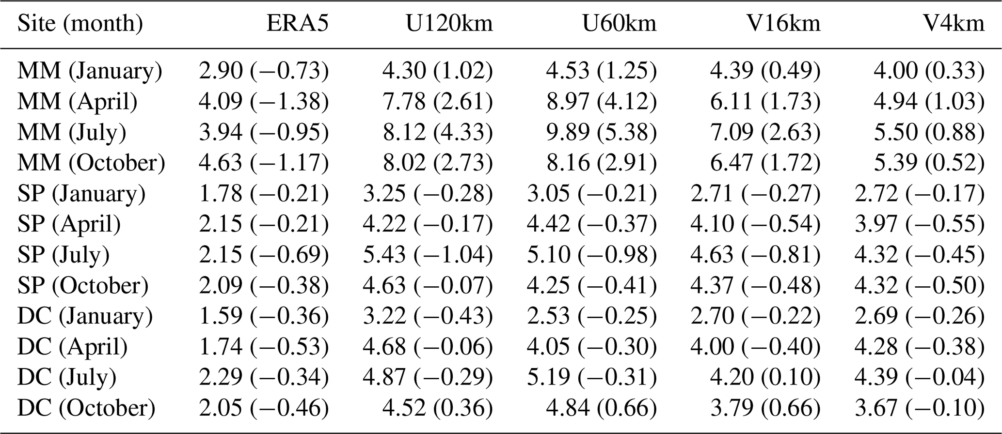
Table 10 demonstrates that the RMSE of wind speed in the 0–5 km range at MM is decreased from U120km (RMSE: 4.30–8.12 m s⁻¹) to V4km (RMSE: 4.00–5.39 m s⁻¹). This improvement can be attributed primarily to the more representative topography of the 4 km domain, as further evidenced by the comparison of 3 m wind speed simulations with AWS measurements over RTM (Sect. 3.1.4). For DC and SP in the flat HPP region, Table 10 indicates that the RMSE of the wind speed simulations shows only minor variations across different iAMAS grid resolutions. For instance, at the SP, U60km (RMSE: 3.05–5.10 m s⁻¹) exhibits slight improvements over U120km (RMSE: 3.25–5.43 m s⁻¹), whereas employing the computationally intensive V4km (RMSE: 2.72–4.32 m s⁻¹) does not significantly decrease the wind speed RMSE.

Table 10 Monthly RMSE (BIAS in parentheses) of the 0–5 km wind speed (m s⁻¹) for ERA5 and iAMAS compared with radiosondes.

4 Conclusions and discussions

Measurements from AWS and radiosondes collected on the Antarctic continent have been employed to assess the performance of an atmospheric model utilizing an unstructured SCVT mesh. The atmospheric model used in this study is the iAMAS model, which is equipped with various global mesh configurations (U120km, U60km, V16km, and V4km). Additionally, ERA5 data, serving as initial conditions for the iAMAS model, are included for comparative purposes. This study evaluates the performance of the iAMAS model concerning four routine meteorological fields, i.e., temperature, pressure, specific humidity, and wind speed, from both the surface layer and the upper air. This study serves as a valuable reference for implementing Antarctic simulations using a global model with an unstructured SCVT mesh.

A series of iAMAS simulations with lead times ranging from 2 to 5 d were combined to create a continuous time series for January, April, July, and October of 2015, allowing for an investigation of the seasonal characteristics of simulation bias. Two distinct regions, i.e., HPP with flat terrain and RTM with complex terrain, were emphatically analyzed. Performance statistics, including RMSE and BIAS, were demonstrated, and the underlying causes of model errors were investigated. Possible ways to remedy the simulation errors were discussed.

Regarding the surface layer within the RTM region characterized by complex terrain, the simulation capabilities of the iAMAS model for surface meteorological fields (2 m temperature, surface pressure, 2 m specific humidity, and 3 m wind speed) demonstrate improvements as the grid resolution increases from coarse (120 km) to fine (4 km). This trend indicates the necessity of higher grid resolution for accurately representing the complex topography in Antarctica. Notably, the simulated 2 m temperature from the U60km and V16km configurations shows no significant improvement and, in some instances, even worsens compared to U120km. V4km, however, shows improvements. This suggests that a grid resolution of 4 km, or finer, is required over complex terrain. All four experiments conducted at various resolutions indicate cold biases at 2 m over RTM; such cold biases have also been observed in other Antarctic simulations using regional models (e.g., CCLM: Zentek and Heinemann, 2020; AMPS: Silber et al., 2019). Additionally, surface pressures are generally underestimated by the coarser resolution simulations (i.e., U120km and U60km) over RTM, partly due to an overestimation of terrain height. All four iAMAS experiments at various resolutions exhibit an overall dry bias when compared to specific humidity measurements taken by AWS in the RTM region. For 3 m wind speed, positive biases have decreased from U120km to V4km, likely because the higher-resolution grid more effectively resolves the complex terrain, making the terrain's barrier effect on airflow more pronounced and thus reducing wind speed. The overestimated near-surface wind speeds over this region were also found in AMPS (Bromwich et al., 2005).

In the surface layer over the flat region (i.e., HPP), the performance of the iAMAS simulations varies only slightly across different grid resolutions. A grid resolution of 60 km seems to be sufficient, as further increases in resolution yield negligible improvements. Notably, all iAMAS experiments at the four resolutions demonstrate comparable or even superior performance in simulating temperature and wind speed relative to ERA5. The spatial distribution of iAMAS pressure biases over HPP resembles that of ERA5, suggesting that the surface pressure bias in iAMAS over flat terrain may be attributed to its initial conditions (i.e., ERA5). Regarding specific humidity at 2 m, iAMAS tends to underestimate humidity in warmer conditions, particularly at low altitudes and during warm months.

In the upper air at MM within the RTM, the results again highlight the importance of increasing grid resolution over this complex terrain. It was found that higher grid resolutions can reduce iAMAS biases in temperature, pressure, specific humidity, and wind speed at MM. The U120km and U60km resolutions exhibit a notable cold bias in close proximity to the ground, consistent with the surface layer, which may lead to more pronounced surface temperature inversions. Regarding pressure bias, both U120km and U60km display a significant negative bias at MM, partly due to an overestimation of terrain height. All four iAMAS experiments at various resolutions generally overestimate specific humidity within the troposphere. Near the ground, U120km and U60km generate stronger wind speeds, whereas V16km and V4km provide an enhanced depiction of winds.

Given the upper air results for SP and DC over the HPP region, it is not surprising that the discrepancies in iAMAS between different grid resolutions are minimal, similar to the surface-layer statistics observed in such a flat region. Notably, all iAMAS simulations across various resolutions demonstrate comparable performance relative to ERA5 in temperature profile simulations. As for pressure, the iAMAS model tends to overestimate pressure at the summit (i.e., DC) of the Antarctic plateau. Analysis of specific humidity bias statistics reveals that all four iAMAS simulations at various resolutions are overall wetter than radiosonde measurements within the troposphere. At the polar grid center (i.e., SP), ERA5 data at 90° S exhibit a polar singularity issue, characterized by abnormally low wind speed values. The iAMAS wind speed simulations at SP appear unaffected by the ERA5 underestimation at 90° S and yield overall reasonable results, likely because the influence of a single grid point is limited in the iAMAS simulations.

Overall, this study offers insights into the capability of the iAMAS model to capture meteorological characteristics in Antarctica, identifying its limitations and proposing potential improvements for atmospheric modeling with unstructured meshes in polar regions. Notably, the iAMAS does not show the polar singularity issue that ERA5 exhibits, which significantly underestimates the wind speeds at the polar grid center (i.e., the South Pole at the latitude of 90° S). Furthermore, all four iAMAS experiments at various resolutions demonstrate comparable, and in some cases even superior, performance to ERA5 in terms of temperature and wind speed in the surface layer across the relatively flat regions of East Antarctica. The iAMAS experiments in complex terrains (near the Transantarctic Mountains) indicate that refined meshes effectively enhance the simulation of temperature, pressure, specific humidity, and wind speed for both the surface layer and the upper atmosphere. In such complex terrain, grid resolutions of 4 km or finer are recommended. Conversely, for flat regions like the high East Antarctic Plateau, a grid resolution of 60 km appears sufficient.