COSP-RTTOV-1.0: flexible radiation diagnostics to enable new science applications in model evaluation, climate change detection, and satellite mission design

Infrared spectral radiation fields observed by satellites make up an information-rich, multi-decade record with continuous coverage of the entire planet. As direct observations, spectral radiation fields are also largely free of uncertainties that accumulate during geophysical retrieval and data assimilation processes. Comparing these direct observations with Earth system models (ESMs), however, is hindered by definitional differences between the radiation fields satellites observe and those generated by models. Here, we present a flexible, computationally efficient tool called COSP-RTTOV (Cloud Feedback Model Intercomparison Project (CFMIP) Observation Simulator Package and Radiative Transfer for TOVS) for simulating satellite-like radiation fields within ESMs. Outputs from COSP-RTTOV are consistent with instrument spectral response functions, orbit sampling, and the physics of the host model. After validating COSP-RTTOV's performance, we demonstrate new constraints on model performance enabled by COSP-RTTOV. We show additional applications in climate change detection using the NASA Atmospheric Infra-Red Sounder (AIRS) instrument and observing system simulation experiments using the NASA PREFIRE mission. In summary, COSP-RTTOV is a convenient tool for directly comparing satellite radiation observations with ESMs. It enables a wide range of scientific applications, especially when users desire to avoid the assumptions and uncertainties inherent in satellite-based retrievals of geophysical variables or in atmospheric reanalysis.

1 Introduction

Comparisons between models and satellite observations enable science that combines the predictive power of models with the real-world constraint of observations (Simpson et al., 2025). Climate models represent our theoretical understanding of how the climate operates. Models of varying complexities offer test beds for studying the physics and boundary conditions necessary to reproduce observed phenomena. When appropriately validated, models provide immense societal benefit: regional forecast models predict local weather, and fully coupled Earth system models (ESMs) project decadal and centennial climate changes to inform policy and mitigation efforts (Eyring et al., 2021; Lee et al., 2021). While models offer the flexibility to look forward and replay time with different physics, satellites observe the “true” state of the climate system. Satellites observe the evolution of the atmospheric state that models aim to reproduce, providing constraints and test cases for models. Additionally, long satellite records document climate change and allow for its attribution to human actions (e.g., Raghuraman et al., 2021). When appropriately compared, models and observations can answer scientific questions that are not tractable for either tool alone.

Critically, the powerful synergistic uses of models and observations require consistent definitions of climate variables. In models, the state of the surface and atmosphere is contained in profiles of geophysical variables such as temperature, humidity, and trace gas concentrations. These geophysical variables are taken to be representative of mean values for a single model grid cell, which may range in size from hundreds of meters to hundreds of kilometers. Passive satellite observations, on the other hand, only measure spectrally resolved radiation fields at the top of the atmosphere. These spectral radiation fields are commonly measured in units of radiance or brightness temperature. Spectral radiation fields depend on the specific optics of observing instruments and often have spatial footprints much smaller than ESM grid cells. Furthermore, polar-orbiting satellites only view Earth's surface at certain times of the day, while ESMs update geophysical variables at every model time step. Useful comparisons between models and observations must reconcile these inconsistencies in how each dataset is produced.

The need for common climate variables for model–satellite comparisons has led to the development of satellite simulators. In brief, satellite simulators operate by first simulating the radiation fields observed by a satellite using model fields and then emulating the process of inferring the underlying geophysical state from those fields (satellite retrievals). This two-step process produces “satellite-like” fields to compare with observations. Satellite simulators have been used to study Earth's climate with both active and passive satellite observations for more than 2 decades (e.g., Klein and Jakob, 1999; Webb et al., 2001; Zhang et al., 2005; Williams and Tselioudis, 2007). While satellite simulators have their own limitations (e.g., Pincus et al., 2012; Mace et al., 2011), comparisons with observations are vastly improved over less nuanced methods. An important benefit of satellite simulators is that comparisons are performed with geophysical variables and can be easily related to climate processes. As a result, most ESM–observation comparisons use geophysical variables. Such comparisons are also convenient because global, gridded geophysical variables are widely available from reanalysis products and Level-3 and Level-4 satellite retrievals. However, geophysical variables produced using satellite retrievals or data assimilation also have epistemic uncertainty resulting from inferring a geophysical variable (e.g., humidity) from an observed field (e.g., radiance). This epistemic uncertainty is rarely quantified or reported in global datasets used to evaluate ESMs. Radiation fields, on the other hand, are derived directly from Level-0 observations and can be accurately calculated in ESMs using radiative transfer models. This makes radiation fields more certain than geophysical variables but less interpretable. These respective advantages and limitations determine the appropriate scientific applications of model–observation comparisons using radiation fields and geophysical variables.

One satellite simulator program commonly used for geophysical variable comparisons is the Cloud Feedback Model Intercomparison Project (CFMIP) Observation Simulator Package (COSP) (Bodas-Salcedo et al., 2011; Swales et al., 2018). COSP combines simulators for multiple platforms in a single open-source software package. It also allows for subgrid sampling of ESM fields to address differences in the spatial scales of models and observations. The satellite-like cloud fields produced by COSP have been widely used to evaluate the representation of clouds in ESMs in model intercomparison projects (e.g., Nam et al., 2012; Bodas-Salcedo et al., 2014), between successive model generations (e.g., Kay et al., 2012; Medeiros et al., 2023), and in studies of specific regions and climate processes (e.g., Kay et al., 2016; Shaw et al., 2022). As a whole, COSP enables understanding of how clouds and their radiative effects respond to different model parameterizations, choices of tuning parameters, and the changing climate.

While geophysical variable comparisons are well-suited to the evaluation and comparison of model processes, changes in the optical or radiative representation of the atmosphere are more appropriate for climate change detection studies, constraints on aggregate model behavior, and satellite mission design. In short, climate change detection involves distinguishing an observed signal from internal climate variability. Detection studies benefit from the known uncertainty in satellite radiance fields (e.g., Strow and DeSouza-Machado, 2020), which in some cases may be tied to absolute radiometric standards (Feldman et al., 2011a; Wielicki et al., 2013; Huang et al., 2022). As a constraint on models, radiation comparisons can expose compensating biases hidden in broadband radiation fields (e.g., Huang et al., 2007). Another exciting application of simulating climate-scale radiation fields is in observing system simulation experiments (OSSEs) (Feldman et al., 2011b, 2015). OSSEs simulate the observations of satellite platforms in order to assess their scientific value but are rarely run at climate timescales in coupled models (Feldman et al., 2011b, 2015; Hoffman and Atlas, 2016; Zeng et al., 2020). Conducting climate OSSEs during the design and evaluation of proposed missions can identify weaknesses and improvement areas before satellites are built and launched.

Despite these applications, radiation-based comparisons are not commonly used. One reason is their technical complexity. Simulating satellite radiances requires one to feed the instantaneous state of the surface and atmosphere into a separate radiative transfer model. This step requires one to save large volumes of model output. Users must also simulate radiation fields tailored to how specific satellite instruments and channels respond to radiation at different wavelengths (instrument spectral response functions). A radiative transfer tool that runs in line with model physics and directly simulates instrument radiances would remove these technical hurdles and democratize the advantages of radiation-based model–observation comparisons.

Here, we present a flexible and computationally efficient tool for the simulation of spectral radiation fields within ESMs. By coupling the Radiative Transfer for TOVS (RTTOV) radiative transfer model (Saunders et al., 2018) to COSP, this tool (COSP-RTTOV) combines the diverse uses of a highly developed radiative transfer model with the user community and practicality of a popular satellite simulator package (COSP). COSP-RTTOV can simulate radiation fields in both cloudy and clear-sky atmospheres. Output radiation fields are specific to individual instrument platforms, and users may specify the viewing and orbital geometries. We additionally extend the implementation of flexible satellite-like sampling patterns in COSP-RTTOV to all simulator fields available in COSP. In this paper, we begin by describing the implementation and design of this tool. We then run COSP-RTTOV in single-column and global configurations of an ESM to validate its performance and estimate the computational cost. Finally, we demonstrate applications of COSP-RTTOV in climate change detection, model evaluation, and satellite mission design.

2 Methods

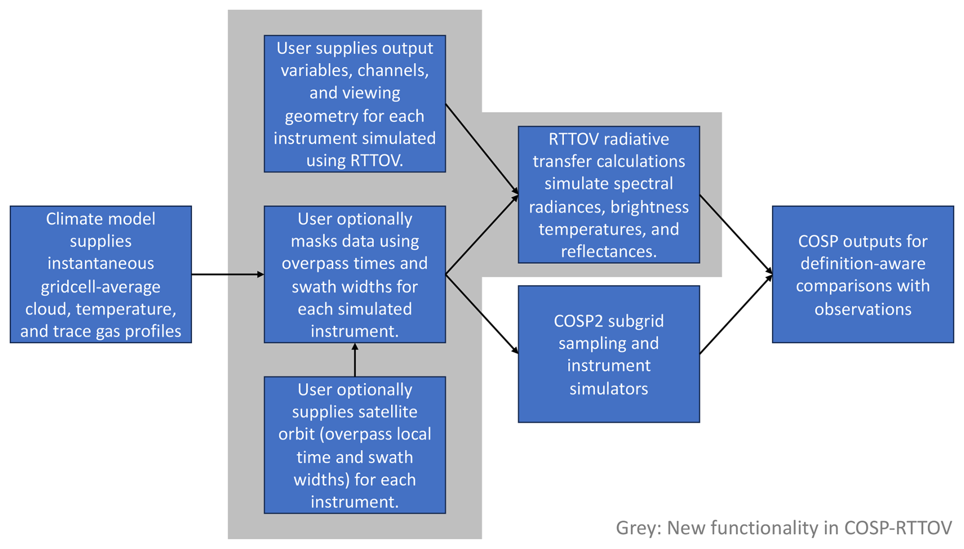
COSP-RTTOV adds the flexible simulation of spectral radiation fields to the functionality of COSP2 (Swales et al., 2018). As a secondary improvement, we also enable simple satellite-like sampling patterns for COSP2 retrievals. The simulation of spectrally resolved radiation fields is accomplished by coupling the RTTOV v13 radiative transfer model (Saunders et al., 2018) to COSP2. The addition of satellite-like sampling patterns is accomplished by limiting simulator calculations to grid cells that fall within user-specified viewing swaths. Figure 1 shows a simplified flowchart of COSP-RTTOV operations, with new functionality relative to COSP2 boxed in grey.

Figure 1 COSP-RTTOV schematic.

2.1 Flexible simulation of spectral radiation fields

2.1.1 Coupling with the RTTOV radiative transfer model

We use the RTTOV radiative transfer model to efficiently generate spectral radiation fields over the entire globe for century-scale ESM simulations. RTTOV is a fast radiative transfer model for simulating satellite radiances. RTTOV can account for the different spectral response functions of spectral channels on various instrument platforms, which is essential for enabling consistent comparisons with observations. For complete RTTOV documentation, we refer the reader to Saunders et al. (2018).

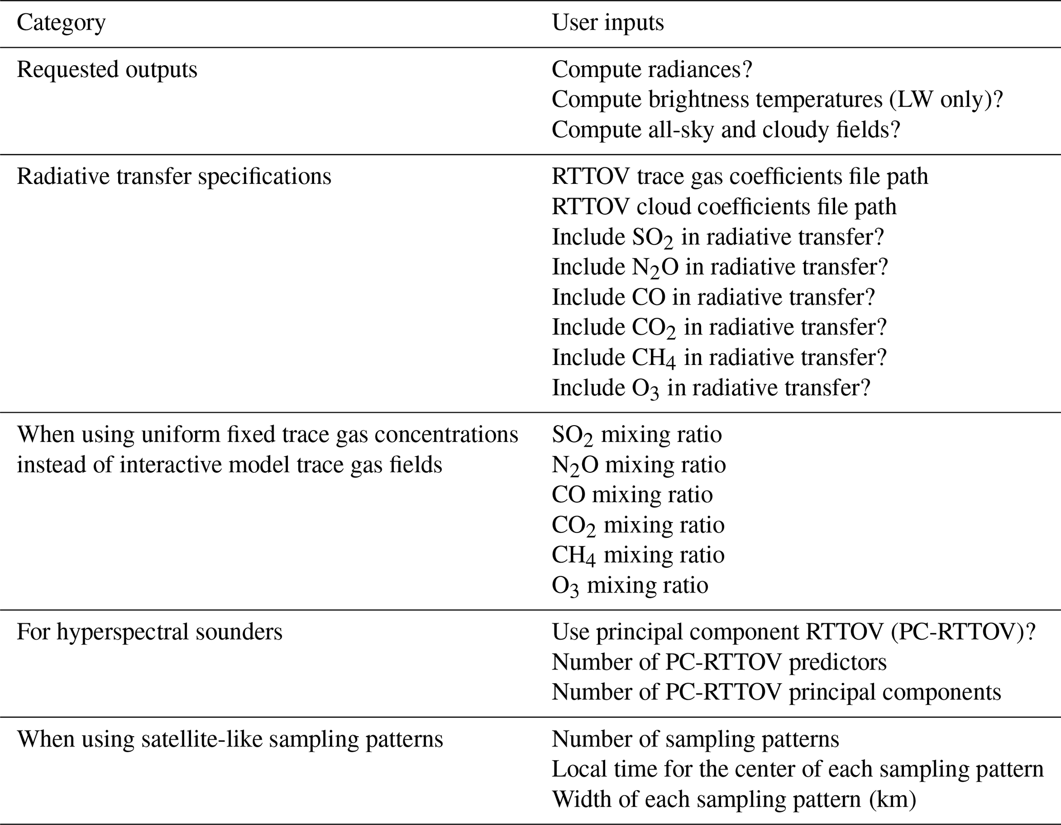
To produce spectral radiation fields, grid-cell-average surface properties and profiles of temperature, trace gas concentrations, and cloud properties are passed from an ESM to RTTOV via COSP. To determine which radiation fields are produced, users specify which subset of spectral channels and output fields should be produced for each instrument simulated by RTTOV. All user specifications available in COSP-RTTOV are summarized in Table 1.

Table 1 User specifications for instruments simulated in COSP-RTTOV.

2.1.2 Earth system model experiments with the Community Earth System Model Version 2 (CESM2) and COSP-RTTOV

We run multiple model experiments using CESM2 (Danabasoglu et al., 2020) as the host model for COSP-RTTOV. We use the single-column version of CESM2's atmospheric component (Gettelman et al., 2019) to validate the performance of COSP-RTTOV. We additionally use global atmosphere-only simulations to demonstrate the applications of COSP-RTTOV. All experiments use the CESM2.1.5 release.

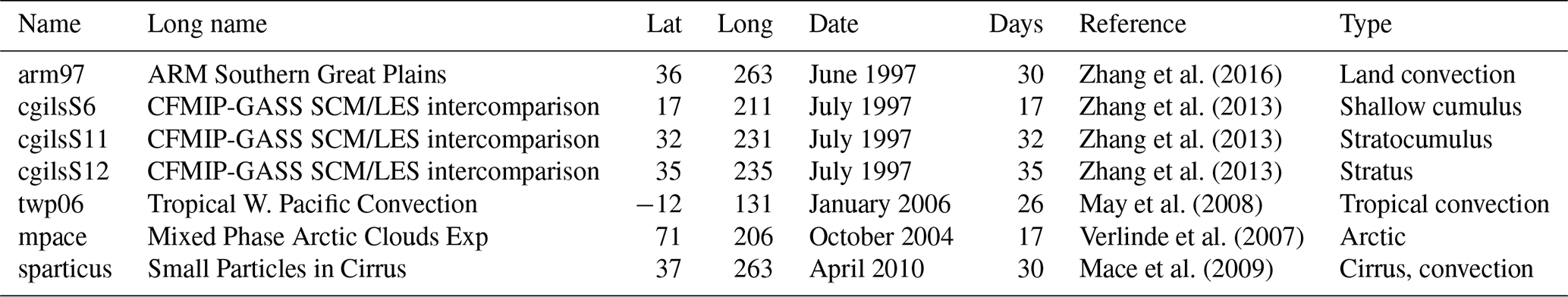
We run single-column experiments for seven Intensive Observation Period (IOP) cases that sample a wide variety of atmospheric and cloud conditions (Table 1 from Gettelman et al., 2019, is reproduced here as Table 2). IOPs range from 17 to 30 d, and all radiation fields are computed hourly. In these experiments, all-sky spectral irradiance fields are produced from CESM2's internal radiative transfer scheme for comparison with COSP-RTTOV (Sect. 2.1.4). CESM2 uses the Rapid Radiative Transfer Model longwave (RRTMG-LW) radiation scheme (Mlawer et al., 1997; Pincus et al., 2003), which divides longwave radiation into 16 spectral bands from 10 to 3250 cm⁻¹. When evaluating the clear-sky radiation fields produced by COSP-RTTOV, we use the arm97 IOP (Sect. 2.1.3).

Zhang et al. (2016)Zhang et al. (2013)Zhang et al. (2013)Zhang et al. (2013)May et al. (2008)Verlinde et al. (2007)Mace et al. (2009)

Table 2 Single-column model-intensive observation periods. Reproduced from Gettelman et al. (2019).

We run two global atmosphere-only experiments to compare with the observational satellite record and quantify internal climate variability. In both experiments, we simulate a subset of Atmospheric Infra-Red Sounder (AIRS) channels to limit the computational cost and the volume of data produced. The first experiment runs from 2000 to 2022 and uses observed sea surface temperatures and sea ice fields as boundary conditions. Atmospheric forcings are taken from the CMIP6 AMIP protocol from 2000 to 2014 and from the CMIP6 SSP3-7.0 scenario from 2015 to 2022. This experiment is intended to be compared with observations. The second experiment uses surface boundary conditions and atmospheric forcings from the CESM2 pre-industrial control experiment. Specifically, sea surface temperature and sea ice fields are taken from years 501 to 699 of the pre-industrial experiment. This experiment quantifies internal variability in an unforced pre-industrial climate for use in climate change detection studies.

2.1.3 Validation of clear-sky brightness temperatures against the Stand-alone AIRS Radiative Transfer Algorithm (SARTA)

The primary function of COSP-RTTOV is to produce synthetic radiance and brightness temperature fields that are consistent with satellite observations. We accomplish this by comparing COSP-RTTOV to a radiative transfer tool used by NASA's AIRS mission. SARTA (Strow et al., 2003, 2006; Desouza-Machado et al., 2020) is a fast radiative transfer model for simulating AIRS radiances, given realistic atmospheric profiles of water vapor, ozone, temperature, and other parameters such as surface emissivity.

SARTA's accuracy and wide spectral coverage make it an excellent validation tool for COSP-RTTOV. We specifically compare 2645 AIRS L1C channels. These spectral channels are corrected for drift and are shifted to a fixed-frequency grid, making them ideal for long-term comparisons. Figure 2 compares clear-sky brightness temperatures produced by COSP-RTTOV and SARTA for the arm97 IOP (Table 2). Overall, Fig. 2 demonstrates that COSP-RTTOV simulates accurate clear-sky radiation fields for comparisons with infrared sounders. Good agreement (mean error <1 K and error standard deviation <0.5 K) is shown for virtually all spectral regions. Larger differences in the 667–668 cm⁻¹ spectral region result from different assumptions about the atmospheric column above the CESM2 top between COSP-RTTOV and SARTA. Thus, discrepancies here are not relevant to the intended applications of COSP-RTTOV. Because COSP-RTTOV is intended for direct radiation comparisons and not geophysical retrievals, more detailed accounting of brightness temperature differences is not needed.

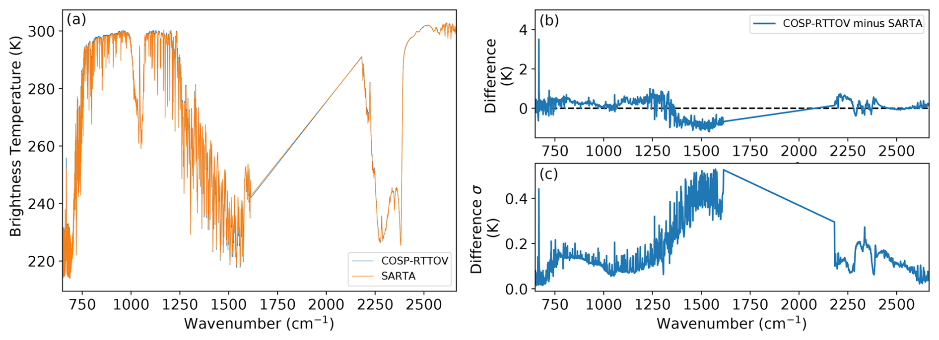
Figure 2 Comparison of brightness temperatures produced by COSP-RTTOV and SARTA for AIRS L1C channels. (a) Simulated brightness temperatures across the AIRS spectral region (3.7–15.4 µm). (b) Mean and (c) standard deviation of COSP-RTTOV brightness temperature differences relative to SARTA. Brightness temperatures are computed for 333 atmospheric profiles taken from a single-column mid-latitude simulation of COSP-RTTOV (see Sect. 2.1.4).

2.1.4 Validation of all-sky irradiance against CESM2 and RRTMG

We next validate COSP-RTTOV against the all-sky radiation fields produced by CESM2. A key goal of COSP2 was to allow for greater consistency between the cloud properties used in the host model and those used to produce COSP's diagnostic outputs. RTTOV, however, has its own schemes for cloud optics and cloud overlap assumptions (how clouds at different vertical levels are distributed at subgrid scales). Specifically, users may select cloud optics from multiple parameterizations and choose between maximum/random and simplified two-column cloud overlap schemes (Saunders et al., 2018). Effectively, this means that the speed of RTTOV calculations comes at the expense of not being able to ensure consistency with the host model.

To understand the influence of different radiative transfer assumptions about the radiative properties of clouds, we compare COSP-RTTOV with RRTMG-LW. To compare against spectral irradiance fields from RRTMG-LW, we produce RRTMG-like all-sky irradiances from COSP-RTTOV. These RRTMG-like irradiances are computed by simulating radiance fields at high spectral resolution for multiple viewing angles, summing over the appropriate spectral interval, and performing a quadrature over solid angle. Specifically, we use channels based on the spectral response functions of two Fourier transform spectrometer instruments, the Infrared Atmospheric Sounding Interferometer (IASI) and the Far-infrared Outgoing Radiation Understanding and Monitoring (FORUM) mission's interferometer. We simulate IASI-like channels to cover the 700–2600 cm⁻¹ region and FORUM-like channels to cover the 100–700 cm⁻¹ region. The IASI (FORUM) channels have 0.25(0.3) cm⁻¹ spacing and 0.5(0.5) cm⁻¹ resolution. This spectral range allows comparison with 14 of the 16 RRTMG-LW channels.

Comparing COSP-RTTOV with the RRTMG spectral irradiances requires simulation of tens of thousands of individual spectral channels at each time step for a single atmospheric column. Computing and saving this many additional output fields for every grid cell of an ESM is not computationally feasible, so we validate using single-column experiments. The single-column IOP cases (Table 2) allow us to confirm that COSP-RTTOV fields consistently represent the cloud properties of CESM2.

Figure 3 compares the RRTMG-LW and RRTMG-like all-sky irradiances for all single-column IOPs. Because COSP-RTTOV and RRTMG-LW see identical model states, differences between them result only from the models themselves and the conversion of COSP-RTTOV radiances into RRTMG-like irradiances. The total all-sky irradiance error summed across all of the bands never exceeds 3 W m⁻², and the total fractional error never exceeds 2 %. Fractional errors for individual spectral bands are larger but never exceed 10 % and are almost always less than 5 %. Because regional all-sky model biases are often greater than these values, we find this level of agreement to be appropriate for the intended applications of COSP-RTTOV. Furthermore, the presence of similar irradiance biases in an analogous clear-sky comparison (Fig. A1), despite strong agreement in clear-sky radiances with SARTA (Fig. A2), indicates that the radiance-to-irradiance conversion is likely the main source of error. Because COSP-RTTOV is intended for brightness temperature and radiance comparisons, we are confident that Fig. 3 indicates a conservative upper bound on all-sky errors. Overall, Figs. 2 and 3 demonstrate that COSP-RTTOV appropriately simulates satellite radiances and replicates the cloud properties of the host model.

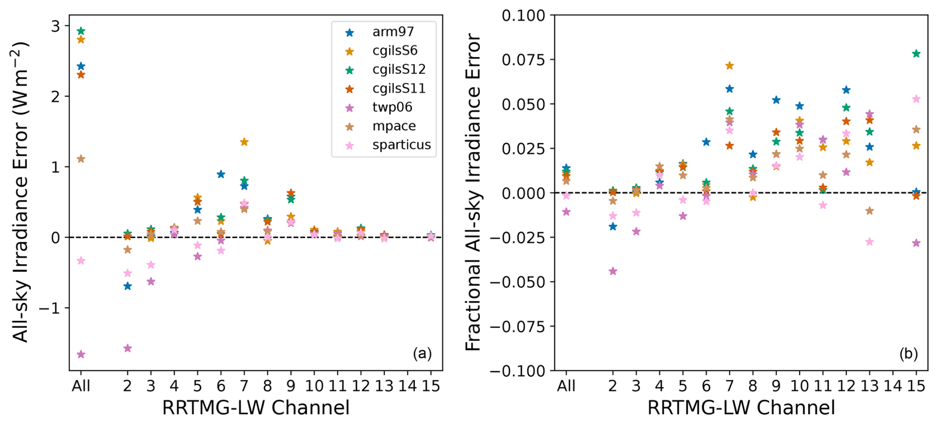
Figure 3 Comparison of all-sky irradiances produced by COSP-RTTOV and CESM2 for 14 spectral bands in RRTMG-LW. (a) Mean all-sky irradiance error. (b) Fractional all-sky irradiance error. Temporal averages are taken before comparison between COSP-RTTOV and RRTMG-LW. The spectral boundaries (cm⁻¹) for RRTMG-LW bands 2–15 are 350, 500, 630, 700, 820, 980, 1080, 1180, 1390, 1480, 1800, 2080, 2250, 2380, and 2600 (e.g., Band 3 spans 500–630 cm⁻¹). Band 14 samples the mesosphere above the CESM2 top and is excluded from this analysis. RTTOV radiances are converted to irradiances using a six-point Gaussian quadrature with viewing zenith angles and weights following Stamnes et al. (2017).

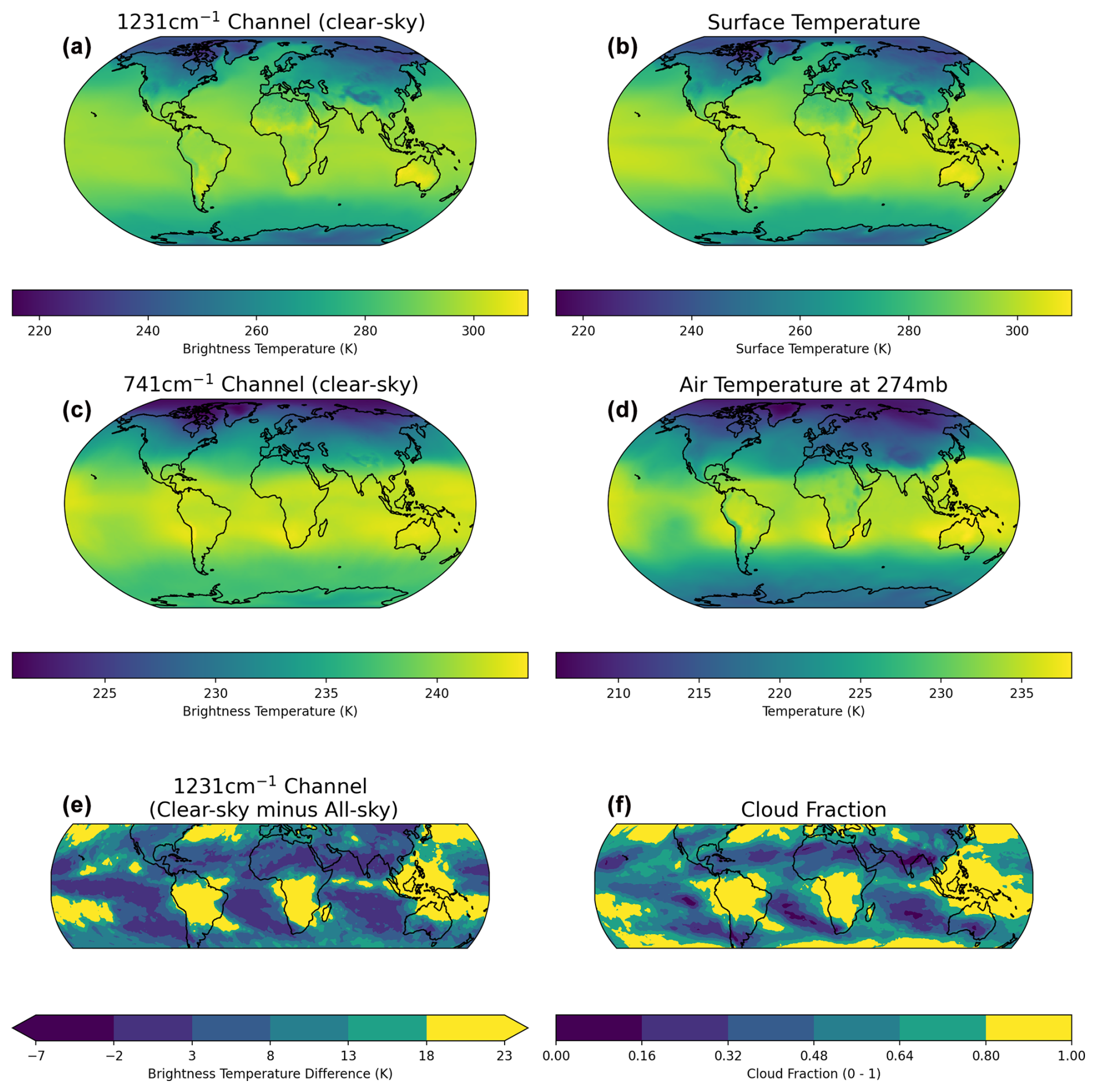
Figure 4 Comparison of COSP-RTTOV brightness temperatures and geophysical fields produced in a CESM2 historical simulation. (a) Clear-sky brightness temperatures for a transparent AIRS window channel at 1231.33 cm⁻¹. (b) Surface temperature. (c) Clear-sky brightness temperatures for an AIRS channel sensitive to upper-tropospheric temperature and CO₂ at 740.97 cm⁻¹. (d) Air temperature at 274 mb. (e) Difference between clear-sky and all-sky brightness temperatures in the 1231.33 cm⁻¹ AIRS window channel. (f) Total cloud fraction. Panels (e) and (f) are restricted to 60° S–60° N, where there is high thermal contrast between clouds and the surface. All of the panels represent average values for January 2000.

2.2 Satellite-like sampling patterns

To specify satellite-like sampling patterns, users may supply a list of sampling local times (h) and swath widths (km). The sampling “local time” refers to a linear shift from UTC as a function of a grid cell's longitude ($t_{\text{local}}=t_{\text{UTC}}-\text{longitude}\times \mathrm{24}/\mathrm{360}$). This specification mimics satellite overpass times and ensures consistent sampling of the diurnal cycle. Conversely, the “swath width” determines the spatial region around each local time that is simulated. Supplying a swath width in units of distance rather than radians produces a larger sampling density at higher latitudes that is consistent with observations. By specifying any number of sampling local times and swath widths, users can emulate output comparable to a single daytime or nighttime instrument or simulate an entire constellation of identical instruments with different orbits. Applying these sampling patterns also reduces computational cost because simulators are run only on a subset of grid cells (see Sect. 2.3). If sampling patterns are not specified, outputs are computed for all grid cells at each time step as in previous versions of COSP.

2.3 Computational cost

To quantify the computational cost of running COSP-RTTOV, we report the cost of global atmosphere-only CESM2 experiments with different COSP-RTTOV configurations. Table 3 describes each experiment and reports the computational cost. Simulating spectral fields using RTTOV is more expensive than running the standard COSP2 simulators. However, applying reasonable swathing patterns cuts these costs noticeably.

Table 3 Computational cost of COSP-RTTOV.

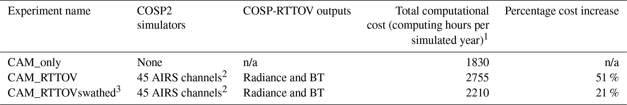
¹ CESM2 is run at 1° resolution in an atmosphere-only configuration using eight nodes in the NCAR Derecho system. ² Radiance fields are produced as clear-, cloudy-, and total-sky averages. Brightness temperatures are produced as clear- and total-sky averages. ³ Orbit centered at 13:30 local time with a 1800 km swath width. n/a: not available.

3 Simulator applications

Having described the simulator design and validation in Sect. 2, we now demonstrate the utility of global simulations of spectral radiation fields (Sect. 3.1) and satellite-like sampling patterns (Sect. 3.2).

3.1 Simulation of spectral radiation fields

3.1.1 Model evaluation

Evaluating models against direct radiation observations gives insight into model biases without the epistemic uncertainty present in geophysical retrievals or reanalysis products. To be valuable for model developers, however, radiation fields should be intuitively related to geophysical variables and climate processes. Figure 4 shows global maps of simulated brightness temperatures paired with the corresponding geophysical fields that they effectively capture. Clear-sky radiation in transparent spectral regions effectively measures surface temperatures (Fig. 4a and b). Similarly, a channel sensitive to the upper troposphere strongly resembles 274 mb temperatures (Fig. 4c and d). Finally, simple radiation comparisons can also capture cloud fields in regions with high thermal contrast (Fig. 4e and f). Overall, Fig. 4 demonstrates that appropriately chosen spectral channels enable ESM evaluation against direct observables without the loss of physical intuition often associated with radiation fields.

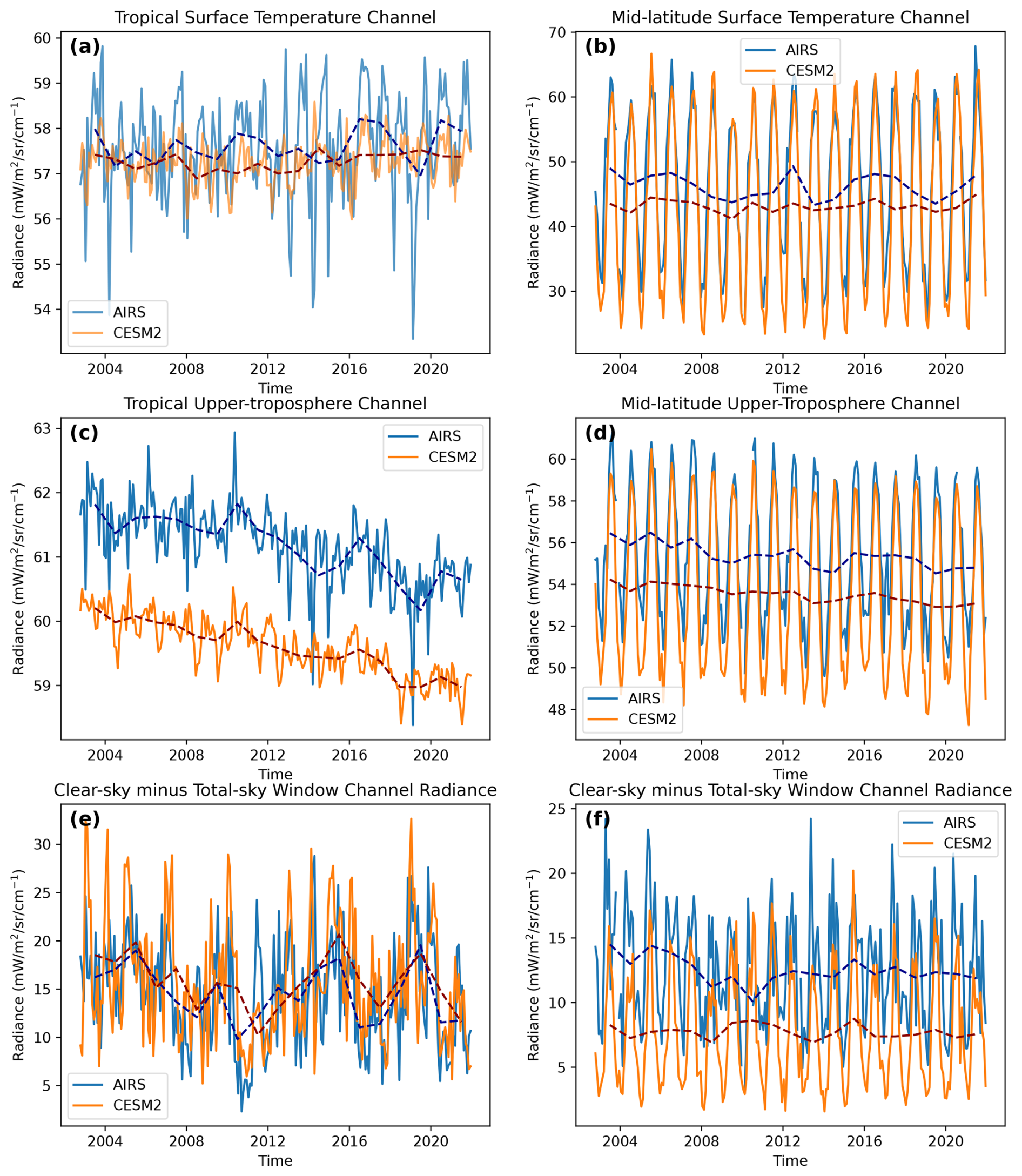
Figure 5 Evaluation of CESM2 against radiation time series using COSP-RTTOV. The rows show different spectral channels sampling surface temperatures, the upper troposphere, and clouds as described in Fig. 4. Panels (a), (c), and (e) show results from a region in the tropical Pacific (0–2.75° N, 160–165° E). Panels (a), (c), and (e) show results over a land region in North America (44–46.75° N, 95–100° E).

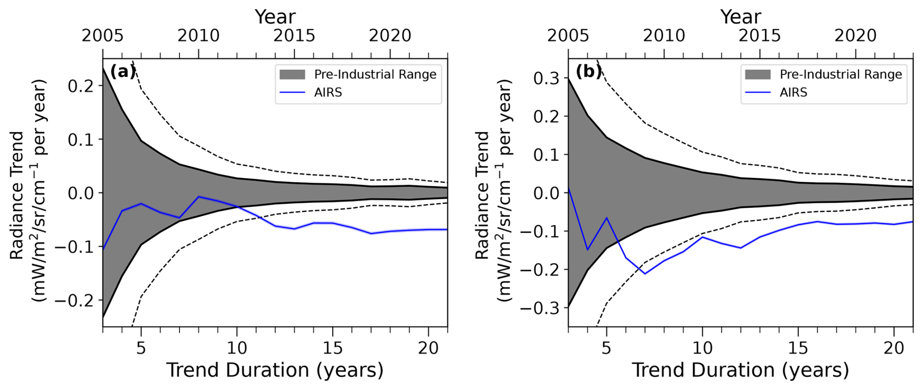
Figure 6 Time of emergence of radiance trends for the AIRS 740.97 cm⁻¹ channel sampling the upper troposphere. Panels (a) and (b) show results from regions in the tropical Pacific (0–2.75° N, 160–165° E) and North America (44–46.75° N, 95–100° E), respectively. The blue lines show trends in AIRS radiances. The trends begin in 2005 when 3 years of data were available (2003–2005). The grey-shaded regions span a 95 % confidence interval on unforced trends calculated from a 199-year CESM2 pre-industrial control simulation following the methods of Shaw and Kay (2023) and Shaw and Lenssen (2024). The dotted grey lines double CESM2's estimate of internal variability given the possibility that CESM2 underestimates regional variability. The AIRS record emerges from internal variability when it exits and remains outside the envelope of internal variability.

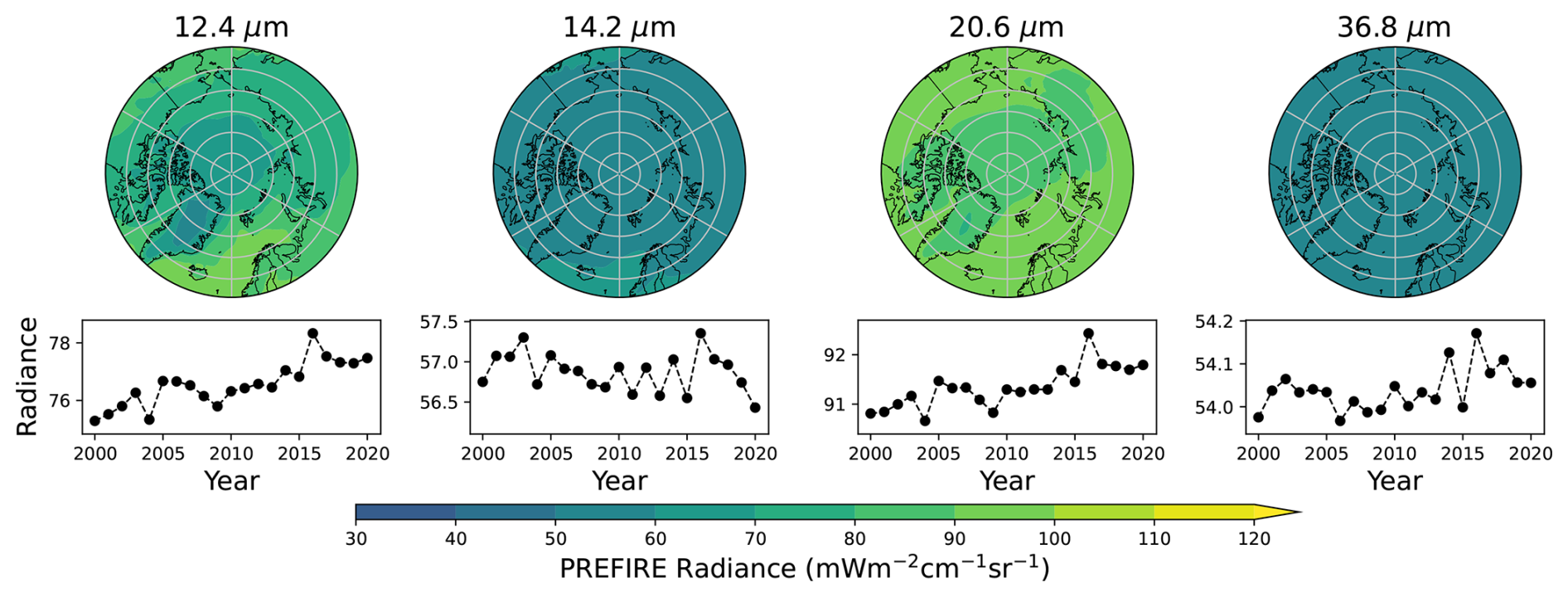
Figure 7 Top row: polar maps of mean simulated radiances for PREFIRE channels at 12.4, 14.2, 20.6, and 36.8 µm over the 1979–2014 period. Bottom row: time series of annual mean radiance values averaged over 60–90° N show the combined effects of forced change and internal climate variability.

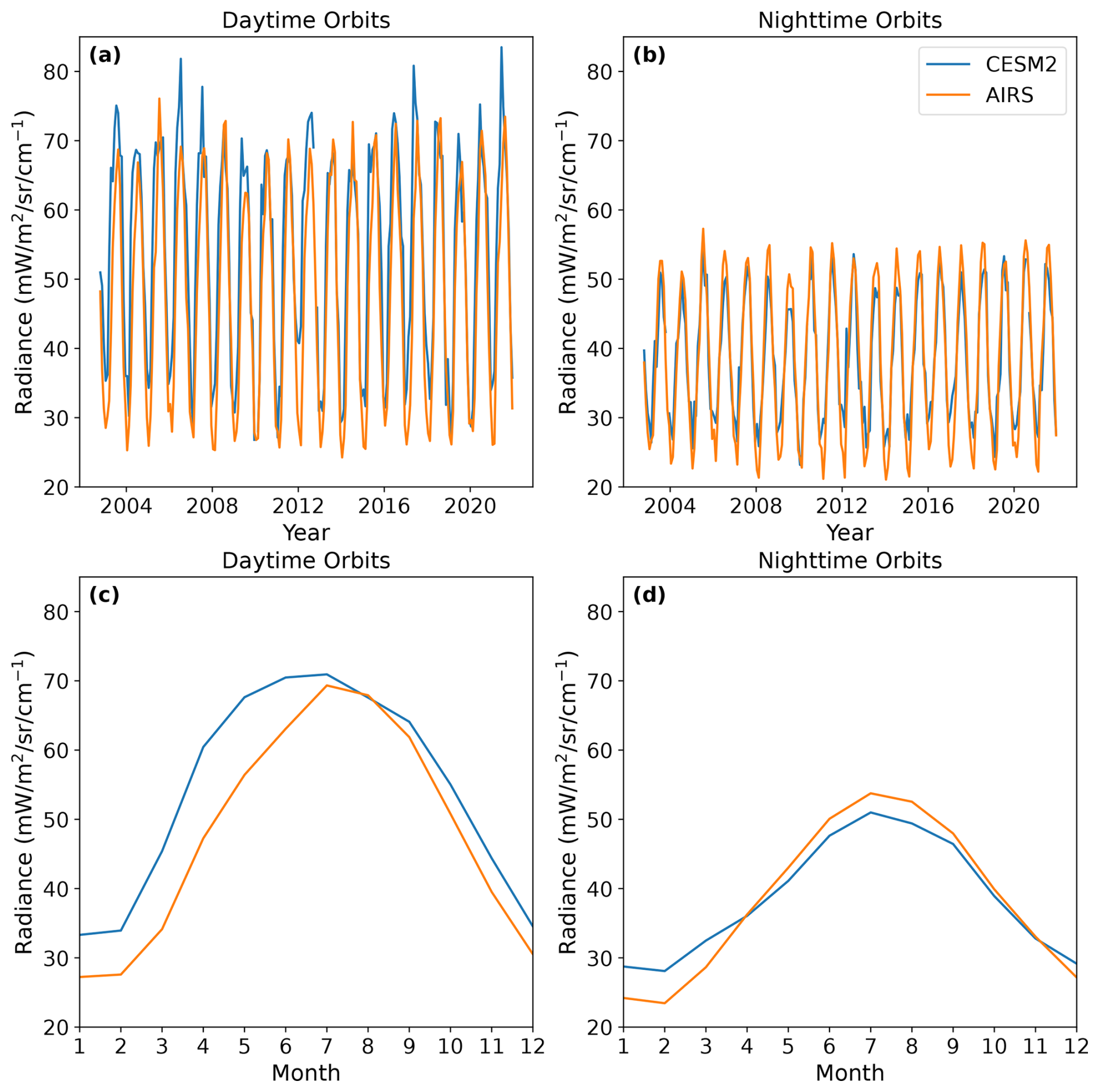
Figure 8 Comparison of AIRS and CESM2 for clear-sky radiances at 1231 cm⁻¹ for a land region in North America (44–46.75° N, 95–100° E) for ascending orbits (13:30 local time) and descending orbits (01:30 local time). (a) Monthly time series for ascending orbits. (b) Monthly time series for descending orbits. (c) Monthly climatology for ascending orbits. (d) Monthly climatology for descending orbits.

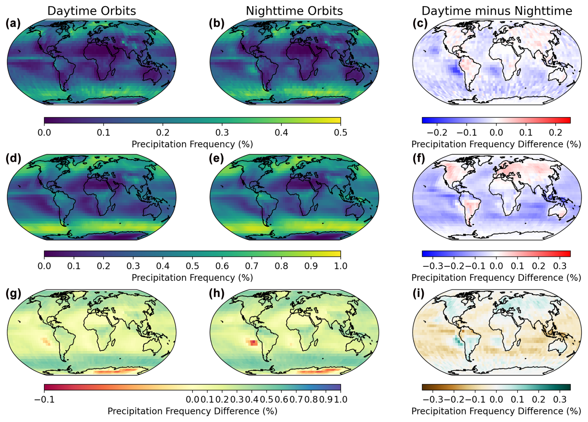
Figure 9 Comparison of daytime and nighttime precipitation frequencies from CloudSat and the COSP CloudSat simulator run in CESM2. (a) Observed precipitation frequency for daytime (13:30 local time) orbits. (b) Observed precipitation frequency for nighttime (01:30 local time) orbits. (c) Observed daytime minus nighttime precipitation frequency. (d–f) Precipitation frequency as in panels (a)–(c) but from CESM2. (g–i) Precipitation frequency as in panels (a)–(c) but from CESM2 minus CloudSat observations. CloudSat observations and CESM2 output are averaged from June 2006 through May 2010. Note that the color bars in the top two rows have different ranges. CloudSat observations use Haynes et al. (2009) and Smalley et al. (2014). The modeled output uses the COSP CloudSat simulator (Kay et al., 2018).

Once the relationships between radiation fields and geophysical variables have been established, we can easily evaluate the model performance. Figure 5 compares the COSP-RTTOV output with observed AIRS radiances from the same spectral channels shown in Fig. 4. Results are shown for a tropical region in the equatorial Pacific (left column) and a land surface at the mid-latitudes (right column). This comparison identifies a wintertime cold bias at the mid-latitudes (Fig. 5b). The upper-tropospheric channel (Fig. 5c and d) shows both a cold bias and a secular cooling trend, in agreement with the AIRS observations. Finally, the simple cloud amount metric in Fig. 5e demonstrates that CESM2 captures the interannual variability from AIRS observations.

3.1.2 Climate change detection

In addition to providing a strict constraint on model performance, COSP-RTTOV enables the use of radiation records in studies on climate change detection and attribution. Specifically, centennial-scale pre-industrial control simulations can characterize internal climate variability in radiation fields (e.g., Shaw and Kay, 2023). Distinguishing observed change from this internal variability enables the attribution of observed changes to anthropogenic forcing. Figure 6 compares observed AIRS radiance trends with internal variability generated from a pre-industrial control simulation run with COSP-RTTOV. Specifically, we examine the signal of CO₂ increase in the upper-tropospheric channel in Fig. 5c and d. For both tropical and mid-latitude regions, AIRS detects a forced change within 15 years. The observed cooling trend is the result of increasing CO₂ concentrations and upper-tropospheric temperature change. Increased CO₂ concentrations raise thermal emissions to higher and colder pressure levels, which themselves are also cooling. By producing satellite-like radiation fields from a long pre-industrial control simulation using COSP-RTTOV, this approach can be flexibly applied to multiple spectral channels and spatial regions.

3.1.3 OSSEs

COSP-RTTOV allows us to easily run climate OSSE experiments for evaluating proposed missions and placing short satellite missions into the broader context of forced change and internal climate variability. Figure 7 shows one example using the recently launched NASA PREFIRE mission (L'Ecuyer et al., 2021). Climatological averages of PREFIRE-like radiances (Fig. 7, top row) are computed by running COSP-RTTOV in historical ESM simulations. Additionally, annual time series from the same ESM experiment quantify forced change and internal variability (Fig. 7, bottom row). While PREFIRE channels centered at 12.4 and 14.2 µm, respectively, sample the atmospheric window and CO₂ absorption, additional channels at 20.6 and 36.8 µm sample features in the previously unobserved far-infrared. Evaluating PREFIRE observations against this synthetic record allows differences resulting from model physics to be separated from internal climate variability. Overall, producing PREFIRE-like radiances with COSP-RTTOV in long historical simulations provides a longer context in which to interpret a short observational record.

3.2 Satellite-like sampling patterns

While producing satellite-like radiation fields is the main function of COSP-RTTOV, the implementation of satellite-like sampling patterns also enables new science applications.

3.2.1 Separate evaluation of ascending and descending orbit branches

Sun-synchronous satellites make observations at two distinct times of the day, allowing for investigations of both daytime and nighttime fields. Comparisons with ESMs, however, often only study the average field and lose the benefits of diurnal sampling. Figure 8 shows a comparison of both daytime and nighttime AIRS radiances for a surface temperature channel for a mid-latitude region. This comparison reveals that CESM2's wintertime cold bias occurs throughout the day, while compensating biases during the summer (overly cold days and overly warm nights) lead to good agreement on average. Comparing averages over all orbits (e.g., Fig. 5b) does not provide this insight. Satellite-like sampling in COSP-RTTOV enables these comparisons without saving high-frequency model output or running offline radiative transfer models.

3.2.2 Quantification of sampling biases

COSP-RTTOV's diurnal sampling patterns can also be applied to standard COSP2 outputs. We demonstrate one application to precipitation frequency as observed by CloudSat, a spaceborne radar that flew from 2006 to 2023 measuring cloud structure and precipitation (Stephens et al., 2008). Figure 9a and b show the observed precipitation frequency from CloudSat for daytime and nighttime orbits (Haynes et al., 2009; Smalley et al., 2014). The diurnal contrast (Fig. 9c) shows that precipitation frequency is generally highest over the ocean surface during the day and over the land surface during the night. Using COSP-RTTOV satellite-like sampling and COSP's CloudSat simulator (Kay et al., 2018), we generate comparable fields from CESM2 (Fig. 9d–f). Qualitatively, CESM2 produces spatial patterns of precipitation frequency that closely resemble CloudSat. Differences between the simulated and observed fields (Fig. 9g and h), however, show that CESM2 has overly frequent precipitation during both daytime and nighttime orbits, leading to an overestimation of the diurnal contrast in precipitation frequency (Fig. 9i). Over stratocumulus regions west of tropical continents, however, CESM2 completely misses the observed diurnal precipitation pattern. CloudSat shows a greater nighttime precipitation frequency (Fig. 9c), while CESM2 has near-zero diurnal contrast (Fig. 9f). We emphasize that these comparisons require both consistent definitions of retrieved fields (provided by individual satellite simulator modules) as well as consistent definitions of their spatiotemporal sampling (provided by COSP-RTTOV). The large diurnal precipitation contrast also demonstrates that fair comparisons with the CloudSat record following the 2011 battery anomaly (after which CloudSat only observed daytime scenes) require appropriate sampling patterns.

4 Conclusions

We developed a flexible and computationally efficient tool for simulating satellite-like radiation fields within Earth system models. COSP-RTTOV is broadly applicable to satellite radiation fields in both clear and cloudy scenes. Furthermore, the satellite-like radiation fields produced by COSP-RTTOV are consistent with instrument spectral response functions and orbit sampling as well as the internal physics of the host model. The definition- and scale-aware comparisons enabled by COSP are thus broadly extended to studies using spectral infrared satellite observations. COSP-RTTOV emulates direct satellite observations that are tied to standards with known uncertainties. Evaluating ESMs against direct radiation observations is thus a strong test of their performance, and COSP-RTTOV is a single tool that enables such comparisons. Here, we have described the design, validation, and potential uses of COSP-RTTOV. We demonstrate applications for short satellite missions, ESM evaluation, and climate change detection. Collectively, these examples demonstrate that COSP-RTTOV is a valuable tool for the modeling and observational communities. We welcome contributions of the broader community to further improvements to COSP-RTTOV.

Appendix A

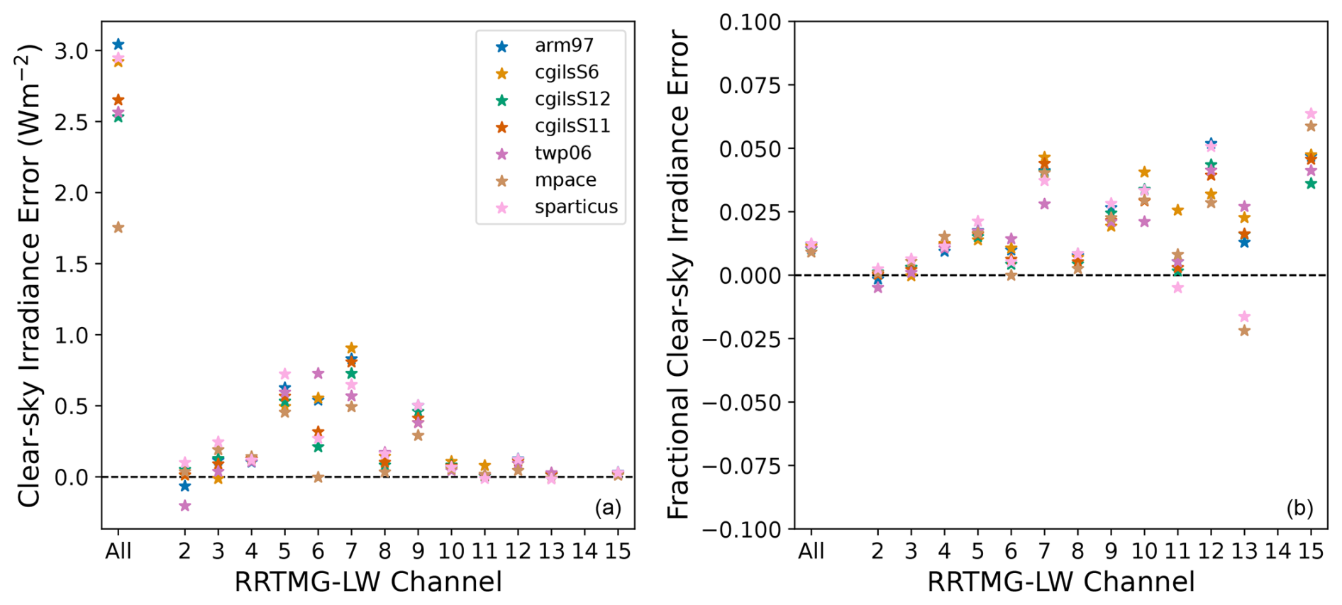
Figure A1 Comparison of clear-sky irradiances produced by COSP-RTTOV and CESM2 for 14 spectral bands in RRTMG-LW. (a) Mean clear-sky irradiance error. (b) Fractional clear-sky irradiance error. Temporal averages are taken before comparison between COSP-RTTOV and RRTMG-LW. The spectral boundaries (cm⁻¹) for RRTMG-LW bands 2–15 are 350, 500, 630, 700, 820, 980, 1080, 1180, 1390, 1480, 1800, 2080, 2250, 2380, and 2600 (e.g., Band 3 spans 500–630 cm⁻¹). Band 14 samples the mesosphere above the CESM2 top and is excluded from this analysis. RTTOV radiances are converted to irradiances using a six-point Gaussian quadrature with viewing zenith angles and weights following Stamnes et al. (2017).

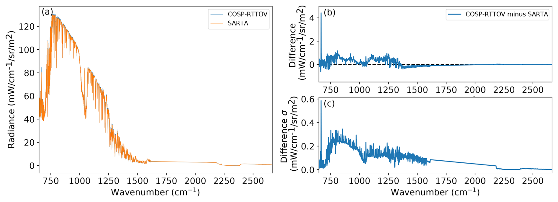
Figure A2 Comparison of radiances produced by COSP-RTTOV and SARTA for the AIRS L1C channels. (a) Simulated radiances across the AIRS spectral region (3.7–15.4 µm). (b) Mean and (c) standard deviation of COSP-RTTOV radiance differences relative to SARTA. Radiances are computed for 333 atmospheric profiles taken from a single-column mid-latitude simulation of COSP-RTTOV (see Sect. 2.1.4).