Stabilized two-phase material point method for hydromechanical coupling problems in solid–fluid porous media

For the hydromechanical coupling of solid–fluid porous media, this study presents an explicit stabilized two-phase material point method (MPM) formulation based on the one-point two-phase MPM scheme. To mitigate the spurious pore pressure and maintain the numerical stability, stabilized techniques, including the strain smoothing method and the multi-field variational principle, are implemented in the proposed formulation. The strain smoothing technique is used to smooth the volumetric strain rate, and the calculation of the pore pressure increment at particles is based on the multi-field variational principle. Four numerical examples are performed to evaluate the performance of the proposed formulation. With its effective and easy-to-implement stabilized techniques, the proposed formulation provides stable and reliable outcomes that align well with analytical solutions and results from other approaches, offering extensive validation that the proposed two-phase MPM formulation is an effective and reliable approach for the simulation of solid–fluid porous media under both static and dynamic conditions.

1 Introduction

The hydromechanical coupling of solid–fluid porous media widely presents in nature and engineering, from natural processes such as rainfall-induced landslide and earthquake-induced liquefaction to coastal dike-breaking and offshore foundations (Jerolmack and Daniels, 2019; Zhan et al., 2025; Guan and Shi, 2023). Due to the practical importance, reproducing and understanding the physical nature of such a two-phase system has attracted strong research interests across many scientific and engineering disciplines and has become increasingly recognized with recent advances in both observational and simulation tools (Li et al., 2023; Taylor-Noonan et al., 2022; Pudasaini and Mergili, 2019). Numerical modeling of this two-phase coupling system is of great interest in geological hazard prevention and in the geotechnical field, yet it remains a significant challenge for researchers in many disciplines alike.

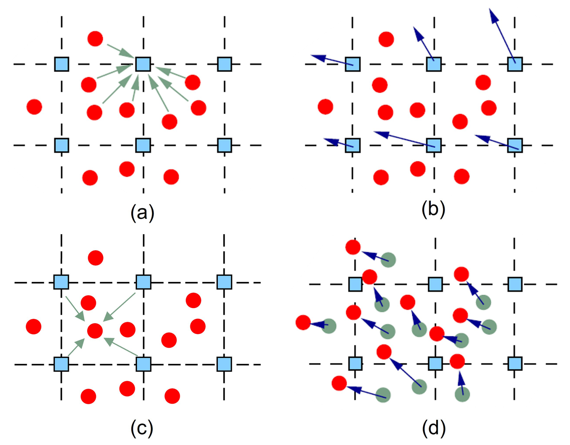
Figure 1 Standard algorithm of MPM: (a) interpolating information from particles to nodes, (b) solving governing equations on nodes, (c) interpolating information from nodes to particles, (d) updating particle information.

In solid–fluid-coupling problems, the motion of each constituent is governed by stress distributions, external gravity forces, and interaction forces (Pudasaini and Mergili, 2019; Baumgarten and Kamrin, 2018; Bandara and Soga, 2015). For the simulation of this two-phase system, various numerical methods have been proposed, including the smoothed particle hydrodynamics (SPH) method (Lian et al., 2023; Chen et al., 2023), the particle finite element method (FEM; Yuan et al., 2022; Jin and Yin, 2022), and the material point method (MPM) (Bandara and Soga, 2015; Bandara et al., 2016; Jassim et al., 2013; Yerro et al., 2015; Wyser et al., 2020). Among these methods, MPM has proven to be both effective and efficient for simulating large-deformation problems with history-dependent materials. Originating from the particle-in-cell (PIC) method, MPM is a hybrid Euler–Lagrangian method that has significant advantages in dealing with large-deformation problems (Li et al., 2020; Zhao et al., 2023; Fernández et al., 2023). In MPM, a continuum body is discretized by a group of material points carrying all physical information, such as displacement, velocity, stress, and strain. At each time step, the physical information at particles is interpolated to the background mesh, which is essentially Eulerian mesh; then, the governing equations can be solved on it. Subsequently, the solution is re-interpolated to each material particle for the update of particle physical information. The original background mesh can be used again in the new time step, which can eliminate the mesh distortion problem in the Lagrangian method, and the accuracy of large-deformation-problem simulations can be guaranteed (Fig. 1). Currently, various coupling MPM formulations have been proposed, i.e., the one-point or two-point schemes (Bandara and Soga, 2015; Jassim et al., 2013), the solid displacement–fluid pressure or solid velocity–fluid velocity formulation (Zhang et al., 2009; Lei et al., 2020) and have been widely used in two-phase coupling problems and engineering applications (Du et al., 2023; Ceccato et al., 2024; Shen et al., 2024; Zheng et al., 2024a; Yamaguchi et al., 2023; Zheng et al., 2024b; Zhan et al., 2025).

However, the standard MPM formulation usually employs lower-order shape functions within an explicit time integration scheme for simplicity and efficiency, which suffers from the cell-crossing error and the volumetric locking when applied to coupled hydromechanical problems (Li et al., 2024; Sang et al., 2024). The cell-crossing error during particle movement arises from the use of lower-order shape functions, which exhibit discontinuous gradients between background mesh elements. To address this issue, higher-order interpolation functions with continuous gradients across elements can be employed, such as the Generalized Interpolation Material Point (GIMP) method (Bardenhagen and Kober, 2004), the B-spline method (De Vaucorbeil et al., 2020), and the Convected Particle Domain Interpolation (CPDI) (Wang et al., 2023b). Due to the low compressibility of pore fluid and limited permeability, the volumetric locking and erroneous strain may occur during simulation, which may not only result in undesired pore pressure oscillation but also render the simulation highly unstable. Various numerical stabilization techniques have been implemented in MPM to solve this issue, including the reduce integration (Bandara and Soga, 2015; Zheng et al., 2021), the B-bar approach (Wang et al., 2018; Tang et al., 2024), the nodal or cell smoothing method (Lei et al., 2020; Wang et al., 2023a), the fractional step method (Kularathna et al., 2021; Jassim et al., 2013), the polynomial pressure projection method (Zhao and Choo, 2020), the multi-field variational principle (Liu et al., 2020; Zheng et al., 2021; Tang et al., 2024; Zheng et al., 2022), and coupling with other algorithms (Baumgarten et al., 2021; Li et al., 2024; Tran et al., 2023; Sang et al., 2024). Although these techniques produce results that overcome volumetric locking and reduce pore pressure oscillation, some are conditionally stable and some require significant modifications of the existing MPM algorithm, leading to additional computation cost and difficulty (Lei et al., 2020; Li et al., 2024). Therefore, their usage should depend on the specific problem at hand. More features and limitations of these techniques can be found in the summaries of Li et al. (2024) and Sang et al. (2024).

Here, based on the one-point two-phase MPM scheme (Jassim et al., 2013), we propose an explicit stabilized two-phase MPM formulation for both static and dynamic analyses of solid–fluid porous media. To avert the volumetric locking and maintain the numerical stability, the stabilized techniques, including the strain smoothing method (Mast et al., 2012) and the multi-field variational principle (Chen et al., 2018), have been implemented in the proposed formulation. The strain smoothing method is employed to smooth the volumetric strain rate, and the calculation of the pore pressure increment at particles is based on the multi-field variational principle for accuracy and stability. The spurious pore pressure oscillation can be well mitigated during pore pressure calculation and interpolation. With these effective and easy-to-implement techniques, the volumetric locking can be significantly eliminated under both static and dynamic conditions. The study is organized as follows. Firstly, the governing equations for solid–fluid two-phase systems are briefly introduced in Sect. 2. The numerical implementation of the proposed formulation and the stabilized techniques are presented in Sect. 3; then, four numerical examples for the verification of the proposed method are performed and analyzed in Sect. 4. Finally, the last section contains the discussion and conclusions.

2 Governing equations

In one-point two-phase MPM formulation, according to the theory of mixture (Baumgarten and Kamrin, 2018), the representative volume (RVE) V_p of a particle material particle is a summation of solid-phase volume V_sp and fluid-phase volume V_fp, and each phase (solid, fluid) in the RVE can be characterized by its volume fraction (Fig. 2). The apparent density of each phase is characterized by the intrinsic density with the volume fraction, which reads

$$\begin{array}{}\text{(1)}& {\stackrel{\mathrm{‾}}{\mathit{\rho }}}_{\mathrm{s}}=\mathit{\phi }{\mathit{\rho }}_{\mathrm{s}},{\stackrel{\mathrm{‾}}{\mathit{\rho }}}_{\mathrm{f}}=n{\mathit{\rho }}_{\mathrm{f}},\end{array}$$

where φ is the solid volume fraction; n is the porosity; ρ_s and ρ_f are the intrinsic density of solid and fluid, respectively; and ${\stackrel{\mathrm{‾}}{\mathit{\rho }}}_{\mathrm{s}}$ and ${\stackrel{\mathrm{‾}}{\mathit{\rho }}}_{\mathrm{f}}$  are the apparent density of solid and fluid, respectively.

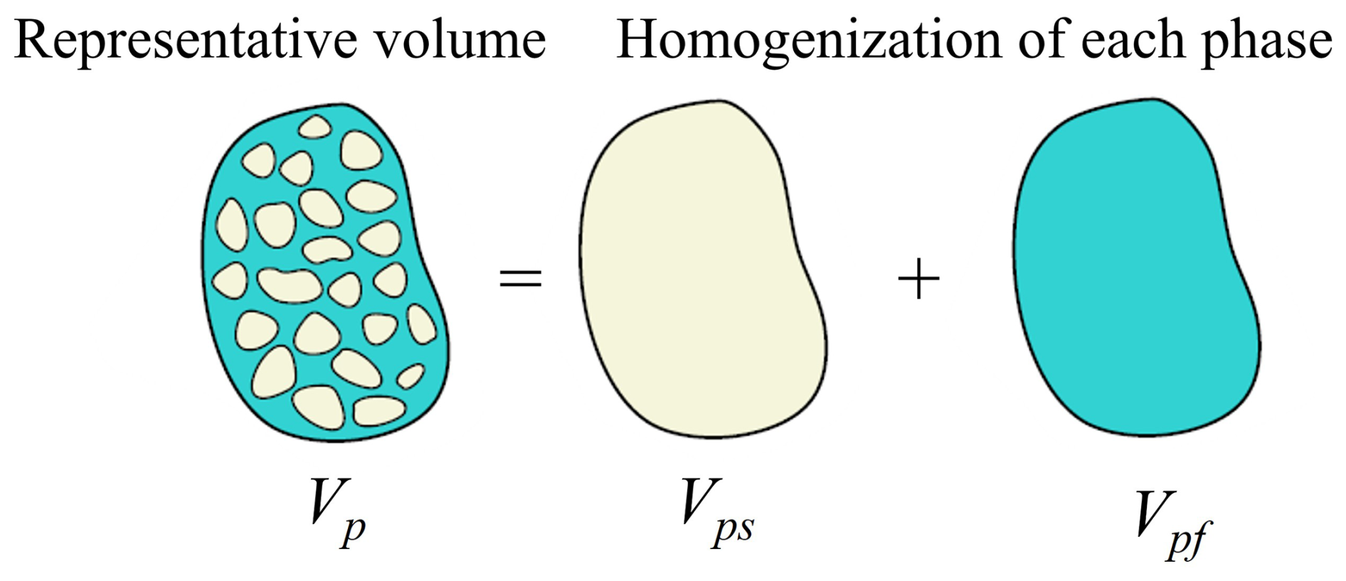
Figure 2 Sketch of material point composition in a single-point two-phase MPM model (Kularathna et al., 2021).

2.1 Mass conservation equations

The mass conservations in a part of the solid–fluid-phase continuum in Lagrangian description are expressed as

$$\begin{array}{}\text{(2)}& {\displaystyle }& {\displaystyle \frac{D^{\mathrm{s}}{\stackrel{\mathrm{‾}}{\mathit{\rho }}}_{\mathrm{s}}}{Dt}}+{\stackrel{\mathrm{‾}}{\mathit{\rho }}}_{\mathrm{s}}\mathrm{\nabla }\cdot {\mathit{v}}_{\mathrm{s}}=\mathrm{0},\text{(3)}& {\displaystyle }& {\displaystyle \frac{D^{\mathrm{f}}{\stackrel{\mathrm{‾}}{\mathit{\rho }}}_{\mathrm{f}}}{Dt}}+{\stackrel{\mathrm{‾}}{\mathit{\rho }}}_{\mathrm{f}}\mathrm{\nabla }\cdot {\mathit{v}}_{\mathrm{f}}=\mathrm{0},\end{array}$$

where v_s and v_f are the velocity of solid and fluid phases in their reference frames, respectively. In microscale, the solid grain is assumed to be incompressible, so ρ_s is constant. However, ${\stackrel{\mathrm{‾}}{\mathit{\rho }}}_{\mathrm{s}}$ will change when the solid phase compacts or dilates due to the deformation of the solid skeleton structure. Therefore, a simple expansion of Eq. (2) using the definition of porosity yields an expression for the change rate of the local measure of porosity,

$$\begin{array}{}\text{(4)}& {\displaystyle \frac{D^{\mathrm{s}}n}{Dt}}=(\mathrm{1}-n)\mathrm{\nabla }\cdot {\mathit{v}}_{\mathrm{s}}.\end{array}$$

In one-point two-phase MPM formulation, all constituents are represented by the same Lagrangian material point in the current configuration. The material time derivative of the fluid phase with respect to the motion of the solid phase is described as follows:

$$\begin{array}{}\text{(5)}& {\displaystyle \frac{D^{\mathrm{f}}}{Dt}}={\displaystyle \frac{D^{\mathrm{s}}}{Dt}}+({\mathit{v}}_{\mathrm{f}}-{\mathit{v}}_{\mathrm{s}})\cdot \mathrm{\nabla },\end{array}$$

so Eq. (3) can be expressed as

$$\begin{array}{}\text{(6)}& {\displaystyle \frac{D^{\mathrm{s}}{\stackrel{\mathrm{‾}}{\mathit{\rho }}}_{\mathrm{f}}}{Dt}}+({\mathit{v}}_{\mathrm{f}}-{\mathit{v}}_{\mathrm{s}})\cdot \mathrm{\nabla }{\stackrel{\mathrm{‾}}{\mathit{\rho }}}_{\mathrm{f}}+{\stackrel{\mathrm{‾}}{\mathit{\rho }}}_{\mathrm{f}}\mathrm{\nabla }\cdot {\mathit{v}}_{\mathrm{f}}=\mathrm{0},\end{array}$$

and Eq. (6) can be further written as

$$\begin{array}{}\text{(7)}& n{\displaystyle \frac{D^{\mathrm{s}}{\mathit{\rho }}_{\mathrm{f}}}{Dt}}+{\mathit{\rho }}_{\mathrm{f}}{\displaystyle \frac{D^{\mathrm{s}}n}{Dt}}+({\mathit{v}}_{\mathrm{f}}-{\mathit{v}}_{\mathrm{s}})\cdot \mathrm{\nabla }n{\mathit{\rho }}_{\mathrm{f}}+n{\mathit{\rho }}_{\mathrm{f}}\mathrm{\nabla }\cdot {\mathit{v}}_{\mathrm{f}}=\mathrm{0}.\end{array}$$

Assuming the fluid phase is barotropic, density variation in a barotropic fluid obeys the following relationship:

$$\begin{array}{}\text{(8)}& {\displaystyle \frac{\mathrm{1}}{{\mathit{\rho }}_{\mathrm{f}}}}{\displaystyle \frac{D^{\mathrm{s}}{\mathit{\rho }}_{\mathrm{f}}}{Dt}}={\displaystyle \frac{\mathrm{1}}{K_{\mathrm{f}}}}{\displaystyle \frac{D^{\mathrm{s}}{p}_{\mathrm{f}}}{Dt}},\end{array}$$

where K_f is the bulk modulus of fluid and p_f is the pore fluid pressure.

Combined with Eq. (4) and neglecting spatial variations in density and porosity, the pore pressure change rate can be obtained:

$$\begin{array}{}\text{(9)}& {\displaystyle \frac{D^{\mathrm{s}}{p}_{\mathrm{f}}}{Dt}}=-{\displaystyle \frac{K_{\mathrm{f}}}{n}}\left[\right(\mathrm{1}-n)\mathrm{\nabla }\cdot {\mathit{v}}_{\mathrm{s}}+n\mathrm{\nabla }\cdot {\mathit{v}}_{\mathrm{f}}].\end{array}$$

2.2 Momentum conservation equations

The momentum conservation equations for each continuum phase are given as

$$\begin{array}{}\text{(10)}& {\displaystyle }& {\displaystyle }{\stackrel{\mathrm{‾}}{\mathit{\rho }}}_{\mathrm{s}}{\displaystyle \frac{D^{\mathrm{s}}{\mathit{v}}_{\mathrm{s}}}{Dt}}={\stackrel{\mathrm{‾}}{\mathit{\rho }}}_{\mathrm{s}}\mathit{b}-f_{\mathrm{b}}-f_{\mathrm{d}}+\mathrm{\nabla }\cdot {\mathit{\sigma }}_{\mathrm{s}},\text{(11)}& {\displaystyle }& {\displaystyle }{\stackrel{\mathrm{‾}}{\mathit{\rho }}}_{\mathrm{f}}{\displaystyle \frac{D^{\mathrm{f}}{\mathit{v}}_{\mathrm{f}}}{Dt}}={\stackrel{\mathrm{‾}}{\mathit{\rho }}}_{\mathrm{f}}\mathit{b}+f_{\mathrm{b}}+f_{\mathrm{d}}+\mathrm{\nabla }\cdot {\mathit{\sigma }}_{\mathrm{f}},\end{array}$$

where b is the body force, which is equal to the gravitational acceleration; f_b and f_d are the buoyant force and inter-phase body force, respectively; and σ_s and σ_f are the solid and fluid stress, respectively. Due to the viscous effects, a flow through porous media results in a drag force, which can be regarded as a body force enforced on one phase from the other phase. The classic Darcy's law describes a linear drag force as

$$\begin{array}{}\text{(12)}& f_{\mathrm{d}}={\displaystyle \frac{n{\stackrel{\mathrm{‾}}{\mathit{\rho }}}_{\mathrm{f}}g}{K_{\mathrm{s}}}}({\mathit{v}}_{\mathrm{s}}-{\mathit{v}}_{\mathrm{f}}),\end{array}$$

where K_s (in m s⁻¹) is the hydraulic conductivity (K_s = ${\mathit{\rho }}_{\mathrm{f}}gk/{\mathit{\mu }}_{\mathrm{f}}$, where k is intrinsic permeability in m² and μ_f is the dynamic viscosity of fluid). This linear relation has been employed in several studies (Zhan et al., 2023; Liu et al., 2017) to model the drag force in saturated porous media when the pore flows are in the laminar flow range with a relatively low Reynolds number. The buoyant force, f_b, which yields the form for immiscible mixtures, can be written as follows:

$$\begin{array}{}\text{(13)}& f_{\mathrm{b}}=p_{\mathrm{f}}\mathrm{\nabla }n,\end{array}$$

and the solid-phase stress σ_s is taken following the effective stress classic form,

$$\begin{array}{}\text{(14)}& {\mathit{\sigma }}_{\mathrm{s}}={\mathit{\sigma }}_{\mathrm{s}}^{\prime }-(\mathrm{1}-n)p_{\mathrm{f}}\mathbf{I},\end{array}$$

where I is a 3 × 3 identity matrix and ${\mathit{\sigma }}_{\mathrm{s}}^{\prime }$ is the effective solid phase related to the deformation of the solid-phase matrix, which excludes the pressurization of the solid phase due to the pressure of the pore fluid. The fluid-phase stress σ_f is simplified into an isotropic pressure, np_fI, which is expressed as

$$\begin{array}{}\text{(15)}& {\mathit{\sigma }}_{\mathrm{f}}=-n{p}_{\mathrm{f}}\mathbf{I}.\end{array}$$

Finally, the momentum equations for solid and fluid phase are given as

$$\begin{array}{}\text{(16)}& {\displaystyle }& {\displaystyle }{\stackrel{\mathrm{‾}}{\mathit{\rho }}}_{\mathrm{s}}{\displaystyle \frac{D^{\mathrm{s}}{\mathit{v}}_{\mathrm{s}}}{Dt}}={\stackrel{\mathrm{‾}}{\mathit{\rho }}}_{\mathrm{s}}g-f_{\mathrm{d}}+\mathrm{\nabla }\cdot {\mathit{\sigma }}_{\mathrm{s}}^{\prime }-(\mathrm{1}-n)\mathrm{\nabla }{p}_{\mathrm{f}},\text{(17)}& {\displaystyle }& {\displaystyle }{\stackrel{\mathrm{‾}}{\mathit{\rho }}}_{\mathrm{f}}{\displaystyle \frac{D^{\mathrm{f}}{\mathit{v}}_{\mathrm{f}}}{Dt}}={\stackrel{\mathrm{‾}}{\mathit{\rho }}}_{\mathrm{f}}g+f_{\mathrm{d}}-n\mathrm{\nabla }{p}_{\mathrm{f}}.\end{array}$$

With a proper constitutive rule governing the mechanical behavior of the solid effective stress ${\mathit{\sigma }}_{\mathrm{s}}^{\prime }$, the equations can fully capture the motion and physical behavior of this two-phase system.

3 Numerical implementations

3.1 Discretization of governing equations

In MPM, the material domain is discretized into Lagrangian material points under Euler background mesh, and the field variables of particles can be interpolated to the background mesh nodes through shape functions. For instance, the displacement and its derivative at particle p is expressed as

$$\begin{array}{}\text{(18)}& {\displaystyle }& {\displaystyle }{u}_{pi}=\sum _{I=\mathrm{1}}^{N_{\mathrm{g}}}{N}_{Ip}{u}_{Ii},\text{(19)}& {\displaystyle }& {\displaystyle }{u}_{pi,j}=\sum _{I=\mathrm{1}}^{N_{\mathrm{g}}}{N}_{Ip,j}{u}_{Ii},\end{array}$$

where subscripts i and j denote the components of tensor, which follow the Einstein summation convention, and the comma between the subscripts indicates partial derivatives; u_Ii is the displacement at grid node I; N_Ip=N_I(x_p) is the shape function of particle p at grid node I; x_p denotes the coordinates of particle p; N_Ip,j is the derivative of shape functions; and N_g is the total grid node number. In this study, the GIMP shape function (Bardenhagen and Kober, 2004) and discretization are used to avoid the stress oscillation promoted by the cell-crossing error.

In this way, the momentum equations are discretized in space by means of the Galerkin method considering nodal shape functions. A discretized form of the momentum equation of solid phase, Eq. (16), on background mesh node is expressed as

$$\begin{array}{}\text{(20)}& m_{\mathrm{s}I}{a}_{\mathrm{s}Ii}=f_{\mathrm{s}Ii}^{\text{int}}+f_{\mathrm{s}Ii}^{\text{ext}},\end{array}$$

where $m_{\mathrm{s}I}=\sum _{p=\mathrm{1}}^{N_p}{N}_{Ip}{m}_{\mathrm{sp}}$ is the node mass for solid, in which N_p is the total number of particles and m_sp is the particle solid mass; a_sIi is the solid acceleration at node; and $f_{\mathrm{s}Ii}^{\text{int}}$ and $f_{\mathrm{s}Ii}^{\text{ext}}$ are the internal and external nodal forces, respectively.

The internal nodal force is expressed as

$$\begin{array}{}\text{(21)}& f_{\mathrm{s}iI}^{\text{int}}=\sum _{p=\mathrm{1}}^{N_p}(\mathrm{1}-n_{\mathrm{p}})N_{Ip,j}{p}_{\mathrm{fp}}{V}_p-\sum _{p=\mathrm{1}}^{N_p}{N}_{Ip,j}{\mathit{\sigma }}_{\mathrm{s}pij}^{\prime }{V}_p,\end{array}$$

where ${{\mathit{\sigma }}^{\prime }}_{\mathrm{s}pij}$ is the effective stress of material particle p, p_fp is the pore pressure of material particle, n_p is the material particle porosity, and V_p is the volume of material particle p.

The external grid nodal force is expressed as

$$\begin{array}{}\text{(22)}& \begin{array}{rl}{f}_{\mathrm{s}iI}^{\text{ext}}=& \sum _{p=\mathrm{1}}^{N_p}{N}_{Ip}{m}_{\text{sp}}{b}_i-\sum _{p=\mathrm{1}}^{N_p}{N}_{Ip}{f}_{\mathrm{d}}{V}_p+\underset{\partial \mathrm{\Omega }}{\int }{N}_{Ip}{\stackrel{\mathrm{‾}}{\mathit{T}}}_{\mathrm{s}}\mathrm{d}S\\ & -\underset{\partial \mathrm{\Omega }}{\int }(\mathrm{1}-n_{\mathrm{p}})N_{Ip}\stackrel{\mathrm{‾}}{\mathit{P}}\mathrm{d}S,\end{array}\end{array}$$

where ${\stackrel{\mathrm{‾}}{\mathit{T}}}_{\mathrm{s}}$ and $\stackrel{\mathrm{‾}}{\mathit{P}}$ are the prescribed traction and the prescribed pressure on the boundary ∂Ω, respectively, and dS denotes the surface integral that is only non-zero at the boundary ∂Ω.

Likewise, a discretized form of the momentum equation of fluid phase, Eq. (17), on the mesh node can be expressed as

$$\begin{array}{}\text{(23)}& m_{\mathrm{f}I}{a}_{\mathrm{f}Ii}=f_{\mathrm{f}Ii}^{\text{int}}+f_{\mathrm{f}Ii}^{\text{ext}},\end{array}$$

where $m_{\mathrm{f}I}=\sum _{p=\mathrm{1}}^{N_{\mathrm{p}}}{m}_{\text{fp}}{N}_{Ip}$ represents the grid node mass for fluid, in which m_fp is the particle fluid mass; $f_{\mathrm{f}Ii}^{\text{int}}=\sum _{p=\mathrm{1}}^{N_p}{n}_{\mathrm{p}}{N}_{Ip,j}{p}_{\text{fp}}{V}_p$ represents the nodal internal force from pore pressure gradient; $f_{\mathrm{f}Ii}^{\text{ext}}=\sum _{p=\mathrm{1}}^{N_p}{N}_{Ip}{m}_{\text{sp}}{b}_i+\sum _{p=\mathrm{1}}^{N_p}{N}_{Ip}{f}_{\mathrm{d}}{V}_p-{\int }_{\partial \mathrm{\Omega }}{n}_{\mathrm{p}}{N}_{Ip}\stackrel{\mathrm{‾}}{\mathit{P}}\mathrm{d}S$ denotes the nodal external forces from the body force, inter-phase drag force, and boundary prescribed pressure; a_fIi is the fluid-phase acceleration at mesh node; and b_i is the body force vector.

Meanwhile, the strain rate associated with the material point is calculated with its corresponding nodal velocity,

$$\begin{array}{}\text{(24)}& {\displaystyle }& {\displaystyle }{\dot{\mathit{\epsilon }}}_{\mathrm{s}pij}=\sum _{I=\mathrm{1}}^{n_{\mathrm{g}}}[N_{Ip,j}{v}_{\mathrm{s}i}+(N_{Ip,j}{v}_{\mathrm{s}i}{)}^T]/\mathrm{2},\text{(25)}& {\displaystyle }& {\displaystyle }{\dot{\mathit{\epsilon }}}_{\mathrm{f}pij}=\sum _{I=\mathrm{1}}^{n_{\mathrm{g}}}[N_{Ip,j}{v}_{\mathrm{f}i}+(N_{Ip,j}{v}_{\mathrm{f}i}{)}^T]/\mathrm{2},\end{array}$$

where v_si and v_fi are the nodal velocities for the solid phase and fluid phase, respectively, and ${\dot{\mathit{\epsilon }}}_{\mathrm{s}pij}$ and ${\dot{\mathit{\epsilon }}}_{\mathrm{f}pij}$ are the particle strain rates for the solid phase and fluid phase, respectively.

3.2 Numerical stability

As mentioned above, the solid–fluid-coupling MPM suffers from the volumetric locking. The stabilized technique is needed for the stability of the simulation. Here, to mitigate the pore pressure oscillation and maintain the numerical stability, the strain smoothing method is used to smooth the particle volumetric strain rate, while the pore pressure increment at particles is calculated based on the multi-field variational principle for the stability, accuracy, and smoothness of the results.

3.2.1 Strain smoothing method

The numerical stress/strain smoothing method has been used in the two-phase saturated and unsaturated MPM formulations (Lei et al., 2020; Wang et al., 2023a) and can effectively mitigate the stress oscillation in a simple way. Here, for simplicity and efficiency, a cell-based average approach (Mast et al., 2012) is employed to smooth the particle volumetric strain rate. By doing this, the volumetric strain rate of material points p is replaced by the averaged field value of the cell c to which it belongs,

$$\begin{array}{}\text{(26)}& {\mathit{\alpha }}_p=\sum _{p\in c}{\mathit{\alpha }}_{m}p{m}_p/\sum _{p\in c}{m}_p,\end{array}$$

where α_p represents the variables, including the volumetric strain rate of solid and fluid, and m_p is the mass of material point, representing the solid or fluid mass in different phases.

From the averaged volumetric strain rates ${\stackrel{\mathrm{‾}}{\mathit{\epsilon }}}_{\mathrm{v}}$, the updated strain rates ${\stackrel{\mathrm{̃}}{\dot{\mathit{\epsilon }}}}_{ij}$ are computed by means of

$$\begin{array}{}\text{(27)}& {\stackrel{\mathrm{̃}}{\dot{\mathit{\epsilon }}}}_{ij}={\dot{\mathit{\epsilon }}}_{\mathrm{d}}+{\stackrel{\mathrm{‾}}{\mathit{\epsilon }}}_{\mathrm{v}},{\mathit{\delta }}_{ij}/\mathrm{3},\end{array}$$

where ${\dot{\mathit{\epsilon }}}_{\mathrm{d}}$ is the deviatoric strain rate and δ_ij is the Kronecker delta. On the basis of the modified strain rates, stresses can be directly computed using the constitutive relation.

3.2.2 The multi-field variational principle

Since the formulation of MPM is analogous to that of the traditional finite element method (FEM), the similar techniques used in FEM for the volumetric locking are also applicable to MPM. The multi-field variational principle is a commonly used anti-locking technique in FEM without using higher-order shape functions. In MPM, Chen et al. (2018) first used the multi-field variational principle to mitigate volumetric locking and numerical oscillation in weakly compressible problems; then, Liu et al. (2020) and Tang et al. (2024) applied this technique in the single-point two-phase unsaturated MPM formulation to mitigate volumetric locking and carried out the simulation of the Hong Kong Tsui Load landslide and the Yanyuan landslide. Zheng et al. (2021, 2022) used the multi-field variational principle for the patch recovery of pore pressure increment in the explicit two-point two-phase MPM formulation and fully implicit MPM formulation. Based on the multi-field variational principle, the pore pressure field is approximated by expressing the pore pressure increment and the test function as (Chen et al., 2018)

$$\begin{array}{}\text{(28)}& {\displaystyle }& {\displaystyle }{\dot{p}}_{\mathrm{f}}(\mathit{x},t)=Q^{\mathrm{T}}\left(\mathit{x}\right)a\left(t\right),\text{(29)}& {\displaystyle }& {\displaystyle }\mathit{\delta }{\dot{p}}_{\mathrm{f}}(\mathit{x},t)=\mathit{\delta }{a}^{\mathrm{T}}\left(t\right)Q\left(\mathit{x}\right),\end{array}$$

where Q and a are the polynomial basis function and coefficient vector to be solved. The polynomial basis function can be constant, linear, or quadratic (i.e., Q = [1], [1, x, y, z], or [1, x, y, z, x², xy, y², yz, z², zx], and the corresponding coefficient a = [a₀], [a₀, a₁, a₂, a₃]^T, or [a₀, a₁, a₂, a₃, a₄, a₅,a₆, a₇, a₈, a₉, a₁₀]^T). Here, in the single-point two-phase MPM formulation, the weak form of the pore pressure rate can be expressed as

$$\begin{array}{}\text{(30)}& \underset{\mathrm{\Omega }}{\int }\mathit{\delta }{\dot{p}}_{\mathrm{f}}({\dot{p}}_{\mathrm{f}}+{\displaystyle \frac{K_{\mathrm{f}}}{n}}[(\mathrm{1}-n)\mathrm{\nabla }\cdot {\mathit{v}}_{\mathrm{s}}+n\mathrm{\nabla }\cdot {\mathit{v}}_{\mathrm{s}}\left]\right)\mathrm{d}\mathrm{\Omega }=\mathrm{0}.\end{array}$$

Then, the weak form can be changed to

$$\begin{array}{}\text{(31)}& \underset{\mathrm{\Omega }}{\int }Q{\displaystyle \frac{K_{\mathrm{f}}}{n}}\left[\right(\mathrm{1}-n)\mathrm{\nabla }\cdot {\mathit{v}}_{\mathrm{s}}+n\mathrm{\nabla }\cdot {\mathit{v}}_{\mathrm{s}}]\mathrm{d}\mathrm{\Omega }=-a\underset{\mathrm{\Omega }}{\int }Q{Q}^{\mathrm{T}}\mathrm{d}\mathrm{\Omega }.\end{array}$$

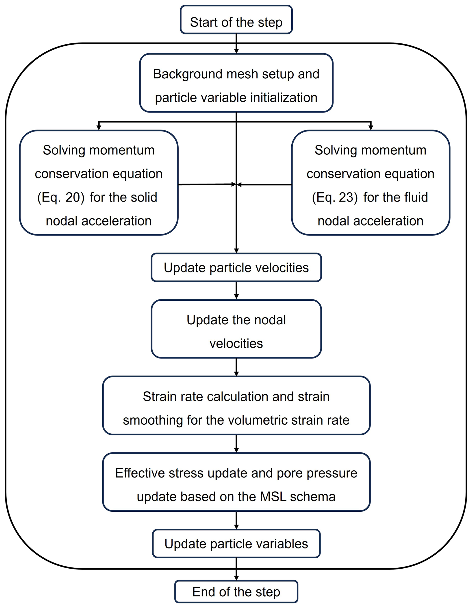
Figure 3 Numerical implementation procedure of the proposed stabilized two-phase MPM formulation.

The coefficient can be further expressed as

$$\begin{array}{}\text{(32)}& a=-{\mathit{H}}^{-\mathrm{1}}\underset{\mathrm{\Omega }}{\int }Q{\displaystyle \frac{K_{\mathrm{w}}}{n}}\left[\right(\mathrm{1}-n)\mathrm{\nabla }\cdot {\mathit{v}}_{\mathrm{s}}+n\mathrm{\nabla }\cdot {\mathit{v}}_{\mathrm{s}}]\mathrm{d}\mathrm{\Omega },\end{array}$$

where $\mathit{H}={\int }_{\mathrm{\Omega }}Q{Q}^{\mathrm{T}}\mathrm{d}\mathrm{\Omega }$. In order to solve the coefficient vector, the node-based method (Mast et al., 2012) is used due to its simplicity and efficiency. Using the node-based method, the node coefficient vector is written as

$$\begin{array}{}\text{(33)}& {\mathit{a}}_I=-{\mathit{H}}_I^{-\mathrm{1}}\sum _{p=\mathrm{1}}^{n_{\mathrm{p}}}{N}_{Ip}{Q}_p{\displaystyle \frac{K_{\mathrm{f}}}{n}}\left[\right(\mathrm{1}-n)\mathrm{\nabla }\cdot {\mathit{v}}_{\mathrm{s}}+n\mathrm{\nabla }\cdot {\mathit{v}}_{\mathrm{s}}]V_p,\end{array}$$

where ${\mathit{H}}_I=\sum _{p=\mathrm{1}}^{n_{\mathrm{p}}}{Q}_p{Q}_p^{\mathrm{T}}{N}_{Ip}{V}_p$. After solving the coefficient vector for each node, the changing rate of pore pressure can be written as

$$\begin{array}{}\text{(34)}& {\dot{p}}_{\mathrm{f}p}=Q_p^{\mathrm{T}}\sum _{I=\mathrm{1}}^{n_{\mathrm{g}}}{a}_I{N}_{Ip},\end{array}$$

where $\sum _{I=\mathrm{1}}^{n_{\mathrm{g}}}{a}_I{N}_{Ip}$ is the node value interpolated to the particle.

3.3 Numerical algorithm

In the proposed formulation, each time step is solved explicitly according to the following sequence of sub-steps (see Fig. 3):

1. All the variables associated with each material point are initialized first (initial position, stress, pore pressure, etc.).

2. The variables of material points are interpolated to the nodes of the background mesh using the shape function calculated based on particle locations with respect to the background mesh nodes.

3. Combined with the correct boundary conditions, the accelerations of each phase on the background mesh node are obtained based on Eqs. (20) and (23).

4. The velocity of all material points is updated for both phases using the FLIP scheme (Hammerquist and Nairn, 2017).

5. The nodal velocities for both phases are updated by interpolating velocities back from the material points.

6. Strain rate increments of solid and fluid phase on particles are calculated, and the cell-based strain smoothing technique expressed in Eq. (26) is applied to smooth the volumetric strain rate.

7. The effective stress is updated based on its constitutive model, and the pore pressure is updated based on the multi-field variational principle.

8. The state variables at particles are updated, such as particle volume, porosity, and position.

9. The background mesh for the next step is reset, and all the updated information is stored in material points.

4 Numerical examples

In this section, four numerical examples are conducted to demonstrate the performance of the proposed MPM formulation. Firstly, a one-dimensional consolidation under both small and large conditions is simulated. Subsequently, the two-dimensional consolidation under localized loading and cyclic loading is performed to show its efficacy under external loading. Then, the self-wight consolidation is analyzed to illustrate its capability in simulating undrained and drained conditions and the large-deformation situation.

4.1 One-dimensional consolidation

The one-dimensional consolidation problem has frequently been studied to verify and assess numerical methods, as it allows a direct comparison with analytical solutions. Here, both small- and large-deformation conditions are conducted, and the numerical results are compared with their corresponding analytical solutions.

4.1.1 Small deformation

As shown in Fig. 4, a saturated soil column with a width of 0.1 m and a length of 1.0 m is considered for the simulation. An isotropic linear elastic constitutive model is employed, with parameters detailed in Table 1. The background mesh consists of cells sized 0.05 m × 0.05 m, with 4 material points in each mesh element, resulting in a total of 160 material points. A normal impermeable roller boundary is applied to the lateral surfaces, while the bottom is fully fixed and impermeable. The top surface of the column is permeable, allowing fluid to flow out through it. The initial conditions include an excess pore pressure p₀ = 10 kPa and zero effective stress. Not considering gravity, the consolidation process begins by applying a 10 kPa traction to the top material point layer and keeping it constant during the calculation. The time step is set to be 1.0 × 10⁻⁵ s with a total simulation time of 2.0 s.

Figure 4 Schematic of the one-dimensional consolidation.

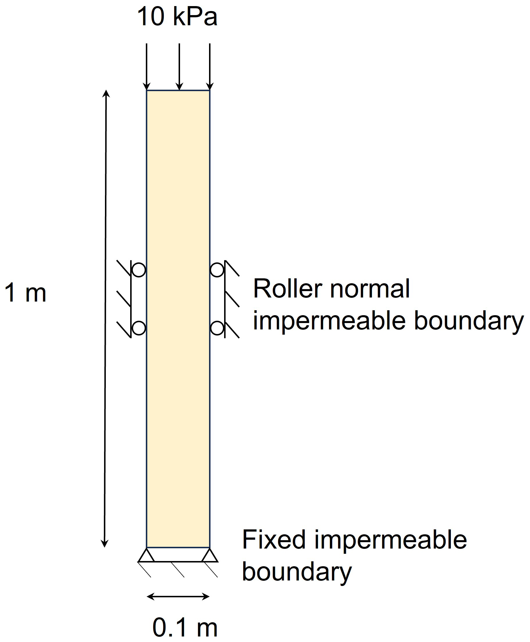
Table 1 Material parameters for the one-dimensional consolidation.

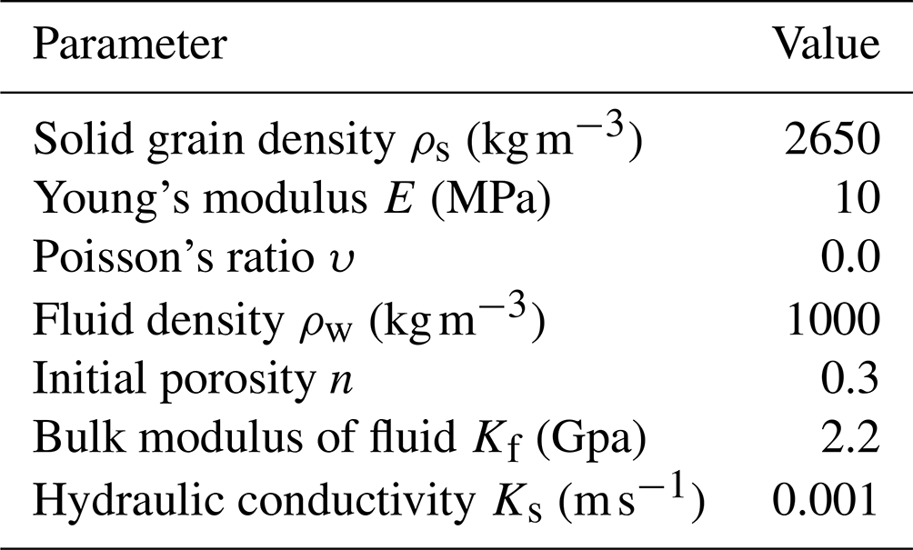
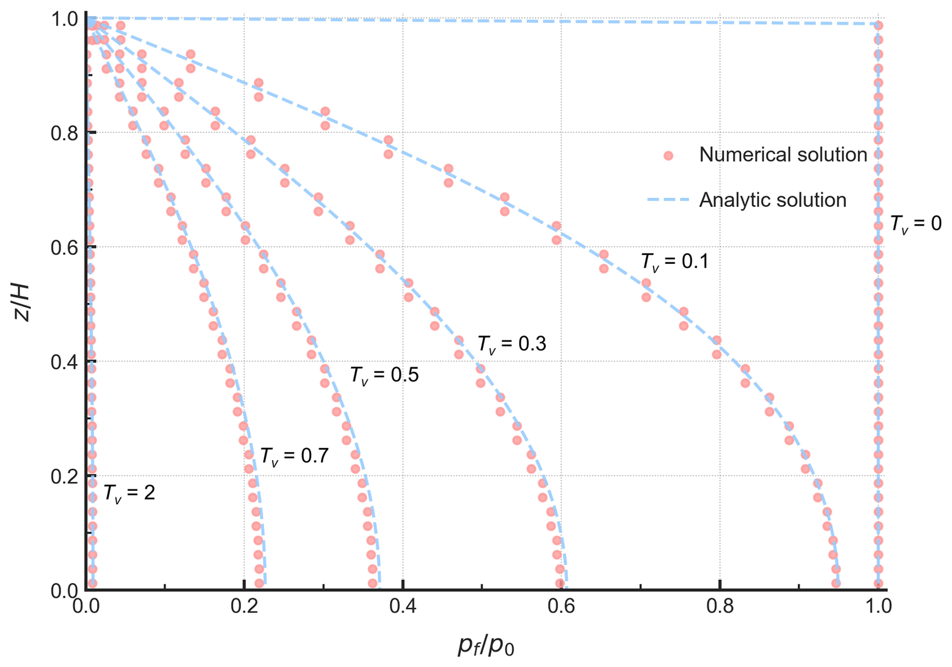
Figure 5 Comparison of pore pressure profiles from the proposed formulation with Terzaghi's solution.

Under such a constant loading, the deformation of the column is very small and Terzaghi's one-dimensional consolidation theory is applicable. Figure 5 presents a comparison of the normalized pore pressure distribution at different time factors between the numerical solution and the analytical solution (the time factor $T_{\mathrm{v}}=C_{\mathrm{v}}t/H^{\mathrm{2}}$, where C_v is the coefficient of consolidation and H is the drainage path length). Initially, the pore pressure equals the external load, with the fluid phase undertaking the external loading. Since the external loading is constant, the pore fluid is gradually discharged from the top surface and the pore pressure begins to dissipate progressively from the top. The numerical results show excellent agreement with the analytical solutions, effectively capturing the dissipation process of the excess pore pressure during consolidation. Additionally, the comparison of the average consolidation degree (defined by strain) is presented in Fig. 6, indicating that the numerical results accurately replicate the deformation process as the analytical solution shows.

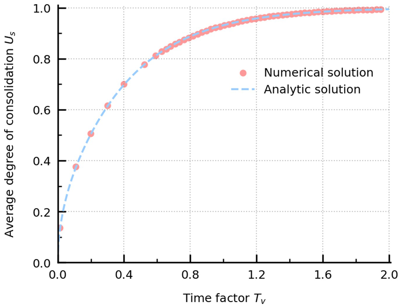
Figure 6 Comparison of the average degree of consolidation from the proposed formulation with Terzaghi's solution.

4.1.2 Large deformation

For the large-deformation condition, the same geometry and discretization as in the small-deformation case are used. However, a larger top traction (0.2 MPa) is applied, a softer material (E = 1 MPa) is considered, and the hydraulic conductivity K_s is adjusted to be 0.0001 m s⁻¹. Accordingly, the pore pressure is initialized at 0.2 MPa, ensuring that the loading is initially fully carried by the fluid phase. Similarly to the small-deformation case, the pore pressure will gradually dissipate after applying the constant loading, but now this process will generate considerable vertical deformation. The decrease in the column length is not negligible; therefore the small-strain Terzaghi's theory is no longer applicable. Based on the large-deformation analytical solution (Xie and Leo, 2004), the evolution of pore pressure, top settlement, and the average degree of consolidation (defined by strain) can be expressed as

$$\begin{array}{}\text{(35)}& {\displaystyle }\begin{array}{rl}{p}_{\mathrm{f}}(z,t)=& {\displaystyle \frac{\mathrm{1}}{m_{\text{vl}}}}\ln [\mathrm{1}+(e^{m_{\text{vl}}{p}_{\mathrm{a}}}-\mathrm{1})\sum _{m=\mathrm{1}}^{\mathrm{\infty }}{\displaystyle \frac{\mathrm{2}}{M}}\sin \left({\displaystyle \frac{Mz}{H}}\right)\\ & \times e^{-M^{\mathrm{2}}{T}_{\mathrm{v}}}],\end{array}\text{(36)}& {\displaystyle }{S}_{\mathrm{t}}=H_{\mathrm{0}}(\mathrm{1}-e^{-m_{\text{vl}}{p}_{\mathrm{a}}})\left(\mathrm{1}-\sum _{m=\mathrm{1}}^{\mathrm{\infty }}{\displaystyle \frac{\mathrm{2}}{M^{\mathrm{2}}}}{e}^{-M^{\mathrm{2}}{T}_{\mathrm{v}}}\right),\text{(37)}& {\displaystyle }{U}_{\mathrm{s}}=\mathrm{1}-\sum _{m=\mathrm{0}}^{\mathrm{\infty }}{\displaystyle \frac{\mathrm{2}}{M^{\mathrm{2}}}}{e}^{-M^{\mathrm{2}}{T}_{\mathrm{v}}},\end{array}$$

where $m_{\text{vl}}=\mathrm{1}/E$ is the one-dimensional compressibility, p_a is applied external load, H₀ is the initial depth of the column, and z is the distance to the top surface. With the same time step, the total simulation time is 300.0 s.

Figure 7 shows the numerical solution of pore pressure evolution along the column height against the results from the analytic solution at different average degrees of consolidation. In the small-deformation case, the consolidation coefficient C_v is equal to 1, while, for the large-deformation case, the consolidation coefficient C_v is very small, so the consolidation is a long process. Hence, the pore pressure dissipation here is much slower than in the small-deformation case. The comparison shows that the numerical results are consistent with the analytic solutions and accurately depict this large-deformation consolidation process. The cell average method used in the strain smoothing method will give the same volumetric strain rate for the particles in the same mesh cell, resulting in the same pore pressure distribution in each mesh cell, but the overall trend of this large consolidation process can still be captured. Figure 8 shows the evolution of the settlement at the top surface. The numerical result (final top settlement: 0.1815 m) is very close to the analytic result (final top settlement: 0.1802 m). The comparison demonstrates the validation and applicability of the proposed formulation in this two-phase large-deformation process.

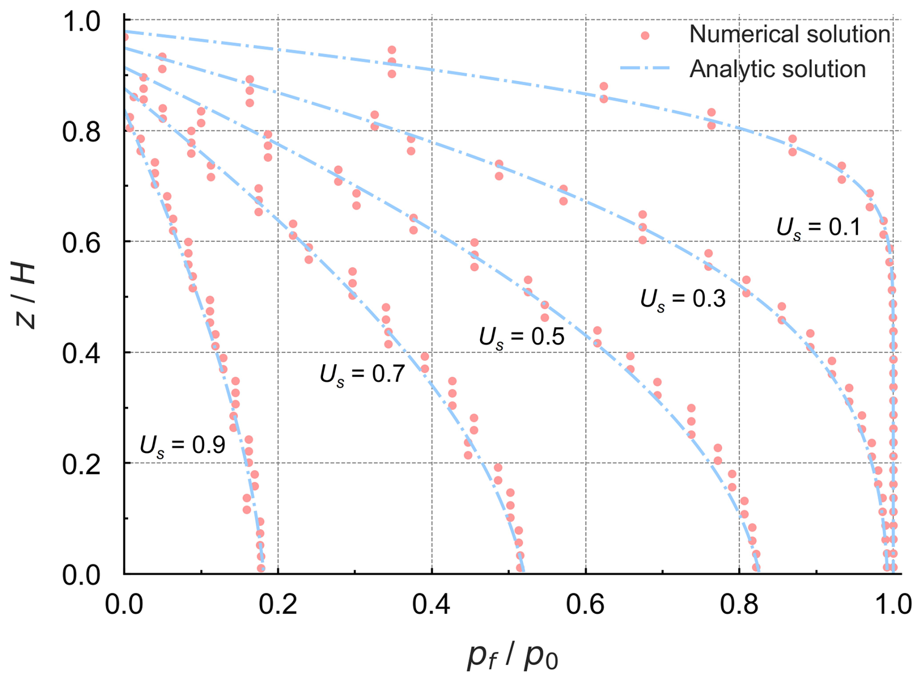
Figure 7 Comparison of pore pressure profiles from the proposed formulation with analytic solution.

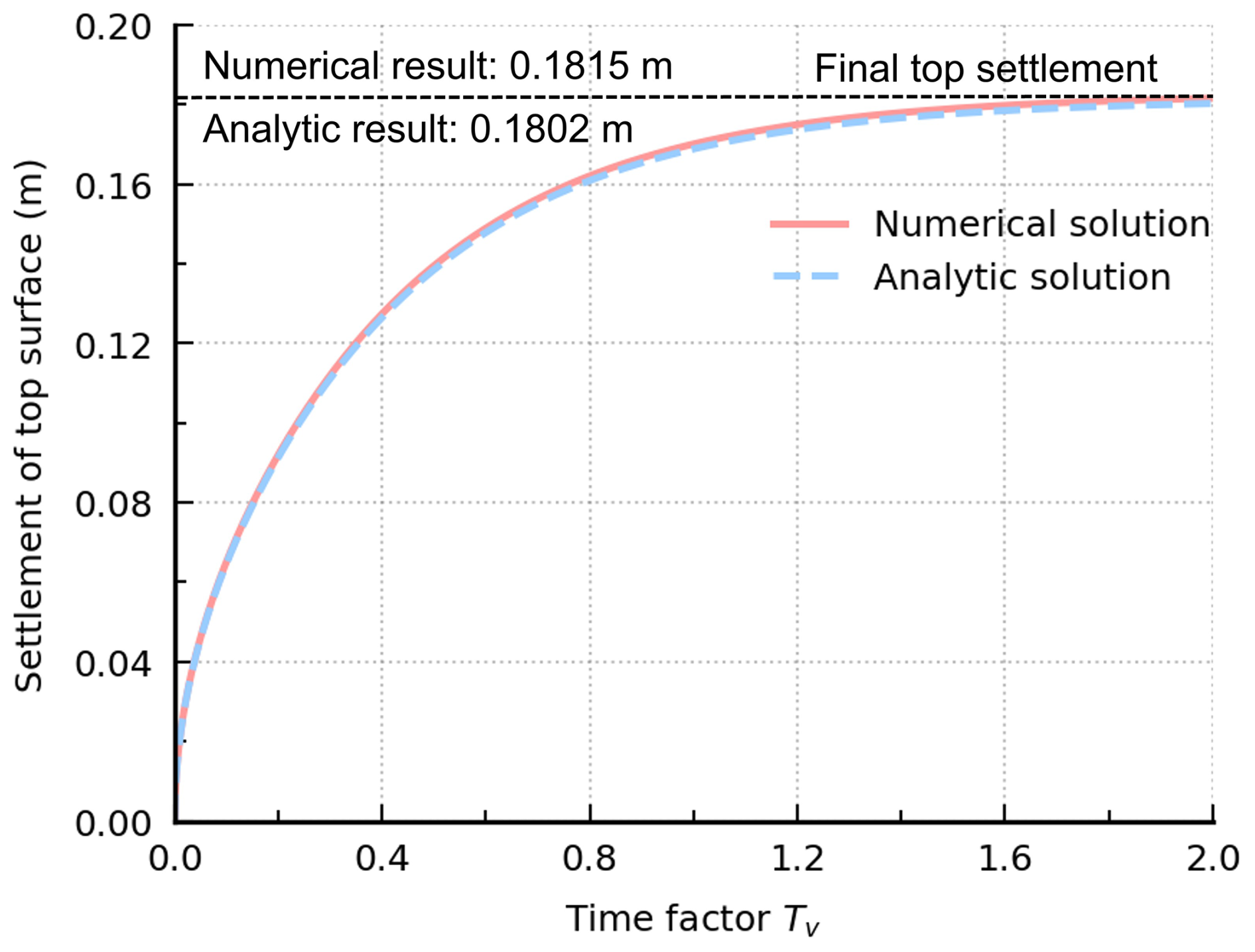
Figure 8 Comparison of the top settlement from the proposed formulation with analytic solution.

4.2 Two-dimensional consolidation under localized loading

In this section, a two-dimensional elastic consolidation under a localized loading is simulated, with the geometry and boundary conditions illustrated in Fig. 9. Due to the symmetry of the problem, only half of the domain is modeled. The saturated material domain possesses a dimension of 10.0 m × 10.0 m, while the background mesh consists of cell elements sized 0.05 m × 0.05 m, with four material points in each cell element, resulting in 1600 particles. A normal impermeable roller boundary is applied to the lateral surfaces and the bottom, while the top surface is permeable and unconstrained. Initially, a constant local loading of 20.0 kPa, spanning a width of 0.3 m, is applied on the left side of the top surface. Without considering gravity, the initial stress and pore pressure are set to be 0. The isotropic linear elastic constitutive model is used, and the material parameters are provided in Table 2. The time step of the simulation is 2.0 × 10⁻⁴ s, and the total simulation time is 0.1 s. The same simulation was conducted in previous studies by a semi-implicit MPM scheme (Yuan et al., 2023; Kularathna et al., 2021).

Figure 9 Model setup for the two-dimensional consolidation.

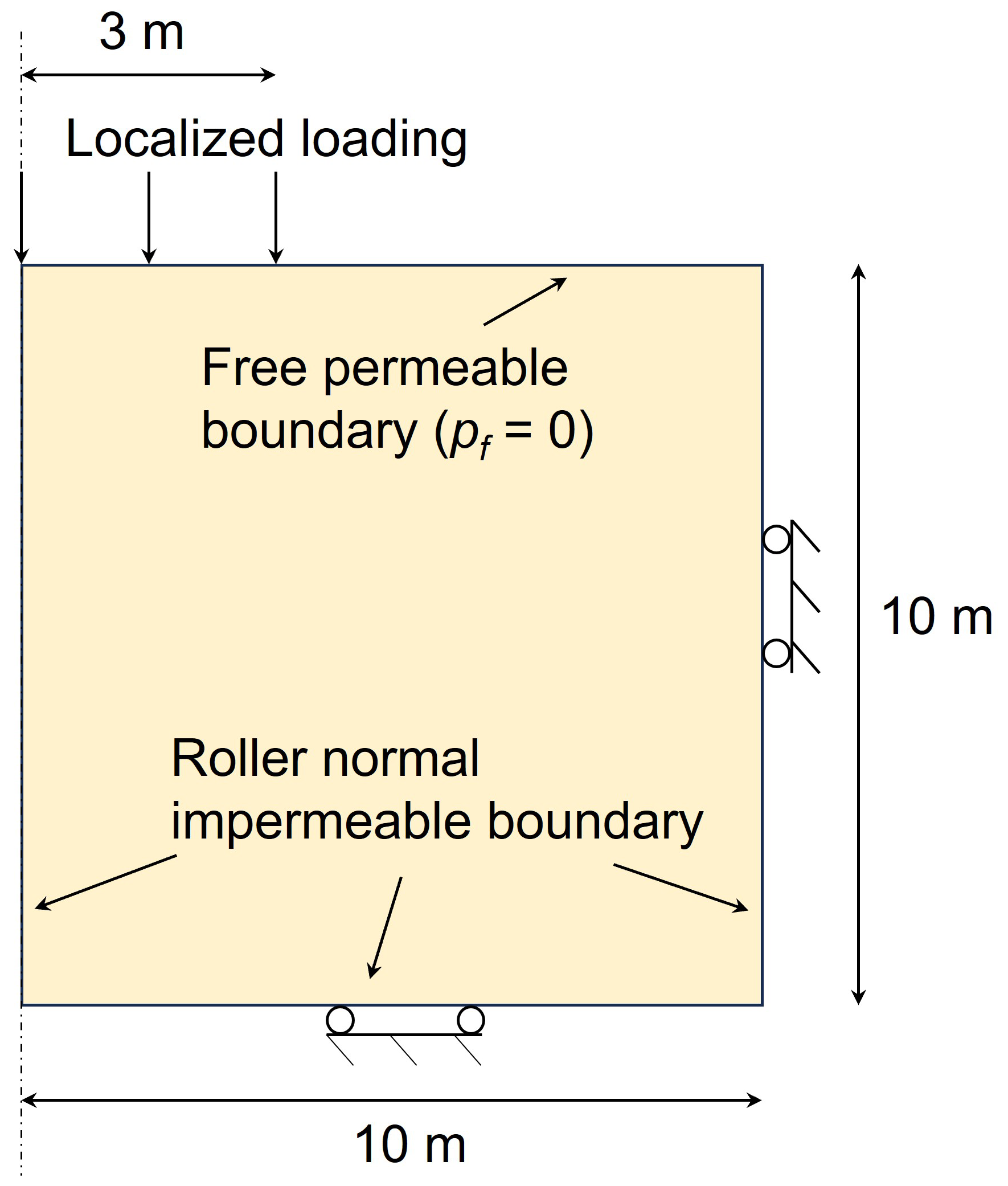
Table 2 Material parameters for the two-dimensional consolidation.

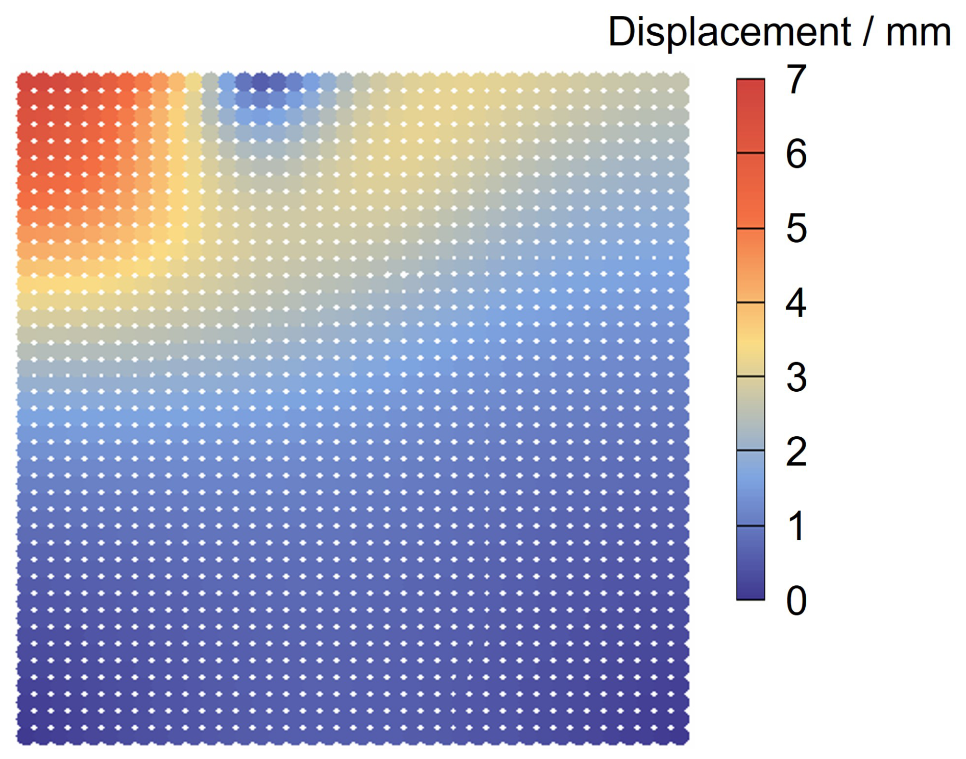
Figure 10 illustrates the distribution of pore pressure at time t = 0.1 s, comparing the results obtained with and without stabilized techniques. In Fig. 10b, a spurious pore pressure field with a checkerboard distribution is observed. In contrast, the result with stabilized techniques shows a smooth excess pore pressure field caused by the external loading (Fig. 10a). It demonstrates that the stabilized techniques can mitigate pore pressure oscillation well in the two-phase MPM formulation, offering a stable pressure distribution. The displacement distribution at t = 0.1 s is shown in Fig. 11. Consistent with the applied local loading, the displacement mainly occurs in the local loading region, indicating that the local loading is undertaken by the upper-left corner area. The maximum displacement (6.737 mm) occurs at the top-left corner, which is consistent with the results from the semi-implicit MPM formulation (Yuan et al., 2023). Similar results are also obtained using the semi-implicit MPM with artificial compressibility stabilization and the fractional step method (Yuan et al., 2023; Kularathna et al., 2021). The stabilized techniques employed here can yield equivalent results that are free of stress oscillations while accurately preserving the mechanical behavior.

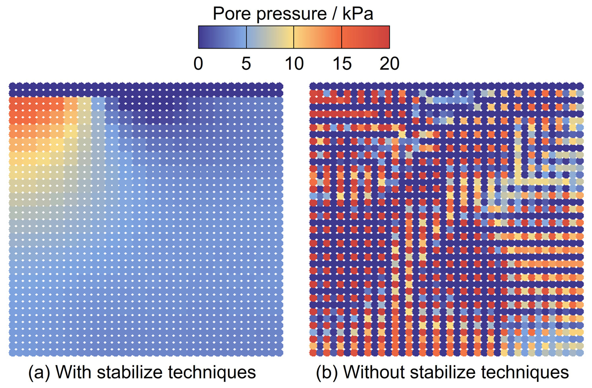
Figure 10 Pore pressure distribution with stabilized techniques and without stabilized techniques at t = 0.1 s.

Figure 11 Distribution of displacement field at time t = 0.1 s.

Figure 12 Schematic of the cyclic loading test.

4.3 Cyclic loading test

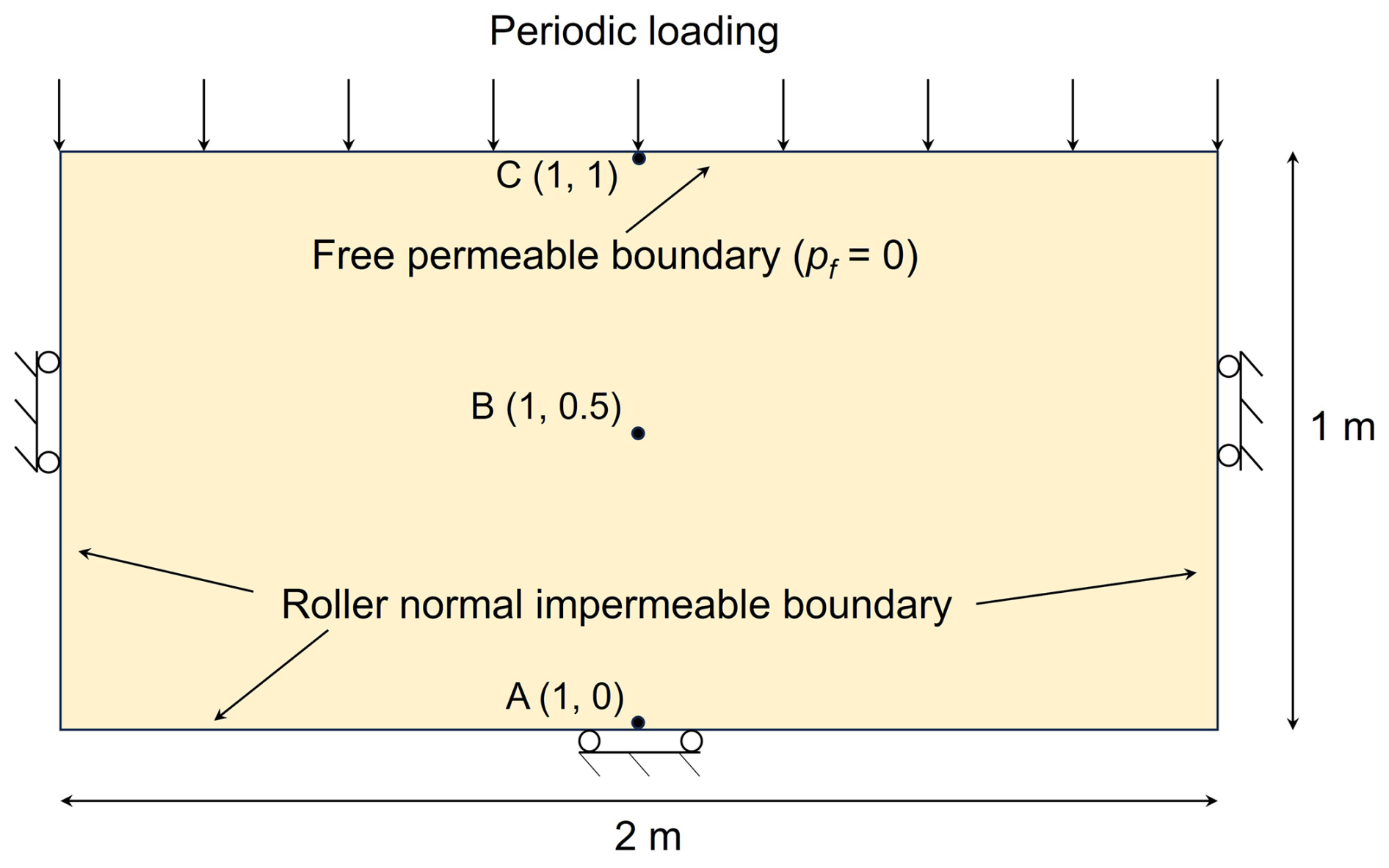
Inspirited by the lateral cyclic loading test (Liang et al., 2023), we conduct a vertical cyclic loading test of a saturated granular material. The model setup is shown in Fig. 12, where the saturated material is placed in a rigid box and subjected to a vertical cyclic loading. The material domain measures 2 m in width and 1 m in height and is discretized by a quadrilateral element with a size of 0.05 m × 0.05 m, and there are 4 particles in each element, giving 3200 particles. Both the bottom and laterals are normal impermeable and supported by rollers, and the top is unconstrained and permeable. To apply a cyclic loading, the top surface is prescribed by a sinusoidal function periodic load of 40sin 5πt kPa. Table 3 lists the material parameters used for the isotropic linear elastic constitutive model. Before the cyclic stimulation, an equilibrium condition is achieved by a linear gravity loading from 0 to 9.81 m s⁻² within $\mathrm{0}\le t\le$ 0.1 s; then, the gravity remains constant. To monitor the cyclic loading response, three monitoring points located at the bottle, middle, and top of the material domain (A, B, C) are selected (as shown in Fig. 12). The time step is set to be 1.0 × 10⁻⁵ s, and the simulation is terminated at 2.1 s.

Table 3 Material parameters for the cyclic loading test.

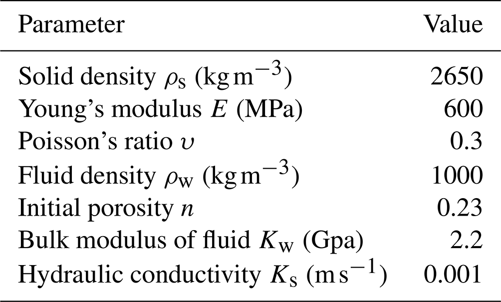
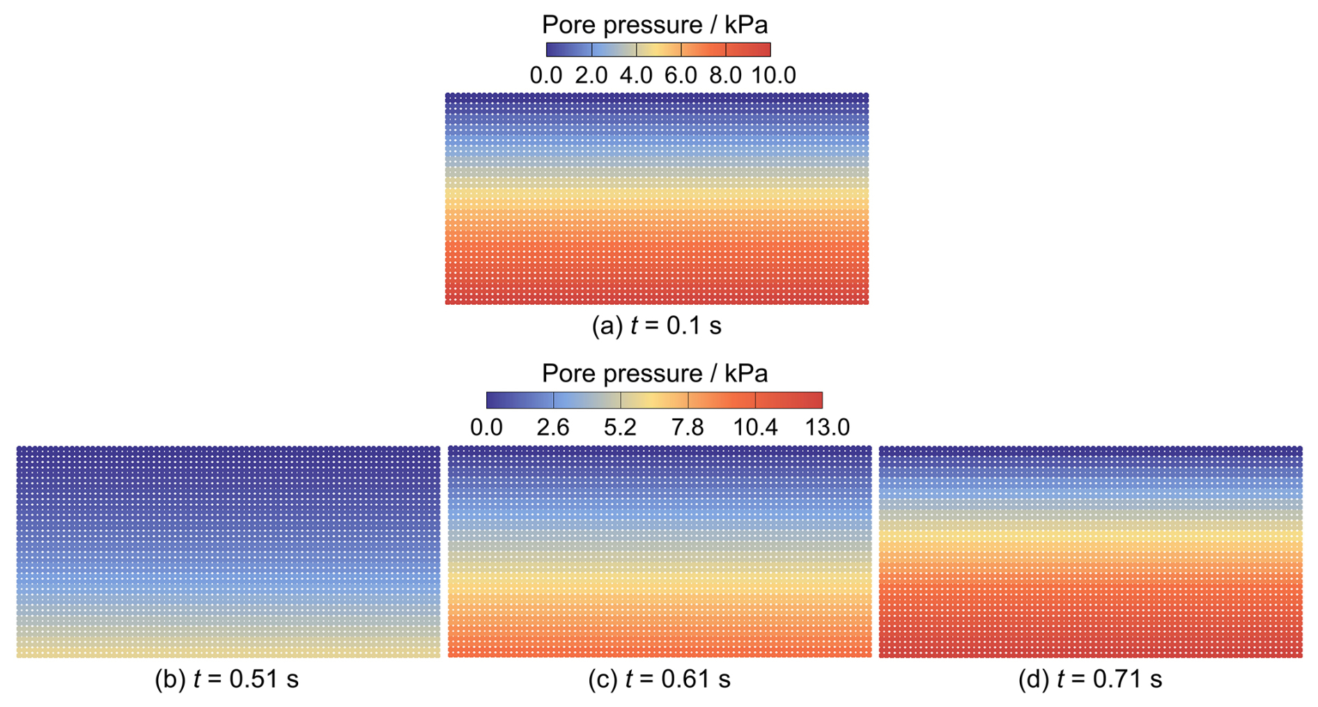
Figure 13 Distribution of pore pressure at t = 0.1 s (hydrostatic pressure), t = 0.51 s, t = 0.61 s, and t = 0.71 s.

Figure 13 shows the generated pore pressure at four different time instants. After the application of linear gravity loading, an equilibrium condition is achieved and a hydrostatic pressure field is generated (Fig. 13a). Subsequently, a vertical cyclic loading is applied to the surface. When the material domain is subjected to compressive loading, the pore pressure field increases, whereas, under tensile loading, the pore pressure field decreases correspondingly. This vertical cyclic shaking induces an apparent periodic buildup and dissipation of excess pore pressure in the material domain. In Fig. 13b, a clear pore pressure decrease due to tensile loading at t = 0.51 s can be seen. As the tensile loading gradually decreases and shifts into compressive loading, the pore pressure will gradually raise up. As a result, the pore pressure field returns to the hydrostatic state at t = 0.61 s (Fig. 13c). Subsequently, the compressive loading leads to a further increase in pore pressure. As depicted in Fig. 13d, a significant excess pore pressure field is regenerated. Therefore, the pore pressure in the material domain exhibits periodic variations in response to the cyclic loading.

Figure 14 Evolution of pore pressure and displacement at selected points.

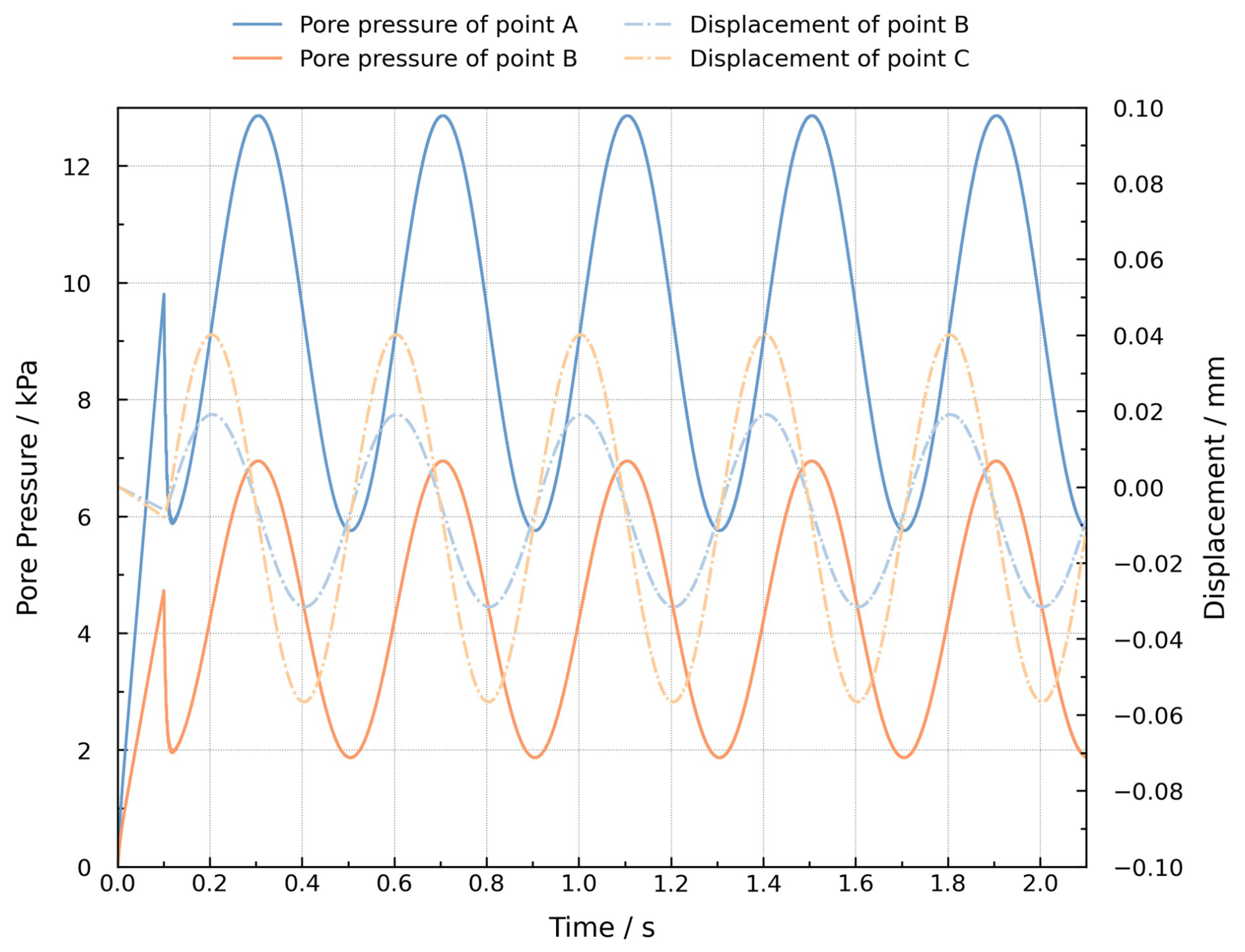
To further present the cyclic dynamic response under the applied cyclic loading, the evolution of pore pressure and displacement at the selected monitoring points is presented in Fig. 14. The time history of pore pressure and displacement over time demonstrates this cyclic loading response more quantitatively and vividly. The linear gravity loading ends at t = 0.1 s, during which the displacement remains very small. After that, the vertical loading will induce a relatively large displacement. Under the sinusoidal periodic loading, the vertical displacement of point B and C exhibits a sinusoidal variation and the pore pressure at point A and B also changes accordingly. These cyclic responses can be well captured by the proposed stabilized MPM formulation.

4.4 Self-weight consolidation

The large-deformation consolidation of an elastic slumping block under gravity loading is presented in this section (Fig. 15), which is related to the settlement of a very soft soil and has been simulated in previous studies (Zheng et al., 2021, 2022; Sang et al., 2024; Wang et al., 2023a). The simulation focuses on the right half of a symmetric domain with dimensions of 4 m width and 2 m height. The material domain is discretized using quadrilateral elements of size 0.125 m × 0.125 m and 4 particles in each element, giving 1024 particles in total. No external load is applied, making the consolidation process solely driven by the initial gravitational force at the start of the simulation. The gravity linearly increases from 0 to 9.81 m s⁻² within $\mathrm{0}\le t\le$ 0.1 s and then remains constant. Both the top and right boundaries are unconstrained and freely draining, while the left and bottom boundaries are normally impermeable and supported by rollers. The gravity will give rise to pore pressure buildup, while the deformation will lead to the dissipation of pore pressure over time, and two points (P₁, P₂) at the bottle and middle are selected to evaluate the consolidation process (as shown in Fig. 15). An isotropic linear elastic constitutive model is used, and the parameters are listed in Table 4. The total simulation time is 0.5, and the simulation is performed with a time step equal to 1.0 × 10⁻⁶ s.

Figure 15 Schematic of the self-weight consolidation.

Table 4 Material parameters for the self-weight consolidation.

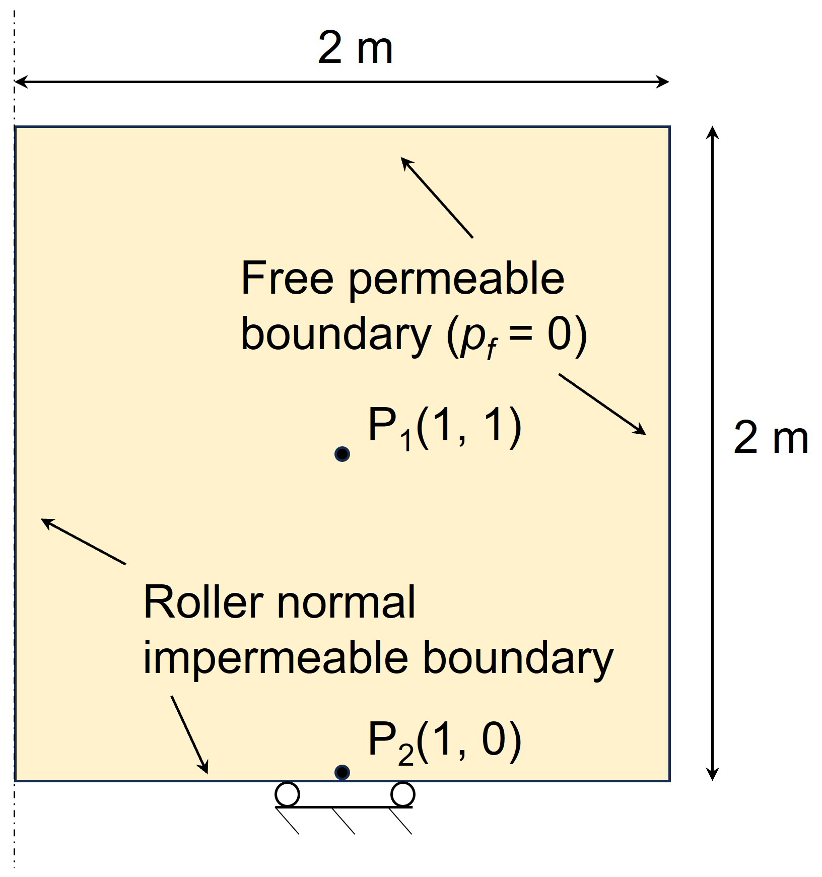
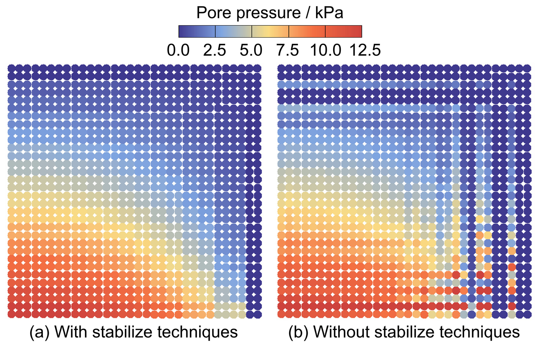
Figure 16 Pore pressure distribution at t = 0.05 s obtained with stabilized techniques and without stabilized techniques.

Figure 17 Pore pressure distribution at different times.

Figure 18 Deviatoric stress distribution at different times.

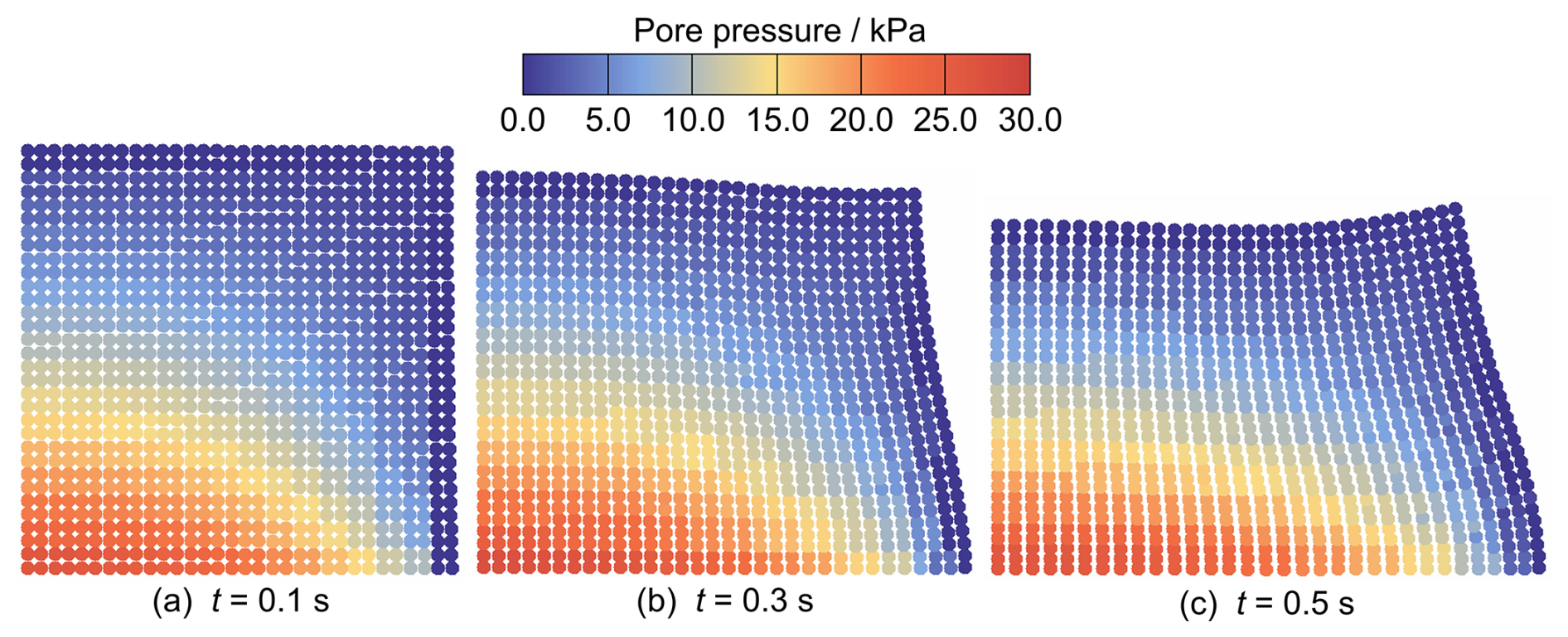
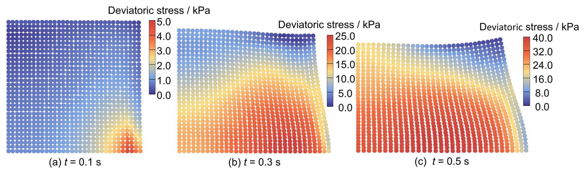
Initially, due to the relatively quick application of gravity loading, the pore fluid cannot be rapidly discharged, and the loading process is carried out under approximately undrained conditions. Therefore, the applied gravity loading will induce excess pore pressure at the beginning. Figure 16 shows pore pressure fields after gravity loading (t = 0.05 s) with stabilized techniques and without stabilized techniques. It can be seen that the result without stabilized techniques suffers from pore pressure oscillations. The stabilized result, in contrast, eliminates spurious oscillations effectively under stringent undrained conditions. Moreover, the distribution of pore pressure and deviatoric stress at three different times (0.1, 0.3, and 0.5 s) is illustrated in Figs. 17 and 18, respectively. Upon the application of linear gravity loading, a pore pressure field develops, gradually decreasing from the bottom-left corner upwards, as shown at t = 0.1 s (Fig. 17a). At this stage, the deformation is not large, with a localized region of deviatoric stress distribution observed near the bottom-right corner (Fig. 18a). Subsequently, gravity continues to generate pore pressure, and the deviatoric stress gradually increases as deformation progresses. As deformation develops under gravity, the pore pressure first reaches the maximum value and then dissipates because of the deformation and drainage at the boundary. This process can be observed in Figs. 17b, 18b and Figs. 17c, 18c. Both pore pressure and deviatoric stress changed continuously along the large-deformation process. The absence of checkerboard oscillations shows the stability of the proposed stabilized formulation in capturing the mechanical behavior of the slumping block during the consolidation process.

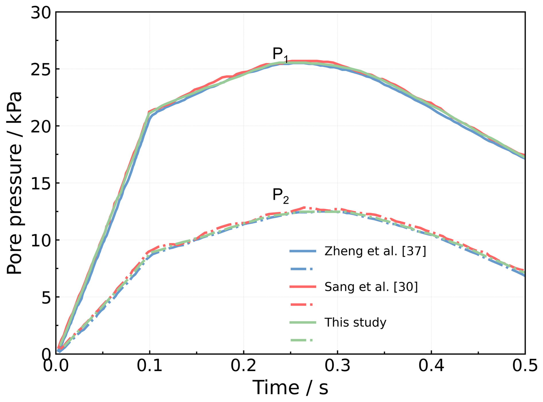
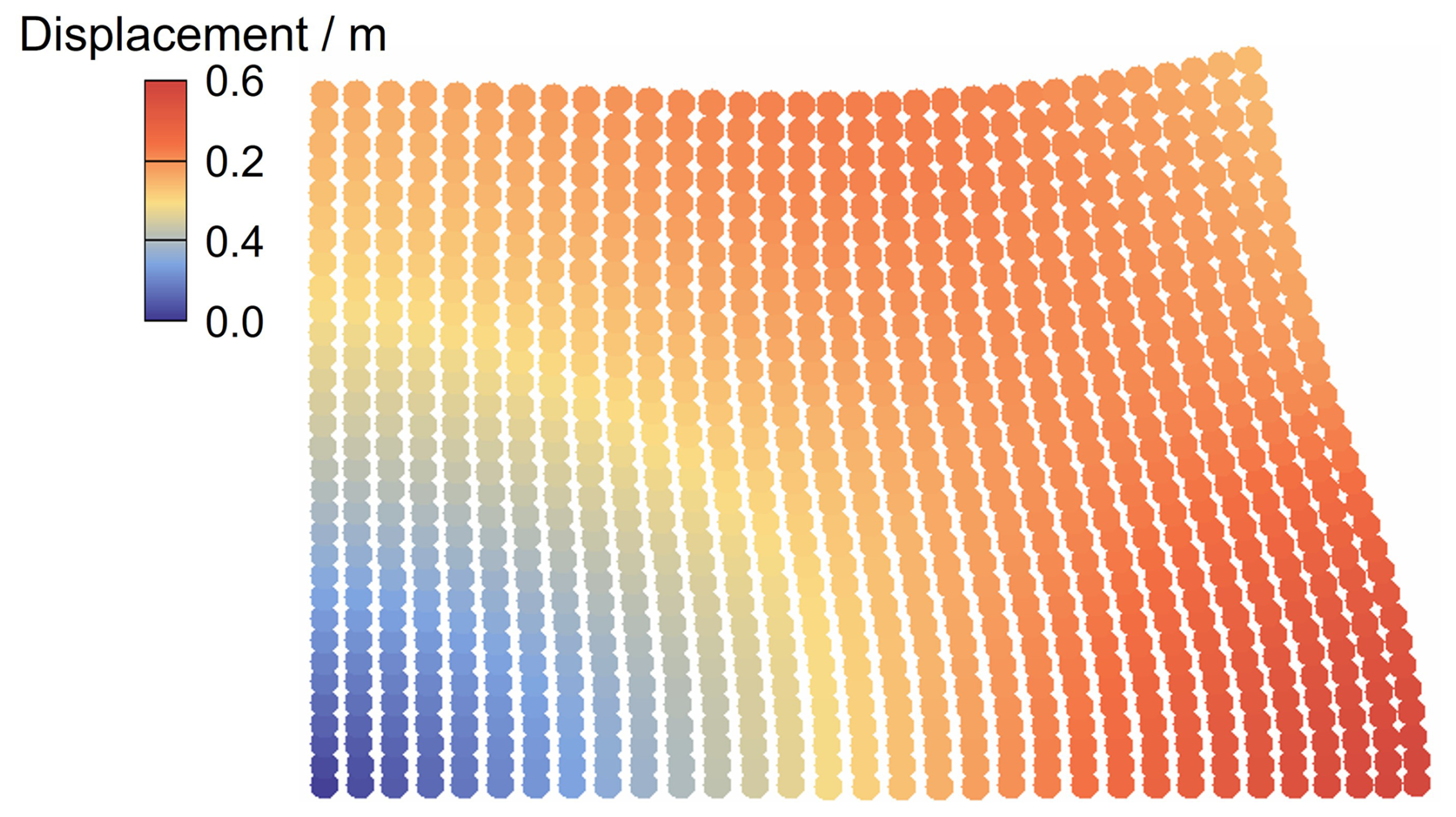
To further verify the accuracy of the results, the time evolution of the pore pressure at two points (P₁, P₂ in Fig. 15) is shown in Fig. 19, and the results are compared with those of Zheng et al. (2022) using implicit stabilized MPM formulation and Sang et al. (2024) using implicit coupled MPM formulation. During the linear gravity loading, pore pressure increases linearly, followed by non-monotonic dissipation due to the Mandel–Cryer effect. The curves obtained using the proposed stabilized formulation agree well with those of Zheng et al. (2022) and Sang et al. (2024), and the final displacement field (Fig. 20) closely matches the results reported in previous studies (Wang et al., 2023a; Yuan et al., 2023).

Figure 19 Pore pressure evolution at two selected points.

Figure 20 Displacement distribution at 0.5 s.

5 Discussion and conclusions

For the hydromechanical coupling problems in solid–fluid porous media, this study presents an explicit stabilized two-phase material point method by incorporating the strain smoothing method and the multi-field variational principle in the single-point two-phase MPM scheme. The proposed model effectively mitigates pore pressure oscillation and maintains numerical stability.

The proposed two-phase MPM was initially validated through a one-dimensional consolidation problem under both small- and large-deformation cases, with the numerical results showing strong agreement with analytical solutions. It was further assessed through two-dimensional consolidation under localized loading and cyclic loading, demonstrating the formulation's ability in accurately capturing the dynamic response of saturated porous media under external loads. Finally, the self-weight consolidation was analyzed to showcase its efficacy in simulating both undrained and drained conditions and in handling large-deformation problems. The results aligned closely with analytical solutions and outcomes from other approaches. In particular, the pore pressure instabilities were greatly mitigated by the stabilized techniques, as clearly validated by the numerical results in terms of pore pressure.

With its effective and easy-to-implement stabilized techniques, the proposed two-phase MPM formulation is well suited for analyzing a wide range of hydromechanical processes under various undrained, drained, and loading conditions. It offers an effective and reliable approach for simulating both static and dynamic processes in solid–fluid porous media. While the current work is limited to the linear elastic behavior of the solid phase, future efforts will focus on the practice and application involving more complex large-deformation problems and advanced constitutive models.