Comparing an idealized deterministic–stochastic model (SUP model, version 1) of the tide- and wind-driven sea surface currents in the Gulf of Trieste to high-frequency radar observations

In the Gulf of Trieste, the sea surface currents were observed by high-frequency radar for almost 2 years (2021–2022) at a temporal resolution of 30 min. We developed a hierarchy of idealized models to simulate the observed sea surface currents, combining a deterministic and a stochastic approach, in order to reproduce the externally forced motion and the internal variability, which is characterized by fat-tailed statistics. The deterministic signal includes tidal and Ekman forcing and resolves the slowly varying part of the flow, while the stochastic signal represents the fast-varying small-scale dynamics, characterized by Gaussian or fat-tailed statistics, depending on the statistic used. This is done using Langevin equations and modified Langevin equations with a gamma-distributed variance parameter. The models were adapted to resolve the dynamics under nine tidal and wind forcing protocols in order to best fit the observed forced motion and internal variability probability density function (PDF). The stochastic signal requires 2 stochastic degrees of freedom when the average tidal forcing is adopted, while it needs $\mathrm{1}/\mathrm{2}$ stochastic degree of freedom when the complete tidal forcing is used. Despite its idealization, the deterministic–stochastic model with stochastic fat-tailed statistics captures the essential dynamics and permits mimicking the observed PDF. Moreover, a fluctuation response relation is valid when the stochastic signal is perturbed, showing that the response to an external perturbation can be obtained by considering the fluctuations of the unperturbed system.

1 Introduction

The Gulf of Trieste is a shallow, semi-enclosed basin in the northern Adriatic Sea (Mediterranean Sea, Fig. 1). Its surface circulation is influenced by the broader Adriatic cyclonic (anti-clockwise) circulation and the basin's thermohaline stratification and circulation (Cosoli et al., 2012; Querin et al., 2021). Due to its shallowness and small scale (horizontal length scale of around 20 km and depth of around 25 m), its current dynamics highly depend on two external forcings: the wind forcing and the Isonzo/Soc̆a river freshwater input (Querin et al., 2006; Cosoli et al., 2012, 2013; Querin et al., 2021).

The Bora and the Sirocco are the main strong wind patterns affecting the dynamics in the Gulf of Trieste. The Bora is an east-north-easterly katabatic wind, bringing cold and dry air from the continent over the sea (Poulain and Raicich, 2001). Its strength is heavily influenced by the local topography, making it particularly powerful over the Gulf of Trieste, where it can reach gusts up to 180 km h⁻¹. When it blows, surface water is pushed out of the gulf towards the Adriatic basin, and a compensating bottom counter-current flows in, causing upwelling on the coastal side (Malačič et al., 2001; Querin et al., 2006; Reyes Suárez et al., 2022). The Sirocco is a moist, warm and relatively mild southerly wind, channelled by the Adriatic coastal mountains. It causes sea level rise in the northern Adriatic, leading to a strong southward return flow when the wind diminishes (Cosoli et al., 2012).

In recent years, the Gulf of Trieste has benefitted from an abundance of observational data, particularly high-frequency radar (HFR) sea surface currents. The amount of data will strongly increase in the near future. This large amount of data allowed for a statistical approach to characterize the data (Flora et al., 2023). In particular, the authors found the analytical probability density function (PDF) of the observed HFR sea surface velocity increments using a superstatistical (a superposition of statistics) analysis and the principle of maximum entropy. Superstatistical analysis (Beck et al., 2005) considers a system with a clear timescale separation: at a fast timescale, a Gaussian PDF is observed, of which the variance evolves slowly, on the long timescale. In the Gulf of Trieste, the fast timescale of around 2 h is consistent with the turbulence of the mixed-layer dynamics. The slow timescale of almost 2 d is consistent with the variability of the synoptic wind forcing, and the variance is distributed according to a gamma distribution with a shape parameter equal to 2. The Gaussian is the minimum entropy PDF with a finite variance, and the gamma distribution is the minimum entropy PDF for a positive variable, as is the variance, with a specified mean. The total PDF of the sea surface velocity increments is a fat-tailed PDF, which means that extreme events occur more often than in Gaussian statistics. The superstatistical analysis, however, is descriptive and has no predictive skills.

When modelling the turbulent ocean currents subject to a known wind forcing, there is part of the dynamics that can be described by a deterministic model and the unresolved turbulent processes that have to be described stochastically. This concept is reflected in stochastic differential equations (SDEs) and the corresponding Fokker-Planck equations. The former consider the evolution of many possible realizations, which allow construction of a time-evolving PDF, while the latter describe the deterministic evolution of the PDF. The use of SDEs in air–sea interaction was pioneered by Hasselmann (1976), who initiated a strand of scientific research on stochastic climate models. Taking into account the coupled ocean–atmosphere–cryosphere–land system, he divided it into a fast varying “weather” system and a slowly responding “climate” system, clearly separated by a fast and a slow timescale. In his modelization, the slow climate variables play the role of large particles interacting with an ensemble of smaller particles, i.e. the fast weather variables in the analogy, of the so-called Brownian motion problem. In this picture, the dispersion of the climate variables is inferred from the statistics of the weather variables with which they interact.

Brownian motion was first analytically described by Einstein (1905) and Langevin (1908) (see Einstein, 1956 and Lemons and Gythiel, 1997, respectively, for an English translation). Since that time, the SDE of the motion of a Brownian particle has been called the “Langevin equation”. The SDE approach, adopted also in this paper, has been widely used in the past decades in a variety of scientific fields: statistical mechanics (Baldovin et al., 2018), condensed matter physics (Silveira and Aarão Reis, 2012), marine biology and oceanography (Brillinger and Stewart, 2010), space weather science (Alberti et al., 2018), biophysics (Ham et al., 2022), and finance (Wand et al., 2024), to name a few. Regarding climate science, the Langevin equation has been widely used (Berglund and Gentz, 2002; Wirth, 2019; van den Berk et al., 2021), and great improvements have been achieved. Franzke et al. (2015) and Palmer (2019) show that including stochasticity into the parameterized representations of subgrid processes of physical climate systems has improved the skill of forecasts and reduced systematic model error. It is important to remark that the use of additive noise in linear SDE has limitations in terms of extreme event predictability, as it leads to Gaussian statistics. Adopting multiplicative noise or nonlinear damping, taking into account nonlinear interactions between resolved and unresolved modes of variability (Franzke et al., 2005; Wirth, 2018) leads to non-Gaussian statistics, increasing the fatness of the PDF tails of the modelled variables (Sura, 2013).

Modern concepts of non-equilibrium statistical mechanics have been applied to environmental fluid dynamics and to components of the climate system. Often, these considerations are limited to conceptual pertinence and tested on idealized models, such as the Lorenz models (Lorenz, 1996) and others, or on data from numerical models. In the present work, we apply a hierarchy of idealized models for the sea surface current observations from the Gulf of Trieste, starting with a deterministic modelization and then adding increasingly complex stochasticity. For solving these models, we rely on analytical calculations where possible and proceed with solutions of involved SDEs. This approach enables connecting observational data in a systematic way to the underlying principles of physics.

Our modelling approach is idealized and local: it considers one point in space, evolving in time, with wind shear and tidal deterministic forcing and a stochastic signal that mimics all the smaller unresolved scale dynamics. The aim of the modelization is to simulate the evolution of the forced motion and of the observed analytical PDF. It is based on the slow evolution of a short-timescale Gaussian and can be interpreted by an SDE. This enables us to understand what is the role of the stochasticity in the simulation of the Gulf of Trieste wind- and tide-driven circulation. The model is finally used to test the fluctuation response relation (FRR), described by Lacorata and Vulpiani (2007), that relates the system's reaction to external perturbations to spontaneous fluctuations of the unperturbed system. An evaluation of the forecasting of ocean currents based on the SDE predictability is also given.

In Sect. 2, the observed HFR sea surface data and the model forcing atmosphere data are presented. In Sect. 3, the modelization is explained with some FRR background and predictability evaluation methodology, while the computational results and their discussion are given in Sect. 4. The conclusions are reported in Sect. 5. In the Appendixes, the details and methods of the analytical calculations are shown.

2 The data

Two classes of time series are used: the observed sea surface horizontal HFR current data and the forecasted wind data for the Gulf of Trieste (northern Adriatic Sea, Fig. 1a). The data sets used are identical to those presented in Flora et al. (2023); they refer to a selected grid point in the Gulf of Trieste (point P and point WRF_P in Fig. 1b) and cover a time range of almost 2 years: from 1 January 2021 to 18 October 2022.

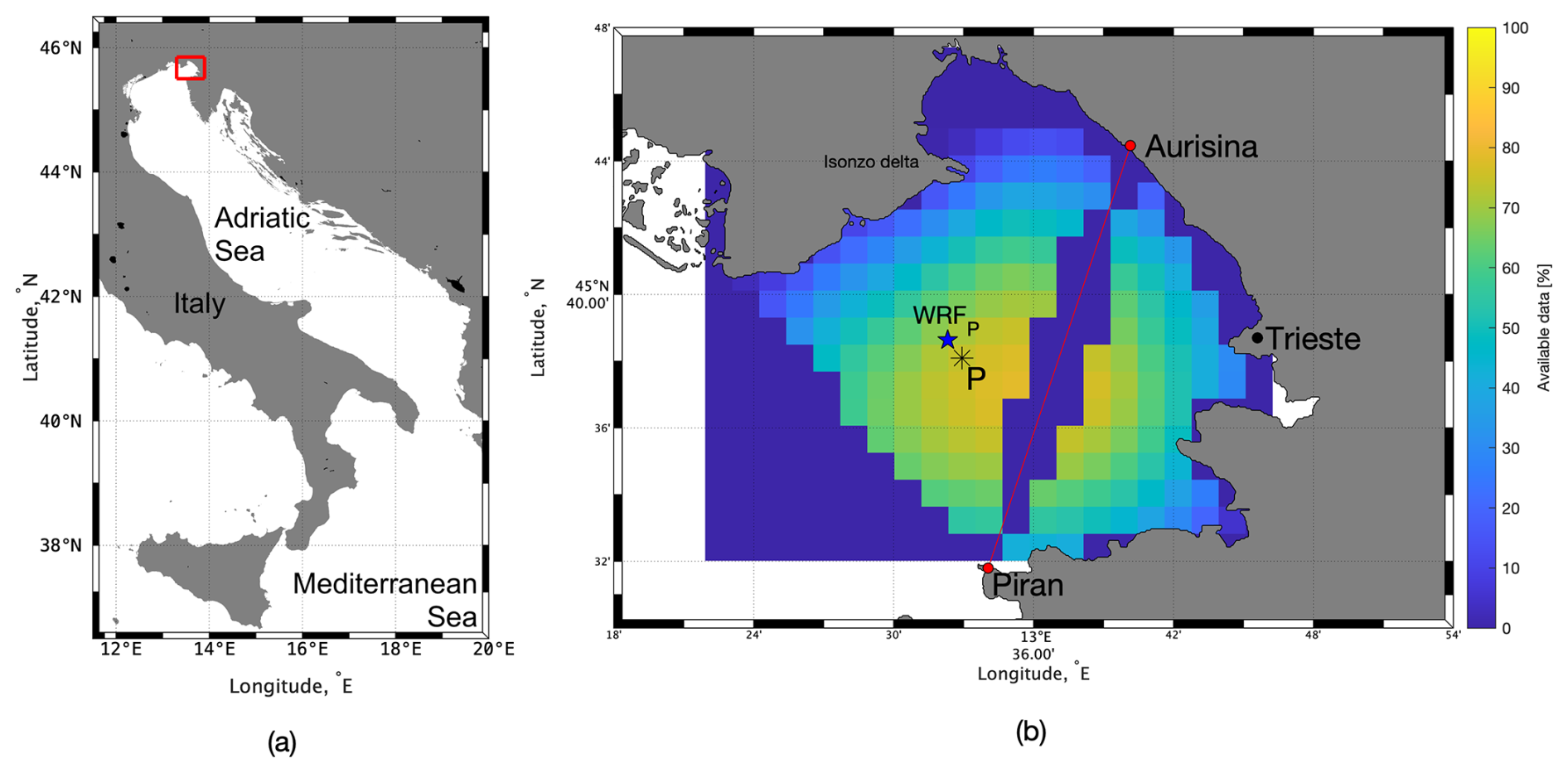
Figure 1 (a) Gulf of Trieste location (red rectangle) in the Adriatic Sea; (b) enlarged view of Gulf of Trieste with the percentage of available HFR data (in multiple colours) for the selected period. The HFR baseline is shown by the red line between Aurisina and Piran. The HFR “P” grid point is shown with a black asterisk, and the closest WRF grid point is marked with a blue star and called “WRF_P” (Flora et al., 2023).

Sea surface currents are measured by two beamforming Wellen Radar stations operating in the Gulf of Trieste (Lorente et al., 2022) (Fig. 1b, red dots). The HFR system combines the radial sea surface currents of the two stations to obtain the longitudinal u and the latitudinal v components, with a spatial resolution of 1.5 km and a time resolution of 30 min. The data are open access; further details can be found in OGS et al. (2023). The quality control standards from the EU high-frequency node (Corgnati et al., 2018) were applied to the data set. In addition, any remaining spikes were removed. The measured u and v time series used in this article are from the P grid point (Fig. 1b).

The atmosphere data consist of the forecasted wind velocity field at 10 m above the surface in the Gulf of Trieste from the Weather Research and Forecasting (WRF) model (https://www.mmm.ucar.edu/models/wrf, last access: 30 October 2024), version 4.2.1. The forecasting is performed daily by the Agenzia Regionale per la Protezione dell'Ambiente del Friuli Venezia Giulia (ARPA FVG) using initial and boundary conditions from the National Oceanic and Atmospheric Administration Global Forecasting System (https://www.ncei.noaa.gov/products/weather-climate-models/global-forecast, last access: 30 October 2024) and provides the wind time series for the same day and the following one. The field has a spatial resolution of 2 km and a temporal resolution of 1 h. Additional technical details can be found in Goglio (2018). The wind components time series used in this article are from the WRF_P grid point (Fig. 1b) and account for the 1 d forecasting.

3 Methods

This section provides the model definition, the FRR background – with details on how it is dealt with within this study – and a methodology to evaluate the predictability of the developed model.

3.1 The model hierarchy

The aim of the present work is to numerically simulate observed sea surface currents with slow dynamics that is governed by the slow components of the forcings and with fast variations that parameterize the remaining, unresolved processes. This is achieved when the time-averaged dynamics and the statistics of the time increments of the model agree with the observation. In the following, the time series prefix “δ” gives the increment time series, $\mathit{\delta }u\left(t\right)=u(t+\mathit{\delta })-u\left(t\right)$, and we call the observed fat-tailed PDF of the sea surface current increments, from Flora et al. (2023), the “Exp-Lin” PDF, as it is composed of an exponential and a linear term.

When modelling a natural process, such as currents, through an SDE, part of the dynamics is resolved, and part of it is parameterized by noise. What is deterministic and what is noise depends on the degree of coarse-graining. In our previous work (Flora et al., 2023), the dynamics was parameterized, and the model has no predictability. The other extreme is a purely deterministic model that includes all the processes involved. Such model is unattainable. We implemented a hierarchy of three idealized local models (two velocity components at one point in space, evolving in time) for the sea surface current in the Gulf of Trieste. The first is the purely deterministic (DET) model, taking into account the tidal signal and the wind-forced Ekman dynamics, while the unresolved processes are neglected. The second is the Gaussian (GAU) model, which adds Gaussian additive stochastic noise for which the corresponding SDE can be solved analytically. The third is the superstatistical (SUP) model, which considers a deterministic signal with the most realistic stochastic noise. The stochastic part of this model is partially resolvable analytically. Furthermore, these models are forced by nine different forcing protocols (FPs) (see Sect. 4). The deterministic and stochastic models come in pairs; the more processes and timescales are resolved deterministically, the less have to be parameterized stochastically.

More precisely, the total sea surface current vector u_o is given in terms of the tidal current u_M, the wind-forced Ekman sea surface current u_E and the stochastic current u_S, as detailed in Table 1 for the different models. The tidal signal is an analytic and linear combination of n tidal components $u_{\mathrm{M}}\left(t\right)={\sum }_{i=\mathrm{1}}^n{a}_{u,i}\cos ({\mathit{\omega }}_{i}t-{\mathit{\varphi }}_{u,i})$ (analogously for v_M), where a, ω and ϕ are the amplitude, the frequency and the phase of each tidal component, respectively.

The Ekman current, subject to the wind forcing, the Coriolis force and the friction with the underlying water masses, is modelled by

$$\begin{array}{}\text{(1)}& {\displaystyle \frac{\mathrm{d}}{\mathrm{d}t}}\left(\begin{array}{c}{u}_{\mathrm{E}}\\ v_{\mathrm{E}}\end{array}\right)=\left(\begin{array}{cc}-\frac{C_B}{\stackrel{\mathrm{̃}}{h}}\stackrel{\mathrm{̃}}{u}& f\\ -f& -\frac{C_B}{\stackrel{\mathrm{̃}}{h}}\stackrel{\mathrm{̃}}{u}\end{array}\right)\left(\begin{array}{c}{u}_{\mathrm{E}}\\ v_{\mathrm{E}}\end{array}\right)+{\displaystyle \frac{\mathrm{1}}{\stackrel{\mathrm{̃}}{h}}}\left(\begin{array}{c}{F}_u\\ F_v\end{array}\right).\end{array}$$

In Eq. (1), C_B=ρ_oc_b, where c_b is the underlying ocean layer drag coefficient; $\stackrel{\mathrm{̃}}{h}={\mathit{\rho }}_{\mathrm{o}}h$, where ρ_o is the ocean density and h is the considered ocean surface layer depth; and $\stackrel{\mathrm{̃}}{u}$ is the total speed of the surface layer as defined in Table 1. The last does not include the tidal current, as it is assumed that the tidal signal is constant along the water column and does not create shear, while the Ekman and stochastic signals are present in the surface layer only. Finally, f is the Coriolis parameter, and $\mathit{F}={\mathit{\rho }}_{\mathrm{a}}{c}_a|{\mathit{u}}_{\mathrm{a}}-{\mathit{u}}_o|({\mathit{u}}_{\mathrm{a}}-{\mathit{u}}_o)$ is the wind forcing (ρ_a is the atmosphere density, c_a the atmosphere drag coefficient and u_a the wind velocity at 10 m above the sea surface). Equation (1) is an ordinary differential equation of the DET model, while it includes the stochastic quantity $\stackrel{\mathrm{̃}}{u}$ in the GAU and SUP models. If the wind forcing were to cease, the modelled mean flow would fall to the tidal signal.

The Ekman modelization in Eq. (1) is valid only on frequency scales comparable to the Coriolis parameter. The stochastic velocity, representing the fast unresolved turbulent dynamics and present in the GAU and SUP models, is defined by the following set of equations (for the purpose of this study, i.e. to reproduce the observed superstatistical statistics, it is sufficient to have uncorrelated stochastic velocity components):

$$\begin{array}{}\text{(2)}& \mathrm{d}\left(\begin{array}{c}x\\ y\end{array}\right)=-{\mathit{\gamma }}_x\left(\begin{array}{c}x\\ y\end{array}\right)\mathrm{d}t+\left(\begin{array}{cc}\sqrt{Q_u}& \mathrm{0}\\ \mathrm{0}& \sqrt{Q_v}\end{array}\right)\left(\begin{array}{c}\mathrm{d}{W}_x\\ \mathrm{d}{W}_y\end{array}\right),\end{array}$$

$$\begin{array}{}\text{(3)}& {\displaystyle \frac{\mathrm{d}}{\mathrm{d}t}}\left(\begin{array}{c}{u}_{\mathrm{S}}\\ v_{\mathrm{S}}\end{array}\right)=-{\mathit{\gamma }}_u\left(\begin{array}{c}{u}_{\mathrm{S}}\\ v_{\mathrm{S}}\end{array}\right)+\mathit{\eta }\left(\begin{array}{c}x\\ y\end{array}\right).\end{array}$$

In Eqs. (2) and (3), the variables dW_x and dW_y are derived from independent Wiener stochastic processes. For every independent realization of the Wiener processes W_x and W_y, we obtain a solution of the dynamics, named a random walker. The collection of all the random walkers forms the stochastic ensemble and allows construction of a PDF. The coefficient ${\mathit{\gamma }}_x=\mathrm{1}/\mathit{\tau }$ is the inverse of the characteristic short timescale τ (short compared to the long timescale discussed below in connection with the SUP model), whose numerical value is determined from the observations (Flora et al., 2023), γ_u is a coefficient that is a posteriori adjusted to obtain the observed HFR initial decay of the autocorrelation function of the SUP model sea surface currents (Fig. 7) and η is a proper constant, as discussed below. The difference between the GAU and SUP models lies in the terms Q. In the GAU model, which is a simplification of the SUP model, Q_u and Q_v are constants: they are the mean values of the SUP model Q variables, as given in Table 1. The GAU model is a system of linear SDEs, and all variables are Gaussian and are determined by their means and variances. All the dependencies for means and variances on the original parameters are given in Appendix A. Furthermore, in Eq. (A33), the analytical condition on η for which the Gaussian variable δu_S has the same mean and variance as x (analogously δv_S with y), given a fixed γ_u, is shown. This also helps to adjust the parameters of the SUP model.

In the SUP model, the Q terms originate themselves from 2ν stochastic processes α_i: $Q={\sum }_{i=\mathrm{0}}^{\mathrm{2}\mathit{\nu }}{\mathit{\alpha }}_i^{\mathrm{2}}$. The variable ν gives the degrees of freedom (DOFs), according to the interpretation of Flora et al. (2023): the system has 1 DOF if its positive variable characterizing the variability of the system maximizes the entropy, i.e. it is exponentially distributed. This corresponds to half the value of the interpretation by Beck and Cohen (2003). Each stochastic process α_i is governed by

$$\begin{array}{}\text{(4)}& \begin{array}{rl}\mathrm{d}{\mathit{\alpha }}_i& =-\mathit{\mu }{\mathit{\alpha }}_i\mathrm{d}t+\mathit{\beta }\mathrm{d}{W}_i,i=\mathrm{1},\mathrm{\cdots },\mathrm{2}\mathit{\nu }\\ & \text{and}\mathit{\beta }=\left\{\begin{array}{l}{\mathit{\beta }}_u\text{for the}u\text{component}\\ {\mathit{\beta }}_v\text{for the}v\text{component},\end{array}\right.\end{array}\end{array}$$

where the variables dW_i are derived from independent Wiener stochastic processes, β_u and β_v are constants whose values are determined empirically, and $\mathit{\mu }=\mathrm{1}/T$ is the inverse of the characteristic long timescale T (i.e. τ≪T), corresponding to the variation timescale of the variance in the superstatistical approach. Its numerical value is determined from the observations (Flora et al., 2023). The variables α_i are solutions of the Langevin equation: they are Ornstein–Uhlenbeck processes (we refer the reader to Kloeden and Platen (1999) for a pedagogical discussion of stochastic processes), characterized by Gaussian statistics:

$$\begin{array}{}\text{(5)}& p_{\mathit{\alpha }}\left({\mathit{\alpha }}_i\right)=\sqrt{{\displaystyle \frac{\mathit{\mu }}{\mathit{\pi }{\mathit{\beta }}^{\mathrm{2}}}}}{e}^{-\mathit{\mu }{\mathit{\alpha }}_i^{\mathrm{2}}/{\mathit{\beta }}^{\mathrm{2}}}.\end{array}$$

In the SUP model, the variables Q depend on the variables ν and α_i, as shown in Table 1. The Q variables are distributed according to a gamma distribution with a shape parameter equal to ν, given in Eq. (B5) and Table B1. In Eq. (B6), we give the computation for its first moment E[Q], used in the GAU model. In Appendix B, the PDFs of the variable x (and y) are derived for ν=2 and $\mathit{\nu }=\mathrm{1}/\mathrm{2}$. A decrease in the stochastic degrees of freedom ν leads to a reduction of the variability (non-maximal entropy) in the unresolved processes, represented by the stochastic variables. In the case of 2 DOF, the variables x and y are Exp-Lin distributed with a PDF given by

$$\begin{array}{}\text{(6)}& \left\{\begin{array}{l}{p}_{\mathit{\nu }=\mathrm{2}}\left(x\right)=\frac{\sqrt{\mathit{\mu }{\mathit{\gamma }}_x}}{\mathrm{2}{\mathit{\beta }}_u}{e}^{-\mathrm{2}\sqrt{\mathit{\mu }{\mathit{\gamma }}_x}\left|x\right|/{\mathit{\beta }}_u}\left(\frac{\mathrm{2}\sqrt{\mathit{\mu }{\mathit{\gamma }}_x}}{{\mathit{\beta }}_u}\left|x\right|+\mathrm{1}\right)\\ p_{\mathit{\nu }=\mathrm{2}}\left(y\right)=\frac{\sqrt{\mathit{\mu }{\mathit{\gamma }}_x}}{\mathrm{2}{\mathit{\beta }}_v}{e}^{-\mathrm{2}\sqrt{\mathit{\mu }{\mathit{\gamma }}_x}\left|y\right|/{\mathit{\beta }}_v}\left(\frac{\mathrm{2}\sqrt{\mathit{\mu }{\mathit{\gamma }}_x}}{{\mathit{\beta }}_v}\left|y\right|+\mathrm{1}\right).\end{array}\right.\end{array}$$

In the case of $\mathrm{1}/\mathrm{2}$ DOF, the variables x and y are distributed according to a modified Bessel function of the second kind of zero-order $K_{\mathrm{0}}\left(\right|z\left|\right)$:

$$\begin{array}{}\text{(7)}& \left\{\begin{array}{l}{p}_{\mathit{\nu }=\frac{\mathrm{1}}{\mathrm{2}}}\left(x\right)=\frac{\mathrm{2}\sqrt{\mathit{\mu }{\mathit{\gamma }}_x}}{\mathit{\pi }{\mathit{\beta }}_u}{K}_{\mathrm{0}}\left(\frac{\mathrm{2}\sqrt{\mathit{\mu }{\mathit{\gamma }}_x}}{{\mathit{\beta }}_u}\left|x\right|\right)\\ p_{\mathit{\nu }=\frac{\mathrm{1}}{\mathrm{2}}}\left(y\right)=\frac{\mathrm{2}\sqrt{\mathit{\mu }{\mathit{\gamma }}_x}}{\mathit{\pi }{\mathit{\beta }}_v}{K}_{\mathrm{0}}\left(\frac{\mathrm{2}\sqrt{\mathit{\mu }{\mathit{\gamma }}_x}}{{\mathit{\beta }}_v}\left|y\right|\right).\end{array}\right.\end{array}$$

The SDEs for the variables u_S and v_S in Eq. (3) contain a linear drag term and are forced by a coloured non-Gaussian noise. We do not know an analytical distribution of u_S and v_S. Nevertheless, thanks to the definition of the constant η in Eq. (A33) discussed in connection with the GAU model, the distributions of δu_S and δv_S are numerically similar to the PDFs of x and y (shown in Sect. 4.1).

As it can be seen in Eqs. (6) and (7), the final stochastic PDFs depend on the β parameter, which is linked to the variable's second-order moment, by $E\left[x^{\mathrm{2}}\right]=\frac{{\mathit{\beta }}^{\mathrm{2}}}{\mathit{\mu }{\mathit{\gamma }}_x}$ for ν=2. For this case, it will be shown in Sect. 4.1 that the PDF of the total velocity increment is given mainly by the stochastic velocity increment PDF only. For this reason, in the numerical simulations with 2 DOF in the stochastic part of the model, the value of β is therefore fixed by the observed variance s² of the HFR velocity increment found in Flora et al. (2023): $\mathit{\beta }=s\sqrt{\mathit{\mu }{\mathit{\gamma }}_x}$. In the case of $\mathrm{1}/\mathrm{2}$ DOF in the stochastic signal, the tidal and Ekman signals contribute more to the variance of the total velocity increment, but their contribution is unknown analytically. For this reason, in this case, the β coefficient is increased empirically in order to fit the observed variance in the total velocity increment PDF.

Table 1 Variable definitions distinguishing the different models and the x, y, δu_S and δv_S PDFs' characteristics. The variable ν indicates the degrees of freedom of the stochastic signal.

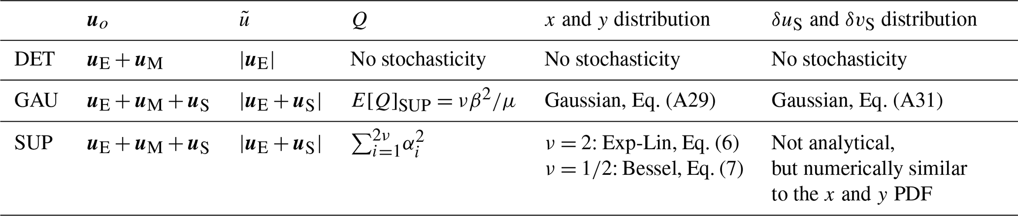
In Table 1, the definitions of the variables distinguishing the DET, GAU and SUP models are given with a summary of the main properties of the models' variables. For all the models, we can (or cannot) consider the eddy depletion term in the wind stress term, i.e. the relative velocity of the wind with respect to the sea surface current, causing a reduction of kinetic energy injection into the ocean (Zhai et al., 2012), in contrast to the absolute wind velocity. We report the results just with the eddy depletion term, as it is the theoretically most correct formulation and does not significantly burden the computational calculation.

In summary, we developed three types of models: the DET model is purely deterministic with tidal and Ekman currents, the GAU model adds a Gaussian stochastic signal, and the SUP model considers a stochastic sea surface current with fat-tailed increments instead of the Gaussian noise (Table 1).

3.2 The FRR background and methods

The FRR relates the response of a system perturbed by an external perturbation to internal fluctuations of the unperturbed system. Exploring the FRR is particularly challenging and interesting when considering natural systems where perturbation experiments cannot be performed and statistical ensembles are not available. Our SUP model is an example of a subcomponent of the climate system, and it is instructive to explore the FRR for such model. We refer to Lacorata and Vulpiani (2007) for the theoretical background concerning FRRs. We show here some fundamentals of the theoretical concepts and the methodology we applied to the most involved of the SUP models (FP9, Table 2, Sect. 4).

In the present case, given the SUP model evolutionary system with the SUP variables $u_o=u_{\mathrm{E}}+u_{\mathrm{M}}+u_{\mathrm{S}}$ and $v_o=v_{\mathrm{E}}+v_{\mathrm{M}}+v_{\mathrm{S}}$, a small fixed perturbation Δu_S or Δv_S is imposed at t=t₀ to each walker. Then, the system is left free to evolve and, for each time, the separation $\mathrm{\Delta }{u}_o\left(t\right|t_{\mathrm{0}})=u_{o,\mathrm{P}}(t)-u_o(t)$ and $\mathrm{\Delta }{v}_o\left(t\right|t_{\mathrm{0}})=v_{o,\mathrm{P}}(t)-v_o(t)$ between the perturbed (u_o,P and v_o,P) and the unperturbed (u_o and v_o) systems is computed. We emphasize that the methodology requires one velocity component to be perturbed and not both in the same perturbed simulation. It is possible to obtain the mean value of the perturbed variables through a mean response function R_uu(t) or R_vv(t):

$$\begin{array}{}\text{(8)}& \begin{array}{rl}\langle \mathrm{\Delta }{u}_o\left(t\right)\rangle & =R_{uu}\left(t\right)\mathrm{\Delta }{u}_{\mathrm{S}}\text{when }{u}_{\mathrm{S}}\text{ is perturbed}\\ \langle \mathrm{\Delta }{v}_o\left(t\right)\rangle & =R_{vv}\left(t\right)\mathrm{\Delta }{v}_{\mathrm{S}}\text{when }{v}_{\mathrm{S}}\text{ is perturbed},\end{array}\end{array}$$

where the angle brackets 〈⋯〉 indicate the ensemble mean. The FRR is concerned with expressing the mean response function in terms of correlation functions of the unperturbed system.

In practice, the mean response functions are computed as follows. After the first perturbation at t₀, the selected variable in the perturbed system is perturbed again with the same variation at $t_k=t_{\mathrm{0}}+k\mathrm{\Delta }t$, and the separation between the perturbed and unperturbed systems is computed. The perturbation time is fixed to Δt=12 h, allowing us to repeat the procedure $M=\mathrm{1311}\gg \mathrm{1}$ times, and $\mathrm{\Delta }{u}_{\mathrm{S}}=\mathrm{\Delta }{v}_{\mathrm{S}}=\mathrm{8}$ cm s⁻¹. The diagonal mean response functions are computed as follows:

$$\begin{array}{}\text{(9)}& \begin{array}{rl}{R}_{uu}\left(t\right)& ={\displaystyle \frac{\mathrm{1}}{M}}\sum _{k=\mathrm{0}}^{M-\mathrm{1}}{\displaystyle \frac{\langle \mathrm{\Delta }{u}_o(t_k+t|t_k)\rangle }{\mathrm{\Delta }{u}_{\mathrm{S}}}}\text{when }{u}_{\mathrm{S}}\text{ is perturbed}\\ R_{vv}\left(t\right)& ={\displaystyle \frac{\mathrm{1}}{M}}\sum _{k=\mathrm{0}}^{M-\mathrm{1}}{\displaystyle \frac{\langle \mathrm{\Delta }{v}_o(t_k+t|t_k)\rangle }{\mathrm{\Delta }{v}_{\mathrm{S}}}}\text{when }{v}_{\mathrm{S}}\text{ is perturbed}.\end{array}\end{array}$$

According to Lacorata and Vulpiani (2007), the FRR holds if the mean response functions have a connection with some suitable correlation functions computed in the unperturbed system. In particular, in the case of multivariate Gaussian variables, the mean response functions are a linear combination of the variable correlations. In Sect. 4.2, the results with unperturbed initial condition ${\mathit{u}}_o(t=\mathrm{0})=\mathrm{0}$ and when the stochastic signal is initially perturbed, as described before, is shown. Some brief comments for the case where the Ekman system is initially perturbed are also provided.

3.3 Predictability evaluation methods

In order to test the predictability capabilities of the SUP model, perturbation methods are adopted assuming that the HFR observations are not affected by observational uncertainty and represent the reality, i.e. modelled data are replaced by observations. In the following, this method is called “observation-based perturbation”. In detail, at every time Δt, the perturbed system (u_o,P) is updated to the observed HFR velocities (both the u_o and v_o components in the same simulation); in particular, it is the stochastic signal to be perturbed. The method may appear equivalent to the FRR method, but the equivalence is not valid because (i) the initial perturbation is not a constant but changes for each Δt time window and for each walker and (ii) we are perturbing both the u_o and v_o components (in the stochastic signal) in the same perturbed simulation. We define the following functions:

$$\begin{array}{}\text{(10)}& {\displaystyle }\mathit{\xi }\left(t\right)=\sqrt{{\displaystyle \frac{\frac{\mathrm{1}}{M}{\sum }_{k=\mathrm{0}}^{M-\mathrm{1}}\langle {\left({\mathit{u}}_{o,\mathrm{P}}(t_k+t)-{\mathit{u}}_o(t_k+t)\right)}^{\mathrm{2}}\rangle }{\frac{\mathrm{1}}{M}{\sum }_{k=\mathrm{0}}^{M-\mathrm{1}}\langle {\left({\mathit{u}}_{o,\mathrm{P}}(t_{k-\mathrm{1}}+\mathrm{\Delta }t)-{\mathit{u}}_{\text{HFR}}\left(t_k\right)\right)}^{\mathrm{2}}\rangle }}},\text{(11)}& {\displaystyle }\mathit{ϵ}\left(t\right)=\sqrt{{\displaystyle \frac{\frac{\mathrm{1}}{M}{\sum }_{k=\mathrm{0}}^{M-\mathrm{1}}\langle {\left({\mathit{u}}_{o,\mathrm{P}}(t_k+t)-{\mathit{u}}_{\text{HFR}}(t_k+t)\right)}^{\mathrm{2}}\rangle }{\frac{\mathrm{1}}{M}{\sum }_{k=\mathrm{0}}^{M-\mathrm{1}}\langle {\left({\mathit{u}}_{o,\mathrm{P}}(t_{k-\mathrm{1}}+\mathrm{\Delta }t)-{\mathit{u}}_{\text{HFR}}\left(t_k\right)\right)}^{\mathrm{2}}\rangle }}},\end{array}$$

where the time $t_{k-\mathrm{1}}+\mathrm{\Delta }t$ means t_k right before the perturbation. The function ξ(t) quantifies the difference between the perturbed and the unperturbed system, while the function ϵ(t) computes the difference between the perturbed system and the observations. Both are normalized through the mean initial perturbation over all the time windows. In Sect. 4.3, the results are presented. Some brief comments for the case where the Ekman system is initially perturbed are also provided.

4 Results and discussion

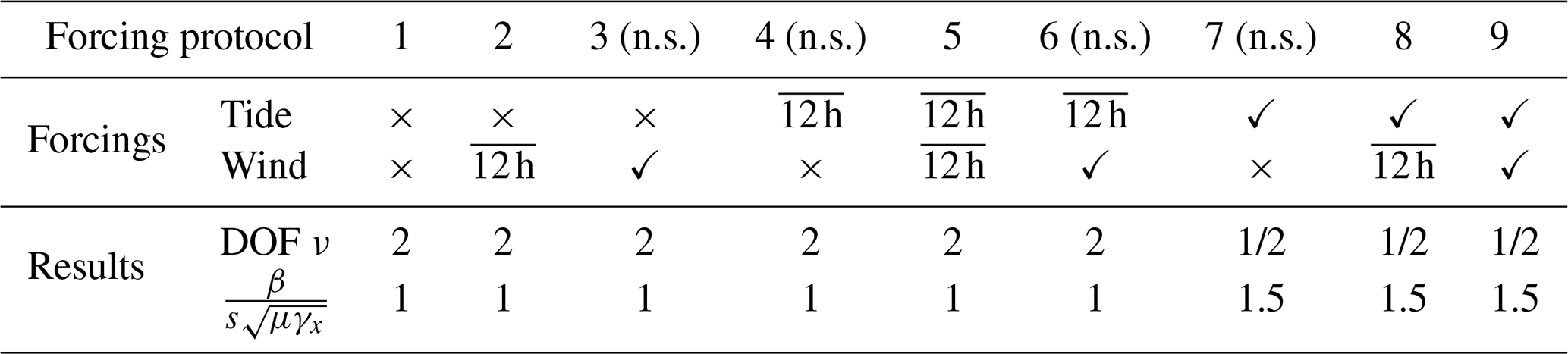
We test the different models by imposing different forcing protocols (FPs) in the tidal and wind time series (Table 2). In the most complete FP, the complete tidal and wind forcing is included (FP9); in the other FPs, the forcing signal is either averaged by a moving average over 12 h or completely set to zero.

Table 2 Settings and results of the experiments on the models: × means that the forcing is set to 0, $\stackrel{\mathrm{‾}}{\mathrm{12}\mathrm{h}}$ means that the forcing is filtered with a 12 h moving average and ✓ means that we use the original forcing. The variable s is the observed standard deviation of the HFR velocity increment found in Flora et al. (2023). The abbreviation “n.s.” stands for “not shown”.

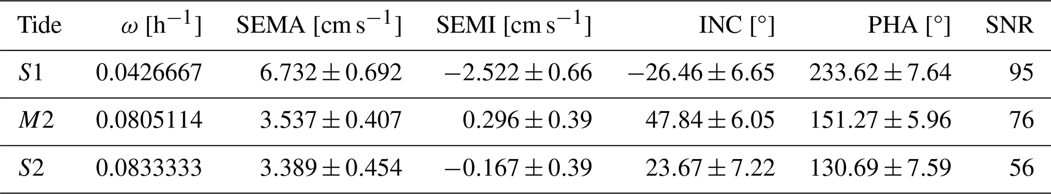
The numerical values of the coefficients common to all the models and to all the runs are described here. Tidal harmonic analysis calculations on the HFR sea surface currents were done using the MATLAB programme t_tide (Pawlowicz et al., 2002). The resultant tidal ellipse parameters are shown in Table 3. The S1, M2 and S2 tidal components show a sufficiently high signal-to-noise ratio (SNR) and are therefore included to be considered in our modelization. The conversion from the ellipse parameters to the sinusoidal tidal coefficients is applied according to Foreman (1978). The non-filtered tidal signal consists of the S1, M2 and S2 components, while the 12 h moving-averaged signal is characterized by the diurnal oscillation only.

Table 3 Tidal ellipse parameters with 95 % confidence interval estimates, extracted from the HFR data.

The wind velocity u_a time series is linearly interpolated from its 1 h original resolution or from a 12 h moving average to the integration time step of the numerical model (2.5 min). The determination of $\stackrel{\mathrm{̃}}{h}$ and C_B as best linear fit functions of the wind speed is given in Appendix C. The algorithm to determine the wind regimes Bora, Sirocco, Mistral and low wind is explained in Flora et al. (2023): if the daily wind speed is higher than the threshold value of 3 m s⁻¹, then it is defined as Bora, Sirocco or Mistral depending on its direction; if it is lower, it is classified as low wind. Mistral occurs just for a few days in almost 2 years; it is therefore considered statistically not significant. In the numerical integration, the parameters shown in Table 4 are used, and a Runge–Kutta method of the second order is adopted for the Ekman system.

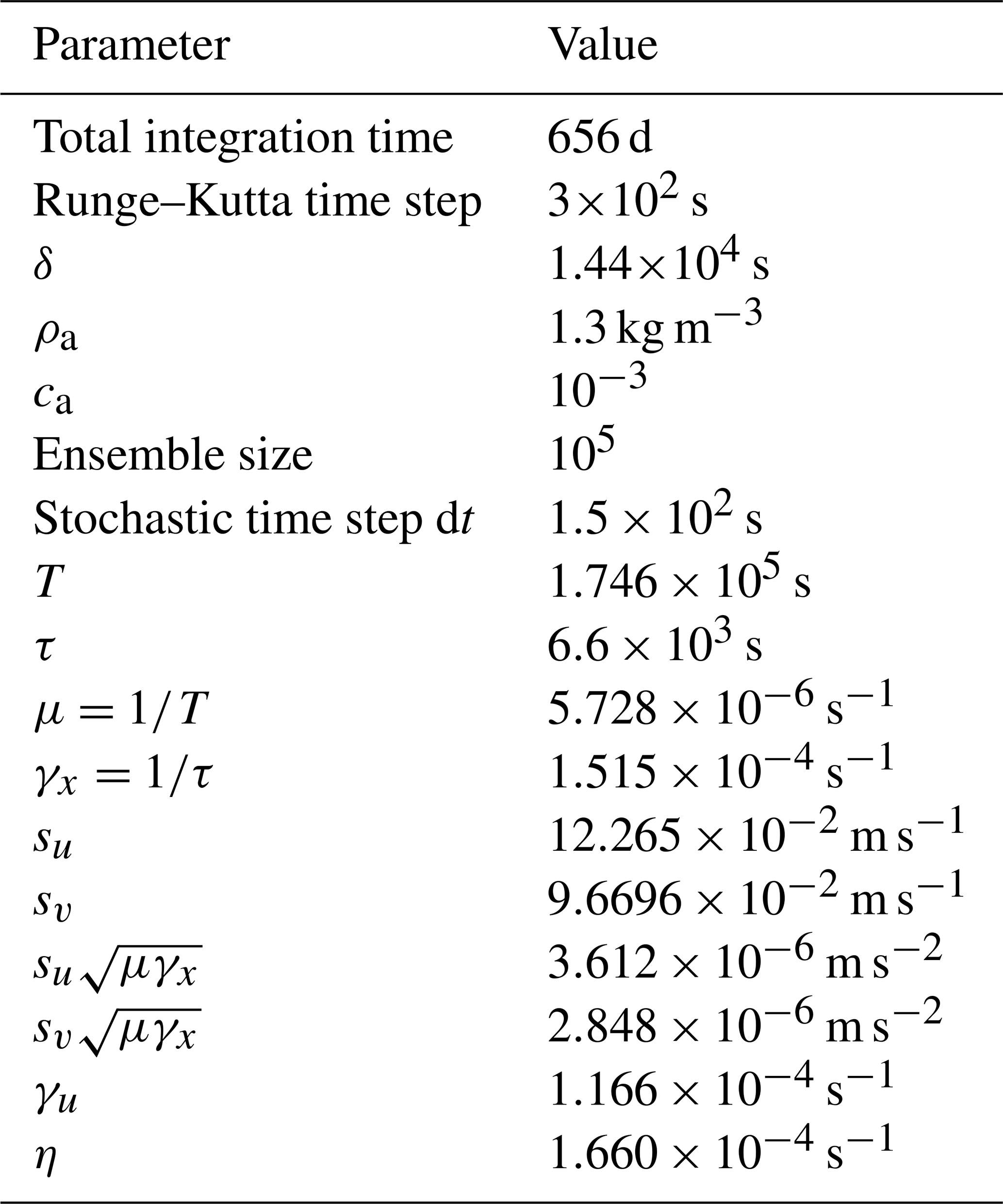
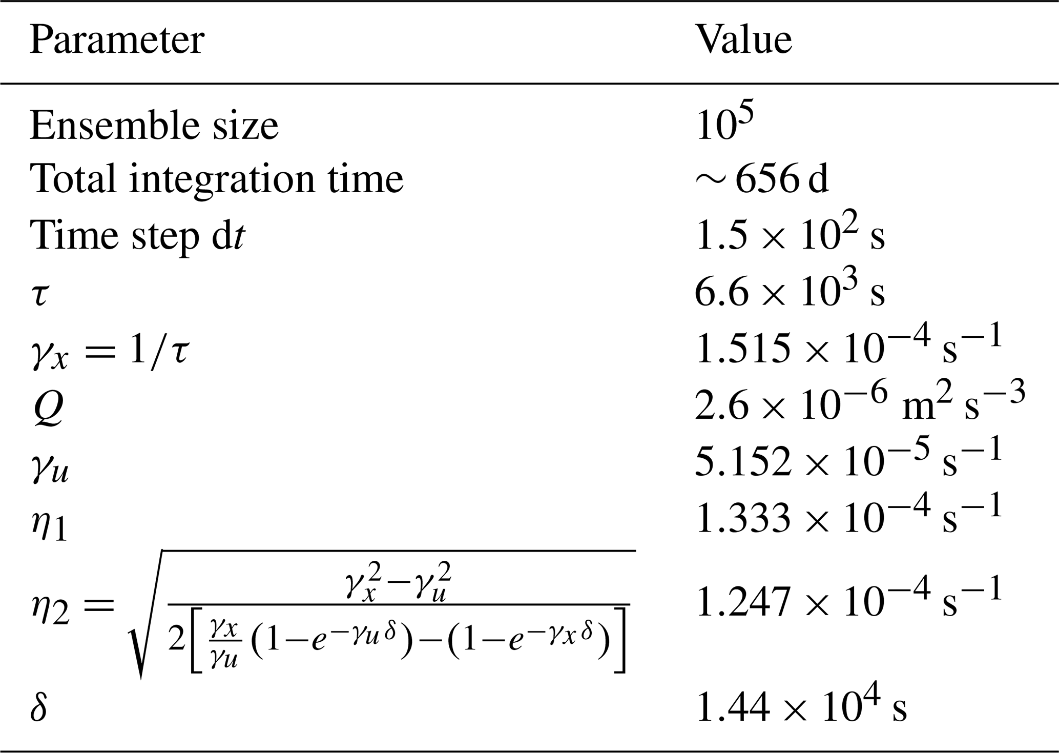
Table 4 Parameters involved in the numerical modelization: total integration time, Runge–Kutta time step, increment time δ (from the velocity increment definition), atmosphere density ρ_a, atmosphere drag coefficient c_a, ensemble size, stochastic time step dt, long timescale T, short timescale τ, α_i's linear drag coefficient μ, x's and y's linear drag coefficient γ_x, observed HFR velocity increments' standard deviations s_u and s_v, u_S's and v_S's linear drag coefficient γ_u, and forcing coefficient η. The numerical values of δ, τ, T, s_u and s_v are taken from Flora et al. (2023).

4.1 Comparison of the DET, GAU and SUP models on different forcing timescales

All the models start from the initial condition ${\mathit{u}}_o(t=\mathrm{0})={\mathit{u}}_{\text{HFR}}(t=\mathrm{0})$, where u_HFR is the observed HFR sea surface velocity, with ${\mathit{u}}_{\mathrm{S}}(t=\mathrm{0})=\mathrm{0}$. The obtained numerical sea surface currents are then compared to the HFR measurements. We start this section by commenting on FP1, which has no tides and no wind forcing (see Table 2), and compare the DET, GAU and SUP models in the FP5 and FP9 cases (see Table 2). We conclude this section with a discussion of the change in the stochastic DOF when the tidal forcing is modified. We show only time series for the u component of the sea surface current variables; the results for the v component are similar.

The stochastic model has to be adapted to the FPs to best represent the dynamics unresolved by the deterministic part of the model. FP1 does not take into account any physical forcings, and the deterministic part vanishes. The DET model is therefore null, while the GAU and SUP models have a nonzero stochastic part. The SUP model best fits the observed data when ν=2 DOF is chosen (see Flora et al., 2023), as we obtain a total velocity increment (δu_o=δu_S because, in FP1, $\mathit{\delta }{u}_{\mathrm{M}}=\mathit{\delta }{u}_{\mathrm{E}}=\mathrm{0}$) distributed according to the Exp-Lin PDF (as summarized in Table 1). The result is shown in the left column of Fig. 2, in which SUP δu_o of FP1 coincides with SUP δu_S of FP5 (as shown in Table 2 and commented on below, they both have ν=2 stochastic DOF). The GAU model in FP1 (Eq. (A31) and the left column of Fig. 2, in which GAU δu_o of FP1 coincides with GAU δu_S of FP5) fails in reproducing the fat-tailed Exp-Lin PDF.

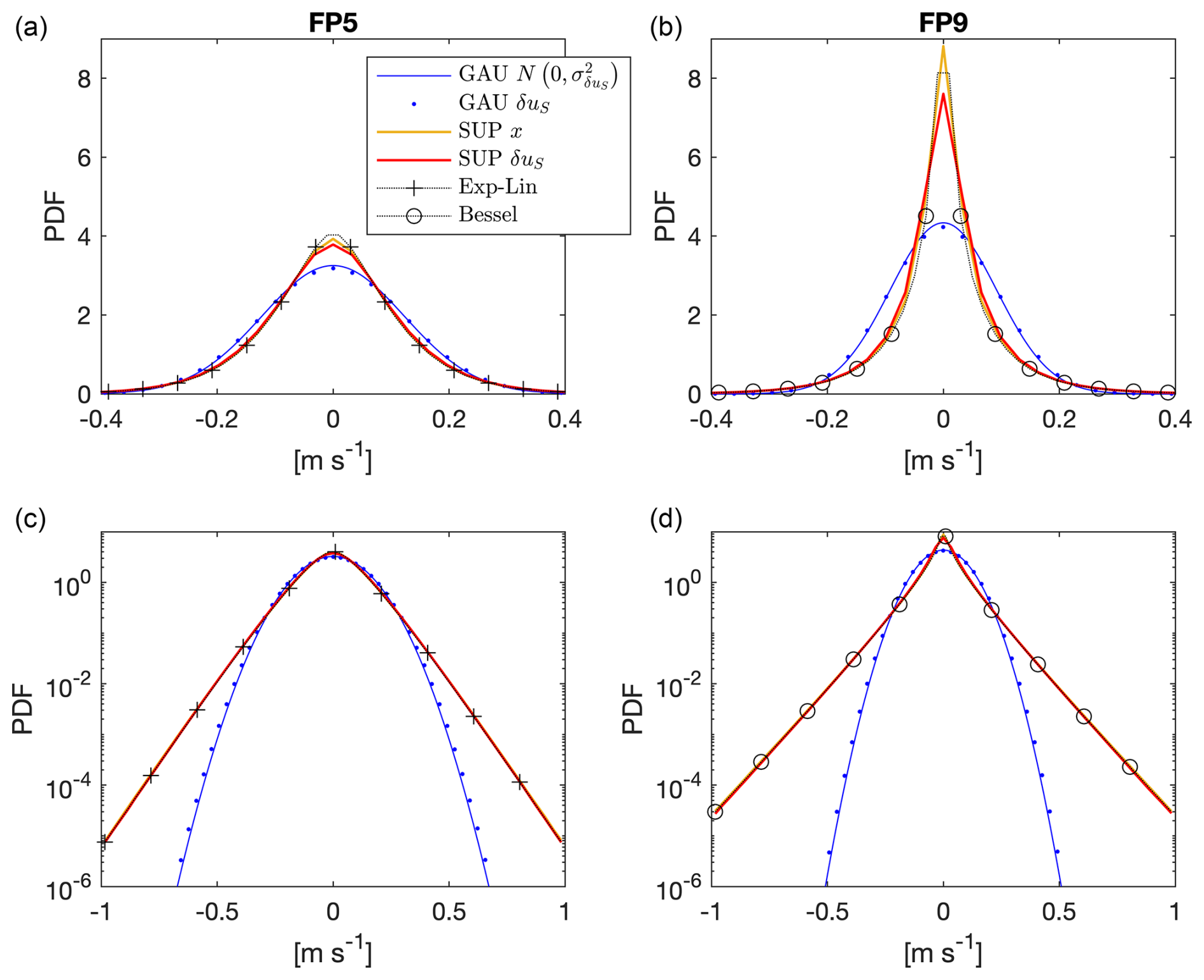
Figure 2 PDFs of the stochastic variables of the GAU and SUP models for FP5 (left column) and FP9 (right column) in lin–lin plots (top row) and lin–log plots (bottom row). In particular, analytical solution of the GAU δu_S variable from Eq. (A31) (blue continuous line) and PDFs of the model variables: numerical GAU δu_S (blue dots), SUP x (yellow continuous line) and SUP δu_S (red continuous line). PDFs of the analytical superstatistical Exp-Lin PDF from Eq. (6) (black dotted line with crosses) and of the analytical superstatistical Bessel function from Eq. (7) (black dotted line with circles) are also shown. Note that in FP5 (FP9), the SUP x, SUP δu_S and Exp-Lin (Bessel) lines almost superpose.

In FP5, a 12 h moving-averaged tidal and wind forcing is applied to the models, while FP9 includes the forcings without averaging (see Table 2). For the different types of forcings, we choose the DOF that best fitted the superstatistical Exp-Lin PDF from Flora et al. (2023). In particular, for FP5, ν=2 gives the best fits, while for FP9, $\mathit{\nu }=\mathrm{1}/\mathrm{2}$ does. In Fig. 2, the PDFs of the stochastic variables of the GAU and SUP models for FP5 and FP9 are compared to the analytical PDFs. The figures validate the choice of the parameters in our model hierarchy for the different forcings, as summarized in Table 1: (i) the GAU δu_S follows the analytical Gaussian from Eq. (A31); (ii) in FP5, the stochastic variable SUP x is Exp-Lin distributed, while in FP9, it is Bessel distributed; (iii) the SUP δu_S are distributed as SUP x in both the simulations, showing the validity of the choice of η (fixed according to the analytical condition from the GAU model in Eq. (A33) – its choice is discussed in Sect. 3.1 in connection with the GAU and SUP models). This also validates the numerical model through the cases where the analytical solution is known.

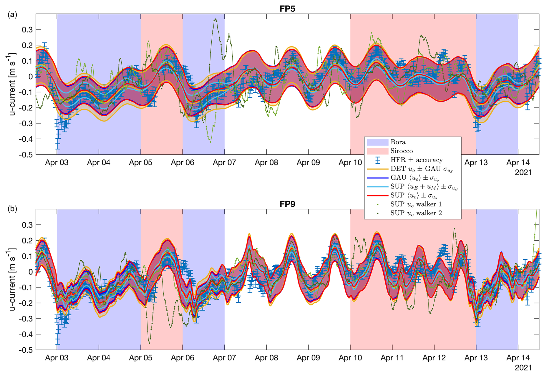
Figure 3 Sea surface currents time series (u component) during 11 d in April 2021 of the HFR observations with their measurement accuracy (blue sticks with error bars) from the models for FP5 (a) and for FP9 (b): DET model u_o with the Gaussian GAU model ensemble standard deviation of the stochastic velocity (yellow lines), GAU model ensemble mean of u_o with their ensemble standard deviation (blue lines), SUP model ensemble mean of u_E+u_M with their ensemble standard deviation (light-blue lines) and SUP model ensemble mean of u_o with their ensemble standard deviation (red lines). The SUP u_o path of two random walkers is reported (light- and dark-green dotted lines). The symbol 〈⋯〉 in the legend stands for the ensemble mean. The blue and red shadings represent the Bora and Sirocco wind regimes, respectively, seen in Flora et al. (2023).

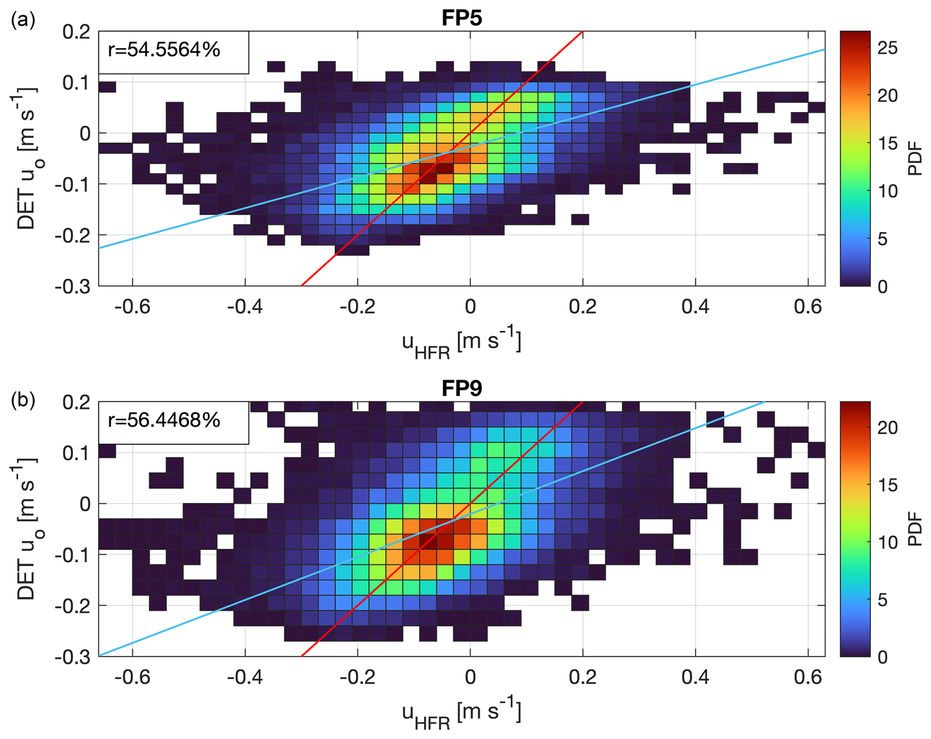
Figure 4 Normalized 2D histograms of the correlation between the HFR observations and the DET model u-component velocities from the simulated period (almost 2 years) from FP5 (a) and from FP9 (b). The r correlation coefficient is reported. The light-blue line is the linear regression of the scattered data, while the red line is the bisector.

In Fig. 3, the time series of the observed and model velocities for some days of April 2021 are reported. The difference in the forcing timescale is clearly visible in the deterministic DET model velocities' variability: smoother in FP5 than in FP9. They both follow the slow variability of the observed HFR currents. In fact, looking at Fig. 4, the linear regression of the scattered data has a lower slope with respect to the bisector, meaning that the DET model is not able to simulate the observed extremes. Nevertheless, their 2D histograms have an elongated peak along the bisector, and their correlation coefficient reaches 55 % in FP5 and 56 % in FP9 for the u component (29 % and 35 % for the v component, respectively). Moreover, it is possible to see that sometimes (e.g. 3 April 2021 from Fig. 3) the observed u_HFR sea surface current shows a negative peak at the beginning of Bora events. This behaviour is missing from the DET model u_o velocity. This fact can be due to the model instantaneous change in the values of $\stackrel{\mathrm{̃}}{h}$ and C_B with the wind speed, while the sea surface system in nature takes some time to adjust to the wind forcing through vertical mixing (the thin surface layer suddenly accelerates, then thickens, and the speed decreases).

Regarding the ensemble averaged sea surface currents of the GAU and SUP models, they follow closely the DET model time series. This shows that the stochastic models increase the variability to observed values but have little influence on the averaged dynamics. We emphasize that if our model were perfect, the observations would be one of the walkers and therefore would at times be outside the SUP total velocity ensemble standard deviation ${\mathit{\sigma }}_{u_o}$ (red) band, as is the case for the two random walkers (green lines) reported in Fig. 3. The SUP ensemble standard deviation of the u_E+u_M velocity (light-blue band) is smaller than the SUP total velocity ensemble standard deviation ${\mathit{\sigma }}_{u_o}$ (red band), as expected, because the tidal velocity is purely deterministic and, in the Ekman velocity, the stochasticity enters only through the drag. What is particularly interesting is that the GAU ${\mathit{\sigma }}_{u_o}$ ensemble standard deviation (blue band) almost completely coincides with the SUP ${\mathit{\sigma }}_{u_o}$ (red band) and not with the GAU ${\mathit{\sigma }}_{u_{\mathrm{S}}}$ (yellow band) ensemble standard deviation. A clear example of that is visible on 3, 4, 6 and 13 April 2021 in Fig. 3 for the u component, where the wind forcing increases and the GAU and SUP ${\mathit{\sigma }}_{u_o}$ standard deviations (blue and red bands, respectively) reduce with respect to the GAU ${\mathit{\sigma }}_{u_{\mathrm{S}}}$ statistics (yellow band). In this case, it originates from the stochasticity present in the Ekman drag term.

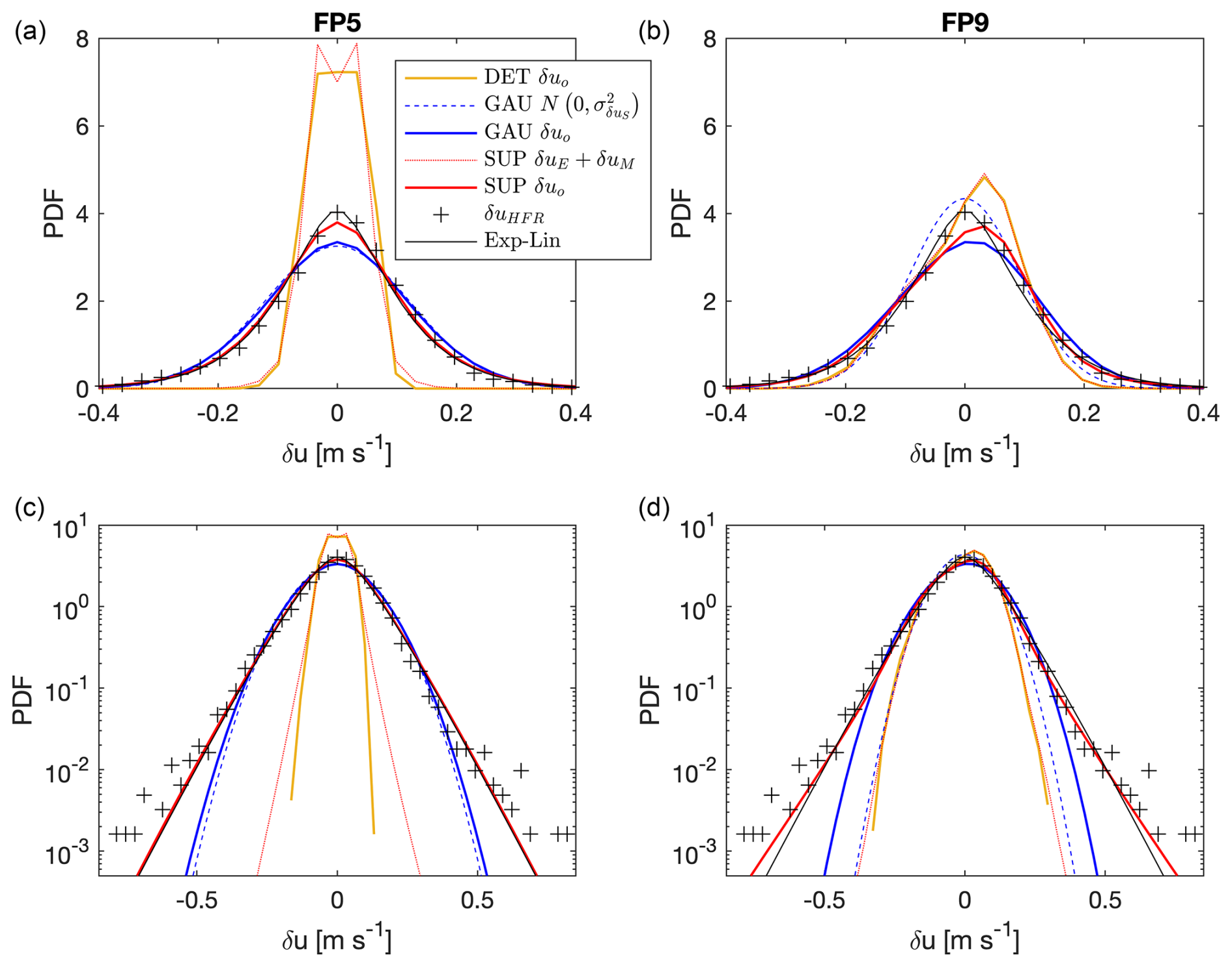
Figure 5 PDFs of the observed, analytical and numerical velocity increments from FP5 (a, c) and FP9 (d, b) in lin–lin plots (a, b) and lin–log plots (c, d). In particular, we show the PDFs of the observed HFR velocity increment (black crosses), of the analytical superstatistical PDF from Eq. (6) (black line), of the analytical Gaussian of the GAU δu_S variable from Eq. (A31) (blue dashed line) and of the model variables: DET δu_o (yellow line), GAU δu_o (blue line), SUP δu_E+δu_M (red dotted line) and SUP δu_o (red solid line).

Looking at the PDFs of the velocity increments in Fig. 5, it can be seen that the DET model PDF in FP5 is more peaked around zero compared to FP9, which is closer to the observations. This is because the latter model has a higher variability due to the inclusion of higher-frequency forcing data. Despite the rather high correlation of the DET currents with the observations, the DET model does not explain most of the variability seen in the HFR data, especially the tails, i.e. the extreme events, which are not well reproduced.

From Fig. 5, one can also observe that in FP5, the GAU δu_o PDF is similar to the analytical PDF $N(\mathrm{0},{\mathit{\sigma }}_{\mathit{\delta }{u}_{\mathrm{S}}})$ from Eq. (A31), while in FP9, it deviates, showing a lower peak and fat tails. The reason is explained in more detail for the SUP model in the next paragraph, but, in summary, it is due to the capacity in FP9 of the tidal and Ekman modelization to resolve a large part of the variability. For both FPs, although the first and second moments of the velocities are comparable to the SUP model (Fig. 3) and the shape of the PDF of the velocity increments has improved compared to the results of the DET model (Fig. 5), the tails of the GAU velocity increment PDFs are (by construction) not fat enough to resemble the superstatistical Exp-Lin PDF, and the occurrence of extreme events is strongly underestimated.

Regarding the SUP model, in FP5, the SUP δu_E+δu_M PDF is very peaked, due to the 12 h forcing timescale that suppresses a large part of the variability. Hence, the SUP δu_E+δu_M PDF contributes little to the SUP δu_o PDF, which is distributed similar to the SUP δu_S Exp-Lin PDF, having fat tails (compare Figs. 2 and 5). In FP9, the SUP δu_E+δu_M PDF is distributed closely to the DET δu_o PDF (larger with respect to the FP5 case), meaning that a large part of the SUP δu_o variability is resolved by the deterministic model. The SUP δu_S PDF is given by the Bessel function of Eq. (7) and shown in Fig. 2. The SUP δu_o PDF, shown in Fig. 5, is a convolution of the SUP δu_E+δu_M PDF (no analytical form available) and the Bessel function. This PDF shows a lower and shifted peak with respect to the observed and superstatistical Exp-Lin PDFs (probably due to the SUP δu_E+δu_M PDF), but its tails slightly deviate from the observed and Exp-Lin ones.

The percentages of the observed HFR velocity increments inside the SUP ${\mathit{\sigma }}_{\mathit{\delta }{u}_o}$ (and ${\mathit{\sigma }}_{\mathit{\delta }{v}_o}$) ensemble standard deviation band are measured from the model results:

$$\begin{array}{}\text{(12)}& {\displaystyle }\text{FP5}\left\{\begin{array}{l}\mathrm{Pr}{\left(\mathit{\delta }{u}_o-{\mathit{\sigma }}_{\mathit{\delta }{u}_o}\le \mathit{\delta }{u}_{\mathrm{HFR}}\le \mathit{\delta }{u}_o+{\mathit{\sigma }}_{\mathit{\delta }{u}_o}\right)}_{\mathrm{SUP}}^{\mathrm{FP}\mathrm{5}}\simeq \mathrm{73}\mathit{\%}\\ \mathrm{Pr}{\left(\mathit{\delta }{v}_o-{\mathit{\sigma }}_{\mathit{\delta }{v}_o}\le \mathit{\delta }{v}_{\mathrm{HFR}}\le \mathit{\delta }{v}_o+{\mathit{\sigma }}_{\mathit{\delta }{v}_o}\right)}_{\mathrm{SUP}}^{\mathrm{FP}\mathrm{5}}\simeq \mathrm{73}\mathit{\%},\end{array}\right.\text{(13)}& {\displaystyle }\text{FP9}\left\{\begin{array}{l}\mathrm{Pr}{\left(\mathit{\delta }{u}_o-{\mathit{\sigma }}_{\mathit{\delta }{u}_o}\le \mathit{\delta }{u}_{\mathrm{HFR}}\le \mathit{\delta }{u}_o+{\mathit{\sigma }}_{\mathit{\delta }{u}_o}\right)}_{\mathrm{SUP}}^{\mathrm{FP}\mathrm{9}}\simeq \mathrm{61}\mathit{\%}\\ \mathrm{Pr}{\left(\mathit{\delta }{v}_o-{\mathit{\sigma }}_{\mathit{\delta }{v}_o}\le \mathit{\delta }{v}_{\mathrm{HFR}}\le \mathit{\delta }{v}_o+{\mathit{\sigma }}_{\mathit{\delta }{v}_o}\right)}_{\mathrm{SUP}}^{\mathrm{FP}\mathrm{9}}\simeq \mathrm{62}\mathit{\%}.\end{array}\right.\end{array}$$

Repeating the calculation in Eq. (12) and Eq. (13) without the eddy depletion term, we obtain a difference of less than 1 % with respect to the shown case, in which the relative velocity between the sea and the atmosphere is considered. For FP5, the percentages compare well to the analytical superstatistical Exp-Lin values:

$$\begin{array}{}\text{(14)}& \begin{array}{rl}\mathrm{Pr}(-\mathit{\sigma }\le x\le \mathit{\sigma })& =\underset{-\mathit{\sigma }}{\overset{+\mathit{\sigma }}{\int }}{\displaystyle \frac{e^{-\mathrm{2}\left|x\right|/\mathit{\sigma }}\left(\frac{\mathrm{2}\left|x\right|}{\mathit{\sigma }}+\mathrm{1}\right)}{\mathrm{2}\mathit{\sigma }}}\mathrm{d}x\\ & =\underset{\mathrm{0}}{\overset{+\mathit{\sigma }}{\int }}{\displaystyle \frac{e^{-\mathrm{2}x/\mathit{\sigma }}\left(\frac{\mathrm{2}x}{\mathit{\sigma }}+\mathrm{1}\right)}{\mathit{\sigma }}}\mathrm{d}x\\ & ={\displaystyle \frac{\mathrm{1}}{\mathrm{2}}}\underset{\mathrm{0}}{\overset{\mathrm{2}}{\int }}{e}^{-z}(z+\mathrm{1})\mathrm{d}z\simeq \mathrm{73}\mathit{\%}.\end{array}\end{array}$$

This fact quantitatively confirms that the SUP model in FP5 needs ν=2 DOF in the stochastic signal, producing a reliable PDF with respect to the observations. In this respect, the observations are therefore indistinguishable from a single walker of the SUP model ensemble. The percentages of the FP9 case, which has $\mathit{\nu }=\mathrm{1}/\mathrm{2}$ DOF in the stochastic signal, show small discrepancies with respect to the analytical ones. Despite the deviations from the analytical superstatistical Exp-Lin PDF, the SUP model in FP9 reproduces the PDF tails of the velocity increments with even greater fidelity to the observations than in the FP5 case (Fig. 5).

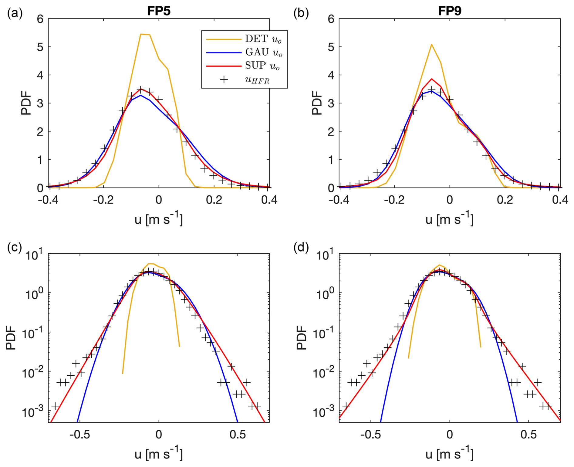
Figure 6 PDFs of the observed u_HFR (black crosses) and numerical model sea surface currents from FP5 (a, c) and FP9 (b, d) in lin–lin plots (a, b) and lin–log plots (c, d): DET u_o (yellow line), GAU u_o (blue line) and SUP u_o (red line).

We now move our attention from the PDFs of the velocity increments to the PDFs of the velocities (Fig. 6). The DET model is not able to represent the observed PDFs, with FP5 clearly missing the most of the variability and FP9 (full forcing) improving the situation but still not reproducing the fat tails. A stochastic part is needed to represent unresolved processes and to increase the variability. The GAU and SUP models can better reproduce the observations. The GAU model shows a good pattern around the peak, while it fails in the reproduction of the extreme events, with errors of around 1 and 3 orders of magnitude for the occurrence of extreme velocities of 0.5 m s⁻¹ in FP5 and FP9, respectively. The SUP model in FP5 confirms, also with this variable, that it can capture the observed statistics. In FP9, the SUP model shows a higher peak but demonstrates the ability to reproduce some details that FP5 cannot, as the PDF decays with two different slopes.

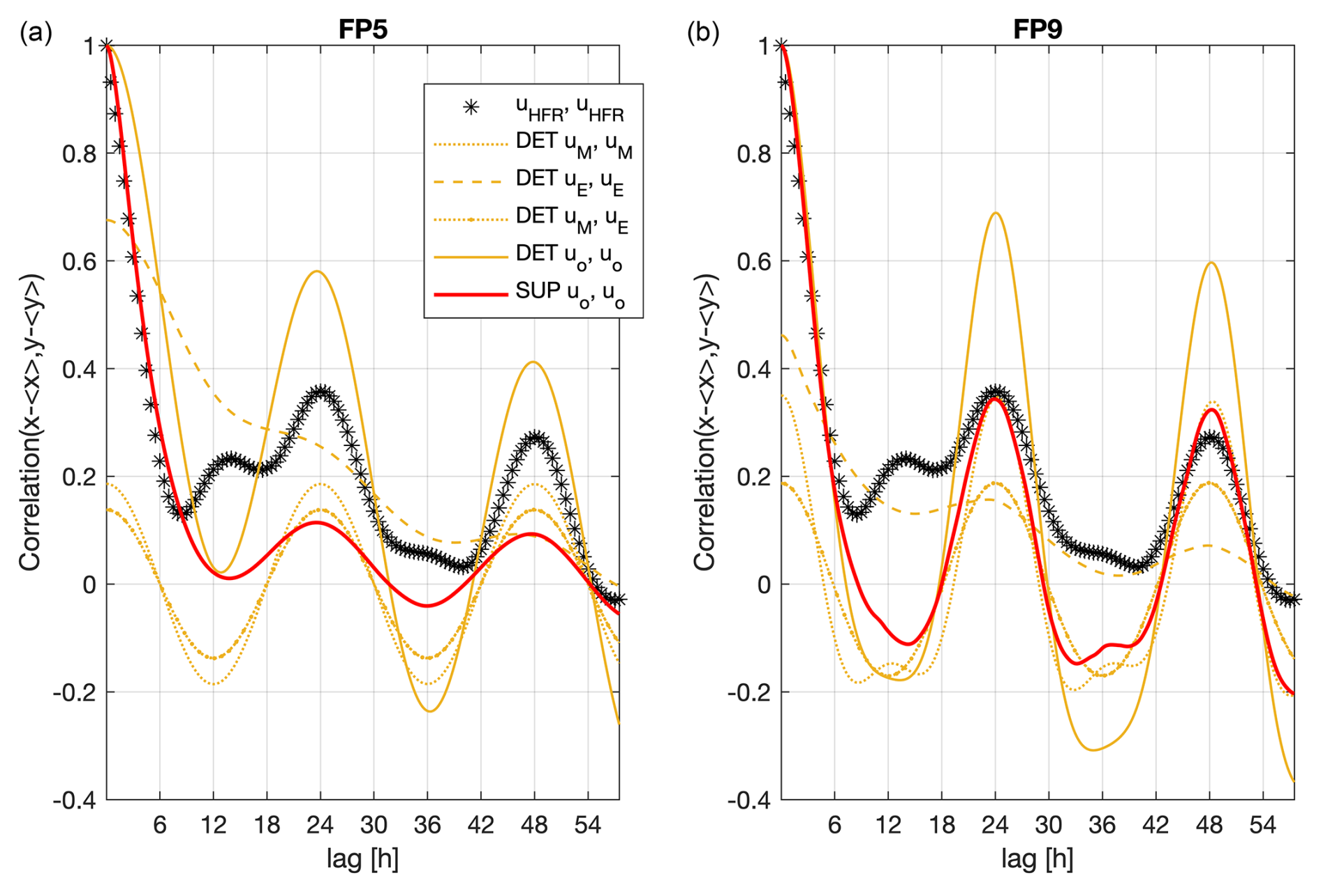
Figure 7 Temporal autocorrelation function of the u component of the HFR sea surface velocities (black asterisks) and of the model variables from FP5 (a) and FP9 (b): autocorrelation of DET u_o (continuous yellow line) and of SUP u_o (continuous red line). The components of the DET u_o autocorrelation are reported: the autocorrelation of DET u_M (yellow dotted line) and of DET u_E (yellow dashed line), and the cross-correlation of DET u_M and u_E (yellow dotted line with dots), where the normalization is based on the DET u_o autocorrelation.

Regarding the deterministic DET model u_o temporal autocorrelation functions shown in Fig. 7, the periodicity of the peaks are consistent with what is observed from the HFR data, while the amplitude of the peaks is higher with respect to the observations. This fact is mainly due to the high autocorrelation of the tidal signal and the absence of stochastic variability. The cross-correlation between the DET u_M and the DET u_E velocities shows a clear undamped periodicity of 1 d. This is due to the daily update of the forecast wind data set: it introduces a spurious artificial periodicity that perfectly correlates with the daily S1-component tidal variability. The observed temporal decay (with a correlation timescale of approximately 5 h) is well reproduced by the DET model u_o autocorrelation from FP9, while it is overestimated by FP5. This can be easily explained: FP5 has a 12 h forcing timescale that brings spurious memory to the system.

The time decay and the modulation of the SUP u_o and v_o temporal autocorrelation functions are well reproduced in both simulations. The fact that the SUP initial decay is comparable with the HFR pattern shows that the value of the γ_u coefficient shown in Table 4 is well chosen. The amplitudes in FP5 underestimate the observed ones, while in FP9, the daily peaks are present. In both simulations, the SUP autocorrelation is more damped in time with respect to the DET one due to the introduction of the stochasticity, as expected. The long time variability of the correlation functions of the idealized models is not expected to be similar to the observed ones, as the model space domain is zero-dimensional and the equations do not include the dynamics of eddies and other coherent two-dimensional structures.

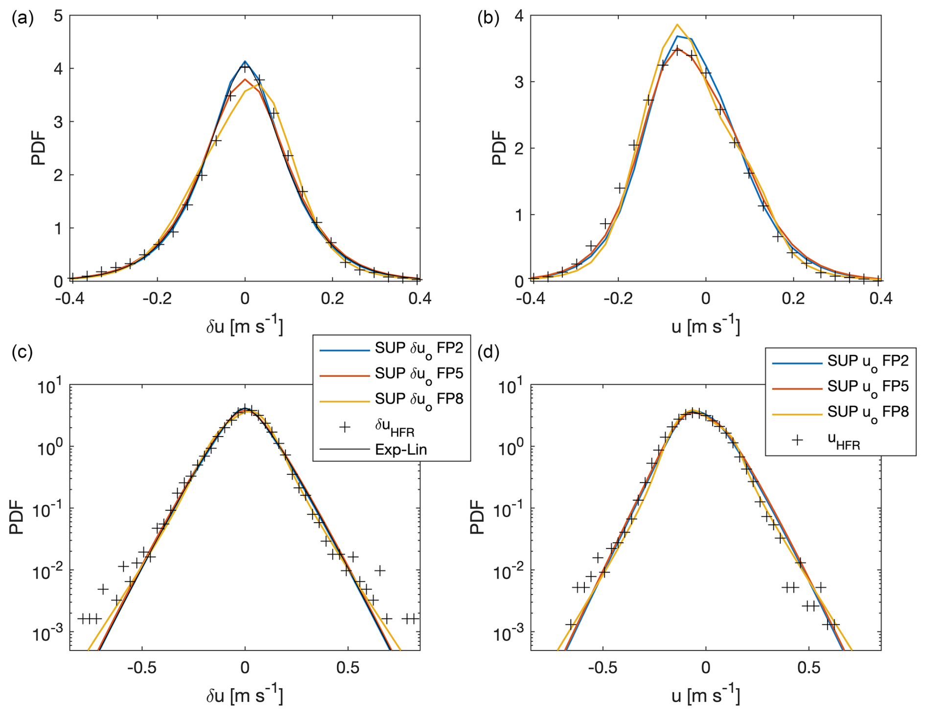
Figure 8 PDFs of the HFR (black crosses) and SUP model total velocity increments δu (a, c) and sea surface velocities u (b, d) in lin–lin plots (a, b) and log–lin plots (c, d) from FP2 (blue line), FP5 (orange line) and FP8 (yellow line). The analytical superstatistical PDF from Eq. (6) is also reported (black line).

We have seen that when moving from longer-forcing-time-averaging FP5 to no-forcing-averaging FP9, the stochastic model needs fewer DOFs. In particular, the number of stochastic DOFs must decrease when the non-averaged tidal components are considered, as reported in Table 2. This can be seen numerically in Fig. 8, where all the PDFs are able to fit the observations appropriately. The rest of the FPs presented in Table 2 (FP3, FP4, FP6 and FP7) are not shown because of the following reasons. FP4 and FP7 do not take into account any wind forcing, so they are not able to mimic the observed velocities. FP3 and FP6, looking at the PDFs of SUP δu_o and u_o, give very similar results to FP5, with the main differences occurring in the height of the PDF peaks.

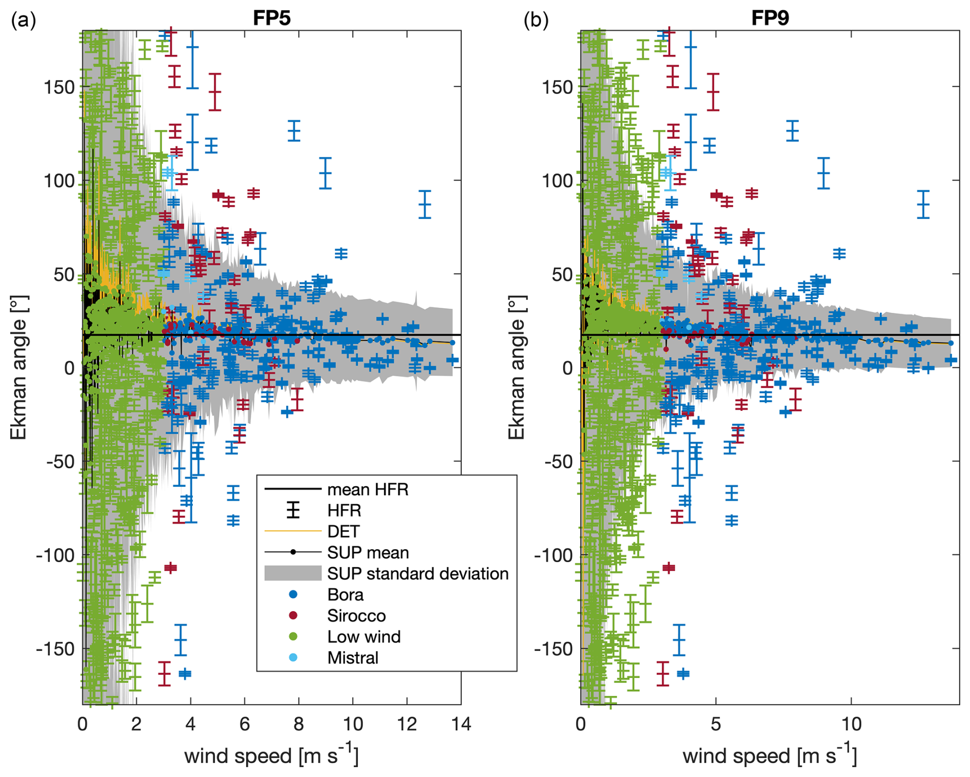
Figure 9 Ekman angle as a function of the daily WRF wind speed using the HFR (sticks with error bars) and the model sea surface currents from FP5 (a) and FP9 (b): DET model Ekman angle (yellow line) and SUP model ensemble mean Ekman angle (black line with coloured dots; the colours indicate the present wind regime). The grey area indicates the SUP model ensemble standard deviation for the Ekman angle. The errors are calculated as shown in Appendix D. The horizontal black line is the observed HFR Ekman angle average.

In order to check if the models capture the observed veering angle, the angle between the daily averaged wind and the daily averaged selected sea surface current is computed (a positive Ekman angle means that the sea surface current is on the right with respect to the wind). As seen in Fig. 9, the observed HFR Ekman angle shows a large spread for low wind regimes, while it accumulates around the observed mean value with stronger wind speeds. In both simulations, the Ekman angle obtained from the DET model (yellow line) collapses towards the same angle range for high wind speeds but with less variability with respect to the observations. The SUP mean Ekman angle is almost the same as for the DET model and converges towards the observed mean Ekman angle with increasing wind speed. The SUP modelled standard deviation (grey area) reflects the observed variability in the entire domain of the Ekman angle for low wind speeds and shows a decrease in variability for stronger wind speeds. The SUP modelled Ekman angle includes, most of the time, the observed Ekman angles inside the 1 standard deviation band. FP5 shows, for both the DET and SUP model, higher variability bands with respect to FP9 due to the higher number of stochastic DOFs.

4.2 The FRR and the SUP model

In this section, the FRR is tested on the SUP model under the forcings of FP9. In Fig. 10, the perturbation methodology on the time series, described in Sect. 3.2, and the effects on the total sea surface velocity are visualized. In this figure, the u_S velocity component is perturbed, while the independent v_S component remains unperturbed. The total SUP u_o velocity component is affected by a clearly visible perturbation that decays in time, while the total SUP v_o velocity component is slightly perturbed through the Ekman drag term.

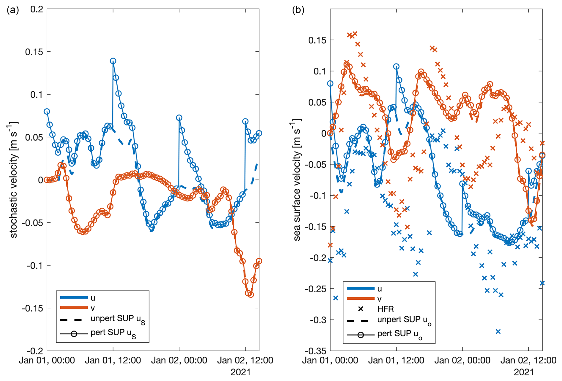
Figure 10 SUP model FP9 stochastic velocities u_S (a). HFR (crosses) and SUP FP9 total sea surface velocities u_o (b). u component is in blue, while v component is in red. The SUP model time series are from the first walker in the unperturbed system (dashed lines) and perturbed system (continuous lines with circles).

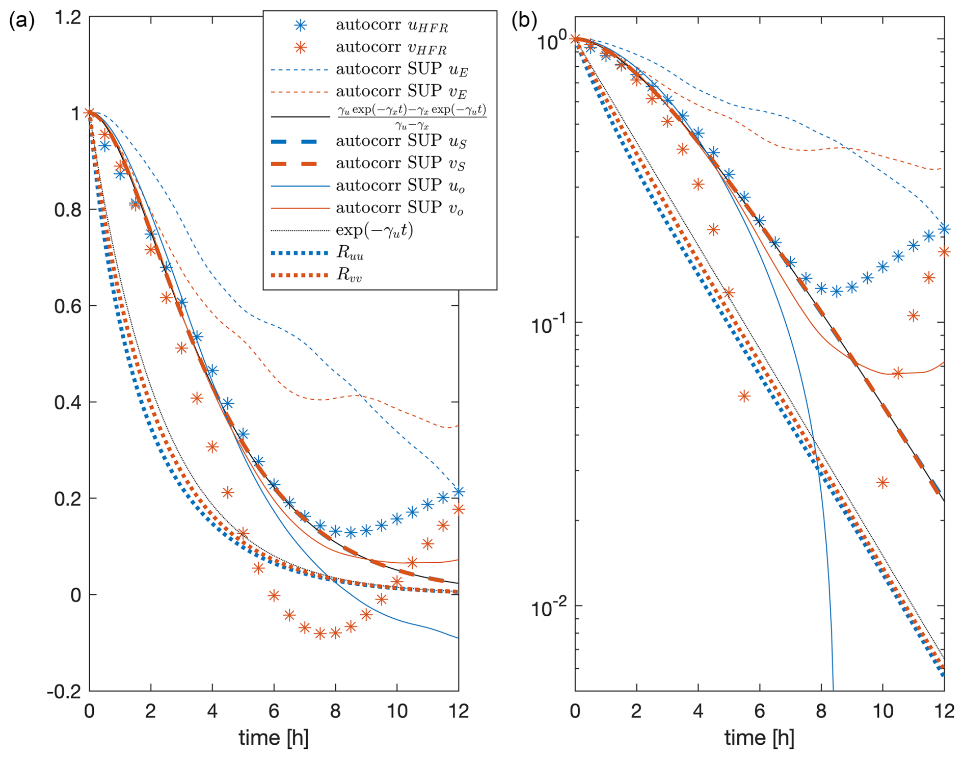
Figure 11 Diagonal response functions (thick dotted lines) and temporal autocorrelations in lin–lin plots (a) and lin–log plots (b) of HFR (asterisks) and unperturbed SUP model FP9 velocities: u_E (dashed and dotted line), u_S (thick dashed line), u_o (continuous line). Blue indicates the u component, while red indicates the v component. The analytical autocorrelation function of the stochastic velocity from Wirth (2019) is reported with the black continuous line. The exponential decay with the stochastic drag coefficient γ_u is shown with the black thin dotted line.

In Fig. 11, the diagonal response functions R_uu(t) and R_vv(t) with the correlations of the observed, unperturbed Ekman, stochastic, and total velocities and analytical functions discussed further are reported. The diagonal response functions show an exponential decay with timescale corresponding to the stochastic velocity drag coefficient γ_u (i.e. $\mathrm{1}/{\mathit{\gamma }}_u\simeq \mathrm{140}$ min; see exponential fit in Fig. 11). When it is u_E or v_E that is perturbed, the diagonal response functions show an exponential decay with timescale corresponding to the mean Ekman drag term $\frac{C_B\stackrel{\mathrm{̃}}{u}}{\stackrel{\mathrm{̃}}{h}}$ (i.e. $\frac{\stackrel{\mathrm{̃}}{h}}{C_B\stackrel{\mathrm{̃}}{u}}\simeq \mathrm{65}$ min; not shown). This reveals that any external perturbation is decaying due to the corresponding model drag (γ_u if we perturb the stochastic velocity; $\frac{C_B\stackrel{\mathrm{̃}}{u}}{\stackrel{\mathrm{̃}}{h}}$ if we perturb the Ekman velocity).

As expected, because u_o and v_o are not Gaussian variables and include terms that are not affected by the perturbation, as the tidal signal, the behaviour of the diagonal response functions differs from the corresponding autocorrelations. It is then not possible to describe the response functions as linear combinations of the correlations in the unperturbed system.

What is particularly interesting to observe in Fig. 11 is that the SUP u_S and v_S autocorrelations coincide with the analytical autocorrelation function for a stochastic Gaussian variable, defined through a linear SDE with coloured Gaussian noise, found by Wirth (2019) in his Appendix C2:

$$\begin{array}{}\text{(15)}& C_{u_{\mathrm{S}}}\left(t\right)={\displaystyle \frac{{\mathit{\gamma }}_u{e}^{-{\mathit{\gamma }}_{x}t}-{\mathit{\gamma }}_x{e}^{-{\mathit{\gamma }}_{u}t}}{{\mathit{\gamma }}_u-{\mathit{\gamma }}_x}},\end{array}$$

showing a dependence on the drag coefficients only and not on the variance of the coloured Gaussian. This result seems surprising, as our stochastic velocities are obtained through a linear SDE with Bessel, not Gaussian, coloured noise. Our interpretation of the fact is the following: the stochastic velocity drag timescale $\mathrm{1}/{\mathit{\gamma }}_u\simeq \mathrm{140}$ min is 1 order of magnitude smaller than the superstatistical Gaussianity timescale T≃2 d of the superstatistical analysis. This means that, under the correlation point of view, the stochastic velocity does not have the time to develop the non-Gaussian characteristics but operates at an almost constant variance. As a consequence, after a decay time of about 5 h, the SUP u_S and v_S autocorrelations collapse exponentially with the same γ_u coefficient of the diagonal response functions. This can also be checked analytically through Eq. (15) and knowing that γ_u<γ_x:

$$\begin{array}{}\text{(16)}& \begin{array}{rl}{C}_{u_{\mathrm{S}}}\left(t\right)& ={\displaystyle \frac{{\mathit{\gamma }}_x}{{\mathit{\gamma }}_u-{\mathit{\gamma }}_x}}\left({\displaystyle \frac{{\mathit{\gamma }}_u}{{\mathit{\gamma }}_x}}{e}^{-{\mathit{\gamma }}_{x}t}-e^{-{\mathit{\gamma }}_{u}t}\right)\\ & \stackrel{t\to \mathrm{\infty }}{⟶}{\displaystyle \frac{{\mathit{\gamma }}_x}{{\mathit{\gamma }}_x-{\mathit{\gamma }}_u}}{e}^{-{\mathit{\gamma }}_{u}t}\propto R_{uu}\left(t\right).\end{array}\end{array}$$

Thus, knowing the autocorrelation function of the stochastic velocity, it is possible to obtain the response function of the total velocity. It is then possible to state that the FRR holds in the SUP model when the perturbation is applied to the stochastic signal.

4.3 Predictability evaluation results

In Fig. 12, the observation-based perturbation methodology on the time series, described in Sect. 3.3, and the effects on the total sea surface velocities are visualized. In this figure, the u_S and v_S velocity components are perturbed. Both the total SUP u_o and v_o show the observation-based perturbation subject to an evident decay in time.

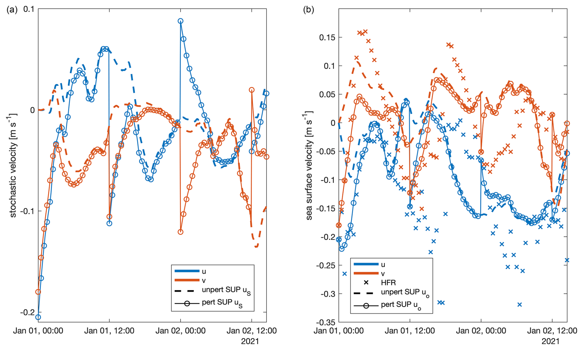
Figure 12 SUP model FP9 stochastic velocities (a), and HFR (crosses) and SUP FP9 total sea surface velocities (b). u component is in blue, and v component is in red. The SUP model time series are from the first walker in the unperturbed system (dashed lines) and perturbed system using a data-assimilation method (continuous lines with circles).

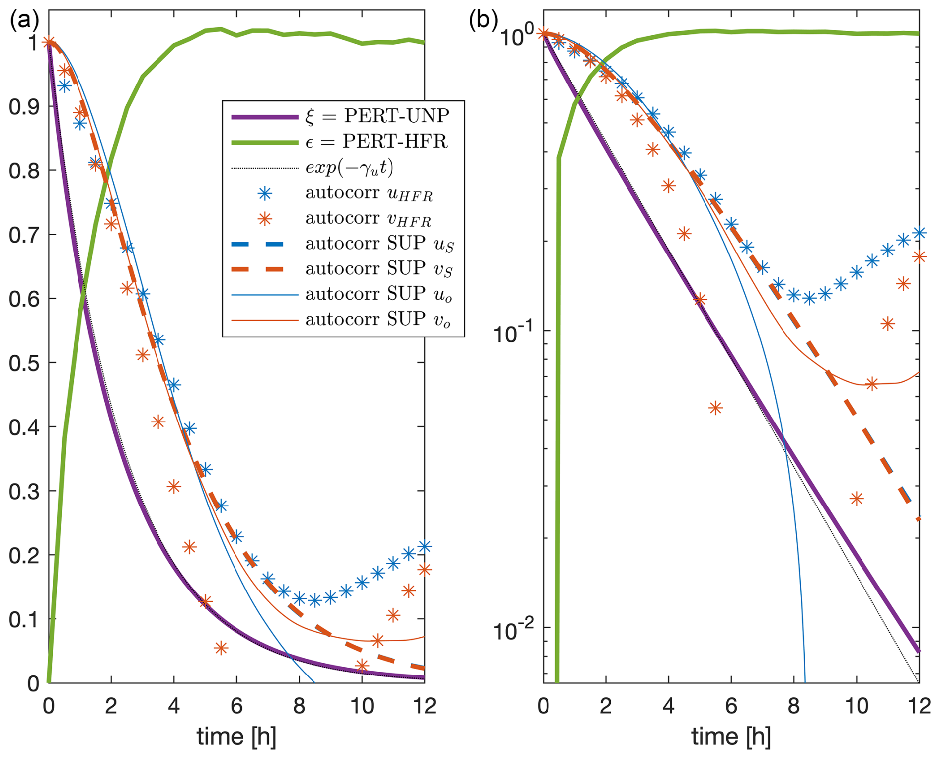
Figure 13 Temporal autocorrelations in lin–lin (a) and lin–log (b) plots of the HFR (asterisks) and SUP model stochastic (thick dashed lines) and total (continuous lines) u (blue) and v (red) sea surface velocities with the ξ (purple thick continuous line) and ϵ (green thick continuous line) functions. The exponential fits of the ξ function are shown (purple thin continuous lines). The exponential decay with the stochastic drag coefficient γ_u is shown by the black thin dotted line.

The ξ(t) and ϵ(t) functions are reported in Fig. 13 and represent the normalized distance between the perturbed–unperturbed and the perturbed–observed systems, respectively. The function ξ(t) can be considered as a generalization of the response function in the FRR when both the components are perturbed of a quantity not known a priori. It is possible to see that the ξ(t) function has an exponential decay with timescale $\mathrm{1}/{\mathit{\gamma }}_u\simeq \mathrm{140}$ min. When the Ekman signal is perturbed, we obtain two exponential decays: τ₁≃75 min for t<2 h and τ₂≃140 min for t>4 h (not shown). The external perturbation, due to the observation-based methodology, decays with the stochastic drag coefficient when we perturb the stochastic velocity, while a clear correspondence with the drag coefficient is not found when the Ekman signal is perturbed. The ϵ(t) function increases its value in time from 0 and, after about 5 h, saturates to 1, showing that, after that time, the perturbed system has completely lost the memory of the initialization to the observations. This time of 5 h coincides with the autocorrelation timescale of the SUP stochastic and total velocities.

5 Conclusions

In the Gulf of Trieste, the analytical superstatistical PDF of the observed HFR sea surface current increments is known (Flora et al., 2023) and is here called Exp-Lin PDF. The Exp-Lin PDF is non-Gaussian with fat tails (the extreme events occur more often with respect to Gaussian statistics), and it provides all the statistical moments but does not give any predictive information. In this study, we have developed a hierarchy of idealized models whose aim is to mimic the sea surface current time series, characterized by the observed statistics.

The hierarchy is organized as follows: the DET model is purely deterministic and includes tidal and Ekman signals, the GAU model adds a coloured-in-time Gaussian stochastic velocity, and the SUP model adds a stochastic sea surface velocity with superstatistical fat-tailed increments that simulate the unresolved dynamics. A variable is superstatistical if it is locally (in time) Gaussian with a variance evolving over a longer timescale. In our case, the variance is obtained through the sum of 2ν squared (Gaussian) Ornstein–Uhlenbeck processes and results to be gamma-distributed. The parameter ν identifies the DOF of the stochastic system. The models are then tested, imposing nine FPs combining different types of tidal and wind forcings: complete, 12 h moving-averaged time series or omitted forcing (Table 2). The stochastic models are adjusted for each FP in order to best fit the observed PDF.

In the following, we point out the general differences between the models' results. The DET model is able to simulate the slow variability of the observed HFR currents, reaching 55 %–56 % of the correlation coefficient (Fig. 4). The GAU and SUP stochastic models increase the variability to observed values, but because their ensemble means almost coincide with the DET model results, they show little influence on the slow dynamics (Fig. 3).

The main differences between the models are evident when looking at the PDFs of their variables. Regarding the total velocity increment PDFs (Fig. 5), the DET model does not explain the variability of the observed superstatistical Exp-Lin PDF, which results in a stark underestimation of the variability. The GAU model improves the results but without the observed fat tails, that is, the occurrence of extreme events is underestimated. When we consider the SUP model, in order to fit the observed statistics, the stochastic modelization requires ν=2 stochastic DOF when the tidal forcing is omitted or averaged, while it needs $\mathit{\nu }=\mathrm{1}/\mathrm{2}$ stochastic DOF when the complete tidal signal is considered (Table 2). This result affects the shape of the SUP stochastic velocity increment PDF (Fig. 2), which is Exp-Lin when ν=2 and Bessel when $\mathit{\nu }=\mathrm{1}/\mathrm{2}$. The SUP model shows a total velocity increment PDF that is representative of observations (Fig. 5): it is almost Exp-Lin when the FP considers averaged forcings and ν=2 stochastic DOF, while it has a shifted and slightly lower peak but tails that satisfactorily fit the observed data when the FP considers the complete forcings and $\mathit{\nu }=\mathrm{1}/\mathrm{2}$ stochastic DOF. The convergence to the PDF and, in particular, the enlargement of the PDF tails to the observed ones in the progression from the DET model to the GAU and then to the SUP model is also visible in the PDFs of the velocities (Fig. 6). In addition, we find that the FP with complete forcings (FP9) and, consequently, with $\mathit{\nu }=\mathrm{1}/\mathrm{2}$ stochastic DOF enables the SUP model to capture the tails with a double slope in the velocity PDF, as seen from the observations.

The velocity temporal autocorrelation functions under FP9 (Fig. 7) reveal that the SUP model, after a realistic time decay of around 5 h (driven by the deterministic signal), allows for a better representation, with respect to the DET model, of the temporal modulations. The Ekman dynamics analysis (Fig. 9) indicates that strong wind increases the likelihood of the SUP model generating trajectories that match the observed average Ekman state. This pattern aligns with the HFR Ekman angle data, where lower wind forcing results in more variability, while higher wind forcing brings values closer to the average.

The SUP model under the most complete forcings and, consequently, with $\mathit{\nu }=\mathrm{1}/\mathrm{2}$ DOF (FP9) is then explored by applying external perturbations to the stochastic signal. The FRR holds when the stochastic signal is perturbed, showing that the response to an external perturbation can be obtained by considering the fluctuations of the unperturbed system. In particular, the SUP model response function decays with the stochastic velocity drag timescale ($\mathrm{1}/{\mathit{\gamma }}_u$; see Fig. 11 and Eq. (16)), indicating a clear memory timescale for external stochastic perturbations.

The predictability evaluation through the observation-based perturbation shows that the SUP model, given any external correction to the HFR values, reaches an equilibrium distance from the observations and converges to the unperturbed realization after 5 h (Fig. 13). This time value is consistent with the autocorrelation decay of the observed and SUP stochastic and total velocities.

From the predictive point of view, we should remark that our modelling is extremely idealized: it is local in space and does not take into account other external forcings besides wind and tides, such as river discharge. The modelling can be further developed by including the Isonzo/Soc̆a river influence, considering other air–sea interaction processes as wave generation, moving the space domain from one point (zero dimensions) to two dimensions by including advection, considering eddy dynamics and incorporating the broader Adriatic circulation.

Despite its idealization, the SUP model presented in this study can reproduce part of the deterministic (tide-wind-forced) large-scale dynamics and the observed fat tails of the HFR velocity increment PDFs and is eventually able to simulate extreme events. One of the most interesting results is that when we have a more detailed deterministic signal (given by the complete forcings), a larger part of the dynamics is resolved, and the stochastic part of the model must not only have less variability but also decrease its DOF. The SUP model can therefore be taken as an example for the modelling community to reflect on how stochasticity can be used to reproduce extreme events and how its characteristics vary depending on the coarse graining of the forcings. Various applications to the SUP model can be found; for example, it is currently used to explore the role of extreme events in the kinetic energy fluxes between the atmosphere and the sea. Additionally, evaluating the air–sea interaction bulk formulas in the CMEMS MFS model (or another full-physics numerical model adopted for the Gulf of Trieste) in light of our observations, and therefore of the SUP model findings, would be extremely interesting.

Appendix A: An analytical idealized case

This is the idealized case of the stochastic system described in Sect. 3, Eqs. (2) and (3), in which

$$\begin{array}{}\text{(A1)}& \sqrt{{\mathrm{\Sigma }}_{i=\mathrm{1}}^{\mathrm{2}\mathit{\nu }}{\mathit{\alpha }}_i^{\mathrm{2}}}=\sqrt{Q}\simeq \text{constant}.\end{array}$$

This approximation and the following analysis make it possible to find the analytical distribution of the variables x, u_S and δu_S. Considering the u components, independent from the v components, Eqs. (2) and (3) can be written as follows:

$$\begin{array}{}\text{(A2)}& \begin{array}{rl}{\displaystyle }& {\displaystyle }\left\{\begin{array}{l}\mathrm{d}x=-{\mathit{\gamma }}_{x}x\mathrm{d}t+\sqrt{Q}\mathrm{d}{W}_x\\ \mathrm{d}{u}_{\mathrm{S}}=-{\mathit{\gamma }}_u{u}_{\mathrm{S}}\mathrm{d}t+\mathit{\eta }x\mathrm{d}t\end{array}\right.\\ {\displaystyle }& {\displaystyle }\begin{array}{rl}{\displaystyle }d\left(\begin{array}{c}x\\ u_{\mathrm{S}}\end{array}\right)& {\displaystyle }=\left(\begin{array}{cc}-{\mathit{\gamma }}_x& \mathrm{0}\\ \mathit{\eta }& -{\mathit{\gamma }}_u\end{array}\right)\left(\begin{array}{c}x\\ u_{\mathrm{S}}\end{array}\right)\mathrm{d}t+\left(\begin{array}{c}\sqrt{Q}\\ \mathrm{0}\end{array}\right)\mathrm{d}{W}_x\\ {\displaystyle }& {\displaystyle }=M\left(\begin{array}{c}x\\ u_{\mathrm{S}}\end{array}\right)\mathrm{d}t+\left(\begin{array}{c}\sqrt{Q}\\ \mathrm{0}\end{array}\right)\mathrm{d}{W}_x,\end{array}\end{array}\end{array}$$

where $M=\left(\begin{array}{cc}-{\mathit{\gamma }}_x& \mathrm{0}\\ \mathit{\eta }& -{\mathit{\gamma }}_u\end{array}\right)$ can be diagonalized:

$$\begin{array}{}\text{(A3)}& \begin{array}{rl}\det (M-mI)& =\det \left(\begin{array}{cc}-{\mathit{\gamma }}_x-m& \mathrm{0}\\ \mathit{\eta }& -{\mathit{\gamma }}_u-m\end{array}\right)\\ & =({\mathit{\gamma }}_x+m)({\mathit{\gamma }}_u+m)=\mathrm{0},\end{array}\end{array}$$

obtaining two eigenvalues $m_{\mathrm{1}}=-{\mathit{\gamma }}_x$ and $m_{\mathrm{2}}=-{\mathit{\gamma }}_u$ and the following eigenvectors (with γ_x≠γ_u):

$$\begin{array}{rl}& M{\mathit{e}}_{\mathrm{1}}=m_{\mathrm{1}}{\mathit{e}}_{\mathrm{1}}\\ & \left(\begin{array}{cc}-{\mathit{\gamma }}_x& \mathrm{0}\\ \mathit{\eta }& -{\mathit{\gamma }}_u\end{array}\right)\left(\begin{array}{c}{e}_{\mathrm{1}x}\\ e_{\mathrm{1}y}\end{array}\right)=-{\mathit{\gamma }}_x\left(\begin{array}{c}{e}_{\mathrm{1}x}\\ e_{\mathrm{1}y}\end{array}\right)\\ & \left\{\begin{array}{l}-{\mathit{\gamma }}_x{e}_{\mathrm{1}x}=-{\mathit{\gamma }}_x{e}_{\mathrm{1}x}\\ \mathit{\eta }{e}_{\mathrm{1}x}-{\mathit{\gamma }}_u{e}_{\mathrm{1}y}=-{\mathit{\gamma }}_x{e}_{\mathrm{1}y}\end{array}\right.\\ & \left\{\begin{array}{l}{e}_{\mathrm{1}y}=-\frac{\mathit{\eta }}{{\mathit{\gamma }}_x-{\mathit{\gamma }}_u}{e}_{\mathrm{1}x}\\ e_{\mathrm{1}x}^{\mathrm{2}}+e_{\mathrm{1}y}^{\mathrm{2}}=\mathrm{1}\end{array}\right.\\ & e_{\mathrm{1}x}^{\mathrm{2}}\left(\mathrm{1}+{\displaystyle \frac{{\mathit{\eta }}^{\mathrm{2}}}{({\mathit{\gamma }}_x-{\mathit{\gamma }}_u{)}^{\mathrm{2}}}}\right)=\mathrm{1}\\ & \left\{\begin{array}{l}{e}_{\mathrm{1}x}=-\frac{{\mathit{\gamma }}_x-{\mathit{\gamma }}_u}{\sqrt{{\mathit{\eta }}^{\mathrm{2}}+({\mathit{\gamma }}_x-{\mathit{\gamma }}_u{)}^{\mathrm{2}}}}\\ e_{\mathrm{1}y}=\frac{\mathit{\eta }}{\sqrt{{\mathit{\eta }}^{\mathrm{2}}+({\mathit{\gamma }}_x-{\mathit{\gamma }}_u{)}^{\mathrm{2}}}}\end{array}\right.\end{array}$$

$$\begin{array}{}\text{(A4)}& {\mathit{e}}_{\mathrm{1}}=\left(\begin{array}{c}-\frac{{\mathit{\gamma }}_x-{\mathit{\gamma }}_u}{\sqrt{{\mathit{\eta }}^{\mathrm{2}}+({\mathit{\gamma }}_x-{\mathit{\gamma }}_u{)}^{\mathrm{2}}}}\\ \frac{\mathit{\eta }}{\sqrt{{\mathit{\eta }}^{\mathrm{2}}+({\mathit{\gamma }}_x-{\mathit{\gamma }}_u{)}^{\mathrm{2}}}}\end{array}\right)\end{array}$$

$$\begin{array}{rl}& M{\mathit{e}}_{\mathrm{2}}=m_{\mathrm{2}}{\mathit{e}}_{\mathrm{2}}\\ & \left(\begin{array}{cc}-{\mathit{\gamma }}_x& \mathrm{0}\\ \mathit{\eta }& -{\mathit{\gamma }}_u\end{array}\right)\left(\begin{array}{c}{e}_{\mathrm{2}x}\\ e_{\mathrm{2}y}\end{array}\right)=-{\mathit{\gamma }}_u\left(\begin{array}{c}{e}_{\mathrm{2}x}\\ e_{\mathrm{2}y}\end{array}\right)\\ & \left\{\begin{array}{l}-{\mathit{\gamma }}_x{e}_{\mathrm{2}x}=-{\mathit{\gamma }}_u{e}_{\mathrm{2}x}\\ \mathit{\eta }{e}_{\mathrm{2}x}-{\mathit{\gamma }}_u{e}_{\mathrm{2}y}=-{\mathit{\gamma }}_u{e}_{\mathrm{2}y}\end{array}\right.\\ & \left\{\begin{array}{l}{e}_{\mathrm{2}x}=\mathrm{0}\\ e_{\mathrm{2}y}=\mathrm{1}\end{array}\right.\end{array}$$

$$\begin{array}{}\text{(A5)}& {\mathit{e}}_{\mathrm{2}}=\left(\begin{array}{c}\mathrm{0}\\ \mathrm{1}\end{array}\right)\end{array}$$

For γ_x≠γ_u, the system in Eq. (A2) is diagonalizable, and it is possible to write $M=T\cdot D\cdot T^{-\mathrm{1}}$, where

$$\begin{array}{}\text{(A6)}& \begin{array}{rl}T& =\left(\begin{array}{cc}-\frac{{\mathit{\gamma }}_x-{\mathit{\gamma }}_u}{\sqrt{{\mathit{\eta }}^{\mathrm{2}}+({\mathit{\gamma }}_x-{\mathit{\gamma }}_u{)}^{\mathrm{2}}}}& \mathrm{0}\\ \frac{\mathit{\eta }}{\sqrt{{\mathit{\eta }}^{\mathrm{2}}+({\mathit{\gamma }}_x-{\mathit{\gamma }}_u{)}^{\mathrm{2}}}}& \mathrm{1}\end{array}\right)D=\left(\begin{array}{cc}-{\mathit{\gamma }}_x& \mathrm{0}\\ \mathrm{0}& -{\mathit{\gamma }}_u\end{array}\right)\\ & T^{-\mathrm{1}}=\left(\begin{array}{cc}-\frac{\sqrt{{\mathit{\eta }}^{\mathrm{2}}+({\mathit{\gamma }}_x-{\mathit{\gamma }}_u{)}^{\mathrm{2}}}}{{\mathit{\gamma }}_x-{\mathit{\gamma }}_u}& \mathrm{0}\\ \frac{\mathit{\eta }}{{\mathit{\gamma }}_x-{\mathit{\gamma }}_u}& \mathrm{1}\end{array}\right).\end{array}\end{array}$$

Thus, hypothesizing that γ_u<γ_x (i.e. the final distributions do not change with γ_x<γ_u; what changes is just the sign of the Wiener processes in the diagonalized system), the following are obtained:

$$\begin{array}{}\text{(A7)}& {\displaystyle }d\left(\begin{array}{c}x\\ u_{\mathrm{S}}\end{array}\right)=T\cdot D\cdot T^{-\mathrm{1}}\left(\begin{array}{c}x\\ u_{\mathrm{S}}\end{array}\right)\mathrm{d}t+\left(\begin{array}{c}\sqrt{Q}\\ \mathrm{0}\end{array}\right)\mathrm{d}{W}_x,\text{(A8)}& {\displaystyle }\begin{array}{rl}d\left[T^{-\mathrm{1}}\left(\begin{array}{c}x\\ u_{\mathrm{S}}\end{array}\right)\right]& =D\left[T^{-\mathrm{1}}\left(\begin{array}{c}x\\ u_{\mathrm{S}}\end{array}\right)\right]\mathrm{d}t\\ & +T^{-\mathrm{1}}\left(\begin{array}{c}\sqrt{Q}\\ \mathrm{0}\end{array}\right)\mathrm{d}{W}_x,\end{array}\text{(A9)}& {\displaystyle }\begin{array}{rl}& \left(\begin{array}{c}\stackrel{\mathrm{̃}}{x}\\ \stackrel{\mathrm{̃}}{u_{\mathrm{S}}}\end{array}\right)=T^{-\mathrm{1}}\left(\begin{array}{c}x\\ u_{\mathrm{S}}\end{array}\right)=\left(\begin{array}{c}-\frac{\sqrt{{\mathit{\eta }}^{\mathrm{2}}+({\mathit{\gamma }}_x-{\mathit{\gamma }}_u{)}^{\mathrm{2}}}}{{\mathit{\gamma }}_x-{\mathit{\gamma }}_u}x\\ u_{\mathrm{S}}+\frac{\mathit{\eta }}{{\mathit{\gamma }}_x-{\mathit{\gamma }}_u}x\end{array}\right),\\ & \left(\begin{array}{c}-\sqrt{Q_x}\\ \sqrt{Q_u}\end{array}\right)=T^{-\mathrm{1}}\left(\begin{array}{c}\sqrt{Q}\\ \mathrm{0}\end{array}\right)\\ & =\left(\begin{array}{c}-\frac{\sqrt{{\mathit{\eta }}^{\mathrm{2}}+({\mathit{\gamma }}_x-{\mathit{\gamma }}_u{)}^{\mathrm{2}}}}{{\mathit{\gamma }}_x-{\mathit{\gamma }}_u}\sqrt{Q}\\ \frac{\mathit{\eta }}{{\mathit{\gamma }}_x-{\mathit{\gamma }}_u}\sqrt{Q}\end{array}\right),\end{array}\end{array}$$

yielding

$$\begin{array}{}\text{(A10)}& \begin{array}{rl}{\displaystyle }& {\displaystyle }d\left(\begin{array}{c}\stackrel{\mathrm{̃}}{x}\\ \stackrel{\mathrm{̃}}{u_{\mathrm{S}}}\end{array}\right)=D\left(\begin{array}{c}\stackrel{\mathrm{̃}}{x}\\ \stackrel{\mathrm{̃}}{u_{\mathrm{S}}}\end{array}\right)\mathrm{d}t+\left(\begin{array}{c}-\sqrt{Q_x}\\ \sqrt{Q_u}\end{array}\right)\mathrm{d}{W}_x\\ {\displaystyle }& {\displaystyle }\left\{\begin{array}{l}\mathrm{d}\stackrel{\mathrm{̃}}{x}=-{\mathit{\gamma }}_x\stackrel{\mathrm{̃}}{x}\mathrm{d}t-\sqrt{Q_x}\mathrm{d}{W}_x\\ \mathrm{d}\stackrel{\mathrm{̃}}{u_{\mathrm{S}}}=-{\mathit{\gamma }}_u\stackrel{\mathrm{̃}}{u_{\mathrm{S}}}\mathrm{d}t+\sqrt{Q_u}\mathrm{d}{W}_x\end{array}\right..\end{array}\end{array}$$

The approximation for which $\sqrt{Q}=\text{constant}$ leads to $\sqrt{Q_x}$ and $\sqrt{Q_u}$ also being constants. This fact leads to the Gaussianity of the variables $\stackrel{\mathrm{̃}}{x}$ and $\stackrel{\mathrm{̃}}{u_{\mathrm{S}}}$ (they are Ornstein–Uhlenbeck processes):

$$\begin{array}{}\text{(A11)}& \left\{\begin{array}{l}\stackrel{\mathrm{̃}}{x}\sim N\left(\mathrm{0},{\mathit{\sigma }}_{\stackrel{\mathrm{̃}}{x}}^{\mathrm{2}}\right)=N\left(\mathrm{0},\frac{Q_x}{\mathrm{2}{\mathit{\gamma }}_x}\right)=N\left(\mathrm{0},\frac{{\mathit{\eta }}^{\mathrm{2}}+({\mathit{\gamma }}_x-{\mathit{\gamma }}_u{)}^{\mathrm{2}}}{({\mathit{\gamma }}_x-{\mathit{\gamma }}_u{)}^{\mathrm{2}}}\frac{Q}{\mathrm{2}{\mathit{\gamma }}_x}\right)\\ \stackrel{\mathrm{̃}}{u_{\mathrm{S}}}\sim N\left(\mathrm{0},{\mathit{\sigma }}_{\stackrel{\mathrm{̃}}{u_{\mathrm{S}}}}^{\mathrm{2}}\right)=N\left(\mathrm{0},\frac{Q_u}{\mathrm{2}{\mathit{\gamma }}_u}\right)=N\left(\mathrm{0},\frac{{\mathit{\eta }}^{\mathrm{2}}}{({\mathit{\gamma }}_x-{\mathit{\gamma }}_u{)}^{\mathrm{2}}}\frac{Q}{\mathrm{2}{\mathit{\gamma }}_u}\right)\end{array}\right..\end{array}$$

From Eq. (A9), it is possible to write x and u_S in terms of $\stackrel{\mathrm{̃}}{x}$ and $\stackrel{\mathrm{̃}}{u_{\mathrm{S}}}$, resulting in linear combinations of Gaussian variables:

$$\begin{array}{}\text{(A12)}& \left\{\begin{array}{l}x=-\frac{{\mathit{\gamma }}_x-{\mathit{\gamma }}_u}{\sqrt{{\mathit{\eta }}^{\mathrm{2}}+({\mathit{\gamma }}_x-{\mathit{\gamma }}_u{)}^{\mathrm{2}}}}\stackrel{\mathrm{̃}}{x}\\ u_{\mathrm{S}}=\stackrel{\mathrm{̃}}{u_{\mathrm{S}}}+\stackrel{\mathrm{̃}}{r}\\ \stackrel{\mathrm{̃}}{r}=-\frac{\mathit{\eta }}{{\mathit{\gamma }}_x-{\mathit{\gamma }}_u}x=\frac{\mathit{\eta }}{\sqrt{{\mathit{\eta }}^{\mathrm{2}}+({\mathit{\gamma }}_x-{\mathit{\gamma }}_u{)}^{\mathrm{2}}}}\stackrel{\mathrm{̃}}{x}\end{array}\right..\end{array}$$

This leads to the Gaussianity of the variables x, $\stackrel{\mathrm{̃}}{r}$ and u_S with the following variances:

$$\begin{array}{}\text{(A13)}& {\displaystyle }\left\{\begin{array}{l}x\sim N\left(\mathrm{0},{\mathit{\sigma }}_x^{\mathrm{2}}\right)\\ \stackrel{\mathrm{̃}}{r}\sim N\left(\mathrm{0},{\mathit{\sigma }}_{\stackrel{\mathrm{̃}}{r}}^{\mathrm{2}}\right)\\ u_{\mathrm{S}}\sim N\left(\mathrm{0},{\mathit{\sigma }}_{u_{\mathrm{S}}}^{\mathrm{2}}\right)\end{array}\right.,\text{(A14)}& {\displaystyle }\left\{\begin{array}{ll}{\mathit{\sigma }}_x^{\mathrm{2}}& =\frac{({\mathit{\gamma }}_x-{\mathit{\gamma }}_u{)}^{\mathrm{2}}}{{\mathit{\eta }}^{\mathrm{2}}+({\mathit{\gamma }}_x-{\mathit{\gamma }}_u{)}^{\mathrm{2}}}{\mathit{\sigma }}_{\stackrel{\mathrm{̃}}{x}}^{\mathrm{2}}=\frac{Q}{\mathrm{2}{\mathit{\gamma }}_x}\\ {\mathit{\sigma }}_{\stackrel{\mathrm{̃}}{r}}^{\mathrm{2}}& =\frac{{\mathit{\eta }}^{\mathrm{2}}}{{\mathit{\eta }}^{\mathrm{2}}+({\mathit{\gamma }}_x-{\mathit{\gamma }}_u{)}^{\mathrm{2}}}{\mathit{\sigma }}_{\stackrel{\mathrm{̃}}{x}}^{\mathrm{2}}=\frac{{\mathit{\eta }}^{\mathrm{2}}}{({\mathit{\gamma }}_x-{\mathit{\gamma }}_u{)}^{\mathrm{2}}}\frac{Q}{\mathrm{2}{\mathit{\gamma }}_x}\\ {\mathit{\sigma }}_{u_{\mathrm{S}}}^{\mathrm{2}}& ={\mathit{\sigma }}_{\stackrel{\mathrm{̃}}{u_{\mathrm{S}}}}^{\mathrm{2}}+{\mathit{\sigma }}_{\stackrel{\mathrm{̃}}{r}}^{\mathrm{2}}+\mathrm{2}{lim}_{t\to \mathrm{\infty }}\text{corr}\left(\stackrel{\mathrm{̃}}{u_{\mathrm{S}}}\right(t),\stackrel{\mathrm{̃}}{r}(t\left)\right)\\ & =\frac{{\mathit{\eta }}^{\mathrm{2}}}{({\mathit{\gamma }}_x-{\mathit{\gamma }}_u{)}^{\mathrm{2}}}\frac{Q}{\mathrm{2}{\mathit{\gamma }}_u}+\frac{{\mathit{\eta }}^{\mathrm{2}}}{({\mathit{\gamma }}_x-{\mathit{\gamma }}_u{)}^{\mathrm{2}}}\frac{Q}{\mathrm{2}{\mathit{\gamma }}_x}\\ & +\mathrm{2}\frac{\mathit{\eta }}{\sqrt{{\mathit{\eta }}^{\mathrm{2}}+({\mathit{\gamma }}_x-{\mathit{\gamma }}_u{)}^{\mathrm{2}}}}{lim}_{t\to \mathrm{\infty }}\text{corr}\left(\stackrel{\mathrm{̃}}{u_{\mathrm{S}}}\right(t),\stackrel{\mathrm{̃}}{x}(t\left)\right)\\ & =\frac{{\mathit{\eta }}^{\mathrm{2}}({\mathit{\gamma }}_x+{\mathit{\gamma }}_u)}{({\mathit{\gamma }}_x-{\mathit{\gamma }}_u{)}^{\mathrm{2}}}\frac{Q}{\mathrm{2}{\mathit{\gamma }}_x{\mathit{\gamma }}_u}-\frac{\mathrm{2}{\mathit{\eta }}^{\mathrm{2}}}{({\mathit{\gamma }}_x-{\mathit{\gamma }}_u{)}^{\mathrm{2}}({\mathit{\gamma }}_x+{\mathit{\gamma }}_u)}Q\\ & =\frac{{\mathit{\eta }}^{\mathrm{2}}}{({\mathit{\gamma }}_x-{\mathit{\gamma }}_u{)}^{\mathrm{2}}}\frac{({\mathit{\gamma }}_x+{\mathit{\gamma }}_u{)}^{\mathrm{2}}-\mathrm{4}{\mathit{\gamma }}_x{\mathit{\gamma }}_u}{\mathrm{2}{\mathit{\gamma }}_x{\mathit{\gamma }}_u({\mathit{\gamma }}_x+{\mathit{\gamma }}_u)}Q\\ & =\frac{{\mathit{\eta }}^{\mathrm{2}}}{\mathrm{2}{\mathit{\gamma }}_x{\mathit{\gamma }}_u({\mathit{\gamma }}_x+{\mathit{\gamma }}_u)}Q\end{array}\right.,\end{array}$$

where, because $\stackrel{\mathrm{̃}}{x}$ and $\stackrel{\mathrm{̃}}{u_{\mathrm{S}}}$ are Ornstein–Uhlenbeck processes:

$$\begin{array}{}\text{(A15)}& \left\{\begin{array}{l}\stackrel{\mathrm{̃}}{x}\left(t\right)=-e^{-{\mathit{\gamma }}_{x}t}{\int }_{\mathrm{0}}^t{e}^{{\mathit{\gamma }}_x{t}^{\prime }}\sqrt{Q_x}F\left(t^{\prime }\right)\mathrm{d}{t}^{\prime }\\ \stackrel{\mathrm{̃}}{u_{\mathrm{S}}}\left(t\right)=e^{-{\mathit{\gamma }}_{u}t}{\int }_{\mathrm{0}}^t{e}^{{\mathit{\gamma }}_u{t}^{\prime }}\sqrt{Q_u}F\left(t^{\prime }\right)\mathrm{d}{t}^{\prime }\\ E\left[F\right(t^{\prime }\left)F\right(t^{\prime \prime }\left)\right]=\mathit{\delta }(t^{\prime }-t^{\prime \prime })\end{array}\right.,\end{array}$$

we have that

$$\begin{array}{}\text{(A16)}& \begin{array}{rl}\text{corr}& \left(\stackrel{\mathrm{̃}}{u_{\mathrm{S}}}\right(t),\stackrel{\mathrm{̃}}{x}(t\left)\right)=-e^{-({\mathit{\gamma }}_x+{\mathit{\gamma }}_u)t}\\ & \sqrt{Q_x{Q}_u}\underset{\mathrm{0}}{\overset{t}{\int }}\underset{\mathrm{0}}{\overset{t}{\int }}{e}^{{\mathit{\gamma }}_x{t}^{\prime }}{e}^{{\mathit{\gamma }}_u{t}^{\prime \prime }}E\left[F\right(t^{\prime }\left)F\right(t^{\prime \prime }\left)\right]\mathrm{d}{t}^{\prime }\mathrm{d}{t}^{\prime \prime }\\ & =-{\displaystyle \frac{\mathit{\eta }\sqrt{{\mathit{\eta }}^{\mathrm{2}}+({\mathit{\gamma }}_x-{\mathit{\gamma }}_u{)}^{\mathrm{2}}}}{({\mathit{\gamma }}_x-{\mathit{\gamma }}_u{)}^{\mathrm{2}}}}Q{e}^{-({\mathit{\gamma }}_x+{\mathit{\gamma }}_u)t}{\displaystyle \frac{e^{({\mathit{\gamma }}_x+{\mathit{\gamma }}_u)t}-\mathrm{1}}{{\mathit{\gamma }}_x+{\mathit{\gamma }}_u}}\\ & =-{\displaystyle \frac{\mathit{\eta }\sqrt{{\mathit{\eta }}^{\mathrm{2}}+({\mathit{\gamma }}_x-{\mathit{\gamma }}_u{)}^{\mathrm{2}}}}{({\mathit{\gamma }}_x-{\mathit{\gamma }}_u{)}^{\mathrm{2}}}}{\displaystyle \frac{Q}{{\mathit{\gamma }}_x+{\mathit{\gamma }}_u}}\left(\mathrm{1}-e^{-({\mathit{\gamma }}_x+{\mathit{\gamma }}_u)t}\right)\\ & \stackrel{t\to \mathrm{\infty }}{⟶}-{\displaystyle \frac{\mathit{\eta }\sqrt{{\mathit{\eta }}^{\mathrm{2}}+({\mathit{\gamma }}_x-{\mathit{\gamma }}_u{)}^{\mathrm{2}}}}{({\mathit{\gamma }}_x-{\mathit{\gamma }}_u{)}^{\mathrm{2}}}}{\displaystyle \frac{Q}{{\mathit{\gamma }}_x+{\mathit{\gamma }}_u}}.\end{array}\end{array}$$

Now, it is possible to express the δu_S variable, starting from its definition and using Eq. (A14), in terms of the diagonalized variables $\stackrel{\mathrm{̃}}{x}$ and $\stackrel{\mathrm{̃}}{u_{\mathrm{S}}}$:

$$\begin{array}{}\text{(A17)}& \begin{array}{rl}\mathit{\delta }{u}_{\mathrm{S}}\left(t\right)& =u_{\mathrm{S}}(t+\mathit{\delta })-u_{\mathrm{S}}\left(t\right)\\ & =\stackrel{\mathrm{̃}}{u_{\mathrm{S}}}(t+\mathit{\delta })+{\displaystyle \frac{\mathit{\eta }}{\sqrt{{\mathit{\eta }}^{\mathrm{2}}+{\left({\mathit{\gamma }}_x-{\mathit{\gamma }}_u\right)}^{\mathrm{2}}}}}\\ & \stackrel{\mathrm{̃}}{x}(t+\mathit{\delta })-\stackrel{\mathrm{̃}}{u_{\mathrm{S}}}\left(t\right)-{\displaystyle \frac{\mathit{\eta }}{\sqrt{{\mathit{\eta }}^{\mathrm{2}}+{\left({\mathit{\gamma }}_x-{\mathit{\gamma }}_u\right)}^{\mathrm{2}}}}}\stackrel{\mathrm{̃}}{x}\left(t\right)\\ & =\left[\stackrel{\mathrm{̃}}{u_{\mathrm{S}}}(t+\mathit{\delta })-\stackrel{\mathrm{̃}}{u_{\mathrm{S}}}\left(t\right)\right]\\ & +{\displaystyle \frac{\mathit{\eta }}{\sqrt{{\mathit{\eta }}^{\mathrm{2}}+{\left({\mathit{\gamma }}_x-{\mathit{\gamma }}_u\right)}^{\mathrm{2}}}}}\left[\stackrel{\mathrm{̃}}{x}(t+\mathit{\delta })-\stackrel{\mathrm{̃}}{x}\left(t\right)\right]\\ & =\stackrel{\mathrm{̃}}{\mathit{\delta }{u}_{\mathrm{S}}}\left(t\right)+{\displaystyle \frac{\mathit{\eta }}{\sqrt{{\mathit{\eta }}^{\mathrm{2}}+{\left({\mathit{\gamma }}_x-{\mathit{\gamma }}_u\right)}^{\mathrm{2}}}}}\stackrel{\mathrm{̃}}{\mathit{\delta }x}\left(t\right),\end{array}\end{array}$$

where

$$\begin{array}{}\text{(A18)}& \left\{\begin{array}{l}\stackrel{\mathrm{̃}}{\mathit{\delta }{u}_{\mathrm{S}}}\left(t\right)=\stackrel{\mathrm{̃}}{u_{\mathrm{S}}}(t+\mathit{\delta })-\stackrel{\mathrm{̃}}{u_{\mathrm{S}}}\left(t\right)\\ \stackrel{\mathrm{̃}}{\mathit{\delta }x}\left(t\right)=\stackrel{\mathrm{̃}}{x}(t+\mathit{\delta })-\stackrel{\mathrm{̃}}{x}\left(t\right)\end{array}\right..\end{array}$$

Because $\stackrel{\mathrm{̃}}{\mathit{\delta }{u}_{\mathrm{S}}}$ and $\stackrel{\mathrm{̃}}{\mathit{\delta }x}$ are linear combinations of Gaussian variables, they are Gaussian variables themselves:

$$\begin{array}{}\text{(A19)}& \left\{\begin{array}{l}\stackrel{\mathrm{̃}}{\mathit{\delta }{u}_{\mathrm{S}}}\sim N(\mathrm{0},{\mathit{\sigma }}_{\stackrel{\mathrm{̃}}{\mathit{\delta }{u}_{\mathrm{S}}}}^{\mathrm{2}})\\ \begin{array}{rl}{\displaystyle }{\mathit{\sigma }}_{\stackrel{\mathrm{̃}}{\mathit{\delta }{u}_{\mathrm{S}}}}^{\mathrm{2}}& {\displaystyle }=\mathrm{2}{\mathit{\sigma }}_{\stackrel{\mathrm{̃}}{u_{\mathrm{S}}}}^{\mathrm{2}}+\mathrm{2}\underset{t\to \mathrm{\infty }}{lim}\text{corr}\left(\stackrel{\mathrm{̃}}{u_{\mathrm{S}}}(t+\mathit{\delta }),\stackrel{\mathrm{̃}}{u_{\mathrm{S}}}\left(t\right)\right)\\ {\displaystyle }& {\displaystyle }=\mathrm{2}{\displaystyle \frac{{\mathit{\eta }}^{\mathrm{2}}}{{\left({\mathit{\gamma }}_x-{\mathit{\gamma }}_u\right)}^{\mathrm{2}}}}{\displaystyle \frac{Q}{\mathrm{2}{\mathit{\gamma }}_u}}\left(\mathrm{1}-e^{-{\mathit{\gamma }}_u\mathit{\delta }}\right)\end{array}\\ \stackrel{\mathrm{̃}}{\mathit{\delta }x}\sim N(\mathrm{0},{\mathit{\sigma }}_{\stackrel{\mathrm{̃}}{\mathit{\delta }x}}^{\mathrm{2}})\\ \begin{array}{rl}{\displaystyle }{\mathit{\sigma }}_{\stackrel{\mathrm{̃}}{\mathit{\delta }x}}^{\mathrm{2}}& {\displaystyle }=\mathrm{2}{\mathit{\sigma }}_{\stackrel{\mathrm{̃}}{x}}^{\mathrm{2}}+\mathrm{2}\underset{t\to \mathrm{\infty }}{lim}\text{corr}\left(\stackrel{\mathrm{̃}}{x}(t+\mathit{\delta }),\stackrel{\mathrm{̃}}{x}\left(t\right)\right)\\ {\displaystyle }& {\displaystyle }=\mathrm{2}{\displaystyle \frac{{\mathit{\eta }}^{\mathrm{2}}+{\left({\mathit{\gamma }}_x-{\mathit{\gamma }}_u\right)}^{\mathrm{2}}}{{\left({\mathit{\gamma }}_x-{\mathit{\gamma }}_u\right)}^{\mathrm{2}}}}{\displaystyle \frac{Q}{\mathrm{2}{\mathit{\gamma }}_x}}\left(\mathrm{1}-e^{-{\mathit{\gamma }}_x\mathit{\delta }}\right)\end{array}\end{array}\right.,\end{array}$$

where

$$\begin{array}{}\text{(A20)}& \begin{array}{rl}\text{corr}& \left(\stackrel{\mathrm{̃}}{u_{\mathrm{S}}}(t+\mathit{\delta }),\stackrel{\mathrm{̃}}{u_{\mathrm{S}}}\left(t\right)\right)={\displaystyle \frac{{\mathit{\eta }}^{\mathrm{2}}Q}{{\left({\mathit{\gamma }}_x-{\mathit{\gamma }}_u\right)}^{\mathrm{2}}}}\\ & e^{-\mathrm{2}{\mathit{\gamma }}_{u}t}{e}^{-{\mathit{\gamma }}_u\mathit{\delta }}\underset{\mathrm{0}}{\overset{t+\mathit{\delta }}{\int }}\underset{\mathrm{0}}{\overset{t}{\int }}{e}^{{\mathit{\gamma }}_u{t}^{\prime }}{e}^{{\mathit{\gamma }}_u{t}^{\prime \prime }}\mathit{\delta }\left(t^{\prime }-t^{\prime \prime }\right)\mathrm{d}{t}^{\prime }\mathrm{d}{t}^{\prime \prime }\\ & ={\displaystyle \frac{{\mathit{\eta }}^{\mathrm{2}}Q}{{\left({\mathit{\gamma }}_x-{\mathit{\gamma }}_u\right)}^{\mathrm{2}}}}{e}^{-\mathrm{2}{\mathit{\gamma }}_{u}t}{e}^{-{\mathit{\gamma }}_u\mathit{\delta }}\underset{\mathrm{0}}{\overset{t}{\int }}{e}^{\mathrm{2}{\mathit{\gamma }}_u{t}^{\prime }}\mathrm{d}{t}^{\prime }\\ & ={\displaystyle \frac{{\mathit{\eta }}^{\mathrm{2}}Q}{{\left({\mathit{\gamma }}_x-{\mathit{\gamma }}_u\right)}^{\mathrm{2}}}}{e}^{-{\mathit{\gamma }}_u\mathit{\delta }}{e}^{-\mathrm{2}{\mathit{\gamma }}_{u}t}{\displaystyle \frac{e^{\mathrm{2}{\mathit{\gamma }}_{u}t}-\mathrm{1}}{\mathrm{2}{\mathit{\gamma }}_u}}\\ & ={\displaystyle \frac{{\mathit{\eta }}^{\mathrm{2}}Q}{{\left({\mathit{\gamma }}_x-{\mathit{\gamma }}_u\right)}^{\mathrm{2}}}}{\displaystyle \frac{e^{-{\mathit{\gamma }}_u\mathit{\delta }}}{\mathrm{2}{\mathit{\gamma }}_u}}\left(\mathrm{1}-e^{-\mathrm{2}{\mathit{\gamma }}_{u}t}\right)\\ & \stackrel{t\to \mathrm{\infty }}{⟶}{\displaystyle \frac{{\mathit{\eta }}^{\mathrm{2}}}{{\left({\mathit{\gamma }}_x-{\mathit{\gamma }}_u\right)}^{\mathrm{2}}}}{\displaystyle \frac{Q}{\mathrm{2}{\mathit{\gamma }}_u}}{e}^{-{\mathit{\gamma }}_u\mathit{\delta }},\end{array}\end{array}$$

$$\begin{array}{}\text{(A21)}& \begin{array}{rl}\text{corr}& \left(\stackrel{\mathrm{̃}}{x}(t+\mathit{\delta }),\stackrel{\mathrm{̃}}{x}\left(t\right)\right)={\displaystyle \frac{{\mathit{\eta }}^{\mathrm{2}}+{\left({\mathit{\gamma }}_x-{\mathit{\gamma }}_u\right)}^{\mathrm{2}}}{{\left({\mathit{\gamma }}_x-{\mathit{\gamma }}_u\right)}^{\mathrm{2}}}}\\ & Q{e}^{-\mathrm{2}{\mathit{\gamma }}_{x}t}{e}^{-{\mathit{\gamma }}_x\mathit{\delta }}\underset{\mathrm{0}}{\overset{t+\mathit{\delta }}{\int }}\underset{\mathrm{0}}{\overset{t}{\int }}{e}^{{\mathit{\gamma }}_x{t}^{\prime }}{e}^{{\mathit{\gamma }}_x{t}^{\prime \prime }}\mathit{\delta }\left(t^{\prime }-t^{\prime \prime }\right)\mathrm{d}{t}^{\prime }\mathrm{d}{t}^{\prime \prime }\\ & ={\displaystyle \frac{{\mathit{\eta }}^{\mathrm{2}}+{\left({\mathit{\gamma }}_x-{\mathit{\gamma }}_u\right)}^{\mathrm{2}}}{{\left({\mathit{\gamma }}_x-{\mathit{\gamma }}_u\right)}^{\mathrm{2}}}}Q{e}^{-\mathrm{2}{\mathit{\gamma }}_{x}t}{e}^{-{\mathit{\gamma }}_x\mathit{\delta }}\underset{\mathrm{0}}{\overset{t}{\int }}{e}^{\mathrm{2}{\mathit{\gamma }}_x{t}^{\prime }}\mathrm{d}{t}^{\prime }\\ & ={\displaystyle \frac{{\mathit{\eta }}^{+}{\left({\mathit{\gamma }}_x-{\mathit{\gamma }}_u\right)}^{\mathrm{2}}}{{\left({\mathit{\gamma }}_x-{\mathit{\gamma }}_u\right)}^{\mathrm{2}}}}Q{e}^{-{\mathit{\gamma }}_x\mathit{\delta }}{e}^{-\mathrm{2}{\mathit{\gamma }}_{x}t}{\displaystyle \frac{e^{\mathrm{2}{\mathit{\gamma }}_{x}t}-\mathrm{1}}{\mathrm{2}{\mathit{\gamma }}_x}}\\ & ={\displaystyle \frac{{\mathit{\eta }}^{\mathrm{2}}+{\left({\mathit{\gamma }}_x-{\mathit{\gamma }}_u\right)}^{\mathrm{2}}}{{\left({\mathit{\gamma }}_x-{\mathit{\gamma }}_u\right)}^{\mathrm{2}}}}{\displaystyle \frac{Q}{\mathrm{2}{\mathit{\gamma }}_x}}{e}^{-{\mathit{\gamma }}_x\mathit{\delta }}\left(\mathrm{1}-e^{-\mathrm{2}{\mathit{\gamma }}_{x}t}\right)\\ & \stackrel{t\to \mathrm{\infty }}{⟶}{\displaystyle \frac{{\mathit{\eta }}^{\mathrm{2}}+{\left({\mathit{\gamma }}_x-{\mathit{\gamma }}_u\right)}^{\mathrm{2}}}{{\left({\mathit{\gamma }}_x-{\mathit{\gamma }}_u\right)}^{\mathrm{2}}}}{\displaystyle \frac{Q}{\mathrm{2}{\mathit{\gamma }}_x}}{e}^{-{\mathit{\gamma }}_x\mathit{\delta }}.\end{array}\end{array}$$

Now, according to Eqs. (A17) and (A19), because δu_S is a linear combination of Gaussian variables, it is Gaussian-distributed itself:

$$\begin{array}{}\text{(A22)}& \left\{\begin{array}{l}\mathit{\delta }{u}_{\mathrm{S}}\sim N(\mathrm{0},{\mathit{\sigma }}_{\mathit{\delta }u}^{\mathrm{2}})\\ {\mathit{\sigma }}_{\mathit{\delta }u}^{\mathrm{2}}={\mathit{\sigma }}_{\stackrel{\mathrm{̃}}{\mathit{\delta }u}}^{\mathrm{2}}+\frac{{\mathit{\eta }}^{\mathrm{2}}}{{\mathit{\eta }}^{\mathrm{2}}+{\left({\mathit{\gamma }}_x-{\mathit{\gamma }}_u\right)}^{\mathrm{2}}}{\mathit{\sigma }}_{\stackrel{\mathrm{̃}}{\mathit{\delta }x}}^{\mathrm{2}}+\frac{\mathrm{2}\mathit{\eta }}{\sqrt{{\mathit{\eta }}^{\mathrm{2}}+{\left({\mathit{\gamma }}_x-{\mathit{\gamma }}_u\right)}^{\mathrm{2}}}}\\ {lim}_{t\to \mathrm{\infty }}\text{corr}\left(\stackrel{\mathrm{̃}}{\mathit{\delta }{u}_{\mathrm{S}}}\right(t),\stackrel{\mathrm{̃}}{\mathit{\delta }x}(t\left)\right)\end{array}\right.,\end{array}$$

where

$$\begin{array}{}\text{(A23)}& {\displaystyle }\begin{array}{rl}& \underset{t\to \mathrm{\infty }}{lim}\text{corr}\left(\stackrel{\mathrm{̃}}{\mathit{\delta }{u}_{\mathrm{S}}}\right(t),\stackrel{\mathrm{̃}}{\mathit{\delta }x}(t\left)\right)=\\ & \underset{t\to \mathrm{\infty }}{lim}\text{corr}\left(\stackrel{\mathrm{̃}}{u_{\mathrm{S}}}(t+\mathit{\delta })-\stackrel{\mathrm{̃}}{u_{\mathrm{S}}}\left(t\right),\stackrel{\mathrm{̃}}{x}(t+\mathit{\delta })-\stackrel{\mathrm{̃}}{x}\left(t\right)\right)\\ & =\underset{t\to \mathrm{\infty }}{lim}\left[\text{corr}\left(\stackrel{\mathrm{̃}}{u_{\mathrm{S}}}(t+\mathit{\delta }),\stackrel{\mathrm{̃}}{x}(t+\mathit{\delta })\right)\right.\\ & -\text{corr}\left(\stackrel{\mathrm{̃}}{u_{\mathrm{S}}}(t+\mathit{\delta }),\stackrel{\mathrm{̃}}{x}\left(t\right)\right)-\text{corr}\left(\stackrel{\mathrm{̃}}{u_{\mathrm{S}}}\left(t\right),\stackrel{\mathrm{̃}}{x}(t+\mathit{\delta })\right)\\ & \left.+\text{corr}\left(\stackrel{\mathrm{̃}}{u_{\mathrm{S}}}\left(t\right),\stackrel{\mathrm{̃}}{x}\left(t\right)\right)\right]\end{array}\text{(A24)}& {\displaystyle }\begin{array}{rl}\underset{t\to \mathrm{\infty }}{lim}& \text{corr}\left(\stackrel{\mathrm{̃}}{u_{\mathrm{S}}}(t+\mathit{\delta }),\stackrel{\mathrm{̃}}{x}(t+\mathit{\delta })\right)=\underset{t\to \mathrm{\infty }}{lim}\text{corr}\left(\stackrel{\mathrm{̃}}{u_{\mathrm{S}}}\left(t\right),\stackrel{\mathrm{̃}}{x}\left(t\right)\right)\\ & =-{\displaystyle \frac{\mathit{\eta }\sqrt{{\mathit{\eta }}^{\mathrm{2}}+{\left({\mathit{\gamma }}_x-{\mathit{\gamma }}_u\right)}^{\mathrm{2}}}}{{\left({\mathit{\gamma }}_x-{\mathit{\gamma }}_u\right)}^{\mathrm{2}}}}{\displaystyle \frac{Q}{{\mathit{\gamma }}_x+{\mathit{\gamma }}_u}},\end{array}\end{array}$$

$$\begin{array}{}\text{(A25)}& {\displaystyle }\begin{array}{rl}\text{corr}& \left(\stackrel{\mathrm{̃}}{u_{\mathrm{S}}}(t+\mathit{\delta }),\stackrel{\mathrm{̃}}{x}\left(t\right)\right)=-{\displaystyle \frac{\mathit{\eta }\sqrt{{\mathit{\eta }}^{\mathrm{2}}+{\left({\mathit{\gamma }}_x-{\mathit{\gamma }}_u\right)}^{\mathrm{2}}}}{{\left({\mathit{\gamma }}_x-{\mathit{\gamma }}_u\right)}^{\mathrm{2}}}}\\ & Q{e}^{-{\mathit{\gamma }}_u(t+\mathit{\delta })}{e}^{-{\mathit{\gamma }}_{x}t}\underset{\mathrm{0}}{\overset{t+\mathit{\delta }}{\int }}\underset{\mathrm{0}}{\overset{t}{\int }}{e}^{{\mathit{\gamma }}_u{t}^{\prime }}{e}^{{\mathit{\gamma }}_x{t}^{\prime \prime }}\mathit{\delta }(t^{\prime }-t^{\prime \prime })\mathrm{d}{t}^{\prime }\mathrm{d}{t}^{\prime \prime }\\ & =-{\displaystyle \frac{\mathit{\eta }\sqrt{{\mathit{\eta }}^{\mathrm{2}}+{\left({\mathit{\gamma }}_x-{\mathit{\gamma }}_u\right)}^{\mathrm{2}}}}{{\left({\mathit{\gamma }}_x-{\mathit{\gamma }}_u\right)}^{\mathrm{2}}}}\\ & Q{e}^{-{\mathit{\gamma }}_u\mathit{\delta }}{e}^{-({\mathit{\gamma }}_x+{\mathit{\gamma }}_u)t}\underset{\mathrm{0}}{\overset{t}{\int }}{e}^{({\mathit{\gamma }}_x+{\mathit{\gamma }}_u)t^{\prime }}\mathrm{d}{t}^{\prime }\\ & =-{\displaystyle \frac{\mathit{\eta }\sqrt{{\mathit{\eta }}^{\mathrm{2}}+{\left({\mathit{\gamma }}_x-{\mathit{\gamma }}_u\right)}^{\mathrm{2}}}}{{\left({\mathit{\gamma }}_x-{\mathit{\gamma }}_u\right)}^{\mathrm{2}}}}{\displaystyle \frac{Q}{{\mathit{\gamma }}_x+{\mathit{\gamma }}_u}}\\ & e^{-{\mathit{\gamma }}_u\mathit{\delta }}\left(\mathrm{1}-e^{-({\mathit{\gamma }}_x+{\mathit{\gamma }}_u)t}\right)\\ & \stackrel{t\to \mathrm{\infty }}{⟶}-{\displaystyle \frac{\mathit{\eta }\sqrt{{\mathit{\eta }}^{\mathrm{2}}+{\left({\mathit{\gamma }}_x-{\mathit{\gamma }}_u\right)}^{\mathrm{2}}}}{{\left({\mathit{\gamma }}_x-{\mathit{\gamma }}_u\right)}^{\mathrm{2}}}}{\displaystyle \frac{Q}{{\mathit{\gamma }}_x+{\mathit{\gamma }}_u}}{e}^{-{\mathit{\gamma }}_u\mathit{\delta }}\end{array}\text{(A26)}& {\displaystyle }\begin{array}{rl}\text{corr}& \left(\stackrel{\mathrm{̃}}{u_{\mathrm{S}}}\left(t\right),\stackrel{\mathrm{̃}}{x}(t+\mathit{\delta })\right)=-{\displaystyle \frac{\mathit{\eta }\sqrt{{\mathit{\eta }}^{\mathrm{2}}+{\left({\mathit{\gamma }}_x-{\mathit{\gamma }}_u\right)}^{\mathrm{2}}}}{{\left({\mathit{\gamma }}_x-{\mathit{\gamma }}_u\right)}^{\mathrm{2}}}}\\ & Q{e}^{-{\mathit{\gamma }}_{u}t}{e}^{-{\mathit{\gamma }}_x(t+\mathit{\delta })}\underset{\mathrm{0}}{\overset{t+\mathit{\delta }}{\int }}\underset{\mathrm{0}}{\overset{t}{\int }}{e}^{{\mathit{\gamma }}_u{t}^{\prime }}{e}^{{\mathit{\gamma }}_x{t}^{\prime \prime }}\mathit{\delta }(t^{\prime }-t^{\prime \prime })\mathrm{d}{t}^{\prime }\mathrm{d}{t}^{\prime \prime }\\ & \stackrel{t\to \mathrm{\infty }}{⟶}-{\displaystyle \frac{\mathit{\eta }\sqrt{{\mathit{\eta }}^{\mathrm{2}}+{\left({\mathit{\gamma }}_x-{\mathit{\gamma }}_u\right)}^{\mathrm{2}}}}{{\left({\mathit{\gamma }}_x-{\mathit{\gamma }}_u\right)}^{\mathrm{2}}}}{\displaystyle \frac{Q}{{\mathit{\gamma }}_x+{\mathit{\gamma }}_u}}{e}^{-{\mathit{\gamma }}_x\mathit{\delta }}.\end{array}\end{array}$$

Hence, continuing Eq. (A23),

$$\begin{array}{}\text{(A27)}& \begin{array}{rl}\underset{t\to \mathrm{\infty }}{lim}& \text{corr}\left(\stackrel{\mathrm{̃}}{u_{\mathrm{S}}}(t+\mathit{\delta }),\stackrel{\mathrm{̃}}{x}(t+\mathit{\delta })\right)=\\ & -{\displaystyle \frac{\mathit{\eta }\sqrt{{\mathit{\eta }}^{\mathrm{2}}+{\left({\mathit{\gamma }}_x-{\mathit{\gamma }}_u\right)}^{\mathrm{2}}}}{{\left({\mathit{\gamma }}_x-{\mathit{\gamma }}_u\right)}^{\mathrm{2}}}}\\ & {\displaystyle \frac{Q}{{\mathit{\gamma }}_x+{\mathit{\gamma }}_u}}\left[\mathrm{2}-\left(e^{-{\mathit{\gamma }}_x\mathit{\delta }}+e^{-{\mathit{\gamma }}_u\mathit{\delta }}\right)\right].\end{array}\end{array}$$

It is now possible to complete the calculation started in Eq. (A22):

$$\begin{array}{}\text{(A28)}& \begin{array}{rl}{\mathit{\sigma }}_{\mathit{\delta }u}^{\mathrm{2}}=& {\mathit{\sigma }}_{\stackrel{\mathrm{̃}}{\mathit{\delta }u}}^{\mathrm{2}}+{\displaystyle \frac{{\mathit{\eta }}^{\mathrm{2}}}{{\mathit{\eta }}^{\mathrm{2}}+{\left({\mathit{\gamma }}_x-{\mathit{\gamma }}_u\right)}^{\mathrm{2}}}}{\mathit{\sigma }}_{\stackrel{\mathrm{̃}}{\mathit{\delta }x}}^{\mathrm{2}}\\ & +{\displaystyle \frac{\mathrm{2}\mathit{\eta }}{\sqrt{{\mathit{\eta }}^{\mathrm{2}}+{\left({\mathit{\gamma }}_x-{\mathit{\gamma }}_u\right)}^{\mathrm{2}}}}}\underset{t\to \mathrm{\infty }}{lim}\text{corr}\left(\stackrel{\mathrm{̃}}{\mathit{\delta }{u}_{\mathrm{S}}}\right(t),\stackrel{\mathrm{̃}}{\mathit{\delta }x}(t\left)\right)\\ =& {\displaystyle \frac{\mathrm{2}{\mathit{\eta }}^{\mathrm{2}}}{{\left({\mathit{\gamma }}_x-{\mathit{\gamma }}_u\right)}^{\mathrm{2}}}}{\displaystyle \frac{Q}{\mathrm{2}{\mathit{\gamma }}_u}}\left(\mathrm{1}-e^{-{\mathit{\gamma }}_u\mathit{\delta }}\right)\\ & +{\displaystyle \frac{{\mathit{\eta }}^{\mathrm{2}}}{{\mathit{\eta }}^{\mathrm{2}}+{\left({\mathit{\gamma }}_x-{\mathit{\gamma }}_u\right)}^{\mathrm{2}}}}{\displaystyle \frac{\mathrm{2}\left[{\mathit{\eta }}^{\mathrm{2}}+{\left({\mathit{\gamma }}_x-{\mathit{\gamma }}_u\right)}^{\mathrm{2}}\right]}{{\left({\mathit{\gamma }}_x-{\mathit{\gamma }}_u\right)}^{\mathrm{2}}}}\\ & {\displaystyle \frac{Q}{\mathrm{2}{\mathit{\gamma }}_x}}\left(\mathrm{1}-e^{-{\mathit{\gamma }}_x\mathit{\delta }}\right)+\\ & +{\displaystyle \frac{\mathrm{2}\mathit{\eta }}{\sqrt{{\mathit{\eta }}^{\mathrm{2}}+{\left({\mathit{\gamma }}_x-{\mathit{\gamma }}_u\right)}^{\mathrm{2}}}}}(-){\displaystyle \frac{\mathit{\eta }\sqrt{{\mathit{\eta }}^{\mathrm{2}}+{\left({\mathit{\gamma }}_x-{\mathit{\gamma }}_u\right)}^{\mathrm{2}}}}{{\left({\mathit{\gamma }}_x-{\mathit{\gamma }}_u\right)}^{\mathrm{2}}}}\\ & {\displaystyle \frac{Q}{{\mathit{\gamma }}_x+{\mathit{\gamma }}_u}}\left[\mathrm{2}-\left(e^{-{\mathit{\gamma }}_x\mathit{\delta }}+e^{-{\mathit{\gamma }}_u\mathit{\delta }}\right)\right]\\ =& {\displaystyle \frac{\mathrm{2}{\mathit{\eta }}^{\mathrm{2}}Q}{{\left({\mathit{\gamma }}_x-{\mathit{\gamma }}_u\right)}^{\mathrm{2}}}}\left[{\displaystyle \frac{\mathrm{1}}{\mathrm{2}{\mathit{\gamma }}_u}}\left(\mathrm{1}-e^{-{\mathit{\gamma }}_u\mathit{\delta }}\right)+{\displaystyle \frac{\mathrm{1}}{\mathrm{2}{\mathit{\gamma }}_x}}\left(\mathrm{1}-e^{-{\mathit{\gamma }}_x\mathit{\delta }}\right)\right.\\ & \left.-{\displaystyle \frac{\mathrm{1}}{{\mathit{\gamma }}_x+{\mathit{\gamma }}_u}}\left(\mathrm{1}-e^{-{\mathit{\gamma }}_x\mathit{\delta }}\right)-{\displaystyle \frac{\mathrm{1}}{{\mathit{\gamma }}_x+{\mathit{\gamma }}_u}}\left(\mathrm{1}-e^{-{\mathit{\gamma }}_u\mathit{\delta }}\right)\right]\\ =& {\displaystyle \frac{\mathrm{2}{\mathit{\eta }}^{\mathrm{2}}Q}{{\left({\mathit{\gamma }}_x-{\mathit{\gamma }}_u\right)}^{\mathrm{2}}}}\left[{\displaystyle \frac{{\mathit{\gamma }}_x-{\mathit{\gamma }}_u}{\mathrm{2}{\mathit{\gamma }}_u\left({\mathit{\gamma }}_x+{\mathit{\gamma }}_u\right)}}\left(\mathrm{1}-e^{-{\mathit{\gamma }}_u\mathit{\delta }}\right)\right.\\ & \left.-{\displaystyle \frac{{\mathit{\gamma }}_x-{\mathit{\gamma }}_u}{\mathrm{2}{\mathit{\gamma }}_x\left({\mathit{\gamma }}_x+{\mathit{\gamma }}_u\right)}}\left(\mathrm{1}-e^{-{\mathit{\gamma }}_x\mathit{\delta }}\right)\right]\\ =& {\displaystyle \frac{{\mathit{\eta }}^{\mathrm{2}}Q}{{\mathit{\gamma }}_x^{\mathrm{2}}-{\mathit{\gamma }}_u^{\mathrm{2}}}}\left({\displaystyle \frac{\mathrm{1}-e^{-{\mathit{\gamma }}_u\mathit{\delta }}}{{\mathit{\gamma }}_u}}-{\displaystyle \frac{\mathrm{1}-e^{-{\mathit{\gamma }}_x\mathit{\delta }}}{{\mathit{\gamma }}_x}}\right).\end{array}\end{array}$$

Table A1 Parameters involved in the idealized analytical stochastic modelization.

In summary, in the idealized case of the stochastic system, in which Q is constant, the variables x, u_S and δu_S are Gaussian-distributed as follows:

$$\begin{array}{}\text{(A29)}& {\displaystyle }x\sim N\left(\mathrm{0},{\mathit{\sigma }}_x^{\mathrm{2}}\right)=N\left(\mathrm{0},{\displaystyle \frac{Q}{\mathrm{2}{\mathit{\gamma }}_x}}\right)\text{(A30)}& {\displaystyle }{u}_{\mathrm{S}}\sim N\left(\mathrm{0},{\mathit{\sigma }}_{u_{\mathrm{S}}}^{\mathrm{2}}\right)=N\left(\mathrm{0},{\displaystyle \frac{{\mathit{\eta }}^{\mathrm{2}}Q}{\mathrm{2}{\mathit{\gamma }}_x{\mathit{\gamma }}_u({\mathit{\gamma }}_x+{\mathit{\gamma }}_u)}}\right)\text{(A31)}& {\displaystyle }\begin{array}{rl}\mathit{\delta }& u_{\mathrm{S}}\sim N\left(\mathrm{0},{\mathit{\sigma }}_{\mathit{\delta }u}^{\mathrm{2}}\right)=\\ & N\left(\mathrm{0},{\displaystyle \frac{{\mathit{\eta }}^{\mathrm{2}}Q}{{\mathit{\gamma }}_x^{\mathrm{2}}-{\mathit{\gamma }}_u^{\mathrm{2}}}}\left({\displaystyle \frac{\mathrm{1}-e^{-{\mathit{\gamma }}_u\mathit{\delta }}}{{\mathit{\gamma }}_u}}-{\displaystyle \frac{\mathrm{1}-e^{-{\mathit{\gamma }}_x\mathit{\delta }}}{{\mathit{\gamma }}_x}}\right)\right).\end{array}\end{array}$$

It is possible to find a condition for which δu_S is distributed as x:

$$\begin{array}{}\text{(A32)}& \begin{array}{rl}{\mathit{\sigma }}_{\mathit{\delta }u}^{\mathrm{2}}& ={\displaystyle \frac{{\mathit{\eta }}^{\mathrm{2}}Q}{{\mathit{\gamma }}_x^{\mathrm{2}}-{\mathit{\gamma }}_u^{\mathrm{2}}}}\left({\displaystyle \frac{\mathrm{1}-e^{-{\mathit{\gamma }}_u\mathit{\delta }}}{{\mathit{\gamma }}_u}}-{\displaystyle \frac{\mathrm{1}-e^{-{\mathit{\gamma }}_x\mathit{\delta }}}{{\mathit{\gamma }}_x}}\right)\\ & ={\displaystyle \frac{Q}{\mathrm{2}{\mathit{\gamma }}_x}}{\displaystyle \frac{\mathrm{2}{\mathit{\eta }}^{\mathrm{2}}}{{\mathit{\gamma }}_x^{\mathrm{2}}-{\mathit{\gamma }}_u^{\mathrm{2}}}}\left[{\displaystyle \frac{{\mathit{\gamma }}_x}{{\mathit{\gamma }}_u}}\left(\mathrm{1}-e^{-{\mathit{\gamma }}_u\mathit{\delta }}\right)-\left(\mathrm{1}-e^{-{\mathit{\gamma }}_x\mathit{\delta }}\right)\right]\\ & ={\mathit{\sigma }}_x^{\mathrm{2}}{\displaystyle \frac{\mathrm{2}{\mathit{\eta }}^{\mathrm{2}}}{{\mathit{\gamma }}_x^{\mathrm{2}}-{\mathit{\gamma }}_u^{\mathrm{2}}}}\left[{\displaystyle \frac{{\mathit{\gamma }}_x}{{\mathit{\gamma }}_u}}\left(\mathrm{1}-e^{-{\mathit{\gamma }}_u\mathit{\delta }}\right)-\left(\mathrm{1}-e^{-{\mathit{\gamma }}_x\mathit{\delta }}\right)\right],\end{array}\end{array}$$

$$\begin{array}{}\text{(A33)}& \begin{array}{rl}{\mathit{\sigma }}_{\mathit{\delta }u}^{\mathrm{2}}={\mathit{\sigma }}_x^{\mathrm{2}}& \iff {\displaystyle \frac{\mathrm{2}{\mathit{\eta }}^{\mathrm{2}}}{{\mathit{\gamma }}_x^{\mathrm{2}}-{\mathit{\gamma }}_u^{\mathrm{2}}}}\left[{\displaystyle \frac{{\mathit{\gamma }}_x}{{\mathit{\gamma }}_u}}\left(\mathrm{1}-e^{-{\mathit{\gamma }}_u\mathit{\delta }}\right)-\left(\mathrm{1}-e^{-{\mathit{\gamma }}_x\mathit{\delta }}\right)\right]=\mathrm{1}\\ & \iff \mathit{\eta }=\sqrt{{\displaystyle \frac{{\mathit{\gamma }}_x^{\mathrm{2}}-{\mathit{\gamma }}_u^{\mathrm{2}}}{\mathrm{2}\left[\frac{{\mathit{\gamma }}_x}{{\mathit{\gamma }}_u}\left(\mathrm{1}-e^{-{\mathit{\gamma }}_u\mathit{\delta }}\right)-\left(\mathrm{1}-e^{-{\mathit{\gamma }}_x\mathit{\delta }}\right)\right]}}}.\end{array}\end{array}$$

All these facts are confirmed by the numerical simulation results shown in Fig. A1 using the numerical parameters in Table A1.

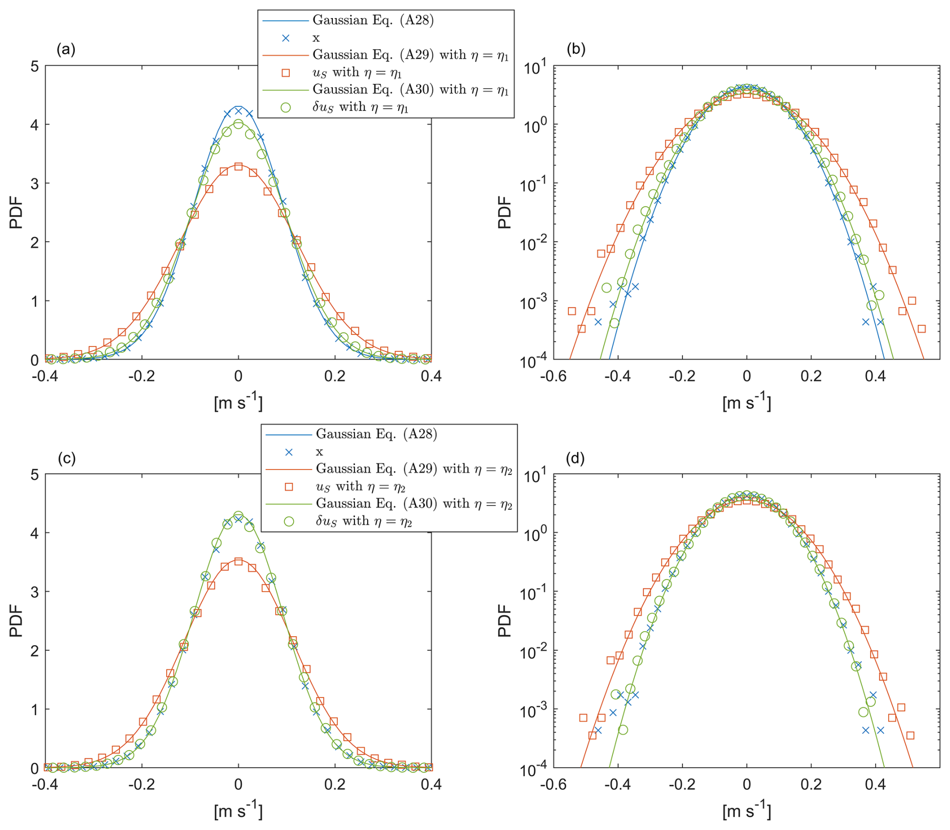
Figure A1 Gaussian PDFs of the stochastic variables x (in blue), u_S (in red) and δu_S (in green): the continuous lines are the analytical Gaussian PDFs in Eqs. (A29), (A30) and (A31), while the points are the histograms of the simulated variables described in Eqs. (A2) and (A17) in the case where Q= constant. The parameters used are shown in Table A1. The simulation results with η=η₁ are shown in (a) and (b), while in (c) and (d), the results with η=η₂ are shown. In (a) and (c), the plots are lin–lin, while in (b) and (d), the plots are lin–log.

Appendix B: Ornstein–Uhlenbeck processes and coloured noise

Let's consider the stochastic part for the u component (analogously for the v component) of the SUP model:

$$\begin{array}{}\text{(B1)}& {\displaystyle }\mathrm{d}{\mathit{\alpha }}_i=-\mathit{\mu }{\mathit{\alpha }}_i\mathrm{d}t+{\mathit{\beta }}_u\mathrm{d}{W}_i,\text{(B2)}& {\displaystyle }\mathrm{d}x=-{\mathit{\gamma }}_{x}x\mathrm{d}t+\sqrt{{\mathrm{\Sigma }}_{i=\mathrm{1}}^{\mathrm{2}\mathit{\nu }}{\mathit{\alpha }}_i^{\mathrm{2}}}\mathrm{d}{W}_x,\text{(B3)}& {\displaystyle }\mathrm{d}{u}_{\mathrm{S}}=-{\mathit{\gamma }}_u{u}_{\mathrm{S}}\mathrm{d}t+\mathit{\eta }x\mathrm{d}t.\end{array}$$

Because β and μ are constants, Eq. (B1) is a Langevin equation, and the variables α_i are Ornstein–Uhlenbeck processes; thus, their distribution in the stationary state is Gaussian:

$$\begin{array}{}\text{(B4)}& p_{\mathit{\alpha }}\left({\mathit{\alpha }}_i\right)=\sqrt{{\displaystyle \frac{\mathit{\mu }}{\mathit{\pi }{\mathit{\beta }}_u^{\mathrm{2}}}}}{e}^{-\mathit{\mu }{\mathit{\alpha }}_i^{\mathrm{2}}/{\mathit{\beta }}_u^{\mathrm{2}}}.\end{array}$$

Defining the new variable Q as the sum of 2ν squared identically distributed Gaussian variables $Q={\mathrm{\Sigma }}_{i=\mathrm{1}}^{\mathrm{2}\mathit{\nu }}{\mathit{\alpha }}_i^{\mathrm{2}}$ results in a variable distributed with a gamma distribution, with a shape parameter equal to ν in the stationary state:

$$\begin{array}{}\text{(B5)}& \begin{array}{rl}{p}_Q\left(Q\right)& ={\mathrm{\Gamma }}_{\mathit{\nu },\stackrel{\mathrm{̃}}{\mathit{\lambda }}}\left(Q\right)={\displaystyle \frac{{\stackrel{\mathrm{̃}}{\mathit{\lambda }}}^{\mathit{\nu }}{Q}^{\mathit{\nu }-\mathrm{1}}{e}^{-\stackrel{\mathrm{̃}}{\mathit{\lambda }}Q}}{\mathrm{\Gamma }\left(\mathit{\nu }\right)}}\\ & ={\left({\displaystyle \frac{\mathit{\mu }}{{\mathit{\beta }}_u^{\mathrm{2}}}}\right)}^{\mathit{\nu }}{\displaystyle \frac{Q^{\mathit{\nu }-\mathrm{1}}}{\mathrm{\Gamma }\left(\mathit{\nu }\right)}}{e}^{-\mathit{\mu }Q/{\mathit{\beta }}_u^{\mathrm{2}}},\end{array}\end{array}$$

where $\stackrel{\mathrm{̃}}{\mathit{\lambda }}=\frac{\mathit{\mu }}{{\mathit{\beta }}_u^{\mathrm{2}}}$ and the first moment is

$$\begin{array}{}\text{(B6)}& E\left[Q\right]=\underset{\mathrm{0}}{\overset{\mathrm{\infty }}{\int }}{\left({\displaystyle \frac{\mathit{\mu }}{{\mathit{\beta }}^{\mathrm{2}}}}\right)}^{\mathit{\nu }}{\displaystyle \frac{Q^{\mathit{\nu }}}{\mathrm{\Gamma }\left(\mathit{\nu }\right)}}{e}^{-\mathit{\mu }Q/{\mathit{\beta }}^{\mathrm{2}}}\mathrm{d}Q={\displaystyle \frac{\mathit{\nu }{\mathit{\beta }}^{\mathrm{2}}}{\mathit{\mu }}}.\end{array}$$

It is possible to write Eq. (B2) in the following way:

$$\begin{array}{}\text{(B7)}& \mathrm{d}x=-{\mathit{\gamma }}_{x}x\mathrm{d}t+\sqrt{Q}\mathrm{d}{W}_x.\end{array}$$

If Q were a constant, then the equation above would be a Langevin equation, and x would represent an Ornstein–Uhlenbeck process. However, by construction, Q slowly varies with respect to x (because $\mathit{\tau }=\frac{\mathrm{1}}{{\mathit{\gamma }}_x}\ll T=\frac{\mathrm{1}}{\mathit{\mu }}$). Thus, it is possible to assume that, locally in time, Q is constant, and therefore locally x has a Gaussian distribution, given a certain variance ${\mathit{\sigma }}_x^{\mathrm{2}}=\frac{Q}{\mathrm{2}{\mathit{\gamma }}_x}$ determined by the value of Q:

$$\begin{array}{}\text{(B8)}& \begin{array}{rl}p\left(x\right|{\mathit{\sigma }}_x^{\mathrm{2}})& =N\left(\mathrm{0},{\mathit{\sigma }}_x^{\mathrm{2}}\right)={\displaystyle \frac{\mathrm{1}}{\sqrt{\mathrm{2}\mathit{\pi }{\mathit{\sigma }}_x^{\mathrm{2}}}}}{e}^{-x^{\mathrm{2}}/\mathrm{2}{\mathit{\sigma }}_x^{\mathrm{2}}}\\ & =\sqrt{{\displaystyle \frac{{\mathit{\gamma }}_x}{\mathit{\pi }Q}}}{e}^{-{\mathit{\gamma }}_x{x}^{\mathrm{2}}/Q}.\end{array}\end{array}$$

In order to obtain the total x PDF, the ${\mathit{\sigma }}_x^{\mathrm{2}}$ PDF $f\left({\mathit{\sigma }}_x^{\mathrm{2}}\right)$ is needed. Thanks to its dependence on Q, it is possible to obtain it:

$$\begin{array}{}\text{(B9)}& \begin{array}{rl}f\left({\mathit{\sigma }}_x^{\mathrm{2}}\right)& ={\mathrm{\Gamma }}_{\mathit{\nu },\mathit{\lambda }}\left({\mathit{\sigma }}_x^{\mathrm{2}}\right)={\displaystyle \frac{{\mathit{\lambda }}^{\mathit{\nu }}{\mathit{\sigma }}_x^{\mathrm{2}(\mathit{\nu }-\mathrm{1})}{e}^{-\mathit{\lambda }{\mathit{\sigma }}_x^{\mathrm{2}}}}{\mathrm{\Gamma }\left(\mathit{\nu }\right)}}\\ & ={\left({\displaystyle \frac{\mathrm{2}\mathit{\mu }{\mathit{\gamma }}_x}{{\mathit{\beta }}_u^{\mathrm{2}}}}\right)}^{\mathit{\nu }}{\displaystyle \frac{{\mathit{\sigma }}_x^{\mathrm{2}(\mathit{\nu }-\mathrm{1})}}{\mathrm{\Gamma }\left(\mathit{\nu }\right)}}{e}^{-\frac{\mathrm{2}\mathit{\mu }{\mathit{\gamma }}_x}{{\mathit{\beta }}_u^{\mathrm{2}}}{\mathit{\sigma }}_x^{\mathrm{2}}},\end{array}\end{array}$$

where $\mathit{\lambda }=\frac{\mathrm{2}\mathit{\mu }{\mathit{\gamma }}_x}{{\mathit{\beta }}_u^{\mathrm{2}}}$. It follows that

$$\begin{array}{}\text{(B10)}& \begin{array}{rl}{p}_{\mathit{\nu }}\left(x\right)& =\underset{\mathrm{0}}{\overset{\mathrm{\infty }}{\int }}f\left({\mathit{\sigma }}_x^{\mathrm{2}}\right)p\left(x\right|{\mathit{\sigma }}_x^{\mathrm{2}})d{\mathit{\sigma }}_x^{\mathrm{2}}\\ & ={\displaystyle \frac{{\mathit{\lambda }}^{\mathit{\nu }}}{\mathrm{\Gamma }\left(\mathit{\nu }\right)\sqrt{\mathrm{2}\mathit{\pi }}}}\underset{\mathrm{0}}{\overset{\mathrm{\infty }}{\int }}{\mathit{\sigma }}_x^{\mathrm{2}(\mathit{\nu }-\mathrm{1})}{e}^{-\mathit{\lambda }{\mathit{\sigma }}_x^{\mathrm{2}}}\\ & {\displaystyle \frac{\mathrm{1}}{\sqrt{{\mathit{\sigma }}_x^{\mathrm{2}}}}}{e}^{-x^{\mathrm{2}}/\mathrm{2}{\mathit{\sigma }}_x^{\mathrm{2}}}\mathrm{d}\left({\mathit{\sigma }}_x^{\mathrm{2}}\right)\\ & ={\displaystyle \frac{{\mathit{\lambda }}^{\mathit{\nu }}}{\mathrm{\Gamma }\left(\mathit{\nu }\right)\sqrt{\mathrm{2}\mathit{\pi }}}}\underset{\mathrm{0}}{\overset{\mathrm{\infty }}{\int }}{z}^{\mathit{\nu }-\mathrm{3}/\mathrm{2}}{e}^{-\mathit{\lambda }z-x^{\mathrm{2}}/\mathrm{2}z}\mathrm{d}z,\end{array}\end{array}$$

which, for ν=2, gives the following result (Gradshteyn and Ryzhik, 2014, p. 369, Eq. 3.471.16), called the Exp-Lin PDF in this paper:

$$\begin{array}{}\text{(B11)}& \begin{array}{rl}{p}_{\mathit{\nu }=\mathrm{2}}\left(x\right)& =-{\displaystyle \frac{{\mathit{\lambda }}^{\mathrm{2}}}{\sqrt{\mathrm{2}}}}{\displaystyle \frac{\partial }{\partial \mathit{\lambda }}}\left({\mathit{\lambda }}^{-\mathrm{1}/\mathrm{2}}{e}^{-\sqrt{\mathrm{2}\mathit{\lambda }}\left|x\right|}\right)\\ & ={\displaystyle \frac{\sqrt{\mathrm{2}\mathit{\lambda }}{e}^{-\sqrt{\mathrm{2}\mathit{\lambda }}\left|x\right|}\left(\sqrt{\mathrm{2}\mathit{\lambda }}\right|x|+\mathrm{1})}{\mathrm{4}}}\\ & ={\displaystyle \frac{\sqrt{\mathit{\mu }{\mathit{\gamma }}_x}}{\mathrm{2}{\mathit{\beta }}_u}}{e}^{-\mathrm{2}\sqrt{\mathit{\mu }{\mathit{\gamma }}_x}\left|x\right|/{\mathit{\beta }}_u}\left({\displaystyle \frac{\mathrm{2}\sqrt{\mathit{\mu }{\mathit{\gamma }}_x}}{{\mathit{\beta }}_u}}\left|x\right|+\mathrm{1}\right).\end{array}\end{array}$$

Meanwhile, for $\mathit{\nu }=\mathrm{1}/\mathrm{2}$ (Gradshteyn and Ryzhik, 2014, p. 370, Eq. 3.478.4),

$$\begin{array}{}\text{(B12)}& \begin{array}{rl}{p}_{\mathit{\nu }=\frac{\mathrm{1}}{\mathrm{2}}}\left(x\right)& ={\displaystyle \frac{\sqrt{\mathrm{2}\mathit{\lambda }}}{\mathit{\pi }}}{K}_{\mathrm{0}}\left(\sqrt{\mathrm{2}\mathit{\lambda }}\left|x\right|\right)\\ & ={\displaystyle \frac{\mathrm{2}\sqrt{\mathit{\mu }{\mathit{\gamma }}_x}}{\mathit{\pi }{\mathit{\beta }}_u}}{K}_{\mathrm{0}}\left({\displaystyle \frac{\mathrm{2}\sqrt{\mathit{\mu }{\mathit{\gamma }}_x}}{{\mathit{\beta }}_u}}\left|x\right|\right),\end{array}\end{array}$$

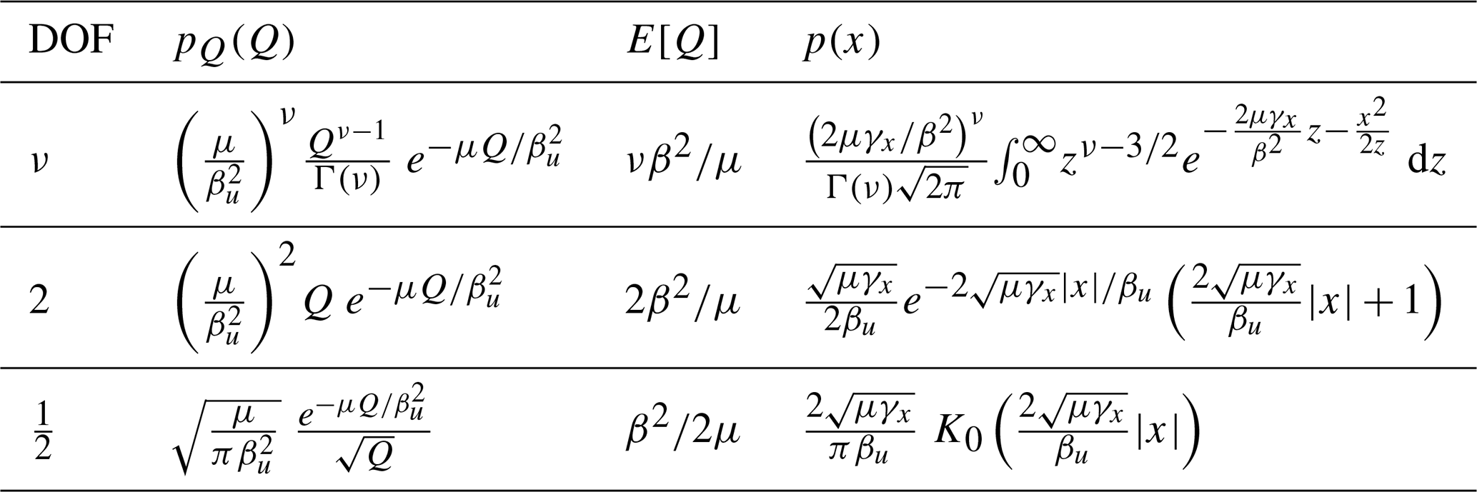
where K₀(z) is the modified Bessel function of the second kind of zero order. A summary of the results of this Appendix for the cases ν, 2 and $\mathrm{1}/\mathrm{2}$ degrees of freedom (DOFs) is given in Table B1. Finally, Eq. (B3) does not present any analytic solution.

Table B1 Analytical PDFs and means of the variable Q and analytical PDFs of the variable x for ν, 2 and 1/2 degrees of freedom.

Appendix C: The Ekman system of the deterministic model – the linear relation of the coefficients with wind speed

Defining the energy $E=\stackrel{\mathrm{̃}}{h}\frac{|{\mathit{u}}_o{|}^{\mathrm{2}}}{\mathrm{2}}$ for the DET model in Eq. (1) and supposing, as a first approximation, that the tidal signal is negligible u_o≃u_E (daily timescale), assuming a slowly varying sea surface layer depth ${\partial }_t\stackrel{\mathrm{̃}}{h}=\mathrm{0}$ and neglecting the eddy depletion term $\mathit{F}={\mathit{\rho }}_{\mathrm{a}}{c}_a\left|{\mathit{u}}_{\mathrm{a}}\right|{\mathit{u}}_{\mathrm{a}}$, the energy variation in time can be expressed as follows:

$$\begin{array}{}\text{(C1)}& \begin{array}{rl}{\partial }_{t}E& =\stackrel{\mathrm{̃}}{h}{\partial }_t{\displaystyle \frac{|{\mathit{u}}_{\mathrm{E}}{|}^{\mathrm{2}}}{\mathrm{2}}}=\stackrel{\mathrm{̃}}{h}\left(u_{\mathrm{E}}{\partial }_t{u}_{\mathrm{E}}+v_{\mathrm{E}}{\partial }_t{v}_{\mathrm{E}}\right)\\ & =-C_B|{\mathit{u}}_{\mathrm{E}}{|}^{\mathrm{3}}+u_{\mathrm{E}}{F}_u+v_{\mathrm{E}}{F}_v,\end{array}\end{array}$$

from which

$$\begin{array}{}\text{(C2)}& {\displaystyle \frac{C_B}{\stackrel{\mathrm{̃}}{h}}}={\displaystyle \frac{u_{\mathrm{E}}{F}_u+v_{\mathrm{E}}{F}_v}{\stackrel{\mathrm{̃}}{h}|{\mathit{u}}_{\mathrm{E}}{|}^{\mathrm{3}}}}-{\displaystyle \frac{{\partial }_t|{\mathit{u}}_{\mathrm{E}}{|}^{\mathrm{2}}}{\mathrm{2}|{\mathit{u}}_{\mathrm{E}}{|}^{\mathrm{3}}}}.\end{array}$$

Discretizing Eqs. (C1) and (C2) around the time step t_i (where $\mathrm{\Delta }t=t_{i+\mathrm{1}}-t_i$) and using the centred scheme for the temporal derivative ${\partial }_t|{\mathit{u}}_{\mathrm{E}}{|}^{\mathrm{2}}=\frac{\left|{\mathit{u}}_{\mathrm{E}}\right(t_{i+\mathrm{1}}){|}^{\mathrm{2}}-|{\mathit{u}}_{\mathrm{E}}\left(t_{i-\mathrm{1}}\right){|}^{\mathrm{2}}}{\mathrm{2}\mathrm{\Delta }t}$) result in the following:

$$\begin{array}{}\text{(C3)}& \begin{array}{rl}\stackrel{\mathrm{̃}}{h}& {\displaystyle \frac{\left|{\mathit{u}}_{\mathrm{E}}\right(t_{i+\mathrm{1}}){|}^{\mathrm{2}}-|{\mathit{u}}_{\mathrm{E}}\left(t_{i-\mathrm{1}}\right){|}^{\mathrm{2}}}{\mathrm{4}}}=-C_B\left(t_i\right)\left|{\mathit{u}}_{\mathrm{E}}\right(t_i){|}^{\mathrm{3}}\mathrm{\Delta }t\\ & +\left[u_{\mathrm{E}}\left(t_i\right)F_u\left(t_i\right)+v_{\mathrm{E}}\left(t_i\right)F_v\left(t_i\right)\right]\mathrm{\Delta }t\end{array}\end{array}$$

and

$$\begin{array}{}\text{(C4)}& \begin{array}{rl}{\displaystyle \frac{C_B\left(t_i\right)}{\stackrel{\mathrm{̃}}{h}}}& ={\displaystyle \frac{u_{\mathrm{E}}\left(t_i\right)F_u\left(t_i\right)+v_{\mathrm{E}}\left(t_i\right)F_v\left(t_i\right)}{\stackrel{\mathrm{̃}}{h}\left|{\mathit{u}}_{\mathrm{E}}\right(t_i){|}^{\mathrm{3}}}}\\ & -{\displaystyle \frac{\left|{\mathit{u}}_{\mathrm{E}}\right(t_{i+\mathrm{1}}){|}^{\mathrm{2}}-|{\mathit{u}}_{\mathrm{E}}\left(t_{i-\mathrm{1}}\right){|}^{\mathrm{2}}}{\mathrm{4}\left|{\mathit{u}}_{\mathrm{E}}\right(t_i){|}^{\mathrm{3}}\mathrm{\Delta }t}}\\ & ={\displaystyle \frac{\mathit{\alpha }\left(t_i\right)}{\stackrel{\mathrm{̃}}{h}}}-\mathit{\zeta }\left(t_i\right),\end{array}\end{array}$$

where $\mathit{\alpha }\left(t_i\right)=\frac{u_{\mathrm{E}}\left(t_i\right)F_u\left(t_i\right)+v_{\mathrm{E}}\left(t_i\right)F_v\left(t_i\right)}{\left|{\mathit{u}}_{\mathrm{E}}\right(t_i){|}^{\mathrm{3}}}$, $\mathit{\zeta }\left(t_i\right)=\frac{\left|{\mathit{u}}_{\mathrm{E}}\right(t_i+\mathrm{\Delta }t){|}^{\mathrm{2}}-|{\mathit{u}}_{\mathrm{E}}(t_i-\mathrm{\Delta }t){|}^{\mathrm{2}}}{\mathrm{4}\left|{\mathit{u}}_{\mathrm{E}}\right(t_i){|}^{\mathrm{3}}\mathrm{\Delta }t}$ and $\stackrel{\mathrm{̃}}{h}$ has a low dependence on time. Approximating the daily averaged observed sea surface current as the daily deterministic Ekman sea surface current, it is possible to calculate the coefficients α(t_i) and ζ(t_i) directly from the observations and the daily averaged wind forcing.

Equation (1) results in

$$\begin{array}{}\text{(C5)}& \begin{array}{rl}\left(\begin{array}{c}{\partial }_t{u}_{\mathrm{E}}\\ {\partial }_t{v}_{\mathrm{E}}\end{array}\right)& =\left(\begin{array}{cc}-\left(\frac{\mathit{\alpha }}{\stackrel{\mathrm{̃}}{h}}-\mathit{\zeta }\right)\left|{\mathit{u}}_{\mathrm{E}}\right|& f\\ -f& -\left(\frac{\mathit{\alpha }}{\stackrel{\mathrm{̃}}{h}}-\mathit{\zeta }\right)\left|{\mathit{u}}_{\mathrm{E}}\right|\end{array}\right)\\ & \left(\begin{array}{c}{u}_{\mathrm{E}}\\ v_{\mathrm{E}}\end{array}\right)+\left(\begin{array}{c}\frac{F_u}{\stackrel{\mathrm{̃}}{h}}\\ \frac{F_v}{\stackrel{\mathrm{̃}}{h}}\end{array}\right),\end{array}\end{array}$$

$$\begin{array}{}\text{(C6)}& \left\{\begin{array}{l}{\partial }_t{u}_{\mathrm{E}}-\mathit{\zeta }\left|{\mathit{u}}_{\mathrm{E}}\right|u_{\mathrm{E}}-f{v}_{\mathrm{E}}=\frac{F_u-\mathit{\alpha }\left|{\mathit{u}}_{\mathrm{E}}\right|u_{\mathrm{E}}}{\stackrel{\mathrm{̃}}{h}}\\ {\partial }_t{v}_{\mathrm{E}}-\mathit{\zeta }\left|{\mathit{u}}_{\mathrm{E}}\right|v_{\mathrm{E}}+f{u}_{\mathrm{E}}=\frac{F_v-\mathit{\alpha }\left|{\mathit{u}}_{\mathrm{E}}\right|v_{\mathrm{E}}}{\stackrel{\mathrm{̃}}{h}}\end{array}\right.,\end{array}$$

from which it is possible to obtain the slowly varying $\stackrel{\mathrm{̃}}{h}$:

$$\begin{array}{}\text{(C7)}& \left\{\begin{array}{l}\stackrel{\mathrm{̃}}{h}=\frac{F_u-\mathit{\alpha }\left|{\mathit{u}}_{\mathrm{E}}\right|u_{\mathrm{E}}}{{\partial }_t{u}_{\mathrm{E}}-\mathit{\zeta }\left|{\mathit{u}}_{\mathrm{E}}\right|u_{\mathrm{E}}-f{v}_{\mathrm{E}}}\\ \stackrel{\mathrm{̃}}{h}=\frac{F_v-\mathit{\alpha }\left|{\mathit{u}}_{\mathrm{E}}\right|v_{\mathrm{E}}}{{\partial }_t{v}_{\mathrm{E}}-\mathit{\zeta }\left|{\mathit{u}}_{\mathrm{E}}\right|v_{\mathrm{E}}+f{u}_{\mathrm{E}}}\end{array}\right..\end{array}$$

The discretization gives

$$\begin{array}{}\text{(C8)}& \left\{\begin{array}{l}\stackrel{\mathrm{̃}}{h}\left(t_i\right)=\frac{F_u\left(t_i\right)-\mathit{\alpha }\left(t_i\right)\left|{\mathit{u}}_{\mathrm{E}}\right(t_i\left)\right|u_{\mathrm{E}}\left(t_i\right)}{\left[u_{\mathrm{E}}(t_i+\mathrm{\Delta }t)-u_{\mathrm{E}}(t_i-\mathrm{\Delta }t)\right]/\mathrm{2}\mathrm{\Delta }t-\mathit{\zeta }\left(t_i\right)\left|{\mathit{u}}_{\mathrm{E}}\right(t_i\left)\right|u_{\mathrm{E}}\left(t_i\right)-f{v}_D\left(t_i\right)}\\ \stackrel{\mathrm{̃}}{h}\left(t_i\right)=\frac{F_v\left(t_i\right)-\mathit{\alpha }\left(t_i\right)\left|{\mathit{u}}_{\mathrm{E}}\right(t_i\left)\right|v_{\mathrm{E}}\left(t_i\right)}{\left[v_{\mathrm{E}}(t_i+\mathrm{\Delta }t)-v_{\mathrm{E}}(t_i-\mathrm{\Delta }t)\right]/\mathrm{2}\mathrm{\Delta }t-\mathit{\zeta }\left(t_i\right)\left|{\mathit{u}}_{\mathrm{E}}\right(t_i\left)\right|v_{\mathrm{E}}\left(t_i\right)+f{u}_{\mathrm{E}}\left(t_i\right)}\end{array}\right..\end{array}$$

The two expressions in Eq. (C8) should give a unique value for $\stackrel{\mathrm{̃}}{h}$ as a function of time directly from the daily averaged observed currents and the daily averaged wind forcing. In practice, they almost agree, and we calculated $\stackrel{\mathrm{̃}}{h}\left(t_i\right)$ as the average of these two expressions. From $\stackrel{\mathrm{̃}}{h}\left(t_i\right)$, it is also possible to obtain C_B(t_i):

$$\begin{array}{}\text{(C9)}& C_B\left(t_i\right)=\mathit{\alpha }\left(t_i\right)-\mathit{\zeta }\left(t_i\right)\cdot \stackrel{\mathrm{̃}}{h}\left(t_i\right).\end{array}$$

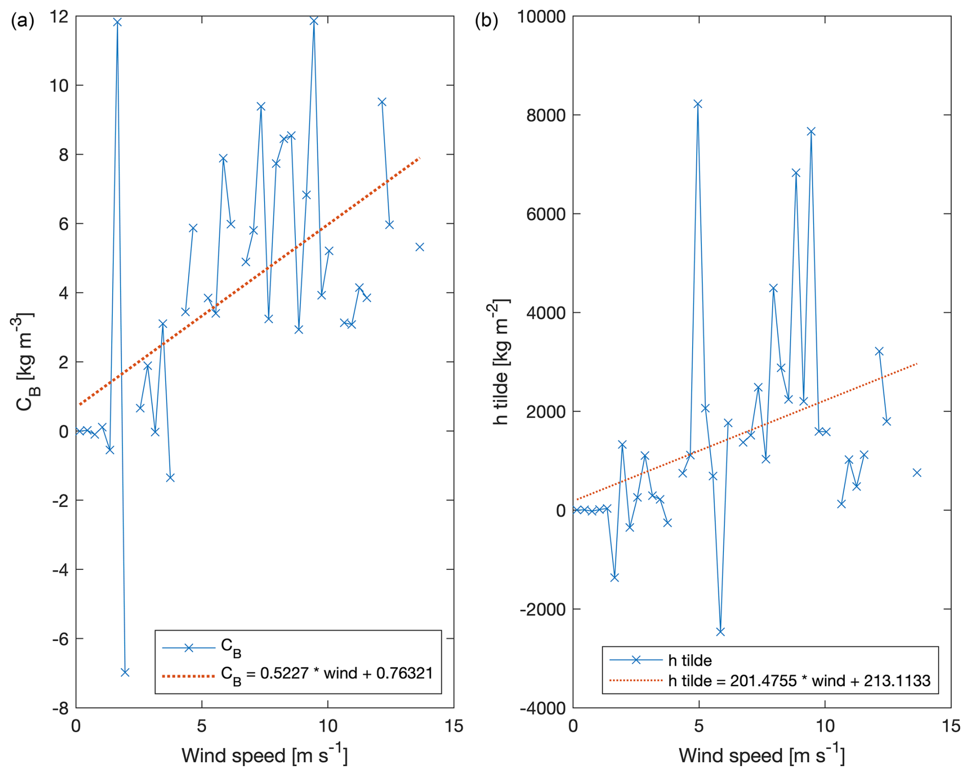
Having the $\stackrel{\mathrm{̃}}{h}$, C_B and wind speed time series, it is possible to calculate the mean values of $\stackrel{\mathrm{̃}}{h}$ and C_B as a function of the wind speed, obtaining a linear fit after deleting the values exceeding 1 standard deviation (Fig. C1).

Figure C1 Dependence on wind speed of the model coefficients C_B and $\stackrel{\mathrm{̃}}{h}$, calculated according to Eq. (C9) and to the mean of Eq. (C8), respectively, and their linear regressions.

Appendix D: On the Ekman angle standard deviation

In this study, the Ekman angle is defined as the angle between the daily wind and the daily sea surface current; it is positive if the sea surface current is on the right with respect to the wind direction. For simplicity, it is assumed that the wind does not contribute with any error and is perfectly known. It follows that the standard deviation of the Ekman angle coincides with the standard deviation of the daily sea surface current angle. Under this assumption, the given Ekman angle standard deviation is an underestimation of its real error. Thus, in order to obtain this estimation of the Ekman angle standard deviation, starting from the modelled (HFR measured) sea surface current components with a 5 min (30 min) time resolution and their stochastic variability (measure accuracy), two points must be followed: (i) the daily average transformation and (ii) the polar coordinates transformation.

Let's take into consideration the sea surface currents time series of a single day $x=\mathit{\{}{u}_{\mathrm{1}},\mathrm{\dots },u_n,v_{\mathrm{1}},\mathrm{\dots }{v}_n\mathit{\}}$, where n=288 for the 5 min time resolution modelled sea surface currents and n=48 for the 30 min HFR observed sea surface currents, with their 2n×2n symmetric covariance matrix:

$$\begin{array}{}\text{(D1)}& \begin{array}{rl}{\mathrm{\Sigma }}^x& =\left(\begin{array}{cccccc}{\mathit{\sigma }}_{u_{\mathrm{1}}}^{\mathrm{2}}& \mathrm{\cdots }& {\mathit{\sigma }}_{u_{\mathrm{1}}{u}_n}& {\mathit{\sigma }}_{u_{\mathrm{1}}{v}_{\mathrm{1}}}& \mathrm{\cdots }& {\mathit{\sigma }}_{u_{\mathrm{1}}{v}_n}\\ \mathrm{⋮}& \mathrm{\ddots }& \mathrm{⋮}& \mathrm{⋮}& & \mathrm{⋮}\\ {\mathit{\sigma }}_{u_n{u}_{\mathrm{1}}}& \mathrm{\cdots }& {\mathit{\sigma }}_{u_n}^{\mathrm{2}}& {\mathit{\sigma }}_{u_n{v}_{\mathrm{1}}}& \mathrm{\cdots }& {\mathit{\sigma }}_{u_n{v}_n}\\ {\mathit{\sigma }}_{v_{\mathrm{1}}{u}_{\mathrm{1}}}& \mathrm{\cdots }& {\mathit{\sigma }}_{v_{\mathrm{1}}{u}_n}& {\mathit{\sigma }}_{v_{\mathrm{1}}}^{\mathrm{2}}& \mathrm{\cdots }& {\mathit{\sigma }}_{v_{\mathrm{1}}{v}_n}\\ \mathrm{⋮}& & \mathrm{⋮}& \mathrm{⋮}& \mathrm{\ddots }& \mathrm{⋮}\\ {\mathit{\sigma }}_{v_n{u}_{\mathrm{1}}}& \mathrm{\cdots }& {\mathit{\sigma }}_{v_n{u}_n}& {\mathit{\sigma }}_{v_n{v}_{\mathrm{1}}}& \mathrm{\cdots }& {\mathit{\sigma }}_{v_n}^{\mathrm{2}}\end{array}\right)\\ & =\left(\begin{array}{cc}{\mathrm{\Sigma }}_{uu}^x& {\mathrm{\Sigma }}_{uv}^x\\ {\mathrm{\Sigma }}_{uv}^x& {\mathrm{\Sigma }}_{vv}^x\end{array}\right).\end{array}\end{array}$$

Here, the sea surface currents are the ensemble averaged values for each time, and the covariance matrix values are the relative ensemble variances and covariances, while for the observations, the sea surface currents are simply the independent HFR measured sea surface currents (each measurement is independent from the others) with their HFR accuracy and zero covariances (thus, Σ^x reduces to a diagonal matrix).

Calling $f=\left(\begin{array}{c}\overline{u}\\ \overline{v}\end{array}\right)$ the daily average sea surface currents for a single day, its linear transformation (here, the transformation matrix is called A) can be written as

$$\begin{array}{}\text{(D2)}& {\displaystyle }f=A\cdot x,\text{(D3)}& {\displaystyle }\left(\begin{array}{c}\overline{u}\\ \overline{v}\end{array}\right)={\displaystyle \frac{\mathrm{1}}{n}}\left(\begin{array}{cc}\stackrel{n}{\overbrace{\mathrm{1}\mathrm{\cdots }\mathrm{1}}}& \stackrel{n}{\overbrace{\mathrm{0}\mathrm{\cdots }\mathrm{0}}}\\ \underset{n}{\underbrace{\mathrm{0}\mathrm{\cdots }\mathrm{0}}}& \underset{n}{\underbrace{\mathrm{1}\mathrm{\cdots }\mathrm{1}}}\end{array}\right)\left(\begin{array}{c}{u}_{\mathrm{1}}\\ \mathrm{⋮}\\ u_n\\ v_{\mathrm{1}}\\ \mathrm{⋮}\\ v_n\end{array}\right).\end{array}$$

Thus, the covariance matrix of the transformed variable ${\mathrm{\Sigma }}^f=\left(\begin{array}{cc}{\mathit{\sigma }}_{\overline{u}}^{\mathrm{2}}& {\mathit{\sigma }}_{\overline{u}\overline{v}}\\ {\mathit{\sigma }}_{\overline{u}\overline{v}}& {\mathit{\sigma }}_{\overline{v}}^{\mathrm{2}}\end{array}\right)$ can be obtained in the following way:

$$\begin{array}{}\text{(D4)}& \begin{array}{rl}{\mathrm{\Sigma }}^f& =A\cdot {\mathrm{\Sigma }}^x\cdot A^T\\ & ={\displaystyle \frac{\mathrm{1}}{n^{\mathrm{2}}}}\left(\begin{array}{cccccc}\mathrm{1}& \mathrm{\cdots }& \mathrm{1}& \mathrm{0}& \mathrm{\cdots }& \mathrm{0}\\ \mathrm{0}& \mathrm{\cdots }& \mathrm{0}& \mathrm{1}& \mathrm{\cdots }& \mathrm{1}\end{array}\right)\\ & \left(\begin{array}{cccccc}{\mathit{\sigma }}_{u_{\mathrm{1}}}^{\mathrm{2}}& \mathrm{\cdots }& {\mathit{\sigma }}_{u_{\mathrm{1}}{u}_n}& {\mathit{\sigma }}_{u_{\mathrm{1}}{v}_{\mathrm{1}}}& \mathrm{\cdots }& {\mathit{\sigma }}_{u_{\mathrm{1}}{v}_n}\\ \mathrm{⋮}& \mathrm{\ddots }& \mathrm{⋮}& \mathrm{⋮}& & \mathrm{⋮}\\ {\mathit{\sigma }}_{u_n{u}_{\mathrm{1}}}& \mathrm{\cdots }& {\mathit{\sigma }}_{u_n}^{\mathrm{2}}& {\mathit{\sigma }}_{u_n{v}_{\mathrm{1}}}& \mathrm{\cdots }& {\mathit{\sigma }}_{u_n{v}_n}\\ {\mathit{\sigma }}_{v_{\mathrm{1}}{u}_{\mathrm{1}}}& \mathrm{\cdots }& {\mathit{\sigma }}_{v_{\mathrm{1}}{u}_n}& {\mathit{\sigma }}_{v_{\mathrm{1}}}^{\mathrm{2}}& \mathrm{\cdots }& {\mathit{\sigma }}_{v_{\mathrm{1}}{v}_n}\\ \mathrm{⋮}& & \mathrm{⋮}& \mathrm{⋮}& \mathrm{\ddots }& \mathrm{⋮}\\ {\mathit{\sigma }}_{v_n{u}_{\mathrm{1}}}& \mathrm{\cdots }& {\mathit{\sigma }}_{v_n{u}_n}& {\mathit{\sigma }}_{v_n{v}_{\mathrm{1}}}& \mathrm{\cdots }& {\mathit{\sigma }}_{v_n}^{\mathrm{2}}\end{array}\right)\left(\begin{array}{cc}\mathrm{1}& \mathrm{0}\\ \mathrm{⋮}& \mathrm{⋮}\\ \mathrm{1}& \mathrm{0}\\ \mathrm{0}& \mathrm{1}\\ \mathrm{⋮}& \mathrm{⋮}\\ \mathrm{0}& \mathrm{1}\end{array}\right)\\ & ={\displaystyle \frac{\mathrm{1}}{n^{\mathrm{2}}}}\left(\begin{array}{cc}\text{sum}\left({\mathrm{\Sigma }}_{uu}^x\right)& \text{sum}\left({\mathrm{\Sigma }}_{uv}^x\right)\\ \text{sum}\left({\mathrm{\Sigma }}_{uv}^x\right)& \text{sum}\left({\mathrm{\Sigma }}_{vv}^x\right)\end{array}\right).\end{array}\end{array}$$

Once the daily sea surface current components $\left(\begin{array}{c}\overline{u}\\ \overline{v}\end{array}\right)$ and their covariance matrix $\left(\begin{array}{cc}{\mathit{\sigma }}_{\overline{u}}^{\mathrm{2}}& {\mathit{\sigma }}_{\overline{u}\overline{v}}\\ {\mathit{\sigma }}_{\overline{u}\overline{v}}& {\mathit{\sigma }}_{\overline{v}}^{\mathrm{2}}\end{array}\right)$ are obtained, it is possible to change from Cartesian to polar coordinates:

$$\begin{array}{}\text{(D5)}& \left\{\begin{array}{l}r=\sqrt{{\overline{u}}^{\mathrm{2}}+{\overline{v}}^{\mathrm{2}}}\\ \mathit{\theta }=\arctan \left(\frac{\overline{v}}{\overline{u}}\right)\end{array}\right..\end{array}$$

The transformation now is not linear, and one must resort to the Jacobian matrix:

$$\begin{array}{}\text{(D6)}& J=\left(\begin{array}{cc}\frac{\partial r}{\partial \overline{u}}& \frac{\partial r}{\partial \overline{v}}\\ \frac{\partial \mathit{\theta }}{\partial \overline{u}}& \frac{\partial \mathit{\theta }}{\partial \overline{v}}\end{array}\right)=\left(\begin{array}{cc}\frac{\overline{u}}{\sqrt{{\overline{u}}^{\mathrm{2}}+{\overline{v}}^{\mathrm{2}}}}& \frac{\overline{v}}{\sqrt{{\overline{u}}^{\mathrm{2}}+{\overline{v}}^{\mathrm{2}}}}\\ -\frac{\overline{v}}{{\overline{u}}^{\mathrm{2}}+{\overline{v}}^{\mathrm{2}}}& \frac{\overline{u}}{{\overline{u}}^{\mathrm{2}}+{\overline{v}}^{\mathrm{2}}}\end{array}\right)\end{array}$$

to obtain the new covariance matrix (θ and σ_θ are in radians):

$$\begin{array}{}\text{(D7)}& \begin{array}{rl}& \left(\begin{array}{cc}{\mathit{\sigma }}_r^{\mathrm{2}}& {\mathit{\sigma }}_{r\mathit{\theta }}\\ {\mathit{\sigma }}_{r\mathit{\theta }}& {\mathit{\sigma }}_{\mathit{\theta }}^{\mathrm{2}}\end{array}\right)=J\left(\begin{array}{cc}{\mathit{\sigma }}_{\overline{u}}^{\mathrm{2}}& {\mathit{\sigma }}_{\overline{u}\overline{v}}\\ {\mathit{\sigma }}_{\overline{u}\overline{v}}& {\mathit{\sigma }}_{\overline{v}}^{\mathrm{2}}\end{array}\right)J^T\\ & =\left(\begin{array}{cc}\frac{\overline{u}}{\sqrt{{\overline{u}}^{\mathrm{2}}+{\overline{v}}^{\mathrm{2}}}}& \frac{\overline{v}}{\sqrt{{\overline{u}}^{\mathrm{2}}+{\overline{v}}^{\mathrm{2}}}}\\ -\frac{\overline{v}}{{\overline{u}}^{\mathrm{2}}+{\overline{v}}^{\mathrm{2}}}& \frac{\overline{u}}{{\overline{u}}^{\mathrm{2}}+{\overline{v}}^{\mathrm{2}}}\end{array}\right)\left(\begin{array}{cc}{\mathit{\sigma }}_{\overline{u}}^{\mathrm{2}}& {\mathit{\sigma }}_{\overline{u}\overline{v}}\\ {\mathit{\sigma }}_{\overline{u}\overline{v}}& {\mathit{\sigma }}_{\overline{v}}^{\mathrm{2}}\end{array}\right)\left(\begin{array}{cc}\frac{\overline{u}}{\sqrt{{\overline{u}}^{\mathrm{2}}+{\overline{v}}^{\mathrm{2}}}}& -\frac{\overline{v}}{{\overline{u}}^{\mathrm{2}}+{\overline{v}}^{\mathrm{2}}}\\ \frac{\overline{v}}{\sqrt{{\overline{u}}^{\mathrm{2}}+{\overline{v}}^{\mathrm{2}}}}& \frac{\overline{u}}{{\overline{u}}^{\mathrm{2}}+{\overline{v}}^{\mathrm{2}}}\end{array}\right)\\ & =\left(\begin{array}{cc}\frac{{\overline{u}}^{\mathrm{2}}{\mathit{\sigma }}_{\overline{u}}^{\mathrm{2}}+\mathrm{2}\overline{u}\overline{v}{\mathit{\sigma }}_{\overline{u}\overline{v}}+{\overline{v}}^{\mathrm{2}}{\mathit{\sigma }}_{\overline{v}}^{\mathrm{2}}}{{\overline{u}}^{\mathrm{2}}+{\overline{v}}^{\mathrm{2}}}& \frac{-\overline{u}\overline{v}{\mathit{\sigma }}_{\overline{u}}^{\mathrm{2}}+{\left({\overline{u}}^{\mathrm{2}}-{\overline{v}}^{\mathrm{2}}\right)}^{\mathrm{2}}{\mathit{\sigma }}_{\overline{u}\overline{v}}+\overline{u}\overline{v}{\mathit{\sigma }}_{\overline{v}}^{\mathrm{2}}}{{\left({\overline{u}}^{\mathrm{2}}+{\overline{v}}^{\mathrm{2}}\right)}^{\mathrm{3}/\mathrm{2}}}\\ \frac{-\overline{u}\overline{v}{\mathit{\sigma }}_{\overline{u}}^{\mathrm{2}}+{\left({\overline{u}}^{\mathrm{2}}-{\overline{v}}^{\mathrm{2}}\right)}^{\mathrm{2}}{\mathit{\sigma }}_{\overline{u}\overline{v}}+\overline{u}\overline{v}{\mathit{\sigma }}_{\overline{v}}^{\mathrm{2}}}{{\left({\overline{u}}^{\mathrm{2}}+{\overline{v}}^{\mathrm{2}}\right)}^{\mathrm{3}/\mathrm{2}}}& \frac{{\overline{v}}^{\mathrm{2}}{\mathit{\sigma }}_{\overline{u}}^{\mathrm{2}}-\mathrm{2}\overline{u}\overline{v}{\mathit{\sigma }}_{\overline{u}\overline{v}}+{\overline{u}}^{\mathrm{2}}{\mathit{\sigma }}_{\overline{v}}^{\mathrm{2}}}{{\left({\overline{u}}^{\mathrm{2}}+{\overline{v}}^{\mathrm{2}}\right)}^{\mathrm{2}}}\end{array}\right).\end{array}\end{array}$$

The Ekman angle standard deviation is then taken as follows:

$$\begin{array}{}\text{(D8)}& {\mathit{\sigma }}_{{\mathit{\theta }}_{\mathrm{E}}}=\text{min}\left({\mathit{\sigma }}_{\mathit{\theta }},\mathit{\pi }\right).\end{array}$$