Optimized dynamic mode decomposition for reconstruction and forecasting of atmospheric chemistry data

We introduce the optimized dynamic mode decomposition (DMD) algorithm for constructing an adaptive and computationally efficient reduced-order model and forecasting tool for global atmospheric chemistry dynamics. By exploiting a low-dimensional set of global spatio-temporal modes, interpretable characterizations of the underlying spatial and temporal scales can be computed. Forecasting is also achieved with a linear model that uses a linear superposition of the dominant spatio-temporal features. The DMD method is demonstrated on 3 months of global chemistry dynamics data, showing its significant performance in terms of computational speed and interpretability. We show that the presented decomposition method successfully extracts and forecasts chemical patterns for leading chemical indicators, including nitric oxide, ozone, nitrogen dioxide, hydroxyl radical, isoprene, and carbon monoxide. Moreover, the DMD algorithm allows for rapid reconstruction of the underlying linear model, which can then easily accommodate non-stationary data and changes in the dynamics.

1 Introduction

The monitoring and forecasting of global atmospheric chemistry is critical for understanding the effects of air quality, chemistry–climate interactions, and global biogeochemical cycling (Jacob, 1999). The dynamics of atmospheric chemistry is characterized by complex interactions among hundreds of chemical species, which can produce kinetics across temporal scales spanning many orders of magnitude – from microseconds to years. Accurate monitoring and prediction require full knowledge of the chemical state of the atmosphere at all locations and times, resulting in a 4-dimensional data set for longitude, latitude, elevation, and time for each chemical species that can become massive as the resolution of each dimension is increased. Dimensionality reduction is a critically enabling aspect of machine learning and data science (Brunton and Kutz, 2019) that can be leveraged to approximate the monitoring and forecasting capabilities of global chemistry with more readily tractable computational algorithms (Velegar et al., 2019). Dynamic mode decomposition (DMD) is a data-driven regression architecture for adaptively learning linear dynamics models over snapshots of temporal data, specifically in a low-dimensional subspace. DMD has been broadly used in the scientific community due to its ease of use, interpretability, and adaptive nature (Kutz et al., 2016a). When applied to the spatio-temporal dynamics of atmospheric chemistry, we demonstrate that the method provides an effective and computationally efficient reduced-order modeling strategy that can be used for the characterization, monitoring, and forecasting of global chemical concentrations with either computational or sensor data. Moreover, we show that the optimized DMD algorithm (Askham and Kutz, 2018) and bagging optimized DMD (BOP-DMD) (Sashidhar and Kutz, 2022) versions of the DMD algorithm are critical for characterizing the complexities of the chemical interaction dynamics and their uncertainties.

Characterization of the multiscale phenomenon, such as that embodied by global atmospheric chemistry, remains challenging due to the need to resolve spatial and temporal scales that are separated by many orders of magnitude. Computational methods, which are typically based upon the underlying partial differential equations that model the governing dynamics, easily become intractable due to the need to resolve the finest space scales and the fastest time scales. Thus, numerical stiffness is automatically imposed upon a numerical scheme in such a spatio-temporal system. Building models from sensor data directly is no different: sensors must be placed densely in space in order to resolve spatial features. This also places significant limits on practicality, as sensors are not only prohibitively expensive but also require completely impractical global coverage. Computations and sensors, however, are typically used in combination and provide the critical data infrastructure for modeling the multiscale physics of atmospheric chemistry. Hence, despite the limitations and cost, many advances have been made in our ability to characterize, predict, and monitor global chemistry.

Reduced-order models (ROMs) provide an attractive alternative to large-scale computing. ROMs provide a mathematical architecture for reducing the computational complexity of mathematical models in numerical simulations (Benner et al., 2015; Antoulas, 2005; Quarteroni et al., 2015; Hesthaven et al., 2016). Fundamental to rendering simulations computationally tractable is the construction of a low-dimensional subspace on which the dynamics can be approximately embedded. Unfortunately, projective-based ROM construction often produces a low-rank model for the dynamics that can be unstable (Carlberg et al., 2017), i.e., the models produced generate solutions that rapidly go to infinity in time. Machine learning techniques offer a diversity of alternative methods for computing the time dynamics in the low-rank subspace, with a diversity of neural networks showing how to advance solutions, or learn the flow map from time t to t+Δt (Qin et al., 2019; Liu et al., 2020; Gin et al., 2021). Indeed, deep learning algorithms provide a flexible framework for constructing a mapping between successive time steps. The typical ROM architecture constrains the dynamics to a subspace spanned by proper orthogonal decomposition (POD); thus, in the new POD coordinate system, time evolution can be used to construct a time-stepping model using neural networks. Recently, Parish and Carlberg (2020) and Regazzoni et al. (2021) developed a suite of neural-network-based methods for learning time-stepping models for tropospheric bromine chemistry and cardiovascular dynamics, respectively. Moreover, Parish and Carlberg (2020) provided extensive comparisons between different neural network architectures along with traditional techniques for time-series modeling.

Projective ROMs are often unstable and ill-suited for massive multiscale systems, while deep learning models require significant time and data for training and also assume stationarity of the data in order for the results to be valid for withheld test sets. Both of these limitations make their use in global atmospheric chemistry modeling problematic. Certainly, the landscape of models is growing rapidly, with machine learning techniques especially proving useful in weather and temperature forecasting. These methods are driven by leading tech companies that, at scale, are training such models with many GPUs over long periods of time to achieve their exceptional performance. However, a computationally efficient and adaptive ROM approach is embodied by DMD, which is a simple regression requiring no training, cross-validation, and hyper-parameter tuning. It is a straight regression, much like a line fit. DMD was introduced as an algorithm by (Schmid, 2010) and has rapidly become a commonly used data-driven analysis tool. It is the leading approximation method for the Koopman (linear) operator from data (Rowley et al., 2009). DMD by construction provides a method for identifying spatio-temporal coherent structures in high-dimensional time-series data. DMD analysis offers a dynamic version of standard dimensionality reduction methods such as the proper orthogonal decomposition (POD), which highlights low-rank features in spatio-temporal data (Kutz, 2013). However, DMD not only provides a low-rank subspace, but each mode is associated with linear (exponential) behavior in time, often given by oscillations at a fixed frequency with growth or decay. Thus, DMD is a regression to solutions of the form

$$\begin{array}{}\text{(1)}& x\left(t\right)=\sum _{j=\mathrm{1}}^r{\mathit{\varphi }}_j{e}^{{\mathit{\omega }}_{j}t}{b}_j=\mathrm{\Phi }\exp \left(\mathrm{\Omega }t\right)b,\end{array}$$

where x(t) is an r-rank approximation to a collection of state-space measurements x_k=x(t_k) $(k=\mathrm{1},\mathrm{2},\mathrm{\cdots },n)$. The algorithm regresses to values of the DMD eigenvalues ω_j, DMD modes ϕ_j, and their loadings b_j. ω_j determines the temporal behavior of the system associated with a modal structure ϕ_j. Such a regression can also be learned from time-series data (Lange et al., 2020). DMD may be thought of as a combination of singular value decomposition (SVD)/POD in space with the Fourier transform in time, combining the strengths of each approach (Chen et al., 2012; Kutz et al., 2016a). DMD is modular due to its simple formulation in terms of linear algebra, resulting in innovations related to control (Proctor et al., 2016; Deem et al., 2020), compression (Erichson et al., 2019; Brunton et al., 2015), reduced-order modeling (Alla and Kutz, 2017), and multi-resolution analysis (Kutz et al., 2016b; Liu et al., 2023; Lapo et al., 2024), among others. The SVD/DMD can even be done on terabytes of data in seconds (Eiximeno et al., 2025).

2 Atmospheric chemistry data sets, data preprocessing, and methods

2.1 Atmospheric chemistry model

Many of the dominant spatio-temporal features of atmospheric chemistry are well-understood through extensive simulation and data collection (Jacob, 1999; Brasseur and Jacob, 2017). This will not be the focus of this work but rather a robust, computationally efficient, and accurate reduced-order model for reconstructing and forecasting the dynamics. Chemical transport models (CTMs) are used to simulate the evolution of atmospheric constituents in space and time (Brasseur and Jacob, 2017). A CTM solves the system of coupled continuity equations for an ensemble of m species with number density vector $\mathit{n}={\left(n_{\mathrm{1}},\mathrm{\dots },n_m\right)}^T$ via operator splitting of transport and local processes:

$$\begin{array}{}\text{(2)}& {\displaystyle \frac{\partial n_i}{\partial t}}=-\mathrm{\nabla }\cdot \left(n_i\mathit{U}\right)+(P_i-L_i)\left(\mathit{n}\right)+E_i-D_{i}i\in \left[\mathrm{1},m\right],\end{array}$$

with U being the wind vector, (P_i−L_i)(n) the (local) chemical production and loss terms, E_i the emission rate, and D_i the deposition rate of species i. The transport operator,

$$\begin{array}{}\text{(3)}& {\displaystyle \frac{\partial n_i}{\partial t}}=-\mathrm{\nabla }\cdot \left(n_i\mathit{U}\right)i\in \left[\mathrm{1},m\right],\end{array}$$

involves spatial coupling across the model domain but no coupling between chemical species, while the chemical operator,

$$\begin{array}{}\text{(4)}& {\displaystyle \frac{\mathrm{d}{n}_i}{\mathrm{d}t}}=(P_i-L_i)\left(\mathit{n}\right)+E_i-D_{i}i\in \left[\mathrm{1},m\right],\end{array}$$

includes no spatial coupling, but the species are chemically linked through a system of ordinary differential equations (ODEs).

Chemistry models repeatedly solve Eqs. (3) and (4), which requires full knowledge of the chemical state of the atmosphere at all locations and times. The resulting 4-dimensional data sets (longitude, latitude, levels, and species) can become massive, which makes it impractical to output them at high temporal frequency and refined spatial resolution. As a consequence, model output is generally restricted to a few selected species of interest (e.g., ozone), while the full model state is only output very infrequently, e.g., to archive the information for future model restarts. We show here that the chemical state of a CTM such as GEOS-Chem has distinct low-ranked features and that exploiting these properties using modern diagnostic tools such as variable reduction or sub-sampling makes it possible to represent the majority of information in a computationally more efficient manner. While we focus here on identifying low-ranked features across the spatio-temporal dimension (i.e., for each species separately), the presented methods could similarly (and independently) be applied across the species domain.

2.1.1 Global atmospheric chemistry simulations

The reference simulation of the atmospheric composition was generated using the GEOS-Chem model, as described in Velegar et al. (2019). GEOS-Chem (https://geoschem.github.io, last access: 12 June 2025) is an open-source global model of atmospheric chemistry used for a wide range of applications. The model can be run in offline mode as a chemical transport model (CTM) (Bey et al., 2001; Eastham et al., 2018) or as an online component within the NASA Goddard Earth Observing System (GEOS) model (Long et al., 2015; Hu et al., 2018). The data set used here was produced using the offline version of GEOS-Chem (v11-01), driven by archives of assimilated meteorological data from the GEOS Forward Processing (GEOS-FP) data stream of the NASA Global Modeling and Assimilation Office (GMAO). Model chemistry includes detailed HO_x-NO_x-VOC-ozone-BrO_x tropospheric chemistry as originally described by Bey et al. (2001), with the addition of BrO_x chemistry by Parrella et al. (2012) and updates to isoprene oxidation as described by Mao et al. (2013). Stratospheric chemistry is simulated using a linearized mechanism as described by Murray et al. (2012).

The model output covers 1 year (July 2013–June 2014) at 4°×5° horizontal resolution, providing a comprehensive set of atmospheric chemistry model diagnostics. For every chemistry time step of 20 min, the concentrations of all 143 chemical constituents were archived immediately before and after chemistry in units of molec. cm⁻³. The difference between these concentration pairs is the species tendencies due to chemistry (expressed in units of molec. cm⁻³ s⁻¹). Because the solution of chemical kinetics is sensitive to the environment, we further output key environmental variables such as temperature, pressure, water vapor, and photolysis rates. The latter are computed online by GEOS-Chem using the Fast-JX code of Bian and Prather (2002) as implemented in GEOS-Chem by Mao et al. (2010) and Eastham et al. (2014). At every time step, the data set thus consists of 143 chemical concentrations at every grid location. We restrict our analysis to the lowest 30 model levels to avoid influence from the stratosphere. The resulting data set has dimensions $\mathrm{nlon}\times \mathrm{nlat}\times \mathrm{nlev}\times \mathrm{ntimes}\times \mathrm{nfeatures}=\mathrm{72}\times \mathrm{46}\times \mathrm{30}\times \mathrm{26}\mathrm{280}\times \mathrm{380}=\mathrm{9.9}\times {\mathrm{10}}^{\mathrm{11}}$. The value of 380 in the feature space breaks down as $\mathrm{143}+\mathrm{91}+\mathrm{3}+\mathrm{143}=\mathrm{380}$, which refers to the chemical species concentration before integration, the photolysis rates, the three meteorological variables, and the tendencies (rate of change) of all species due to chemistry, as specified in the GEOS-Chem simulations (https://geoschem.github.io, last access: 12 June 2025).

2.2 Data preprocessing

Many dimensionality reduction techniques rely on an underlying singular value decomposition of the data that extracts correlated patterns in the data. A fundamental weakness of such SVD-based approaches is the inability to efficiently handle invariances in the data. Specifically, translational and/or rotational invariances of low-rank features in the data are not well captured (Kutz, 2013; Kutz et al., 2016a; Brunton and Kutz, 2019; Velegar et al., 2019). One of the key environmental variables driving the chemistry is the photolysis rate – the absolute concentrations of many chemicals of interest accordingly “turn on” and are non-zero during daytime and “turn off” or go to zero during the night. Thus, sunlight activates many of the chemical reactions in the atmospheric chemistry dynamics network. The time series of absolute chemical concentrations exhibit a translating wave traversing the globe from east to west with constant velocity. The time series for the chemical species O₃ (ozone) is plotted with respect to UTC time for one latitude =30°/elevation =1 and three different longitudes $=[-\mathrm{100},\mathrm{0},\mathrm{100}\mathit{°}]$ on the bottom left in Fig. 2, highlighting the translational invariance in the absolute concentration data. Any SVD-based approach will be unable to capture this translational invariance and correlate across snapshots in time, producing an artificially high dimensionality, i.e., a higher number of modes would be needed to characterize the dynamics due to translation (Kutz, 2013; Brunton and Kutz, 2019). To overcome this issue, the time series for each grid point are shifted to align with GMT time, as shown on the bottom middle in Fig. 2. With the local times for each grid point aligned, SVD-based dimensionality reduction techniques can now identify and isolate coherent low-dimensional features in the data. Similarly, the current season dictates the length of days and nights. For latitudes where the days are very short, i.e., the turn-on times are very short, the chemistry exhibits “spiky” patterns. SVD-based approaches would again need an artificially high number of modes to capture the low-rank features in the data. To work around this issue, the daytime chemistry can be isolated and analysis performed on the isolated daytimes, especially if there is total turn-off of the dynamics at night. The daytime chemistry is isolated, showing only the non-zero data during daytime. We further note that out of the large number of latitude, longitude, and elevation settings, we highlight surface dynamics (elevation =1), as this elevation is not only rich dynamically but also the elevation at which humans are exposed to the atmospheric chemistry dynamics. As will discussed in what follows, we have made judicious choices to demonstrate the dynamics present.

2.3 Optimized dynamic mode decomposition (DMD)

The DMD algorithm schematic is shown in the right panel of Fig. 1. The DMD algorithm seeks the leading spectral decomposition of the best-fit linear operator A (Brunton and Kutz, 2019) that approximately advances the snapshot measurements of the state of a system x∈ℝⁿ forward in time by step size Δt:

$$\begin{array}{}\text{(5)}& {\mathbf{X}}^{\prime }\approx \mathbf{AX},\end{array}$$

which leads to the mathematical definition of operator A as the best-fit one-step operator (Tu et al., 2014).

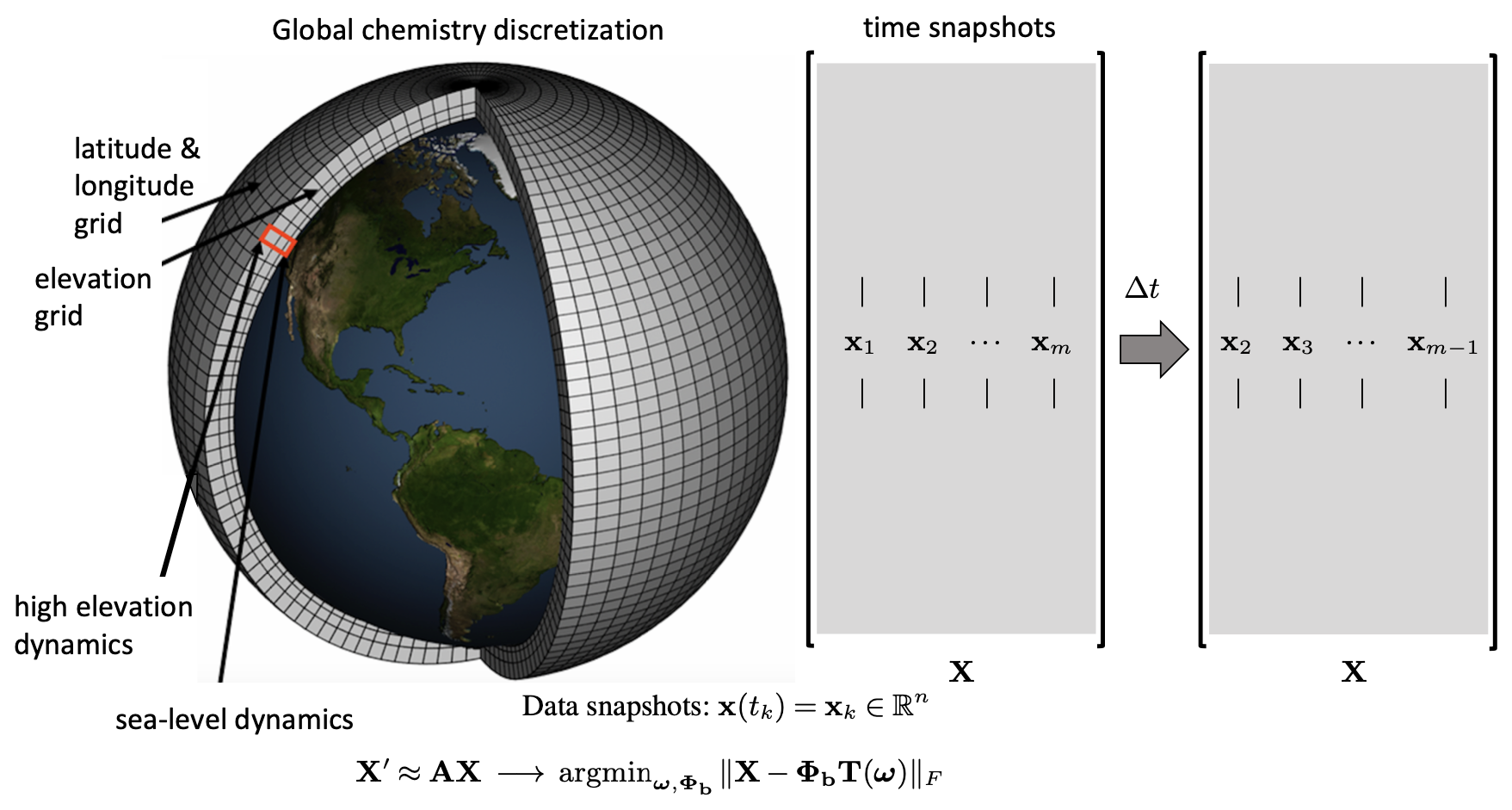
Figure 1 The spatial grid for atmospheric chemistry data sets on the left panel. The data x(t_k) are collected into snapshot matrices X, which are used to regress to the best exponential (linear) solution ${\text{argmin}}_{\mathit{\omega },{\mathrm{\Phi }}_b}\Vert \mathbf{X}-{\mathrm{\Phi }}_b\mathbf{T}\left(\mathit{\omega }\right){\Vert }_F$, where Φ_b denotes the weighted DMD modes and T fitting the data (Eq. 6).

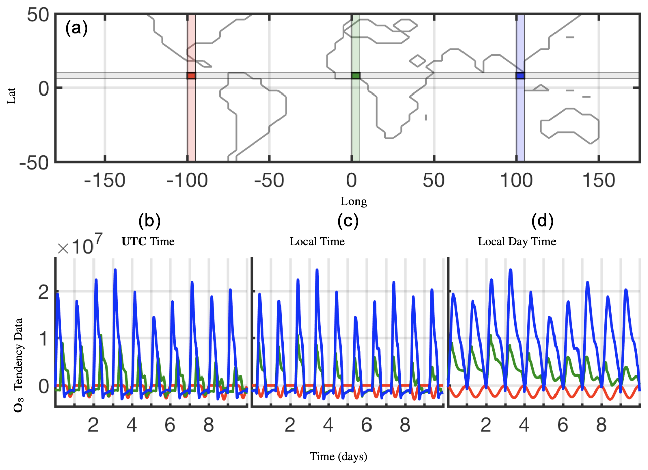
Figure 2 Shifting the data for each cell in time to align the local time zones across a latitude to the prime meridian (long=0°) local time, shown here for O₃ tendency data for lat=30°. (b) is the raw data for the three highlighted cells, (c) is those data shifted in time, and (d) shows isolated daytime values only.

However, the DMD formulated by this regression is rarely used for the forecasting and/or reconstruction of time-series data except in cases with noise-free or nearly noise-free data. This is because the exact DMD (Eq. 5) is extremely sensitive to noise in the data, causing a bias in the computed DMD modes and eigenvalues (Bagheri, 2014; Dawson et al., 2016; Hemati et al., 2017). The optimized DMD (optDMD) algorithm of Askham and Kutz (Askham and Kutz, 2018), which uses a variable projection method (Golub and Pereyra, 2003) for nonlinear least squares to compute the DMD for unevenly timed samples, provides the best and most optimal performance of any algorithm currently available. Indeed, this optimal performance is mathematically guaranteed by the exponential fitting procedure of Askham and Kutz (Askham and Kutz, 2018). The exponential fitting is given by

$$\begin{array}{}\text{(6)}& {\text{argmin}}_{{\mathit{\omega }}_k,{\mathit{\varphi }}_k,b_k}\Vert \mathbf{X}-\sum _{k=\mathrm{1}}^r{b}_k{\mathit{\varphi }}_k\exp \left({\mathit{\omega }}_{k}t\right){\Vert }_{\mathrm{2}}^{\mathrm{2}},\end{array}$$

where a rank r approximation is estimated. As noted, optimized DMD iterates to a solution of this non-convex problem by using variable projection (Golub and Pereyra, 2003). This approach has been shown to provide a superior decomposition due to its ability to optimally suppress noise bias and handle snapshots collected at arbitrary times. Figure 3 shows a comparison of surface nitrogen oxide (NO) as produced by GEOS-Chem (top panel), reconstructed using classical or exact DMD (middle panel), and generated using optDMD (bottom panel). The classical DMD reconstruction dies out within a few days, failing in the task of even reconstructing the time-series data, let alone forecasting, as it was originally regressed to. In contrast, optDMD is able to capture, sustain, and faithfully reconstruct the original time series.

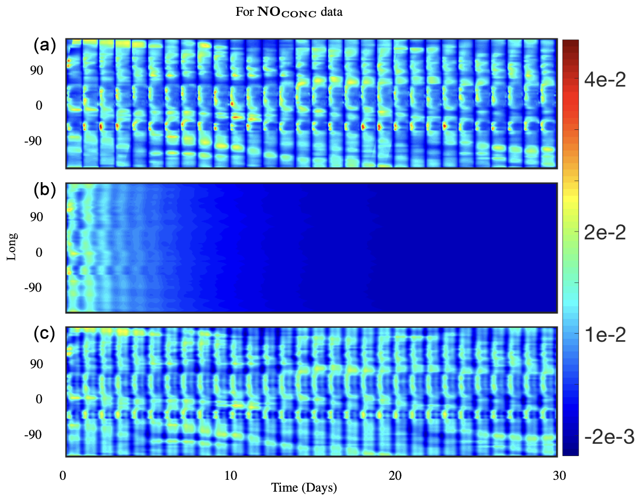
Figure 3 Comparing 30 d reconstruction results for classical and optimized DMD at the surface of NO preprocessed data at lat=30°. The results are for absolute concentration or CONC data; (a) shows the preprocessed data, (b) shows the reconstruction from classical DMD, and (c) shows the reconstruction from optimized DMD. Classical DMD is unable to capture the dynamics for the absolute concentration data, and it decays down to zero. Optimized DMD reconstructs the data and resolves the dynamics accurately.

We can also introduce constraints to the optDMD algorithm, including constraining all the DMD eigenvalues in Eq. (6) to (i) the imaginary axis:

$$\begin{array}{}\text{(7)}& \mathrm{subject}\mathrm{to}\mathrm{\Re }\left({\mathit{\omega }}_k\right)=\mathrm{0}\end{array}$$

or (ii) the closed left half-plane:

$$\begin{array}{}\text{(8)}& \mathrm{subject}\mathrm{to}\mathrm{\Re }\left({\mathit{\omega }}_k\right)\le \mathrm{0}.\end{array}$$

As discussed below, these constraints further stabilize and make robust the reproduction and forecast of the time-series data. The disadvantage of optimized DMD is that one must solve a nonlinear optimization problem through variable projection (Golub and Pereyra, 2003), which can often fail to converge.

2.4 Bagging OPtimized Dynamic Mode Decomposition (BOP-DMD)

BOP-DMD (Sashidhar and Kutz, 2022) leverages Breiman's statistical bagging sampling strategy (Breiman et al., 1984) in partnership with the optimized DMD algorithm. The BOP-DMD architecture is presented in Fig. 4. Bagging is designed to produce an ensemble of models, thereby reducing model variance and suppressing overfitting by design. Not only does ensembling improve DMD, but it is also effective in deep neural network regressions (Allen-Zhu and Li, 2020). Further innovations include stabilizing the variable projection technique used by optDMD so that it converges consistently to an optimal solution (Sashidhar and Kutz, 2022). Its ability to converge is often dependent upon a suitable initial guess for the DMD eigenvalues and eigenvectors.

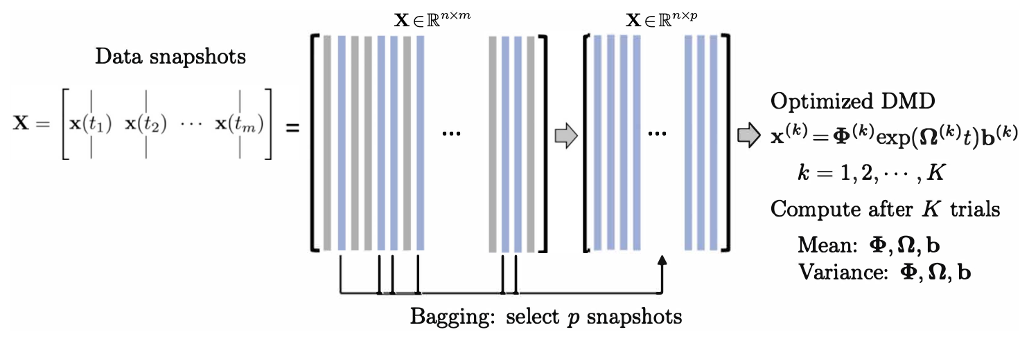
Figure 4 Summary of the BOP-DMD architecture, reproduced with permission from Sashidhar and Kutz (2022). The data snapshots x(t_k) are collected over m snapshots into the matrix X. Columns of X are randomly sub-selected into the matrix X^(k) to build an optimized DMD model. Each DMD model x^(k)=Φ^(k)exp (Ω^(k)t)b^(k) is used to compute the statistics (mean and variance) of the DMD parameterizations $\mathbf{\Phi },\mathbf{\Omega },\mathit{b}$, which are used to build the BOP-DMD ensemble solution with uncertainty quantification (UQ).

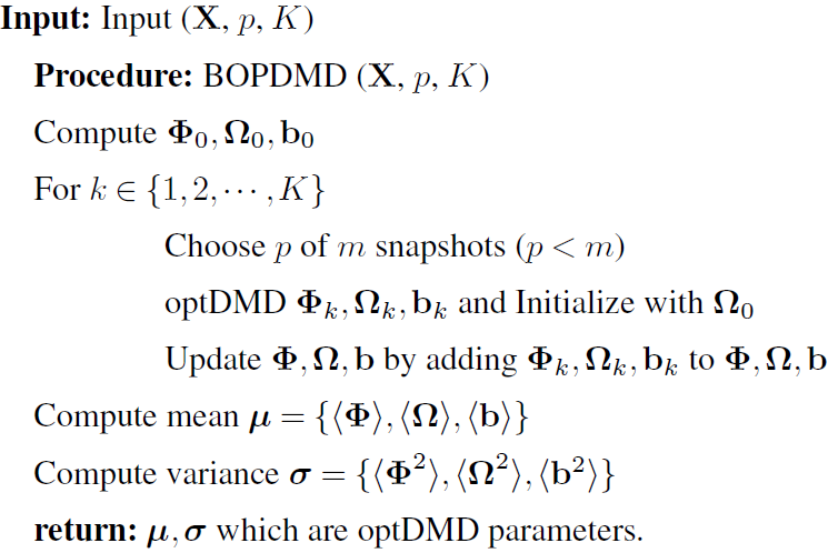
The BOP-DMD algorithm accounts for the initialization process and further provides the optimal solutions to linear models by using optDMD as the regression architecture. Algorithm 1 shows the algorithmic structure of BOP-DMD, highlighting the bagging, initialization, and ensembling of the DMD models to produce an ensemble, probabilistic DMD model. The initialization of DMD is accomplished by first constructing an optDMD model approximation, whose eigenvalues and eigenvectors Φ₀ can be used to seed the BOP-DMD. p snapshots are randomly selected from the full data matrix $\mathbf{X}\in {\mathbb{R}}^{n\times m}$ to form a subset data matrix $\mathbf{X}\in {\mathbb{R}}^{n\times p}$. optDMD produces the model for this subset data, and we save the resulting model parameters. The process is repeated for K trials, producing an ensemble of optDMD models. The mean $\mathit{\{}\langle \mathbf{\Phi }\rangle ,\langle \mathbf{\Omega }\rangle ,\langle \mathit{b}\rangle \mathit{\}}$ and variance $\mathit{\{}\langle {\mathrm{\Phi }}^{\mathrm{2}}\rangle ,\langle {\mathbf{\Omega }}^{\mathrm{2}}\rangle ,\langle {\mathit{b}}^{\mathrm{2}}\rangle \mathit{\}}$ of the model parameters $\mathrm{\Phi },\mathbf{\Omega },\mathit{b}$ can now be computed. Hence, in addition to producing the DMD model itself, the output of algorithm 1 generates both spatial and temporal uncertainty quantification (UQ) metrics. In this work, we primarily focus on the temporal UQ metrics for forecasting.

Algorithm 1 BOP-DMD.

3 Results

The analysis is performed for preprocessed or time-shifted raw data for 60 d from 2 July–30 August. This time period is characterized by very active photo-chemistry in the Northern Hemisphere. The photolysis rate dictates a different kinetic environment for many key species of interest. To simplify the interpretation, the analysis is performed on surface data (elevation =1), one latitude at a time, and for all 72 longitudes, with data shifted in time as described above.

In most of the latitudes in the Southern Hemisphere, the days are much shorter than the nights; accordingly, the daylight chemistry period is much shorter than the nighttime chemistry period. Thus, the data exhibit a spiky pattern that needs much higher modes to accurately reconstruct it, and/or we would need to isolate the daytime values only when there are active chemical kinetics present. Hence, we choose latitude =30° N for the analysis, which has the longest daytimes for the latitudes considered. The first 40 d of data are used as training data, and the DMD diagnostics below are presented for this time period and for latitude =30°. With 72 snapshots per day, we have a data matrix of 72(long)×2880(time) for each latitude. optDMD is performed for this data matrix. We perform the analysis for six different chemical species of interest (Velegar et al., 2019): nitric oxide NO, ozone O₃, nitrogen dioxide NO₂, hydroxyl radical OH, isoprene ISOP, and carbon monoxide CO. For each species, we have CONC or absolute concentration data (expressed in units of molec. cm⁻³) and TEND or tendency/rate of change data (expressed in units of molec. cm⁻³ s⁻¹). Using the diagnostics from the 40 d training period (2 July–10 August), we then forecast the chemical evolution for the following 20 d (11–30 August). The number of days used for fitting (40 d) is one of two hyper-parameters for the DMD regression, the other being the number of modes (rank) used. A sliding window approach for sampling for DMD has been shown to be quite effective for reconstruction and forecasting (Kutz et al., 2016b; Lapo et al., 2024). Typically, a shorter sampling window helps in forecasting, as the data is often non-stationary and long time histories compromise the DMD model. Thus, we use a fairly representative model history of 40 d for forecasting, which also makes the model smaller and thus easier to manage. In general, this is also in keeping with the DMD philosophy of a model that can be simply run again due to its small computational footprint. Although there are hundreds of chemicals whose dynamics can be demonstrated, the six selected are chemicals commonly associated with atmospheric diagnostics, including pollution and environmental health. Similarly, out of the large number of latitude, longitude, and elevation settings, we highlighted surface dynamics, as these are often some of the richest and most relevant for understanding the role of atmospheric chemistry affecting humans. It is an intractable task to show all chemicals at all locations. Thus, the judicious choices represent those of greatest impact and which are commonly considered by experts in practice. The code provided allows one to consider any chemical at any location desired. There are, of course, limitations to the methodology presented, especially when considering chemical dynamics that are highly intermittent and which lack any periodic or quasi-periodic behavior. Ozone is an example of a chemical that is intermittently active in its dynamics, thus compromising the ability of an algorithm like DMD to produce quality reconstructions and forecasts. Such chemicals have been excluded from consideration, as methods for such time-series behavior are currently lacking.

3.1 DMD diagnostics

The optDMD algorithm decomposes data into time dynamics represented by the spectrum of eigenvalues Ω and the corresponding spatial modes Φ. Here, we present diagnostics from four different DMD approaches: (i) optDMD without constraining the eigenvalues; (ii) optDMD with eigenvalues constrained to the left half-plane; (iii) optDMD with eigenvalues constrained to the imaginary axis; and finally (iv) exact DMD. This approach is taken to examine which decomposition is best suited for the reconstruction and forecasting of the chemistry dynamics. The constraints are important in practice, especially for forecasting the atmospheric chemistry. Without constraints, and often due to noise, the data can generate eigenvalues that have positive real parts. Even moderate-length forecasts will blow up artificially due to the real part being positive. The optDMD algorithm allows us to remove this unbounded artificial exponential growth. Growth of the solution is still accommodated by modeling it as the first part of an oscillatory solution (which looks like it is growing but is, in reality, an oscillating mode). Similarly, it has already been noted that noise can also artificially bias the eigenvalues towards the left half-plane, which makes solutions decay to zero. Thus, a forecast will exponentially die away to zero. The constraint of the eigenvalue on the imaginary axis guarantees a stable long-term forecast that neither grows nor decays. Of course, this is a pure regression problem, which induces its own limitations, but in regards to forecasting, it has the important and desirable property of stability for long-term forecasting. There is an additional inherent assumption with constraining the eigenvalues to the imaginary axis: conservation of mass of that chemical species. The diagnostics are presented for the 40 d time series of the hydroxyl radical species (OH). The results are consistent for all chemical species of interest. Specifically, the forecasting performance and error are agnostic to the specific chemical species considered, thus suggesting the DMD behavior is independent of the specific chemistry being modeled. We have used a hard rank threshold truncation of r=25 for the CONC data and r=50 for the TEND data. Truncating the rank for the DMD models is described below. These specific target ranks are chosen through hyper-parameter tuning of their forecasting performance. Too few modes compromises the DMD model because there are not enough features to accurately reconstruct and forecast the data. Too many modes causes overfitting to occur on the training data. Thus, although arbitrary, these specific values show generically strong performance across chemical species for the task of forecasting. The diagnostics are presented for both absolute concentration of the chemical species, or OH_CONC data, on the left panels and the rate of change of concentrations/tendencies due to chemistry, or OH_TEND data, on the right panels in Figs. 5 and 6. Four different spectra of the DMD eigenvalues are presented in Fig. 5, and the corresponding reconstruction of data is shown in panels 2–5 of Fig. 6. The top two panels in Fig. 6 give the actual OH_CONC data (left) and actual OH_TEND data (right), presented for comparison.

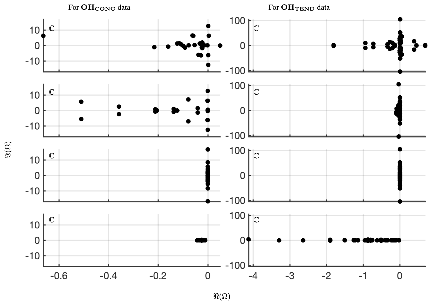
Figure 5 Comparing the spectrum for 40 d reconstruction results for classical and optimized DMD at the surface of OH preprocessed data. On the left four panels are the eigenvalues of OH_CONC data; on the right four panels are the eigenvalues of OH_TEND at lat=30°. The top panels show the spectrum from optimized DMD with no constraints, the second set of panels show the spectrum from optimized DMD with linearized constraints requiring that the eigenvalues be on the left half-plane, the third set of panels show the spectrum from optimized DMD with linearized constraints requiring that the eigenvalues be imaginary, and the bottom panels show the spectrum from classical or exact DMD. Note that a hard rank threshold truncation of r=25 for the CONC data and r=50 for the TEND data has been used.

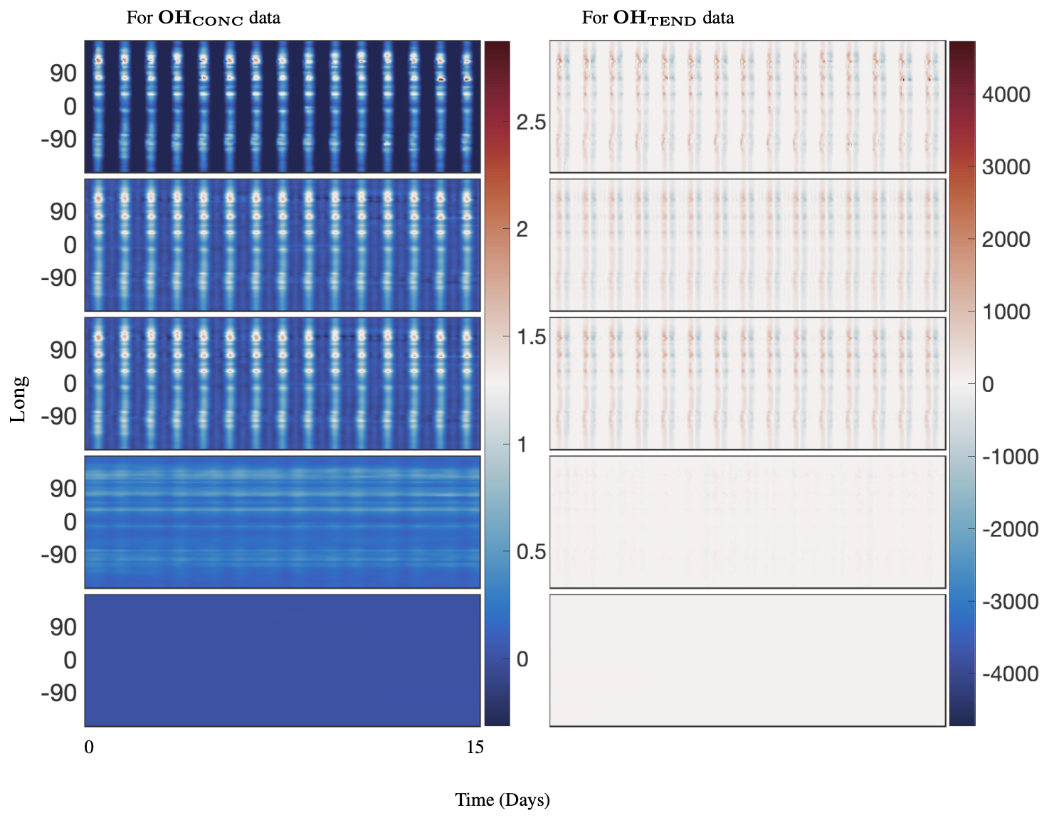
Figure 6 Comparing 40 d reconstruction results for classical DMD, optimized DMD, and optimized DMD with no constraints at the surface of OH preprocessed data at lat=30°. The left panel is for absolute concentration or CONC data, and the right panel is for Tendency data. The top panels show the preprocessed data, the second panels show the reconstruction from optimized DMD, the third panels show the reconstruction from optimized DMD with eigenvalues constrained to the left half-plane, the fourth panels show the reconstruction from optimized DMD with eigenvalues constrained to the imaginary axis, and the bottom panels show the reconstruction from classic DMD. Classic DMD is unable to reconstruct the dynamics for the absolute concentration and tendency data. Note that a hard rank threshold truncation of r=25 for the CONC data and r=50 for the TEND data has been used.

• i.

  The spectrum for optDMD with no constraints on the eigenvalues for OH_CONC data is presented in the top-left panel and for OH_TEND data is presented in the top-right panel of Fig. 5. For both data sets, some eigenvalues fall on the right half-plane with positive real parts, causing the corresponding modes to grow in time. The corresponding reconstruction of data is presented in the second two panels of Fig. 6. optDMD with no constraints does a faithful reconstruction of data, but the forecasting results are poor, with the time series growing exponentially as a result of some eigenvalues on the right half-plane. This approach is not used henceforth.

• ii.

  optDMD is then constrained to produce only eigenvalues with negative or zero real parts, i.e., eigenvalues on the closed left half-plane (ℜ(ω_i≤0)). The resulting spectrum for the two data sets is presented in the second two panels in Fig. 5. The corresponding reconstruction of data is presented in the third two panels of Fig. 6. Not only does optDMD with these constraints faithfully reconstruct the data, but the forecasting results are also accurate, as presented in the following section.

• iii.

  optDMD is then constrained to produce only imaginary eigenvalues with zero real parts (ℜ(ω_i=0)). The resulting spectrum for the two data sets is presented in the third two panels in Fig. 5. The corresponding reconstruction of data is presented in the fourth two panels of Fig. 6. optDMD with these constraints is not able to capture the data dynamics and will not be used henceforth.

• iv.

  Finally, results from exact DMD for both data sets are presented in the bottom two panels of Figs. 5 and 6. The resulting spectra for the two data sets have most eigenvalues on the negative real axis, implying decaying modes. The corresponding reconstruction of data also decays out with no dynamics from the data captured or represented faithfully. This approach is not used henceforth.

Thus, we will use optDMD with eigenvalues constrained on the closed left half-plane ℜ(ω_i≤0). When computing optDMD, we truncate the number of modes to avoid fitting dynamics to the lowest energy modes, which may cause overfitting and may be corrupted by noise. We would be truncating using hard-thresholding at a rank r at which the relative error in the reconstruction has an elbow, i.e., the error graph flattens out without further decrease. Focusing on six key chemicals of interest – $\mathrm{NO},{\mathrm{O}}_{\mathrm{3}},{\mathrm{NO}}_{\mathrm{2}},\mathrm{OH},\mathrm{ISOP},\mathrm{CO}$ – and the CONC and TEND data, we now compute the relative error as we increase the number of modes from 1 to 50. The results for the two data sets and the six chemical species are presented in Fig. 7. A larger number of modes is needed to reconstruct the TEND data compared to the CONC data. Based on the results, we use 20–30 modes for optimal diagnostics of the CONC data, depending on the chemical species. For the TEND data, we pick between 30 and 50 modes.

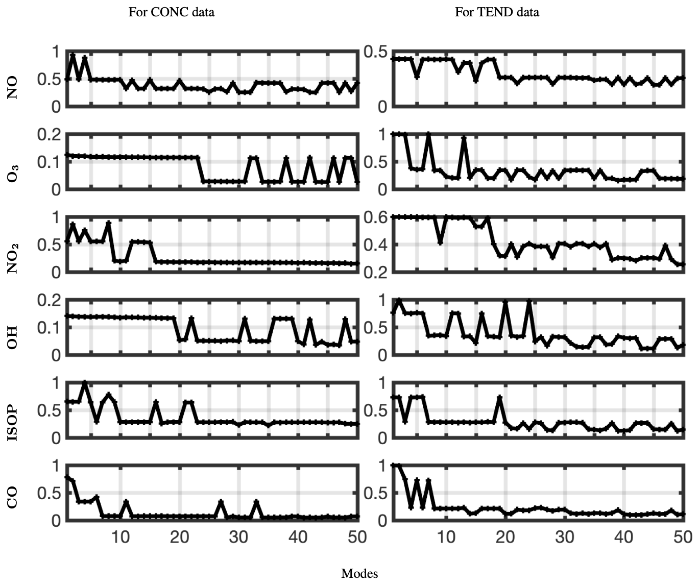
Figure 7 Relative error plotted against the number of modes used for optimized DMD with the eigenvalues constrained to the left half-plane for six different chemical species and the CONC and TEND data at latitude = 30°.

Finally, we present the global spatial modes for CO and NO, computed at 12 latitudes from −14° through 30°, in Figs. 8 and 9, respectively. The 12 latitudes are selected for having consistent day lengths across all longitudes and at least four snapshots during daytime. As described above, optDMD is performed one latitude at a time to have consistent daytime lengths across all the time series, and the resulting spatial modes are pieced together to present a global picture. The underlying spatial features of the data sets are resolved well by the constrained optDMD diagnostics. The high-variance features at the coastlines and within hot spots inland for the chemical species are represented clearly (Jacob, 1999; Brasseur and Jacob, 2017).

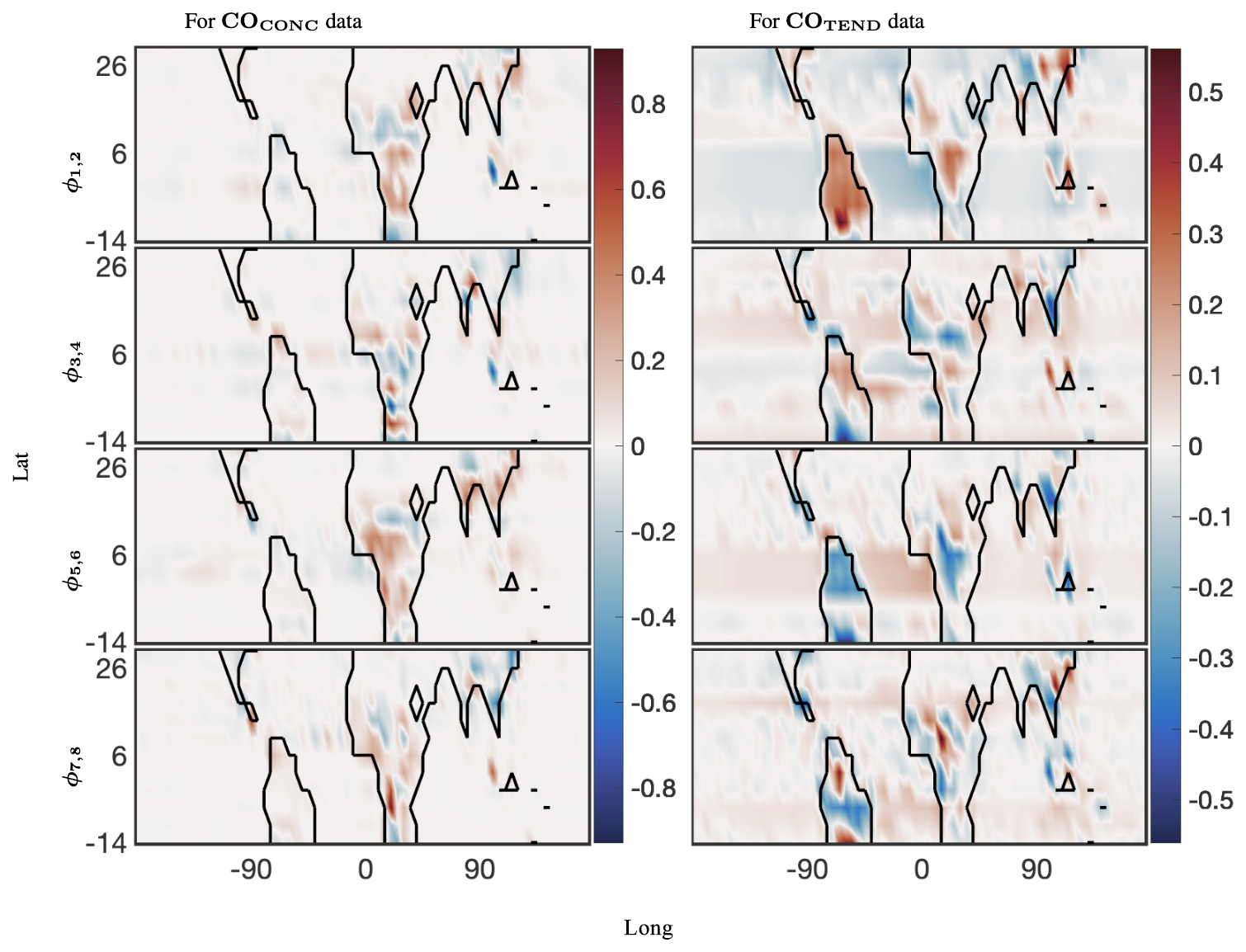
Figure 8 The 40 d reconstruction results for optimized DMD at the surface of CO preprocessed data. The analysis was computed for 12 latitudes from −14° through 30°. The left panel shows the dominant four spatial modes for the CONC data, and the right panel shows four of the corresponding spatial modes for the TEND data. The complex conjugate pair of DMD modes are denoted by ϕ_i,j, where, for the pairing, $j=i+\mathrm{1}$. Thus, ω₁ and ω₂ are the complex conjugate pairs whose real parts are identical.

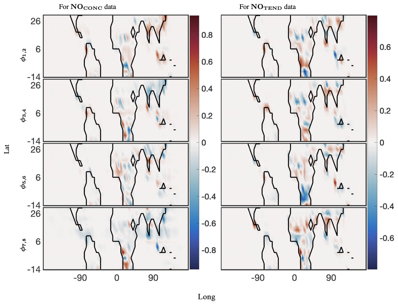
Figure 9 The 40 d reconstruction results for optimized DMD at the surface of NO preprocessed data. The analysis was computed for 12 latitudes from −14° through 30°. The left panel shows four spatial modes for the CONC data, and the right panel shows four of the corresponding spatial modes for the TEND data. The complex conjugate pair of DMD modes is denoted by ϕ_i,j, where, for the pairing, $j=i+\mathrm{1}$. Thus, ω₁ and ω₂ are the complex conjugate pairs whose real parts are identical.

3.2 Forecasting

As described above, using an appropriate rank truncation, the optDMD algorithm with eigenvalues constrained to the closed left half-plane faithfully reconstructs the time-series data for a 40 d training window and a given elevation/latitude. We now forecast the time-series data for future times beyond the training window. Using Eq. (1), with amplitudes b, modes Φ, and eigenvalues Ω computed by optDMD during the training window, we forecast time series for the subsequent 20 d. The results for the CONC and TEND data for two chemical species OH and NO are presented for six longitudes and latitude 30° at the surface (elevation = 1) in Figs. 10,  11,  12, and  13.

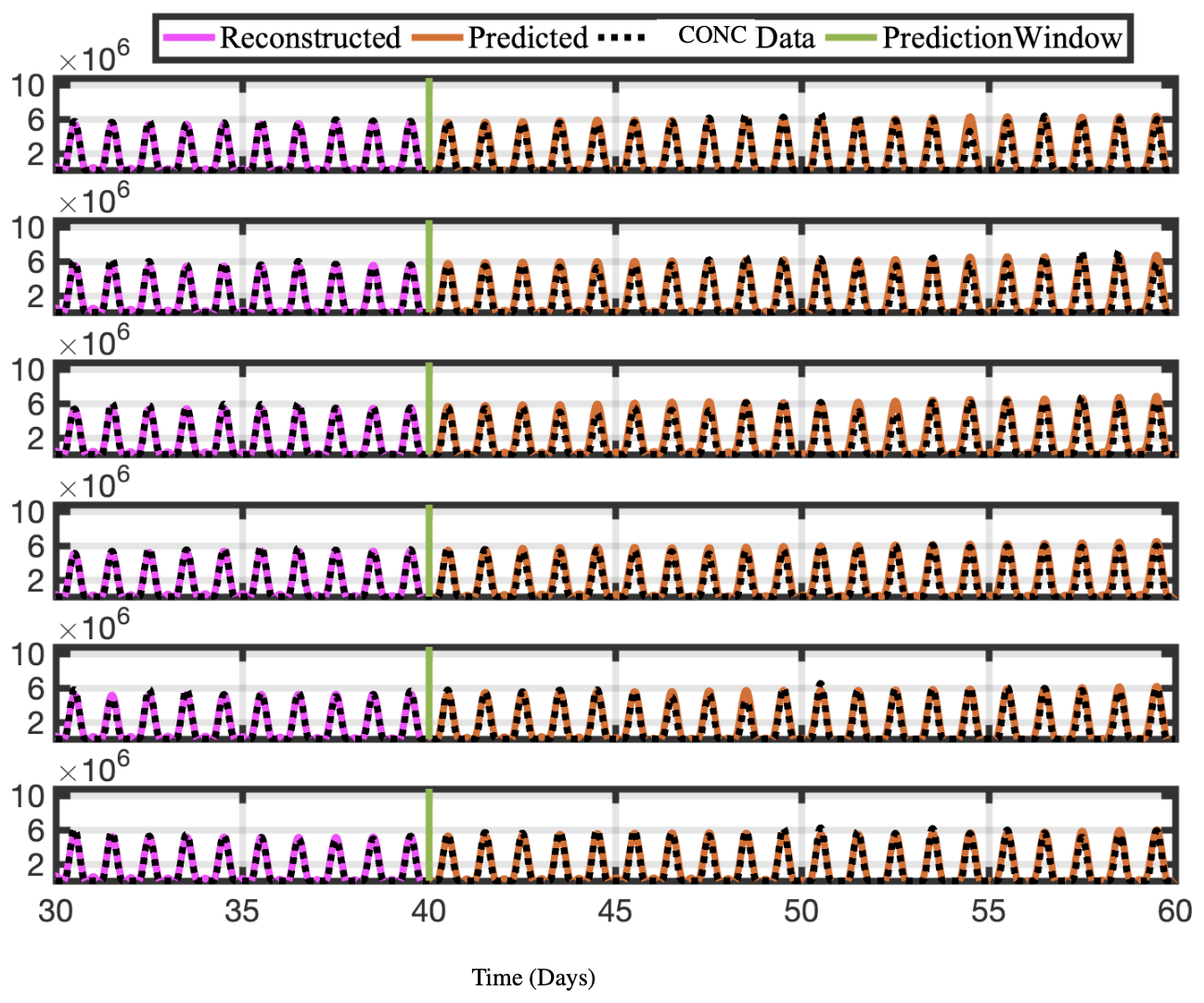
Figure 10 Time series of reconstructed and predicted results with OH_CONC data at lat =30° and six longitudes −180$\mathit{°}:\mathrm{5}\mathit{°}:-\mathrm{155}\mathit{°}$. Both the reconstructed data, shown here for 10 d, and the forecasted time series, shown here for the 20 d testing period, faithfully reconstruct and forecast the actual data for OH_CONC.

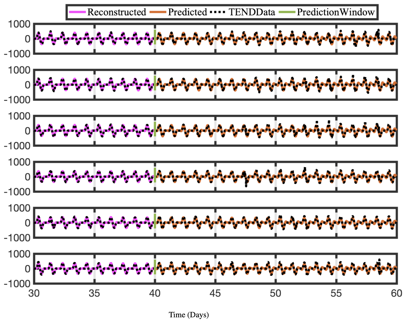
Figure 11 Time series of reconstructed and predicted results with OH_TEND data at lat =30° and six longitudes −180$\mathit{°}:\mathrm{5}\mathit{°}:-\mathrm{155}\mathit{°}$. Again, both the reconstructed data, shown here for 10 d, and the forecasted time series, shown here for the 20 d testing period, faithfully reconstruct and forecast the actual data for OH_TEND.

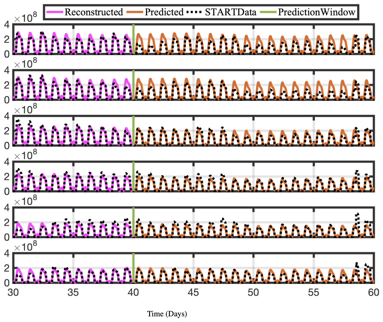
Figure 12 Time series of reconstructed and predicted results with NO_CONC data at lat =30° and six longitudes −180$\mathit{°}:\mathrm{5}\mathit{°}:-\mathrm{155}\mathit{°}$. Both the reconstructed data, shown here for 10 d, and the forecasted time series, shown here for the 20 d testing period, reproduce the actual data for NO_CONC well.

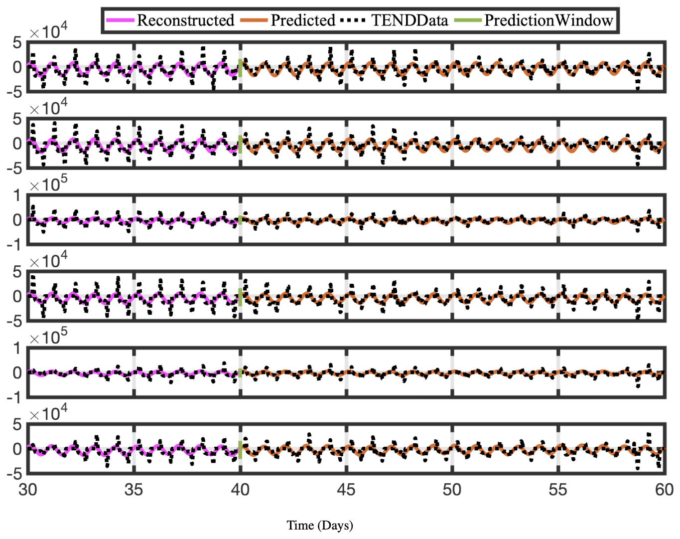
Figure 13 Time series of reconstructed and predicted results with NO_TEND data at lat =30° and six longitudes −180$\mathit{°}:\mathrm{5}\mathit{°}:-\mathrm{155}\mathit{°}$. Neither the reconstructed data, shown here for 10 d, nor the forecasted time series, shown here for the 20 d testing period, capture the spikes in the actual data for NO_TEND. Because we are using only 20–30 modes for reconstruction, we get a sinusoidal best fit. In general, spikes in time-series data are difficult to capture and forecast with any method, including DMD. Although more modes can provide a better reconstruction, it often is then overfit on training data for forecasting purposes.

Constrained optDMD faithfully reconstructs and forecasts the time series for the 20 d tested. Because we use the fewest modes possible, spikes in the actual data are sometimes not reproduced, and we see a sinusoidal best-fit time series instead. The NO_TEND results in Fig. 13 demonstrate this.

We have snapshots of the data every 20 min, hence 72 snapshots per day. We compute the relative error for all longitudes for each day and average across space and snapshots for each day. The resulting mean relative errors are presented for all six chemical species of interest and for both CONC and TEND data in Fig. 14, colored in red. The 95-percentile confidence intervals for each day are presented as black bars, indicating the variance for the mean relative errors. Constrained optDMD does an excellent job in forecasting the immediate future snapshots and does consistently well during the entire 20 d data tested, with mean errors/uncertainty in forecasting increasing only slightly for some chemical species as the number of prediction days increases away from the last snapshot used from training. No exponential growth/decay is observed in the forecast time series, while the underlying dynamics are forecast faithfully. Considering that the underlying dynamics represent a moving state with time, the constrained optDMD minimizes model bias with the variable projection optimization, thus leading to stable forecasting capabilities. The performance is slightly worse in forecasting the TEND data compared to the CONC data, which is due to the intrinsic rank of the TEND data being higher. Increasing the truncation rank of the projection would lead to an improvement in forecasting of the TEND data.

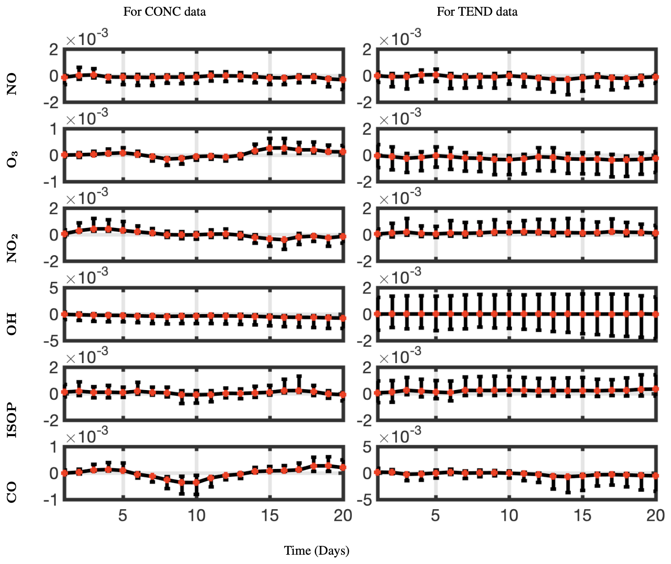
Figure 14 Mean relative error with 95-percentile confidence intervals forecasting CONC and TEND data at lat =30° for a prediction window of 20 d and for six different chemical species. The relative error stays nearly the same or changes only slightly as the number of days we are forecasting out to increases. optDMD does better at forecasting the CONC data than for the TEND data.

The optDMD algorithm performs worst in forecasting the chemical species OH. OH has a very short tropospheric lifetime of less than a second and exhibits rapid chemical cycling during the daytime. Consequently, this chemical species needs the highest number of modes to capture its dynamics (Fig. 7).

3.3 Temporal uncertainty quantification

We now present the results from BOP-DMD in partnership with the optimized DMD algorithm to produce ensemble models and compute temporal uncertainty for the eigenvalue spectrum of both the CONC and TEND data for the six chemical species of interest at lat =30°. We use the constrained optDMD as described above on a full training data set of 60 d (2 July–30 August) to create an initial seed ${\mathrm{\Phi }}_{\mathrm{0}},{\mathrm{\Omega }}_{\mathrm{0}},b_{\mathrm{0}}$ for the BOP-DMD algorithm. For K=100 trials, we randomly select p=216 snapshots/columns, i.e., data for 3 d out of the 60 d, to create our subset of data, as shown in Fig. 4. optDMD now computes the eigenvalues of various subsets using the aforementioned initial conditions. The eigenvalues for the K=100 ensemble models are used to produce the temporal UQ metrics. The UQ metrics are critical for understanding the ability of the BOP-DMD algorithm to perform long-term forecasting. Specifically, BOP-DMD is a low-cost computational tool, as opposed to Monte Carlo simulations, for evaluating the divergence of future state predictions from an ensemble of predictions, specifically drawn from the BOP-DMD eigenvalue distribution.

Figure 15 shows the BOP-DMD distributions of the absolute value of the first five eigenvalues for each of the subsets of data for OH_CONC and OH_TEND data at lat =30°. The BOP-DMD algorithm quantifies the temporal uncertainty by allowing for a Gaussian fit, shown in red. For both of the data sets, we see a high temporal uncertainty in eigenvalues, with outliers skewing the distributions. The temporal uncertainty gets worse for the higher modes in the OH_CONC data and for all modes of the OH_TEND data. Then, we trim the eigenvalue distribution data to exclude the outliers below the 10th percentile and above the 90th percentile to improve the UQ metrics. Figure 16 shows the distributions of the trimmed absolute eigenvalues, where the Gaussian fit is clearly better with lower variances, and only 1 distribution with outliers. Still, we see that there is significant temporal variability, especially for higher modes for OH_TEND.

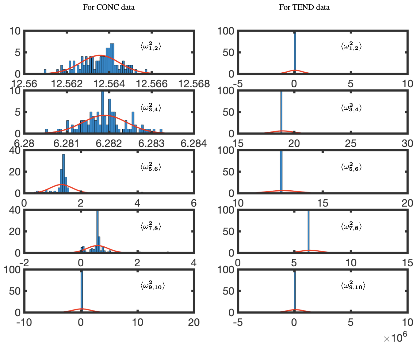
Figure 15 Temporal uncertainty quantification for absolute eigenvalues for the OH_CONC and OH_TEND data at lat =30°. The red lines represent a least-squares fit of a normal distribution; 60 d of training data was used, with a sample size of 3 d and 100 cycles. The complex conjugate pair frequencies are denoted by $\langle {\mathit{\omega }}_{i,j}^{\mathrm{2}}\rangle$, where, for the pairing, $j=i+\mathrm{1}$. Thus, ω₁ and ω₂ are the complex conjugate pairs whose variance is evaluated jointly.

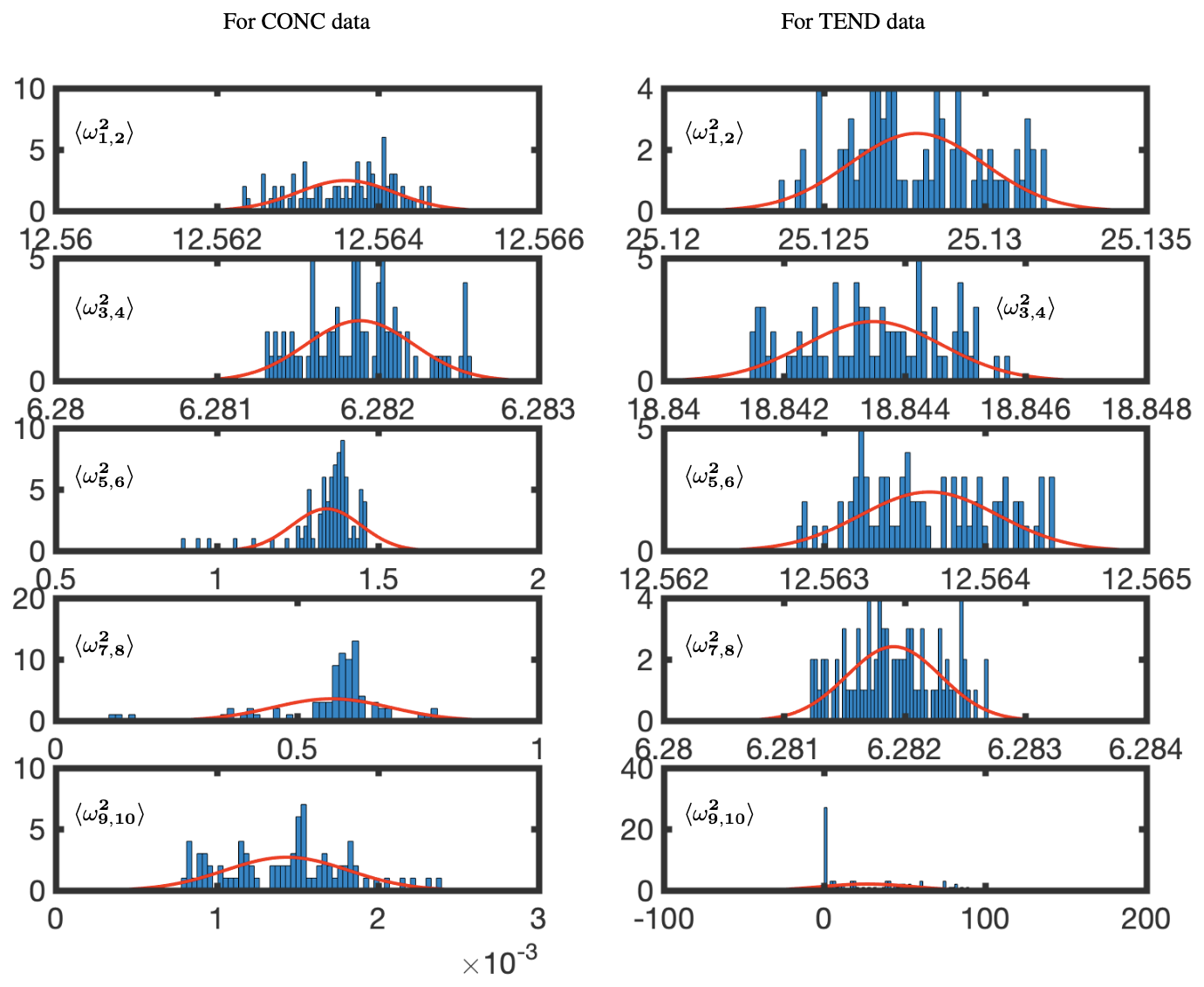
Figure 16 Temporal uncertainty quantification for absolute trimmed eigenvalues for the OH_CONC and OH_TEND data at lat =30°. The data have been trimmed to remove outliers below the 10th percentile and above the 90th percentile. The red lines represent a least-squares fit of a normal distribution. The complex conjugate pair frequencies are denoted by $\langle {\mathit{\omega }}_{i,j}^{\mathrm{2}}\rangle$, where, for the pairing, $j=i+\mathrm{1}$. Thus, ω₁ and ω₂ are the complex conjugate pairs whose variance is evaluated jointly.

4 Discussion

Based on the results presented in this work, we conclude that the constrained optDMD algorithm is the DMD algorithm of choice for the reconstruction and forecasting of global atmospheric data. Exact DMD fails in the task of reconstructing the chemistry time series it is regressed to, let alone producing a reasonable forecast. This is due to the significant bias in the model from energetic localized convective phenomena present in the atmospheric simulation data. The optDMD algorithm casts the regression problem as a nonlinear optimization enabled by variable projection techniques (Askham and Kutz, 2018), hence providing an optimal de-biasing for the atmospheric chemistry dynamics. optDMD is thus better able to capture hidden dynamics, showing an order of magnitude improvement in the reconstruction error. optDMD also produces modes that more accurately describe the localized energetic convective phenomena in the CONC and especially the TEND chemistry dynamics. The nonlinear optimization problem in optDMD also allows for constraints. By adding a constraint ℜ(ω_i≤0) to the optDMD minimization, we obtain accurate eigenvalues that are able to produce high-fidelity stable and robust forecasts. For the entire testing time window, the forecasts remain accurate as we increase time away from the training time window, not displaying any growth, decay, or loss of accuracy. However, computing optDMD requires solving a nonlinear, non-convex optimization problem, which often fails to converge to a solution. The computational cost of optDMD is higher; as we increase the number of snapshots, the cost increase becomes more significant. The solutions obtained here nevertheless represent significant improvements. Partnering the optDMD algorithm with the statistical bagging and ensembling of BOP-DMD produces temporal UQ metrics and highlights the high temporal variance in the eigenvalues produced by optDMD. This temporal variance gets worse for higher modes of the CONC data; eigenvalues for the TEND data have quite high temporal variance.

An interesting further direction would be to apply optDMD to an entire years worth of data, a still computationally tractable problem. In particular, the current study did not look at the ability of optDMD to faithfully reproduce yearly patterns in the chemistry data and accurately forecast seasonal variations. The BOP-DMD algorithm can be leveraged to produce spatial UQ metrics, illustrating the spatial patterns where optDMD is most uncertain in its ability to provide accurate representations. optDMD can be further empowered by partnering with BOP-DMD by (i) an initialization procedure to stabilize its convergence, improving the robustness and accuracy of the regression, (ii) leveraging statistical bagging to produce a stable model with reduced variance in the model parameters, and (iii) leveraging this stable model to forecast future states of a spatio-temporal atmospheric chemistry system, with Monte Carlo simulations to produce UQ for future states.

The presented approaches have the potential to produce reliable estimates of “business-as-usual” patterns of global atmospheric composition in real time and at very low computational cost. They are not designed to capture unusual events such as air pollution due to wildfires or sudden pollutant emission changes (as, e.g., experienced in the wake of the COVID-19 outbreak). However, when combined with actual atmospheric observations, the presented method can be used to identify and quantify air pollution anomalies.