SubsurfaceBreaks v. 1.0: a supervised detection of fault-related structures on triangulated models of subsurface homoclinal interfaces

The study presents a novel approach for fault detection on subsurface geological homoclinal interfaces (slopes) using a supervised learning algorithm and careful input variable (feature) selection. Synthetic faulted slopes are generated using Delaunay triangulation via the Computational Geometry Algorithms Library (CGAL), allowing for adjustments of parameters. We introduce 24 features, including local geometric features and neighborhood analysis, for classification. Support Vector Machine (SVM) is employed as the classification algorithm, achieving high precision and recall rates for fault-related observations. Application to real borehole data (elevations of buried stratigraphic contacts) demonstrates the effectiveness of the method in detecting fault orientations; the challenges remain with respect to distinguishing faults with opposite dip directions. The study highlights the need to address 3D fault zone complexities and their identification. Despite limitations, the proposed supervised approach offers significant advancement over clustering-based methods, showing promise in detecting faults of various orientations. Future research directions include exploring more complex geological scenarios and refining fault detection methodologies.

1 Introduction

Geological engineers and structural geologists aim to identify fault-related structures, as knowledge about faults is crucial in 3D geological modeling. Geological models are typically constructed by interpolating sparse (scattered) borehole data (de la Varga et al., 2019). However, due to the localized nature of boreholes, faults not directly intersected by them are often overlooked. As a result, interpolation may produce horizons that appear continuous across these faults. This paper introduces a method to detect the presence of faults under such circumstances.

Classification methods can play a crucial role in this process by helping to analyze and interpret geological data for identifying potential faults or structural features. However, current classification methods are typically tailored for seismic data rather than scattered data related to subsurface interfaces (An et al., 2021; Kaur et al., 2023). Additionally, supervised methods for fault detection can encounter challenges related to subjectivity, ambiguity, or time-consuming processes such as manual labeling of training data (Mattéo et al., 2021; Vega-Ramirez et al., 2021).

In this study, we focus on detecting faults on triangulated models of subsurface geological interfaces with preferred orientation (Fig. 1). The interfaces can be thought of as boundaries between conformal (sub-parallel) geological units or buried stratigraphic contacts often investigated in geological modeling (de la Varga et al., 2019). Data used in our study come from an irregular network of boreholes that document the transition between geological units. Consequently, the fault-related deviations from the preferred orientation are investigated using a supervised framework. In this approach, faces of the triangulation are observations described by features such as their orientation and geometric relationships with neighbors.

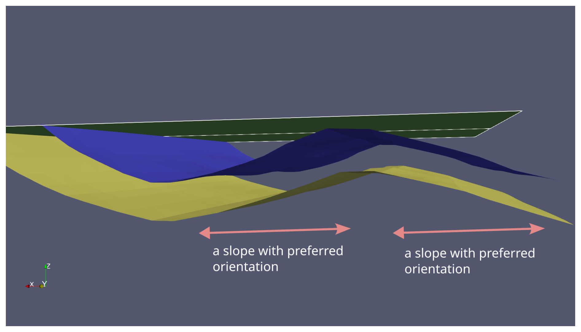
Figure 1 The supervised fault detection method developed in this study is designed for surfaces with preferred orientation (slopes). An example of such a slope can be a portion of the boundary between folded strata. The model with two folded surfaces and one erosive surface presented in this figure was generated using GemPy and GemGis software (Jüstel et al., 2022, 2023; de la Varga et al., 2019).

Our goal is to expedite the process of generating ground truth data for faulted triangulated slopes using the Computational Geometry Algorithms Library (CGAL.org, 2023). We will employ supervised machine learning algorithms for binary classification to predict possible fault presence within faulted subsurface slopes (Fig. 2). Our hypothesis posits that while traditional geometric attributes such as normal or dip vectors can still be useful for classification, integrating features reflecting angular relationships between triangles and their neighbors is crucial for accurate classification, especially for fault detection on homoclines. We assert that analyzing distances for neighbors (Fig. 3) is advantageous due to its insensitivity to surface rotation, unlike traditional geometric attributes such as dip direction (Hu et al., 2021) or the orientation of normal vectors (Michalak et al., 2022). As such, neighborhood analysis can be linked, e.g., to curvature in seismic data (de Oliveira Neto et al., 2023) in terms of its insensitivity to surface rotation.

The main challenges relate to the effectiveness of machine learning algorithms, feature selection and the applicability of the method to diverse geological structures, potentially impacting classification accuracy and generalizability. To mitigate these challenges, we will conduct optimization of the algorithm's performance and feature selection (see Methods). Validation across various geological surfaces will ensure the method's robustness and applicability for fault detection on homoclines. This structured approach aims to enhance classification accuracy and the method's utility in practical geological applications. For example, the preferred orientation of geological horizons can significantly influence groundwater flow directions in the Kraków-Silesian homocline (Razowska et al., 1997). Faults that shape the geometry of the homocline are also believed to act as barriers or preferential pathways for groundwater (Razowska et al., 1997; Razowska, 2001). The overall workflow of the study is presented in Fig. 4.

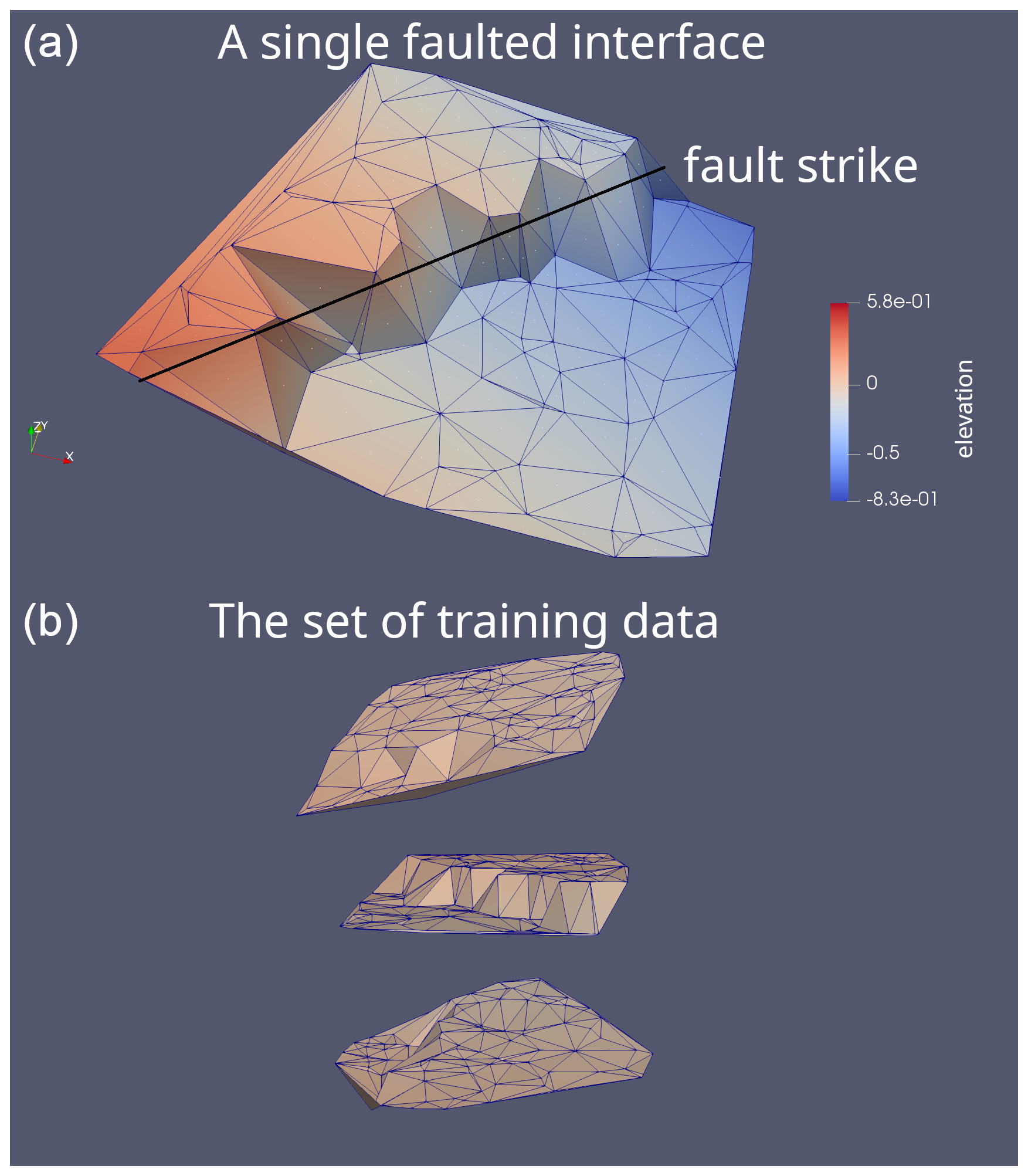
Figure 2 A triangulated model of a faulted geological subsurface interface: (a) we can see an inclined surface and triangles that intersect a fault. (b) A set of slopes with different parameters (dip angle and dip direction) can be used as training data in the classification task. In this panel, we showed only three slopes, but in practice an arbitrary number can be generated.

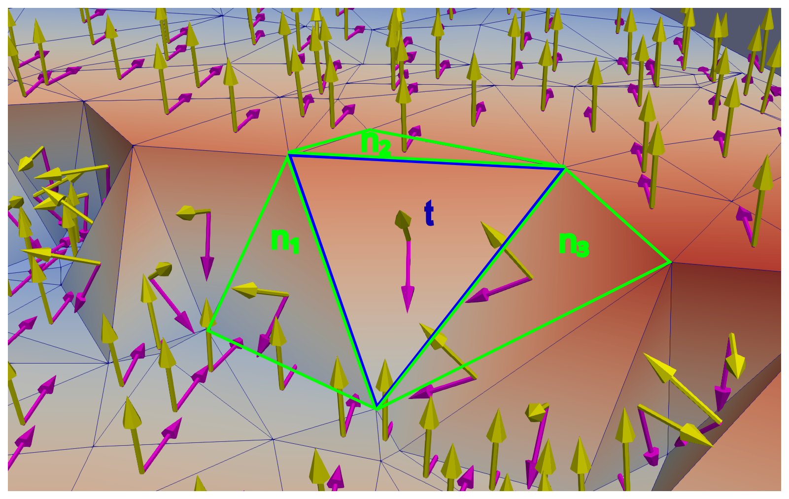
Figure 3 Because the fault introduced changes in the angular relationships between the orientation of fault-related triangles (t) and their neighbors (n1, n2, n3), the analysis of these relationships is essential for a successful classification. For example, we can measure the angular distance between normal vectors for three pairs, corresponding to a specific triangle and its neighbors. The resulting value of angular distance can serve as a feature in the classification task.

2 Background

In geological mapping, machine learning methods have been applied in the supervised lithology classification (Cracknell and Reading, 2014; Kuhn et al., 2018; Xiong and Zuo, 2021; Wang et al., 2020). In geological engineering, unsupervised methods were used to delineate subsets of observations representing discontinuities (Hammah and Curran, 1999; Zhan et al., 2017). In subsurface geological modeling, neural networks were used to delineate paleovalleys using topographic data as input data (Jiang et al., 2021), and convolutional neural networks were used to create geological models with structural features controlled by a set of random parameters (Bi et al., 2022). In the problem of fault detection, the majority of available supervised methods are primarily tailored for seismic data (An et al., 2021; Kaur et al., 2023). For topographic data, supervised methods were utilized for fault-scarp prediction (Vega-Ramirez et al., 2021) using Fisher linear discriminant analysis. However, this analysis relied on high-resolution bathymetric data based on a small training data set (163 samples). Another example involves the use of topographic attributes such as DEM, slope, aspect and faults and environmental features such as vegetation and climate for monitoring of ground deformation (Hu et al., 2021).

In the study of triangulated models of geological surfaces (Michalak et al., 2022), one of the unsupervised learning methods such as the k-means algorithm generates partitions comprising geometrically similar observations (Choi et al., 2014). However, the unsupervised methods place the burden on the user to determine whether a specific observation represents a fault. This can pose challenges, as some anomalous orientations may be associated with other structures or measurement errors. Moreover, applying unsupervised learning to 3D orientations reveals sensitivity to the choice of vectorial representation (Michalak et al., 2022), resulting in varying clustering results for dip and normal vectors.

3 Methods

In this section, we present our fault detection method, starting with the general description of Support Vector Machines for the classification. We detail the workflow, including the integration of features and geometric attributes such as the local orientation and the relationships with neighbors. Then, we describe the generation of synthetic data for model training and the final evaluation on real data. The stages of the method are summarized in Figs. 4 and 5.

3.1 Support Vector Machine

Several classification algorithms are available in the scikit-learn library (Pedregosa et al., 2011), which can be tested in terms of classification success metrics. However, in this study, we work with a single algorithm to keep focus on the new classification method. We selected the Support Vector Machine, a two-class classifier, which is considered a suitable tool for binary classification problems in high-dimensional spaces (Bishop, 2006; Vapnik, 2000) and which performed well in terms of precision and recall in our preliminary research. The Support Vector Machines algorithm can be considered an optimization algorithm because the decision is based on a hyperplane with the maximum margin. The margin is defined to be the minimal distance between a point in the training set and the hyperplane. The motivation behind the concept of margin is that if a margin is large, then it will be capable of separating the training set even after small perturbation of the instances (Shalev-Shwartz and Ben-David, 2013). Formally, the optimization objective is as follows (Bishop, 2006):

$$\begin{array}{}\text{(1)}& \arg \mathit{\left\{}\left[t_n\left({\displaystyle \frac{{\mathit{w}}^{T}f\left(x_n\right)+b}{\left|\left|\mathit{w}\right|\right|}}\right)\right]\mathit{\right\}},\end{array}$$

where $t_n\in \left\{-\mathrm{1},\mathrm{1}\right\}$ denotes the target values, and f(x) denotes a fixed feature-space transformation. This transformation is expected to facilitate separation of instances which were not linearly separable in the original space. Common choices of transformations (kernel functions) include linear, polynomial and radial basis functions. Next, w is the vector of weights which determines the orientation of the decision surface, and b is the bias parameter (not to be confused with bias in the statistical sense). The expression $\left(\frac{{\mathit{w}}^{T}f\left(x_n\right)+b}{\left|\left|\mathit{w}\right|\right|}\right)$ denotes the perpendicular distance of a point x_n to the decision surface $y\left(x\right)={\mathit{w}}^{T}f\left(x\right)+b=\mathrm{0}$. This decision surface separates points with different labels: −1 and 1. The multiplication t_ny(x_n) visible in the optimization task filters solutions for which all data points are correctly classified, i.e. t_ny(x_n)>0 . We note that in some formulations of the optimization problem, the vector of weights has unit length (Shalev-Shwartz and Ben-David, 2013). Because all N points lie beyond the margin area, they are at some distance from the hyperplane corresponding to the size of the margin. While the distances of N points relative to the decision boundary can be different, they are all greater than a fixed number, corresponding to the size of the margin which can be expressed by a set of N inequalities. Therefore, the optimization objective (Eq. 1) together with the set of N inequalities forms a constrained optimization problem which can be solved be using the Lagrange multipliers (Bishop, 2006 – Appendix E).

In the presence of outliers, a soft margin classifier can be applied, which allows some samples to be classified incorrectly (Shalev-Shwartz and Ben-David, 2013). For the soft margin classifier and radial basis function kernel, C and gamma parameters are considered. The parameter C, common to all SVM kernels, is a penalty parameter: a low C tends to make the decision surface simple (thus, avoiding overfitting but possibly affecting the correct classification of the training data), while setting a high C will result in classifying training examples more correctly (possibly leading to poorer generalizability). Gamma defines the radius of the similarity of a single training sample. The lower gamma is, the greater the similarity radius of a sample (Pedregosa et al., 2011).

We use the following metrics as evaluation metrics:

$$\begin{array}{}\text{(2)}& \begin{array}{rl}\text{precision}& ={\displaystyle \frac{\text{true positive}}{\text{true positive+false positive}}}\\ & \text{and}\text{recall}={\displaystyle \frac{\text{true positive}}{\text{true positive+false negatives}}}.\end{array}\end{array}$$

The definition implies that precision is maximized if there are no false positives and the recall is maximized when there are no false negatives. Based on these definitions the harmonic mean of both can be defined as follows:

$$\begin{array}{}\text{(3)}& F_{\mathrm{1}}=\mathrm{2}\cdot {\displaystyle \frac{\mathrm{1}}{\frac{\mathrm{1}}{\text{precision}}+\frac{\mathrm{1}}{\text{recall}}}}=\mathrm{2}\cdot {\displaystyle \frac{\text{precision}\cdot \text{recall}}{\text{precision+recall}}}.\end{array}$$

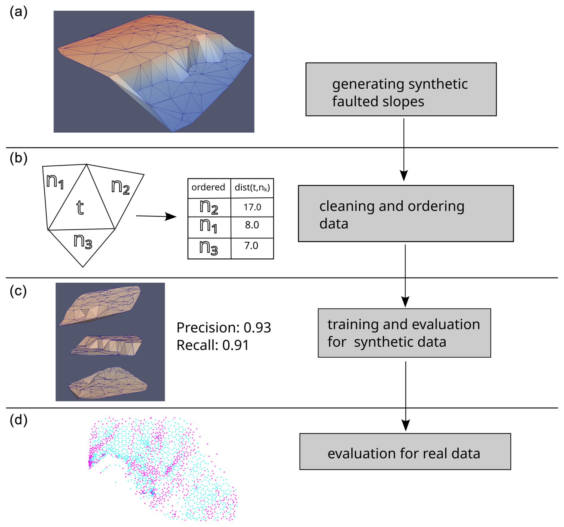
Figure 4 Workflow applied in this study: (a) we create 1000 random faulted geological slopes controlled by random parameters. (b) Then, for each triangle, we sort the distances between neighbors to reduce randomness (see Sect. 3.2 for a more detailed explanation). (c) In the next step, we train and test the machine learning algorithm for synthetic data. (d) At the end of the procedure, we evaluate the proposed approach for real data to test generalizability.

3.2 Selecting meaningful and consistent features

In this study, to predict the correct label (label = 1 for fault-related observations and label $=-\mathrm{1}$ for non-fault-related observations), we used 24 features (the features are denoted as x in Sect. 3.1). The set consists of six local geometric features and 18 features corresponding to the neighborhood analysis. The first group consists of coordinates of normal and dip vectors.

In fact, there can be even more geometric features used for the purpose of classification such as dip angle or dip direction (Hu et al., 2021; Wang et al., 2021). However, including dip direction for classification as a value within the [0, 360] range may not always be successful. This is because northern directions indicate great numerical difference (e.g. $\mathrm{358}-\mathrm{2}=\mathrm{356}$) but very small geometric difference (4°). Sometimes the limitations of using dip direction are acknowledged, and the feature is removed from the analysis (Yang et al., 2023). Therefore, in this study we did not use dip direction as a feature for classification. The second group includes features corresponding to the neighborhood component of the analysis and the set of features is as follows: angular distance, Euclidean distance and cosine distance applied to both normal and dip vector representations of the adjacent triangles. The formulas for angular (d_a), Euclidean (d_e) and cosine distances (d_c) are given in the below equations, respectively:

$$\begin{array}{}\text{(4)}& d_{\mathrm{a}}\left(u,u^{\prime }\right)=\mathrm{acos}\left({\displaystyle \frac{\mathrm{|}\mathit{u}\cdot {\mathit{u}}^{\prime }\mathrm{|}}{\mathrm{|}\mathrm{|}\mathit{u}\mathrm{|}\mathrm{|}\cdot \mathrm{|}\mathrm{|}{\mathit{u}}^{\prime }\mathrm{|}\mathrm{|}}}\right),\end{array}$$

where ⋅ is the dot product, and ||u|| is the length of the vector u. In our case, the vectors have unit length. The use of absolute value in the numerator reflects the use of acute angles between vectors.

$$\begin{array}{}\text{(5)}& {\displaystyle }{d}_{\mathrm{e}}\left(\mathit{u},{\mathit{u}}^{\prime }\right)=\mathrm{|}\mathrm{|}\mathit{u}-{\mathit{u}}^{\prime }\mathrm{|}\mathrm{|}\text{(6)}& {\displaystyle }{d}_{\mathrm{c}}\left(\mathit{u},{\mathit{u}}^{\prime }\right)=\mathrm{1}-\mathit{u}\cdot {\mathit{u}}^{\prime }\end{array}$$

However, in relation to the proposed neighborhood analysis, an obstacle arises in processing these data due to the lack of a clear distinction between first, second and third neighboring triangles (Figs. 3, 4b). This lack of order introduces randomness or arbitrariness into the analysis and compromises the consistency of data processing, which is crucial for the accuracy and reliability of the results.

To address this, we sort the distances to neighboring triangles in decreasing order. Sorting these values eliminates randomness from the analysis and ensures consistency in data processing, thereby enhancing the correctness and credibility of the results. From a technical viewpoint, the features are represented by columns in a data frame, and sorting the distances introduces their rearrangement.

3.3 Generation of training data

In our study, the synthetic training data consist of triangulated models of subsurface interfaces using the Delaunay triangulation (De Berg et al., 2008). A user has the flexibility to adjust parameters of the resulting data set in the following fields: the number of files to generate, the lower and upper bound of slope sizes, the left and right range of the dip direction, the lower and upper bound of the dip angle, the lower and upper bound of the number of points in the triangulation, the lower and upper bound of the surface noise, and the lower and upper bound of the fault throw. The user-defined parameters and their admissible ranges are specified in Table 1. However, if a constant value of a parameter should be investigated, it is possible to set the same value for the lower and upper bound. In the next step, tools from the C$++$ random number library generate random numbers from the uniform distribution using the bounds entered by a user. The information about parameters is saved to a text file to allow further inspection.

The faulted triangulated models of subsurface slopes are created in the following sequence, which is also summarized in Fig. 5 (numbers 1–6 below correspond to letters e–f in Fig. 5).

1. A container with 2D points is generated within a square of a given size.

2. A new container of 3D points is created with the Z coordinate corresponding to the random value of dip and dip direction (ranges specified by a user).

3. Noise is introduced to the surface, defined as a random fraction (ranges specified by a user) of the elevation difference within the slope.

4. A fault is introduced with the throw, defined as a random fraction (ranges specified by a user) of the maximum elevation difference within the generated slopes. The orientation of the fault is determined by two points randomly selected from the boundary of the square.

5. Triangulation of the slope is performed, and the attributes including relationships with neighbors are calculated.

6. Classification task involves labeling each observation based on whether it is a fault-related observation (label =1) or not (label $=-\mathrm{1}$). Therefore, we use the intersection predicate (CGAL.org, 2023) to test whether a specific triangle intersects the line representing a fault.

Following this approach, we are capable of generating a great number of synthetic and labeled ground truth data.

The parameters used in this study are given in the Table 2. To ensure that the training is performed on good-quality data, we removed triangles with a high degree (0.90 and greater) of collinearity, defined as a ratio between the longest triangle's edge and the sum of remaining lengths (Michalak, 2018). This coefficient lies in the interval [0.5, 1], with lower and higher values pointing to equilateral and collinear configurations, respectively (Michalak et al., 2021; Michalak, 2018).

Table 1 Input parameters. The parameters given in the table are specified by the user by providing ranges. To generate a single model, a number from the uniform distribution is drawn using the provided ranges. Please note that dip angle and dip direction are not used directly in the later stages as features for classification but first are converted into normal and dip vectors.

Table 2 Values or ranges for parameters used in this study.

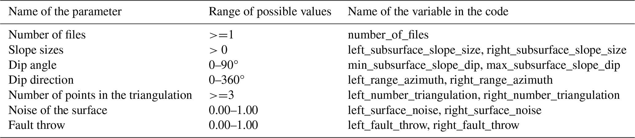
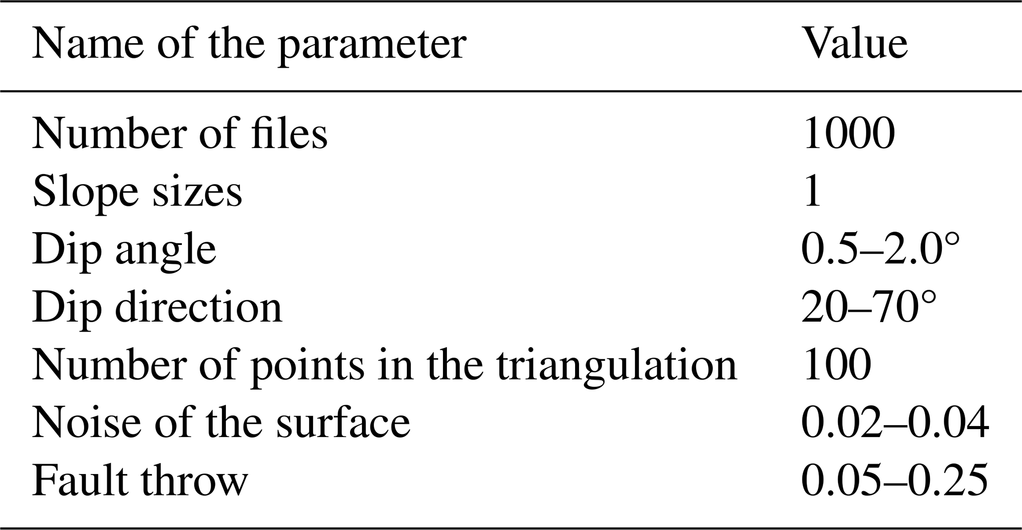
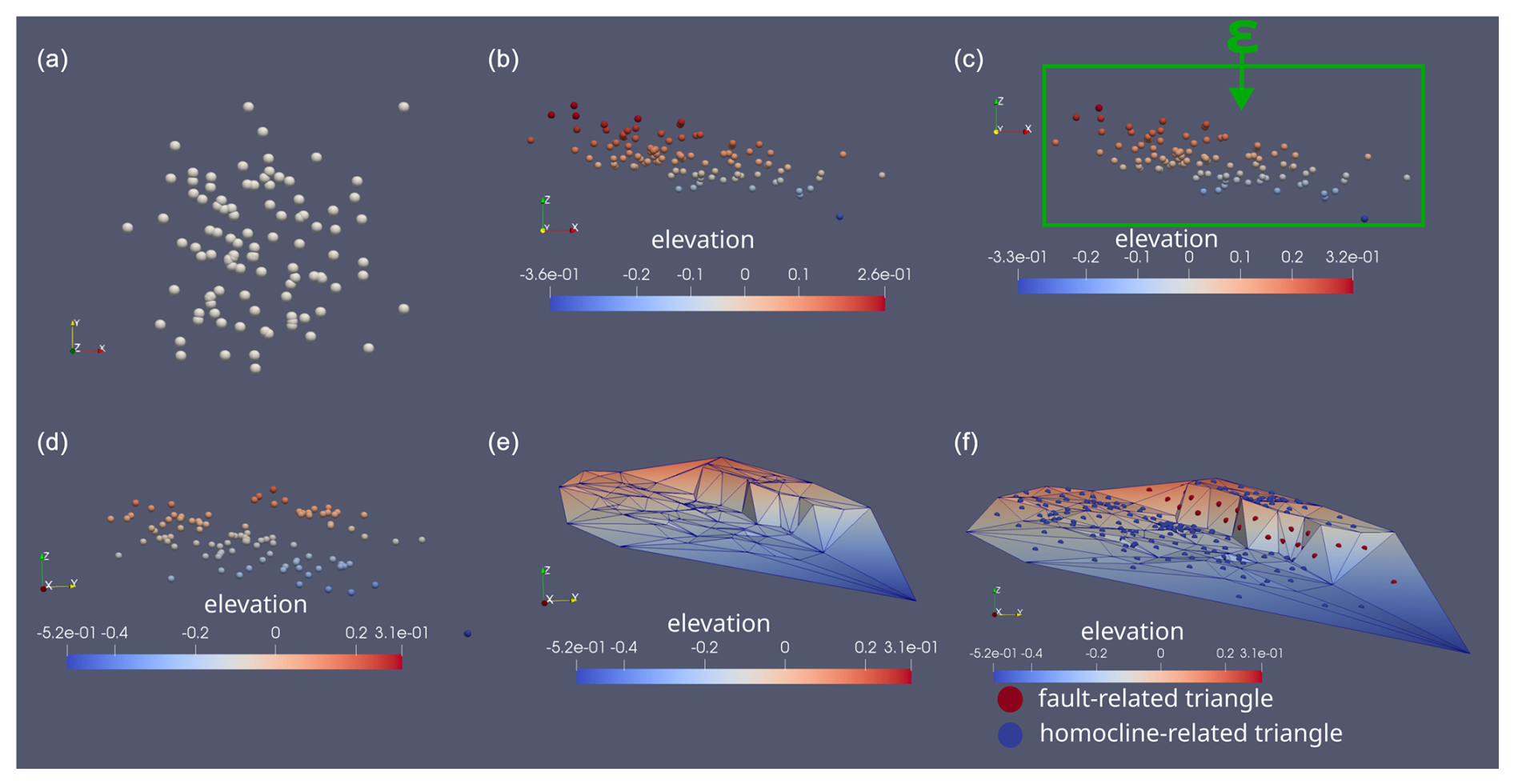
Figure 5 Depiction of sequence of processes applied to generate training data: (a) creating points in 2D space, (b) assigning elevation to the data depending on the randomly generated dip angle and dip direction, (c) adding noise (ε) to the data, (d) introducing faults and resulting elevation changes, (e) applying triangulation to the data and (f) labeling the data according to the location relative to the fault plane.

3.4 Spatial clustering

In our study, we visualize the classification results for real data using the concept of spatial clustering (Fisher, 1993; Fisher et al., 1985). The definition of spatial clustering is first studying the directional information of the data without taking into account spatial information. This study aims to group geometrically similar observations, and at the end the resulting clusters of directions are put back into their spatial context (Fisher, 1993). Indeed, in our case the Support Vector Machine algorithm performs the classification ignoring spatial information. It only uses geometric information such as the orientation of a triangle and the relationships between a triangle and its neighbors. The labels of clusters grouping similar triangles are recorded initially as integers corresponding to fault-related triangles (label = 1) or triangles belonging to the homocline (label $=-\mathrm{1}$). Then, the integers are converted to colors and presented on a map receiving again spatial information. As Fisher (1993) notes, the spatial clustering is somewhat paradoxical: “to perform the desired directional-spatial clustering, it may be necessary to decouple the directional from the spatial information initially”.

4 Geological setting (corresponding to real data)

4.1 Regional and geometric background

As a relevant case study, we selected Kraków-Silesian Homocline (KSH) – a geological structure considered to be a limb of the Szczecin-Łódź-Miechów Synclinorium. The formation of KSH is mainly attributed to the inversion of the Permian–Mesozoic Polish Basin (Dadlez et al., 1995; Słonka and Krzywiec, 2020). From a geometric perspective, KSH dips at low angles to NE (Matyszkiewicz et al., 2015). Several attempts have been made to quantify this orientation:

• dip angle <2° with NE dip direction (Znosko, 1960; Marynowski et al., 2007),

• 2–5° with NE dip direction (Bardziński et al., 1986),

• 0.98–1.35° as lower and upper bounds for dip angle with 53.47–54.86 as left and right bounds for dip direction; these values were calculated as mean orientation corresponding to the cluster associated with regional trend using two variants of hierarchical clustering (Michalak et al., 2019)

It is generally assumed that the faults form a unimodal set of sub-parallel faults trending NE–SW (Fig. 6a, Hermański, 1993; Więckowski et al., 1985). However, later clustering experiments with two or three clusters (Michalak et al., 2022) added knowledge about geometric anomalies also aligned with the N–S direction (Fig. 6b, c). To investigate generalizability of the proposed method for real data, we used borehole data (Michalak, 2024) corresponding to a horizon separating Middle Jurassic rock units: Aalenian–Early Bajocian Kościeliska sandstones from Late Bajocian–Late Bathonian ore-bearing clay deposits (Matyja and Wierzbowski, 2000; Kopik, 1998).

4.2 Discussion of previous results

Little is known about faults trending perpendicular to the preferred dip direction. While the results (Fig. 6b, c) suggest that they may not exist, we note that this negative effect could be due to limitations of unsupervised learning methods: the spatial distribution of labels depends on the partition induced by clustering algorithms. This dependence may result in visual disintegration of rare structures represented by observations being in different clusters. For example, the boundary between blue and purple labels may be related to faults dipping to SW (Fig. 6). Likewise, it is unlikely that all observations dipping to NE are genetically related to the homocline; instead, observations dipping to NE but with a dip angle greater than that of the homocline may be related to faults dipping to NE.

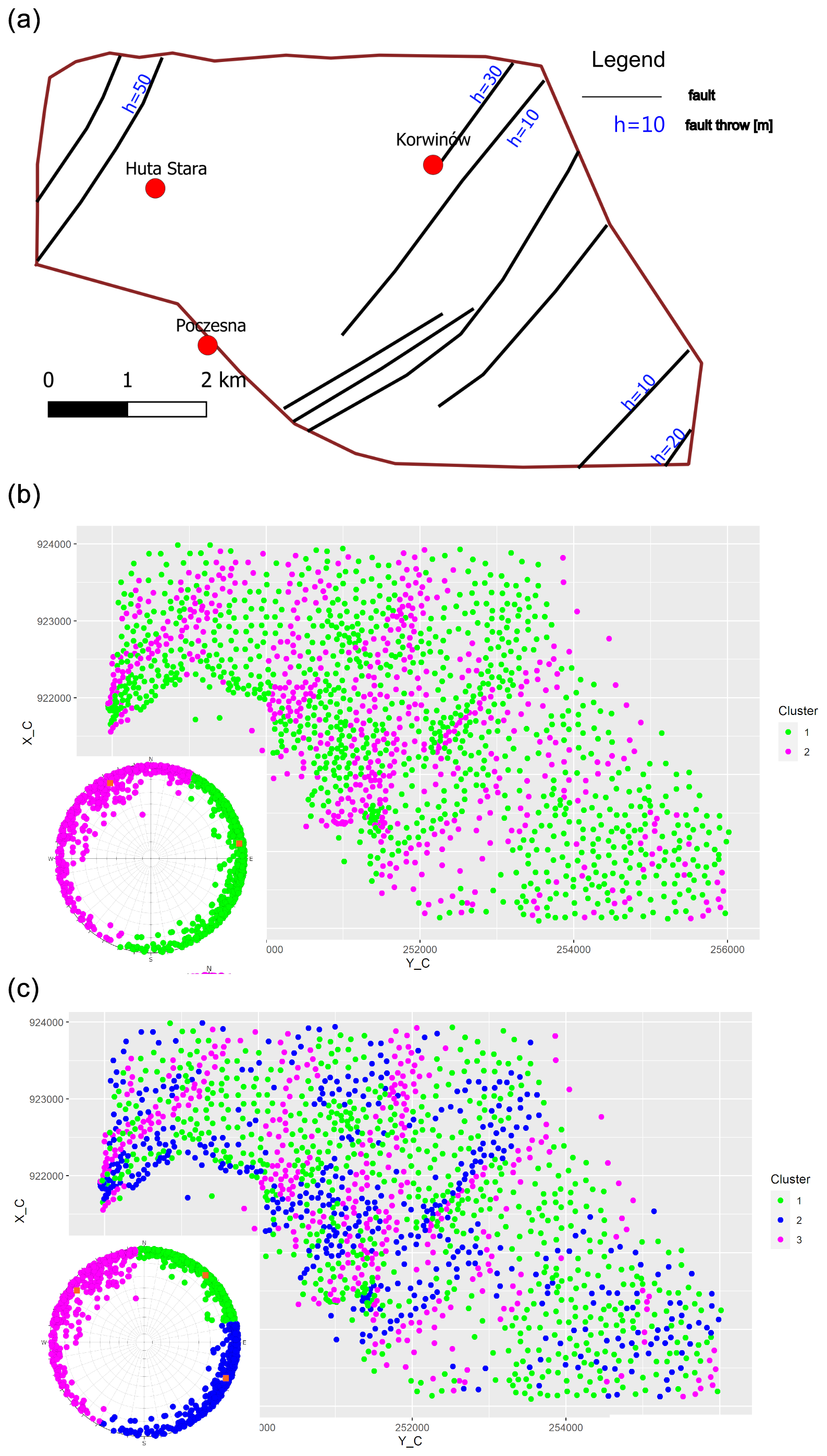
Figure 6 Progressing knowledge about tectonics of the Kraków-Silesian Homocline. (a) Due to abandoned mining activity in the area, it was possible to confirm some of the faults and their properties such as fault throw in underground mines (Hermański, 1993). Later experiments based on cluster analysis (k-means algorithm, Michalak et al., 2022) of normal and dip vectors provided evidence about the orientation of geometric anomalies. (b) Clustering of dip vectors for two clusters. The spatial distribution of labels suggests presence of geometric anomalies trending from S–N to SW–NE. (c) Clustering of dip vectors for three clusters. The spatial distribution of labels in the NW part of the study area suggests presence of more than one fault trending SW–NE with opposite dip direction. However, the partition induced by the clustering makes it impossible to identify faults dipping to NE steeper than the homocline. Data used to generate labels in panels (b) and (c) are borehole data (buried stratigraphic contacts) used in this study, as well. The figure is a modified figure from using unsupervised classification of triangulated models of borehole data used in this study (Michalak et al., 2022).

5 Results

5.1 Synthetic data

In our study, we used 1000 triangulated interfaces (slopes) with 100 points in every slope (see also Table 2). This configuration resulted in the initial number of 185 980 triangles. We removed collinear configurations (collinearity > 0.90) and triangles which did not have three finite neighbors. As a result, 145 297 triangles remained. And only a small fraction of triangles are fault-related triangles (12 411 vs 132 886). Therefore, to reduce class imbalance, we randomly select 12 411 observations from the class with non-fault observations. Taking all considerations into account, we have 24 822 samples with 12 411 observations for each class (−1 and 1). Then, the set was divided into a training (18 616) and test (6206) set.

For arbitrarily selected hyperparameters (C = 0.05, gamma = 0.042), with radial basis function as kernel function) in the scikit-learn framework, we achieved the confusion matrix for the test data as shown in Table 3.

Table 3 Confusion matrix for the classification task before hyperparameter tuning. The sum of the entries is equal to the number of samples in the test data.

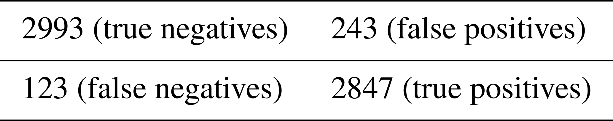
The values of precision and recall for the fault-related observations are 0.92 and 0.96, respectively (Table 4). However, the arbitrarily selected hyperparameters are not guaranteed to give the best performance of the algorithm. To further increase the values of the classification metrics, we tested many combinations of the hyperparameters as a part of the grid search optimization (Pedregosa et al., 2011). The grid is defined by the following values of parameters: 0.1, 1, 10, 100, 1000 (for C), 1, 0.1, 0.01, 0.001, 0.0001 (for gamma) and “rbf” with “linear” (for kernel). These values were selected to cover a wide range of potential hyperparameter settings during grid search optimization. The optimal combination of hyperparameters turned out to be as follows: C=10, gamma = 0.01 with radial basis function as the kernel function. The classification results change slightly after the grid optimization stage (Tables 5 and 6).

Table 4 Results for the classification of test data (unseen slopes) for arbitrarily selected hyperparameters (before hyperparameter tuning).

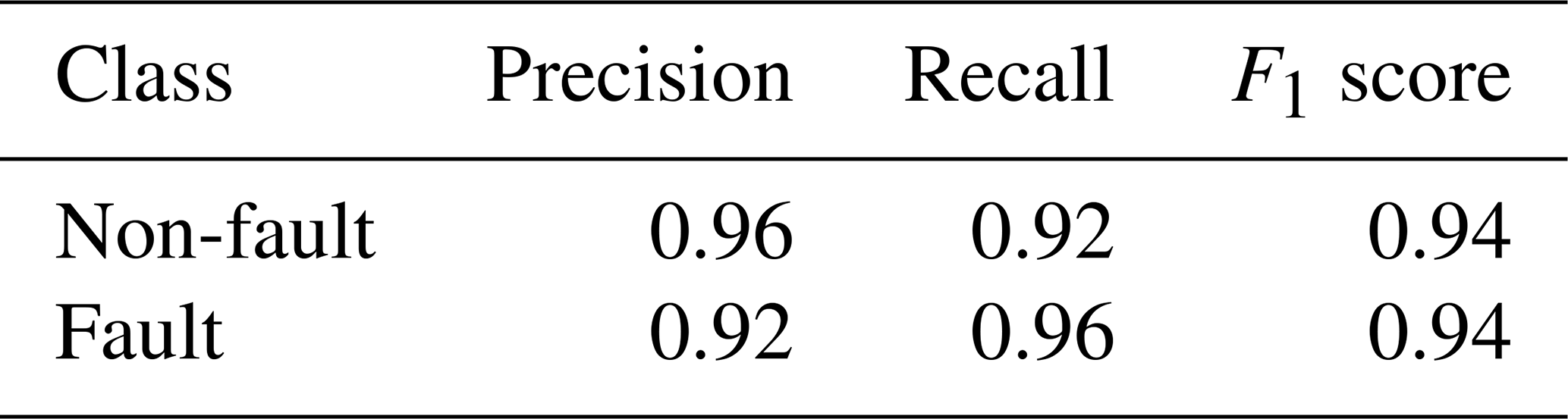
Table 5 Confusion matrix for the classification task after hyperparameter tuning. The sum of the entries is equal to the number of samples in the test data.

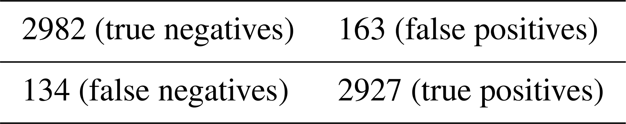
Table 6 Results for the classification of test data (unseen slopes) after the fine tuning of the hyperparameters during grid search optimization.

5.2 Real data

The results of supervised classification using SVM are similar to those obtained using unsupervised (Michalak et al., 2022) classification (compare Figs. 6 and 7) in that the majority of faults have the SW–NE, SSW–NNE or S–N orientation. However, there are significant differences which relate to visibility of new potential faults trending perpendicular to the preferred dip direction. For example, Fig. 7a in the central part (near coordinates 921500, 251000) shows two potential faults trending NW–SE at the termination of S–N and SSW–NNE-trending potential faults. Another difference is that the unsupervised classification presented the major fault in the NW part of the study area as possibly composed of smaller faults with opposite dip direction (Fig. 6c, near coordinates 922000, 248500). In contrast, the binary classification cannot distinguish between faults with opposite dip directions. Therefore, the zone of fault-related labels near the discussed fault zone appears relatively wide.

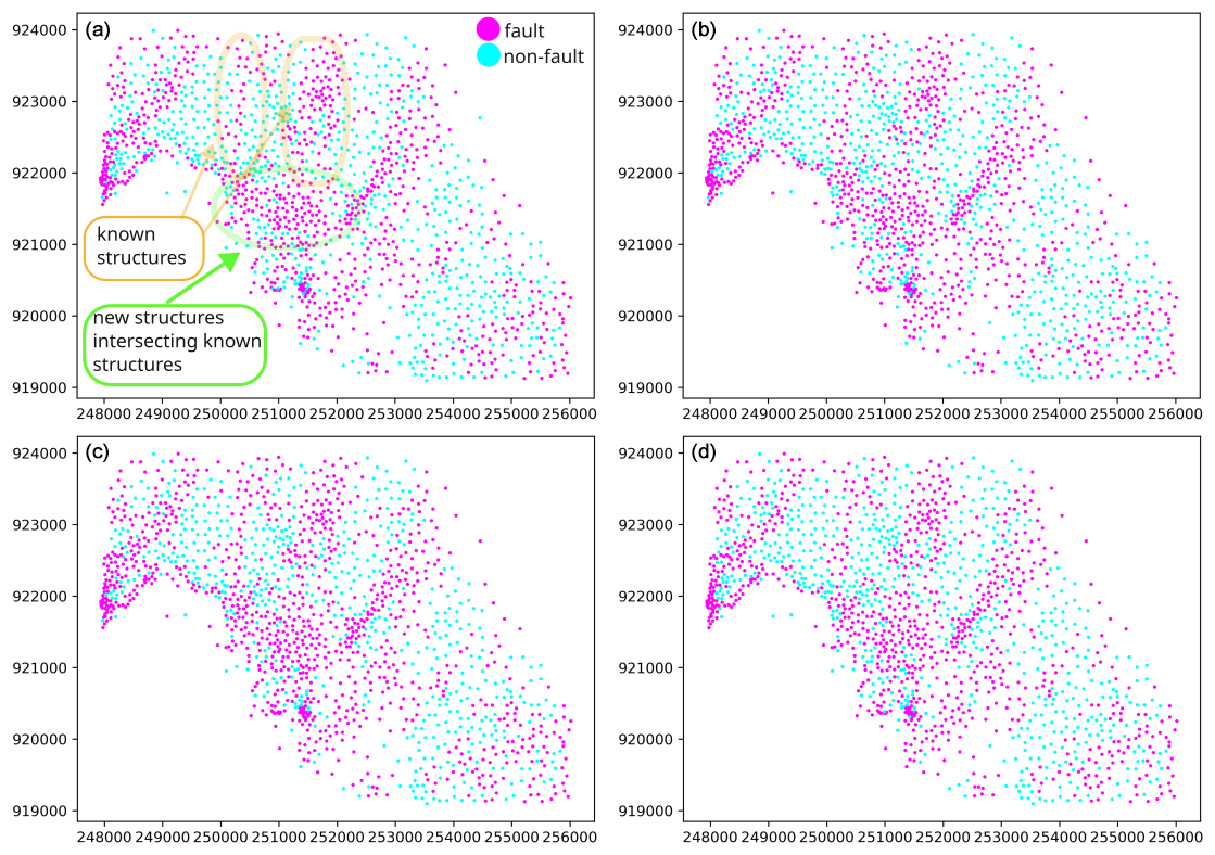
Figure 7 Classification results for the Kraków-Silesian Homocline: (a) the optimal combination of the hyperparameters as suggested by the grid search optimization (C=10, gamma =0.01, with radial basis function as the kernel function), (b) a custom combination of the hyperparameters (C=1, with linear kernel), (c) a custom combination of the hyperparameters (C=10, with linear kernel) and (d) a custom combination of the hyperparameters (C=10, gamma = 0.01, with the radial basis function as the kernel function). In panel (a), we marked structures known from the unsupervised learning revealed in previous studies (Michalak et al., 2022). The new structures revealed in this study using the supervised classification and the area where both groups intersect are marked, as well.

6 Discussion

6.1 Advantages of using faces of triangulation

In our study, we used local geometric attributes of triangles and neighborhood analysis to predict faults on triangulated models of subsurface slopes representing buried stratigraphic contacts. In subsurface geological modeling, the neighborhood analysis was already applied for individual boreholes of triangulated surfaces to analyze connectivity of strata (Guo et al., 2024). From a viewpoint of graph theory, in our case the neighborhood analysis is performed on finite faces of the triangulation rather than on its finite vertices (boreholes). Because, for every triangulation, with k being the number of points on the edge of the convex hull, the relationship between vertices (n) and triangles (m) is $m=\mathrm{2}n-\mathrm{2}-k$ (De Berg et al., 2008), our approach will usually (except very small data sets) result in a greater number of observations compared to a potential approach of considering boreholes as observations. Moreover, our approach ensures that every observation has three finite neighbors, which testifies that observations are comparable. When neighbors of points are considered, this is not the case because the degree of a vertex usually is not a constant number.

6.2 Comparison with unsupervised approaches

The improvement of the supervised approach over the unsupervised method (Michalak et al., 2022) is that the clustering results depend on the partition generated by clustering algorithms. Therefore, the unsupervised version offers to examine spatial distribution of clusters. But it does not offer the examination of spatial distribution of structures related to different clusters. Moreover, the empirical results showed that clustering algorithms often struggle to separate regional trend from faults striking perpendicular to the regional trend on homoclines (Fig. 6b, c). Therefore, the solution of the binary classification task obtained in this study could also have implications for previous research regarding the calculation of the regional trend (Michalak et al., 2019). In that study, the regional trend was calculated by averaging the orientation of triangles classified within the most numerous cluster. However, this cluster also included triangles with dip angles steeper than those characteristic of the homocline, which could have influenced the accuracy of the calculated regional trend. Compared to the unsupervised method (Fig. 6c, the NW part of the study area), the main drawback of the supervised approach is that the algorithm cannot distinguish between different dip directions of a fault. Therefore, a zone of fault-related labels may consist of many sub-parallel sequences of labels corresponding to more than one sub-parallel faults possibly with opposite dip direction (Fig. 7, the NW part of the study area).

6.3 Complexities of real data

The borehole data set documenting the interface between Kościeliska sandstones and ore-bearing clays has been traditionally used for inferring tectonics (Znosko, 1960). However, it should be admitted that there is a hiatus covering the earliest Late Bajocian, confirmed by the lack of Strenoceras subfurcatum Ammonite Zone (Garbowska, 1978). It is unclear whether some of the identified structures (Fig. 7) can be attributed to erosion. For example, some researchers point out that erosion took place during the earliest Late Bajocian (Dayczak-Calikowska and Moryc, 1988). However, some underground observations did not confirm deviations from the general parallelism between older Kościeliska sandstones and younger ore-bearing clays. Moreover, the orientation of the interface separating Kościeliska sandstones from ore-bearing clays was assumed to be uniformly inclined to the northeast in hydrogeological models during exploitation (Hermański, 1971).

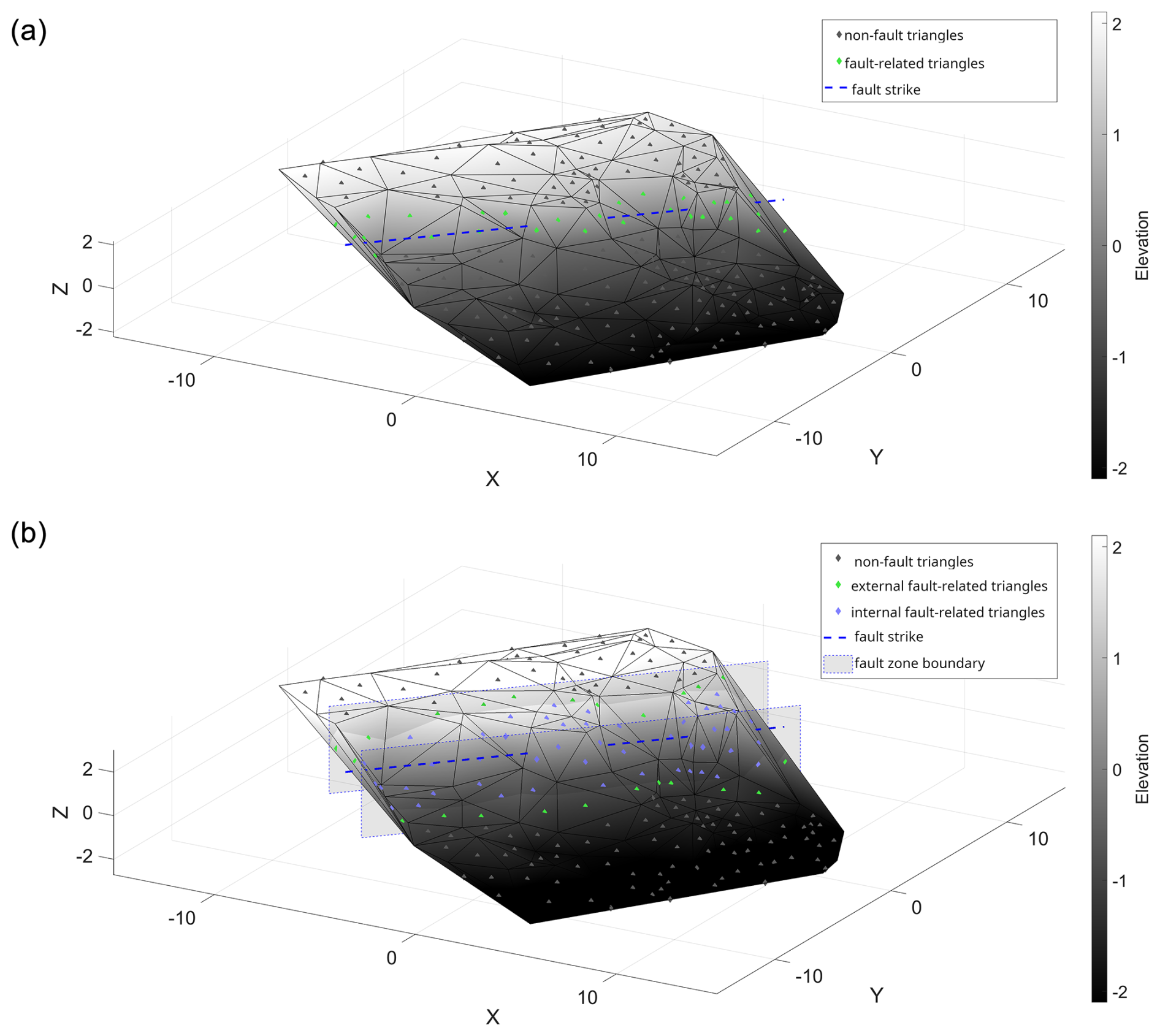
Figure 8 (a) Example of a slope generated as explained in Sect. 3.3, with the fault being represented by a plane. (b) Example of a slope generated as explained in Sect. 3.3 with the extended fault zone. Triangles with green markers show at least one non fault-related triangle as a neighbor. Triangles with blue markers only have fault-related triangles as neighbors. Grey planes represent the border of the extended fault zone.

6.4 Modeling assumptions

The main assumption for generating the triangulated models of surface data (Sect. 3.3) is that the interfaces are homoclinal (Singleton and Gans, 2008), which can correspond to limbs of folded stratigraphy. Therefore, the proposed tool should be used with caution in areas near fold hinges or limbs with opposing dip directions. It appears that the orientation of normal or dip vectors allows the orientation of only one limb to be constrained, posing a risk that non-faulted limbs could be misidentified as faulted. We hypothesize that the neighborhood component of the analysis, which is not sensitive to rotation, could potentially extend the applicability of the method. However, confirming or rejecting this hypothesis would require additional data, particularly from regions containing small-scale folds.

Another major assumption is that a fault is always represented by a vertical plane. In our case, we assume that any surface point lies either on one or on the other side of the fault, and it is not possible that any surface point is located on the fault. When these surface points are triangulated, each fault-related triangle connects points from both sides of the fault. Every fault-related triangle has at least one neighbor that is not associated with the fault. The fault is represented by a stripe of the fault-related triangles (see triangles with green markers in Fig. 8a).

This main assumption is a simplification. In reality, a fault structure is never a purely planar object. It is mostly a 3D structure that has an extension perpendicular to the fault strike (Childs et al., 2009). Therefore, it is possible that at least some surface points may be located inside the fault zone. When triangulating these points, there is the possibility to create fault-related triangles, all of whose neighbors are fault-related triangles as well (see Fig. 8b, triangles with violet markers).

These “internal fault-related” triangles show a combination of patterns that was never trained. Triangles that exhibit patterns that were actually trained are still present (see Fig. 8b, triangles with green markers) but are only located at the borders of the fault zone (grey rectangles in Fig. 8b). This leads to the assumption that the presented classification system may classify the extended fault zone not by one sequence of color-coded labels but by two quasi-parallel sequences of this type. Whether the “internal fault-related triangles” can be successfully classified is an open question. In terms of local geometric features specific to a single triangle such as coordinates of normal vectors, the “internal fault-related” triangles are more similar to the classical fault-related triangles. In contrast, the neighborhood analysis alone would likely classify these triangles as non-fault-related triangles (triangles with grey marker in Fig. 8a and b). A comprehensive answer to this question would require additional experiments or substantial modifications of modeling assumptions (introducing non-vertical faults in the training), which lies beyond the scope of our research.

The influence of 3D fault zones for the classification result needs to be further studied. Nevertheless, in the context of this study the data points are assumed to be sparsely scattered. If the fault shows an extension significantly lower than the mean data point spacing, the simplified assumption of purely planar faults is valid. The problem of identifying internal fault triangles could possibly be ameliorated by including not only the direct neighbors of a triangle in the training procedure but also triangles that are second- or third-degree neighbors or neighbors with an even higher number of degrees. Using this approach, it is more likely that the extended neighborhood of an “internal fault-related” triangle also contains non-fault-related triangles. However, the concept of the suggested approach would stay the same. For illustration purposes we, therefore, stick to the simplest setup.

7 Conclusions

In this study, we developed a supervised fault detection method for triangulated models of subsurface slopes representing buried stratigraphic contacts. The novelty lies in generating a large number of synthetic slopes using the CGAL library and their triangulated models using Delaunay triangulation. The orientation of individual triangles combined with geometric relationships with neighbors is used as features for classification. The proposed supervised method has the potential to identify fault-related structures of any orientation, which can be considered improvement over unsupervised classification approaches. The main challenge of the workflow is to eliminate arbitrariness in feature selection in relation to neighborhood analysis. Sorting distances among neighbors eliminates arbitrariness from the analysis, but it is also the most computationally intensive part of the workflow. We believe that the classification approach can be used by geologists interested in geological complexity of subsurface environments with limited availability of data. Further studies can focus on considering more complex geological scenarios, including the influence of 3D fault zones and physics-based models (compare with Conclusions in Reichstein et al., 2019).