the Creative Commons Attribution 4.0 License.
the Creative Commons Attribution 4.0 License.
 | 15 Jul 2025
DECIPHeR-GW v1: a coupled hydrological model with improved representation of surface–groundwater interactions
Yanchen Zheng
Gemma Coxon
Mostaquimur Rahman
Ross Woods
Saskia Salwey
Youtong Rong
Doris E. Wendt
Groundwater is a crucial part of the hydrologic cycle and the largest accessible freshwater source for humans and ecosystems. However, most hydrological models lack explicit representation of surface–groundwater interactions, leading to poor prediction performance in groundwater-dominated catchments. This study presents DECIPHeR-GW v1 (Dynamic fluxEs and ConnectIvity for Predictions of HydRology and GroundWater), a new surface–groundwater hydrological model that couples a model based on hydrological response units (HRUs) and a two-dimensional gridded groundwater model. Using a two-way coupling method, the groundwater model component receives recharge from HRUs, simulates surface–groundwater interactions, and returns groundwater levels and groundwater discharge to HRUs, where river routing is then performed. Depending on the storage capacity of the surface water model component and the position of the modelled groundwater level, three scenarios are developed to derive recharge and capture surface–groundwater interactions dynamically. Our coupled model was set up at 1 km spatial resolution for the groundwater model, and the average size of the surface water HRUs was 0.31 km2. The coupled model was calibrated and evaluated against daily flow time series from 669 catchments and groundwater level data from 1804 wells across England and Wales. The model provides streamflow simulation with a median Kling–Gupta efficiency (KGE) of 0.83 across varying hydro-climates, such as wetter catchments with a maximum mean annual rainfall of 3577 mm yr−1 in the west and drier catchments with a minimum of 562 mm yr−1 in the east of Great Britain, as well as diverse hydrogeological conditions including chalk, sandstone, and limestone. Higher KGE values are found in particular for the drier chalk catchments in southeast England, where the average KGE for streamflow increased from 0.49 in the benchmark DECIPHeR model to 0.7. Furthermore, our model reproduces temporal patterns of the groundwater level time series, with more than half of the wells achieving a Spearman correlation coefficient of 0.6 or higher when comparing simulations to observations. Simulating 51 years of daily data for the largest catchment, the Thames at the Kingston River basin (9948 km2), takes approximately 17 h on a standard CPU, facilitating multiple simulations for model calibration and sensitive analysis. Overall, this new DECIPHeR-GW model demonstrates enhanced accuracy and computational efficiency in reproducing streamflow and groundwater levels, making it a valuable tool for addressing water resources and management issues over large domains.
- Article
(8448 KB) - Full-text XML
-
Supplement
(2625 KB) - BibTeX
- EndNote


Groundwater systems are a vital component of the hydrologic cycle, connecting recharge zones and discharge and facilitating complex interactions between the surface and subsurface (Kuang et al., 2024; Gleeson et al., 2016; Giordano, 2009). As the main freshwater storage component of the hydrologic cycle (Aeschbach-Hertig and Gleeson, 2012), groundwater systems support baseflow levels in rivers (Miller et al., 2016; Gleeson and Richter, 2018) and provide key water supplies for industry, agriculture, and public use, especially during droughts (Famiglietti et al., 2011; Siebert et al., 2010; Giordano, 2009). As such, they are a critical resource for people, economies and the environment (Loaiciga and Doh, 2024) and play a vital role in water management. Often, groundwater models support groundwater management decision-making at the local (Wang et al., 2019; Wendt et al., 2021a), national (Dobson et al., 2020; Lee et al., 2007), continental (Rama et al., 2022; Condon and Maxwell, 2015), and global scales (De Graaf et al., 2019; Turner et al., 2019; Gorelick and Zheng, 2015).
Groundwater systems and their interactions with surface water form an active component of the hydrologic water cycle, which can have significant effects on climate, surface energy, and water partitioning (Gleeson et al., 2021; Kuang et al., 2024). The importance of representing surface–groundwater interactions in hydrological models is widely acknowledged (Gleeson et al., 2021; Condon et al., 2021; Bierkens et al., 2015; Clark et al., 2015), especially under the influence of climate change and intense anthropogenic activities (Benz et al., 2024; De Graaf et al., 2019; Condon and Maxwell, 2019). Neglecting these important surface–groundwater interactions may lead to unrealistic partitioning of precipitation between runoff and other water balance terms, such as significant evapotranspiration biases (Famiglietti and Wood, 1994; Condon and Maxwell, 2019), causing inaccurate prediction of the hydrologic states and fluxes (Naz et al., 2022; Wada et al., 2010). Gnann et al. (2023) demonstrated strong disagreement among many models in describing groundwater recharge, indicating potential errors in estimating the contribution of groundwater to evapotranspiration and streamflow. Moreover, many hydrological models across regions and countries globally struggle to reproduce streamflow dynamics in groundwater-dominated catchments (Massmann, 2020; Coxon et al., 2019; Badjana et al., 2023; McMillan et al., 2016; Lane et al., 2019; Hartmann et al., 2014) due to either oversimplified groundwater processes (Yang et al., 2017; Guimberteau et al., 2014; Gascoin et al., 2009) or complex groundwater components that are challenging to calibrate at large scales (Maxwell et al., 2015; Ewen et al., 2000; Naz et al., 2022), leading to difficulties in predicting and managing water resources in these regions.
To counter these problems, there has been a growing interest in integrating groundwater models into hydrological models, accompanied by notable progress in groundwater modelling analysis and evaluation at various scales (Gleeson et al., 2021; Condon et al., 2021). A variety of coupled surface–groundwater models has emerged across different scales (summarized in Table S1 in the Supplement). Examples at the regional scale include SWAT-MODFLOW (Bailey et al., 2016), TopNet-GW (Yang et al., 2017), mHM-OGS (Jing et al., 2018), CWatM-MODFLOW (Guillaumot et al., 2022), GSFLOW-GRASS (Ng et al., 2018), JULES-GFB (Batelis et al., 2020), SHETRAN (Ewen et al., 2000), CLSM-TOPMODEL (Gascoin et al., 2009), CaWaQS3.02 (Flipo et al., 2023), ORCHIDEE (Guimberteau et al., 2014), and HydroGeoSphere (Ala-Aho et al., 2017; Brunner and Simmons, 2012); at the continental scale, they include models such as ParFlow (Maxwell et al., 2015) and ParFlow-CLM (Naz et al., 2022); and at the global scale, models like GLOBGM (PCR-GLOBWB-MODFLOW) (Verkaik et al., 2022; De Graaf et al., 2017) and WaterGAP2-G3M (Reinecke et al., 2019; Müller Schmied et al., 2014). The configurations of these models are tailored to their specific purpose and simulation objectives, with each adopting distinct and diverse methodologies for coupling groundwater models. These coupling methodologies range from more simple conceptual approaches to highly sophisticated fully physically based coupling techniques.
Many conceptual coupled models employ simplified groundwater representations. For example, groundwater is described as a linear reservoir or additional storage (Yang et al., 2017; Gascoin et al., 2009; Guimberteau et al., 2014; Müller Schmied et al., 2014), receiving groundwater recharge and discharging into a river within the same grid cell or other computation unit. These models typically compute time series of groundwater storage rather than groundwater hydraulic heads. Although representing groundwater as water storage could enable global-scale assessment of groundwater resources and stress (Turner et al., 2019; Wada et al., 2014; De Graaf et al., 2014), the absence of groundwater hydraulic head simulations may hinder effective local and regional water resource management (White et al., 2016; Gorelick and Zheng, 2015). Moreover, lateral groundwater flow between grid cells or between the surface and the groundwater is critical, as absent lateral flows result in large inaccuracies (Ferguson et al., 2016; Fleckenstein et al., 2010; Xin et al., 2018; Wada et al., 2010). In contrast, some physically based coupled models integrate three-dimensional (3D) coupled surface–groundwater flow models (Ewen et al., 2000) or adopt the pseudo 3D diffusivity equation (Flipo et al., 2023) or the two-dimensional (2D)/3D Richard equation (Maxwell et al., 2015; Naz et al., 2022; Brunner and Simmons, 2012; Ala-Aho et al., 2017) to simulate the groundwater flow. However, such complex model structure significantly increases numerical complexity and computation time (Jing et al., 2018; Gleeson et al., 2021), resulting in many coupled models remaining uncalibrated or requiring extensive computation time for calibration and validation (Reinecke et al., 2019; Verkaik et al., 2022; Ewen et al., 2000; Maxwell et al., 2015; Naz et al., 2022). Calibrating these models within a stochastic framework is computationally infeasible, leading to significant uncertainty in simulation results, which further hinders an application in large-scale simulations and water management.
This paper proposes a coupled hydrological model, DECIPHeR-GW (Dynamic fluxEs and ConnectIvity for Predictions of HydRology and GroundWater), with a specific focus on enhancing the representation of surface–groundwater interactions whilst maintaining computational efficiency for national or large-scale modelling applications. This study presents the first attempt to couple the DECIPHeR hydrological-response-unit-scale (HRU-scale) model with a new 2D gridded groundwater model and expands the diversity of coupling approaches available for integrating HRU-scale surface models with grid-based groundwater models. The novelty of our coupled method lies in the introduction of three dynamic scenarios to simulate the surface–groundwater interactions. These scenarios adjust recharge fluxes based on root zone saturation and groundwater head positions. We discuss the rationale behind coupling DECIPHeR and the 2D gridded groundwater model in Sect. 2 and provide detailed descriptions of the coupled model structures. Sections 3 and 4 demonstrate the implementation to 669 catchments in England and Wales and its calibration and evaluation results against a large sample of streamflow and groundwater level observations. Discussion of advantages as well as potential future model developments is summarized in the last section.
2.1 Rationale
Our main aim was to develop a coupled hydrological model that represents surface–groundwater interactions whilst maintaining computational efficiency. To achieve this, we coupled a hydrological model (DECIPHeR) with a large-scale 2D groundwater model, both having been applied at national scales (Coxon et al., 2019; Rahman et al., 2023). Both models are described below; note that more details can be found in their respective papers.
DECIPHeR is a flexible modelling framework (Coxon et al., 2019), which has been implemented across various locations (Shannon et al., 2023; Dobson et al., 2020). The DECIPHeR model has an auto-build function in the digital terrain analysis (DTA) that defines river basin boundaries based on the downstream gauge. Each river basin is constructed and run independently. After the river basin has been delineated, hydrologically similar points with identical climatic inputs (e.g. rainfall, evapotranspiration) and landscape attributes (e.g. geology, land use, soil, slope) are grouped into hydrological response units (HRUs). Each HRU, as the main spatial element, is considered to be an independent model store. All HRUs can have different spatial inputs and model parameter values to represent diverse and localized processes. The simplest setup uses one HRU per river basin, while the most complex uses one HRU per DEM grid cell. The spatial resolution of HRUs is typically user-defined; see the full description of the DECIPHeR model structure and evaluation results for Great Britain in Coxon et al. (2019). Previous studies on the DECIPHeR model have shown that model performance in groundwater-dominated regions can be inadequate, underscoring the need to enhance surface–groundwater interactions (Coxon et al., 2019; Lane et al., 2021). The model's open-source nature and its flexible model structure facilitated the opportunity to develop new modules of hydrological processes, i.e. groundwater representations. Moreover, with its river basin auto-build function, HRU-based grouping of similar landscapes, and simple model structure that excludes complex land surface fluxes, the DECIPHeR model can simulate multiple model runs for calibration and sensitivity analysis against observational data at national scales.
The large-scale groundwater model utilized in this paper was developed by Rahman et al. (2023). This 2D gridded model employs a transient groundwater flow equation for numerical groundwater flow simulation. Their study presents the first development of a numerical groundwater flow model for large-scale simulations using local hydrogeological information. The advantage of this model is its ability to simulate groundwater hydraulic heads, enabling groundwater resource assessment and management. This groundwater model omits river channel representation and simulates only groundwater flow movements between grids. Additionally, the model operates in two dimensions using 2D hydrogeological data and omits vertical water movement. These prioritizations ensure that the model is computationally efficient, facilitating multiple simulations for both calibration and evaluation against groundwater level observations or a model parameter sensitivity analysis, as presented in Rahman et al. (2023). This high computational efficiency is critical, as many existing large-scale coupled models are published in an uncalibrated state due to high computational costs (Maxwell et al., 2015; Reinecke et al., 2019; Naz et al., 2022; Verkaik et al., 2022). Moreover, this groundwater model also has relatively low requirements for input data and model parameters. Besides open-access data like geology and topography, the model needs groundwater recharge data as inputs, which can typically be derived by a land surface hydrological model. This low data requirement facilitates coupling this groundwater model to other hydrological models.
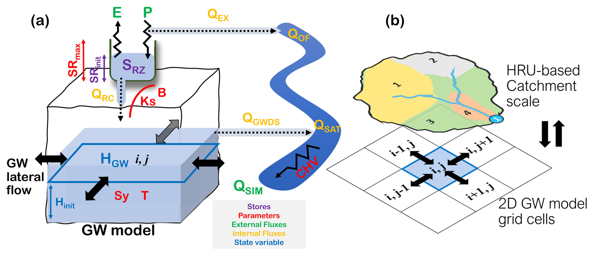
Figure 1Schematic view of (a) the DECIPHeR-GW model structure and (b) the spatial interaction between DECIPHeR HRUs and groundwater model grid cells.
2.2 DECIPHeR-GW model structure
The new coupled DECIPHeR-GW model fully integrates the DECIPHeR and the groundwater models, as shown in Fig. 1, which consists of the HRU-based surface water model component and the 2D-grid-based groundwater model. At each time step, the groundwater model receives recharge values (QRC) from the surface model component, i.e. the root zone storage (SRZ) at the HRU scale; simulates surface–groundwater interactions; and passes the derived groundwater head (HGW) and groundwater discharge (QGWDS) back to the HRUs for the river routing.
The surface water component (e.g. SRZ), as well as the river routing module of the coupled model, was taken from the hydrological model DECIPHeR (Coxon et al., 2019). The root zone store is the main surface water component in the coupled model, which directly interacts with precipitation (P) and evapotranspiration (ET), with a maximum storage determined by the model parameter SRmax. At each time step, precipitation is added to SRZ, and the actual evapotranspiration (ET) is calculated and removed directly from the root zone. Equation (1) was used to derive the actual evapotranspiration (ET) for each HRU, which depends on the potential evapotranspiration rate (PET) and the saturation level of the root zone storage.
SRinit represents the initial root zone storage for each HRU, which requires initialization at the beginning of the simulation. Previous studies (Coxon et al., 2019; Lane et al., 2021) have shown that this parameter exhibits low sensitivity to the model results. Consequently, SRinit was initialized as half of the SRmax in this study instead of behaving as a model parameter for calibration. Once the root zone storage is full, excess rainfall is generated as saturated excess flow (QEX), which is considered to be the saturated overland flow (QOF), and then is added to the river channel for river routing. The coupled model does not consider infiltration capacity.
Recharge QRC from the root zone storage is computed by implementing the nonlinear equation from Famiglietti and Wood (1994), which takes into account the soil hydraulic properties and the storage capacity of the root zone (Eq. 2). In our coupled model setup, recharge is driving the groundwater model component.
where Ks is the saturated hydraulic conductivity (m per time step), and B is the pore size distribution index (dimensionless).
The groundwater model component was developed by Rahman et al. (2023) and uses a transient groundwater flow equation in two spatial dimensions (Eq. 3, Fig. 1b). The finite difference approximation is used to discretize Eq. (3), and an implicit approach is employed to solve it. A no-flow lateral boundary condition is implemented in the model. Spatially, the model domain can be discretized using a user-defined uniform grid according to the topography. With the input of recharge (QRC), groundwater initial head (Hinit), and hydrogeology (i.e. transmissivity T and specific yield Sy) data, gridded groundwater heads (HGW) can be calculated at each time step by solving large sets of linear equations.
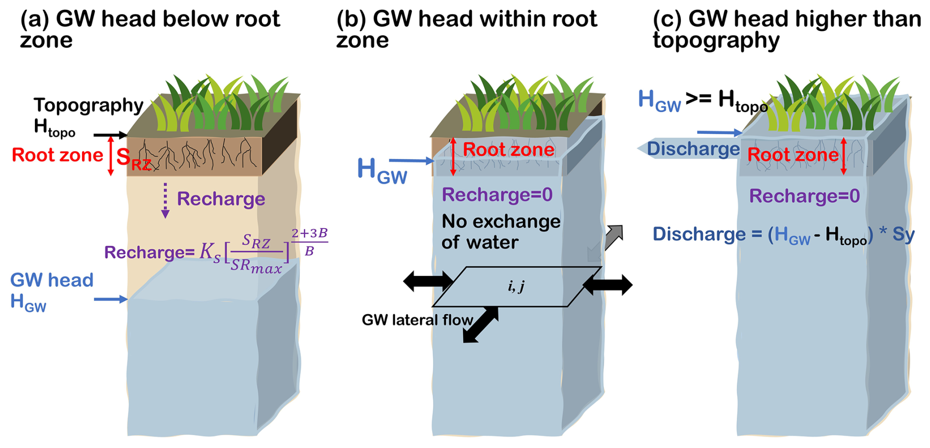
Figure 2Schematic model set-up of surface–groundwater interactions under three scenarios: (a) the groundwater head is below the bottom of the root zone, (b) the groundwater head is within the root zone, and (c) the groundwater head is higher than the topography. The colour coding of the text is as follows: red indicates the root zone, purple represents recharge, and blue denotes the modelled groundwater heads.
Whenever the modelled groundwater head exceeds the topography, groundwater discharge (QGWDS) is calculated using Eq. (4). The groundwater discharge is passed back to the HRUs as saturated flow (QSAT) and added to the nearest river channel for river routing. The surface component from DECIPHeR does not directly account for water flow from the river to HRUs, and the groundwater model lacks explicit river channel representation; thus the coupled model does not capture the river water contribution to aquifer recharge. Instead, aquifer recharge is accounted for via the root zone (see also Fig. 2). Given the high sensitivity of groundwater head simulation to hydrogeological data (Rahman et al., 2023), transmissivity (T) and specific yield (Sy) are selected as model parameters for calibration in the coupled model.
where Sy is specific yield (–), h is the groundwater head (m), t is time, T is transmissivity (m2 per time step), R is the potential recharge rate (m per time step), and htop is the topographic height (m).
Table 1Overview of model stores, fluxes, state variables, and parameters. (mAOD in this table stands for metres above ordnance datum, i.e. sea level).
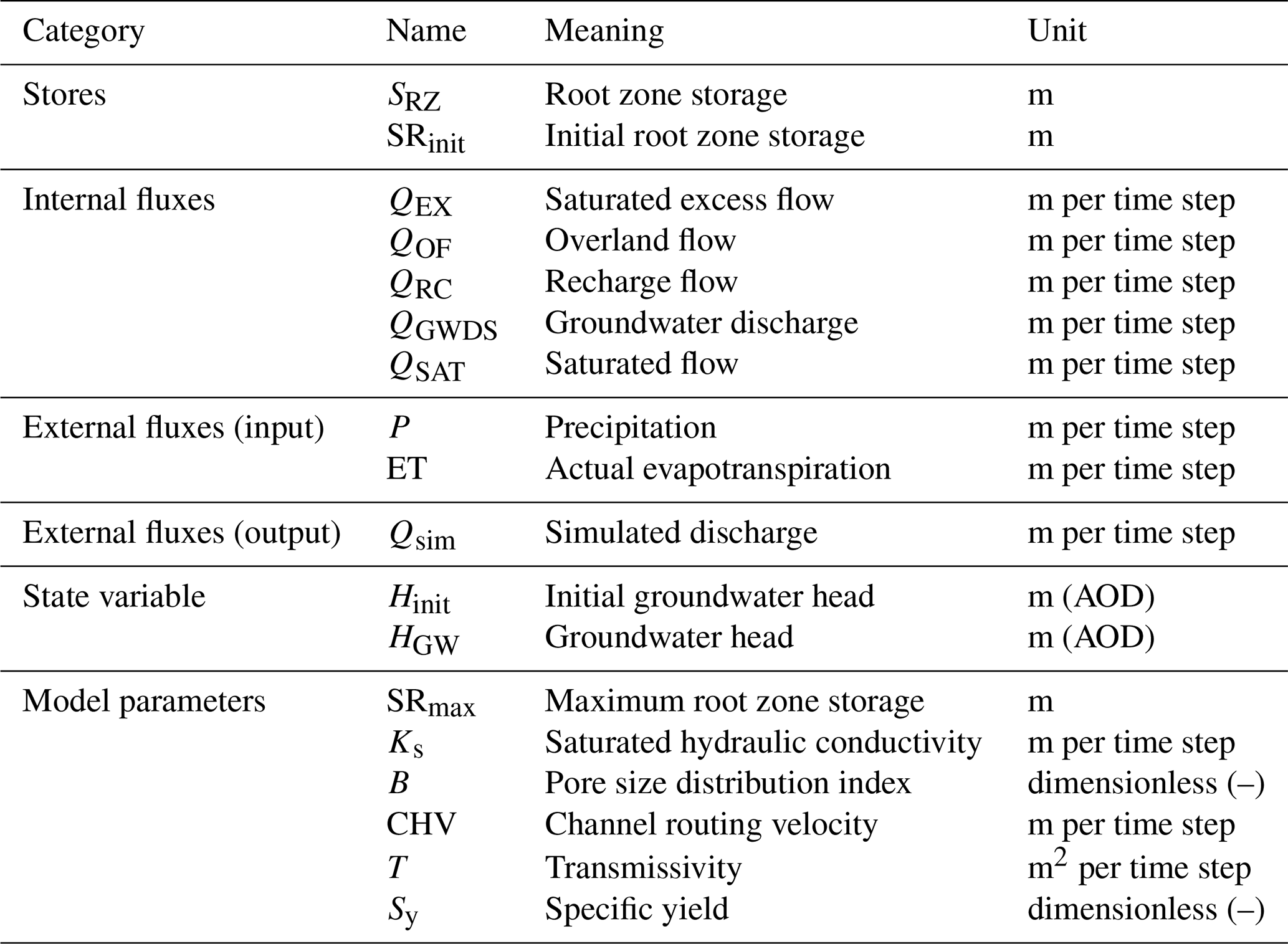
The overview of all model stores, fluxes, state variables, and model parameters is summarized in Table 1. There are six model parameters in the coupled model that can be sampled or set to default values. The model parameters for the surface water and groundwater components are at different scales, and each is prepared independently. The parameters SRmax, Ks, B, and CHV control the surface water model component (including recharge and river routing) at the HRU or catchment scale, which needs soil texture and land use information to determine their parameterization. Parameters T and Sy, which govern the groundwater flow simulation, are determined by a lithology map that matches the spatial resolution of the groundwater grids. Details of the river routing approach can be found in Coxon et al. (2019).
2.3 Surface–groundwater interactions
To represent dynamic surface–groundwater interactions, three scenarios (as shown in Fig. 2a–c) have been implemented in the coupled model setup. At each time step, the position of the groundwater head and root zone storage determines the occurrence and the amount of recharge. For example, if the groundwater head is below the bottom of the root zone (Fig. 2a), we assume that recharge occurs, leaking from the root zone storage to the groundwater system after removing the actual evapotranspiration. As presented in Eq. (2) in Sect. 2.2, the value of the recharge depends on the soil texture and the saturation level of the root zone storage. The recharge was set to not exceed the root zone storage SRZ. The bottom of the root zone is defined as the topography Htopo minus the depth of the root zone DRZ. The root zone depth is estimated using Eq. (5) according to previous studies (Wang-Erlandsson et al., 2016; Lane et al., 2021).
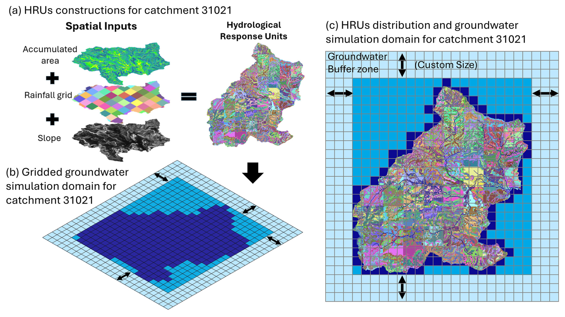
Figure 3The DECIPHeR-GW coupling and spatial interaction from DECIPHeR hydrologic response units (HRUs) to groundwater model grid cells for one example catchment, Welland at Ashley 31021. (a) The HRU construction process for catchment 31021; (b) the gridded groundwater simulation domain for catchment 31021. (c) DECIPHeR-GW coupling and spatial interaction between HRUs and groundwater grids.
If the groundwater head reaches the bottom of the root zone but is below the topography (Fig. 2b), we assume no exchange of water takes place between the surface and groundwater system in this case (i.e. no recharge). In the last scenario, if the groundwater head exceeds the topography (Fig. 2c), groundwater discharge is generated (no recharge). Groundwater discharge is subsequently passed to the HRUs as saturated flow and added to the nearest river channel for river routing.
In all three scenarios, the root zone storage receives rainfall, and actual evapotranspiration is subtracted as usual at every time step (Eq. 1), regardless of the movement of the groundwater heads. Whenever the root zone storage is full, any rainfall excess is generated as overland flow and then added to the river channel.
Given that we build and run the coupled model for each catchment, the groundwater model gridded domain needs to be first determined according to the catchment boundary before the simulations. In our study, we assumed that no water can move and leave the groundwater system across the boundary since a no-flow lateral boundary condition is adopted in the groundwater model. To reduce the effects of this no-flow boundary condition and allow for inter-catchment groundwater exchange, the groundwater simulation domain is extended beyond the catchment boundary in all directions (Fig. 3b). This expanded groundwater gridded simulation area is referred to as the buffer zone in our study (light blue grids in Fig. 3b and c). Absence of the buffer zone could lead to the potential buildup of water in the adjacent cells of the lateral boundaries due to the adoption of the no-flow boundary condition. The groundwater grids and buffer zones outside the catchment boundaries do not incorporate or consider HRUs, which are exclusively confined within the catchment boundaries. Users can customize the size of buffer zone according to the modelling objective. Details on how to determine the appropriate buffer zone size for our analysis are provided in Sect. 3.2. Note that the coupled model is currently designed to run each river basin individually, without accounting for the exchange of hydrological variables such as groundwater flow across river basins. Within each river basin, we do consider the exchange of hydrological variables across catchments. While buffer zones of adjacent river basins may overlap geographically, they remain hydrologically independent and do not interact.
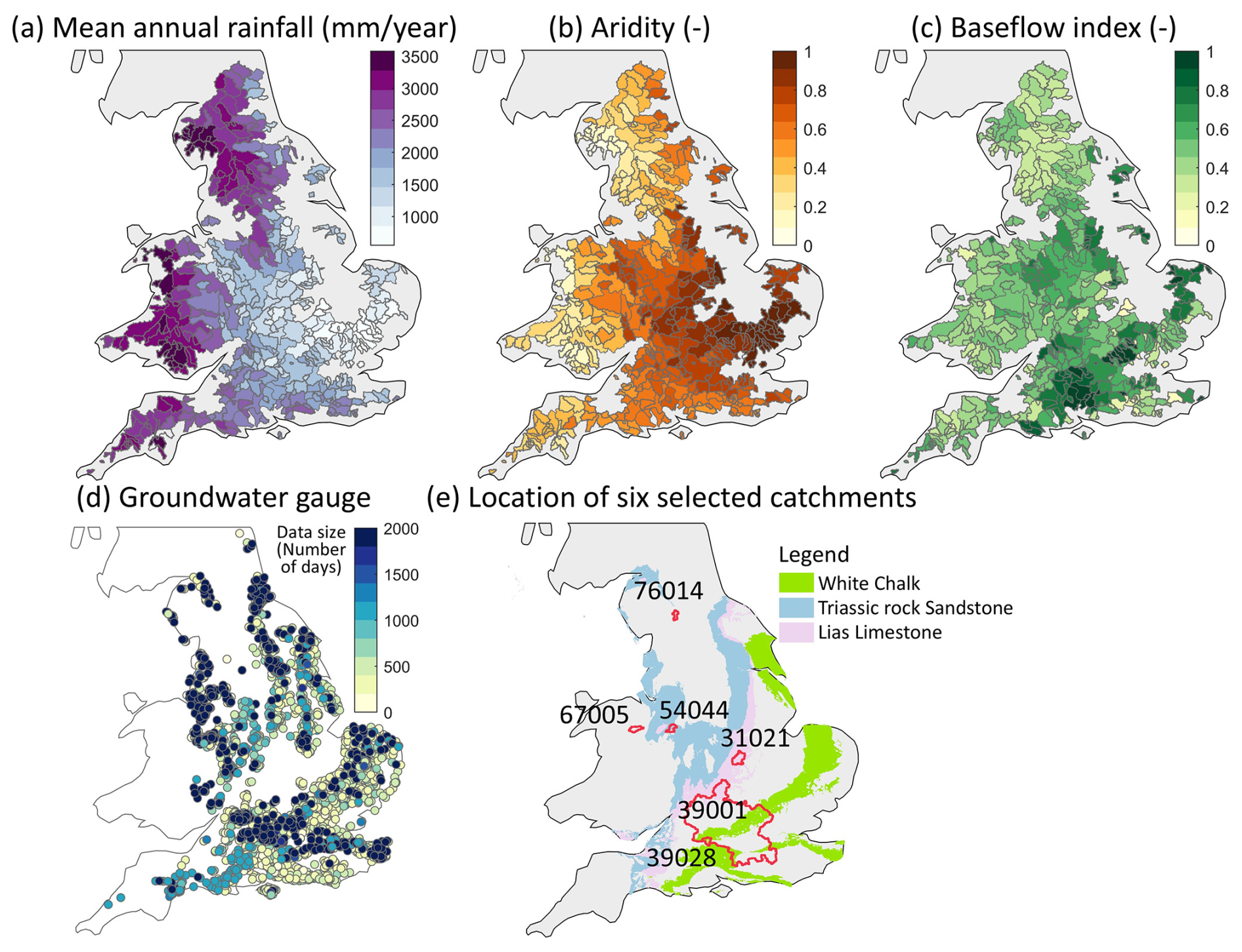
Figure 4Hydro-climate, geology, and available groundwater well locations of the 669 catchments used in this study. (a) Mean annual rainfall (mm yr−1), (b) aridity (–), (c) baseflow index (–), (d) the locations of the 3888 groundwater wells used in this study, and (e) the locations of six selected catchments (details in Sect. 4.2 and Table 4). The map of hydrogeological properties in the background (this figure contains British Geological Survey materials ©UKRI 2020) highlights highly productive aquifers, including white chalk, Triassic sandstone, and Lias limestone.
The recharge, groundwater discharge fluxes, and the state variable groundwater head need to be transferred between surface water component HRUs and gridded groundwater cells. To address this spatial-scale discrepancy between variables, a model mapping scheme is adopted, which follows a similar procedure to coupling the HRU-based SWAT model and gridded groundwater model MODFLOW (Bailey et al., 2016). For a given HRU, the proportion of its area overlapped by different grids is needed to transfer variables from HRUs to grids. Conversely, to transfer variables from grids to HRUs, the proportion of each grid cell area that is occupied by different HRUs is needed. Both these proportions are calculated as the weighting matrix at the beginning of the simulation and stored to transfer variables at each time step. Detailed model mapping methods and the schematic figures can be found in Text S2 and Figs. S1–S3 in the Supplement. Water balance checks were implemented to verify conservation of mass in the coupled model (See Text S3).
3.1 Study area and catchment selection
To test our new coupled model, we apply DECIPHeR-GW over a large sample of catchments across England and Wales. Extensive and high-quality open-source hydro-climate and geological data are available in England and Wales, such as the CAMELS-GB dataset (Coxon et al., 2020), along with a large number of groundwater level observations (Environment Agency, 2023), making it highly suitable for testing and evaluating our coupled model. Also, Great Britain exhibits a wide diversity of hydrogeology features, with geological units spanning a range of ages traceable back to the Pre-Cambrian (Allen et al., 1997), resulting in a wide variety of aquifer types (Fig. S5). This allows us to test the robustness of the coupled model under a range of hydrogeological conditions, modelling for the three principal aquifers: chalk, Permo-Triassic sandstone, and Jurassic limestone (Allen et al., 1997). The chalk aquifer, notably distributed in the southeast of England, is highly permeable, where catchments are connected to a wider regional groundwater system, resulting in inter-catchment subsurface flows (Allen et al., 1997; Oldham et al., 2023). Despite the vast range of hydrological models applied to this region (Coxon et al., 2019; Lane et al., 2019, 2021; Hannaford et al., 2022; Lees et al., 2021; Bell et al., 2007; Ewen et al., 2000; Seibert et al., 2018; Lewis, 2016), deficiencies in model performance persist for these groundwater-flow-dominated catchments. Thus, we test our coupled model over England and Wales, with the aim of improving model performance in these groundwater-dominated regions through a better representation of surface–groundwater interactions.
We selected 669 catchments from all river records in the National River Flow Archive (NRFA) across England and Wales to evaluate the coupled model and represent a variety of hydro-climate characteristics, which ensures the robustness and generalizability of our results. All catchments shown in Fig. 4a–c were selected based on the following data criteria. Note that catchments in Scotland were excluded from our analysis due to lack of access to hydrogeological data.
First, to ensure robust calibration, only catchments with over 20 years of observed data within the calibration period spanning 1980 to 2010 were selected. The model was configured to run from 1970 to 2020 based on data availability, capturing a broad range of climate conditions during this period. The initial 10 years served as a warm-up period, with calibration performed from 1980 to 2010, followed by model evaluation in the subsequent years. Secondly, we excluded catchments that are affected significantly by reservoirs, as the coupled model does not incorporate the reservoir operating rules. Using a suite of hydrological signatures, we identified 25 catchments where reservoirs had a significant impact on the water balance or flow variability and excluded these from our sample (Salwey et al., 2023). Thirdly, catchments with a runoff coefficient (calculated as the ratio of mean annual discharge and mean annual precipitation) greater than 1 were also excluded from the analysis due to potential issues with data quality, missing rainfall data, or substantial human–water interactions that we did not consider in this coupled model.
3.2 Surface water component and groundwater model configuration
For the surface water component, a 50 m gridded digital elevation model (Intermap Technologies, 2009) (also used in Coxon et al., 2019; Lane et al., 2021) was adopted as the basis for the digital terrain analysis to build the river network and define the HRUs across all English and Welsh catchments. Headwater cells were extracted from Ordnance Survey river layers (Ordnance Survey, 2023) and then routed downstream along the steepest slopes in the catchment to create the river network for the coupled model. Defining HRUs is a critical step in the application of the surface water component because these HRUs act as individual model stores with different spatial inputs and model parameter values. In this study, we implemented the same HRU discretization approach described in Salwey et al. (2024), which uses three equal classes of slope, accumulated area, and catchment boundaries, as well as a 2.2 km input grid. This is consistent with the national climate projection data detailed in Sect. 3.3 and higher-resolution input data compared to previous studies using DECIPHeR (Coxon et al., 2019; Lane et al., 2021). The average size of the HRUs generated across all study catchments is 0.31 km2, with HRU areas ranging from the largest, 3.55 km2, to the smallest, which is the size of one DEM grid cell (0.0025 km2).
Table 2Detailed descriptions of the topography, hydro-climate, land use, soil texture, and hydrogeology variables used for model configuration, inputs, parameterization, and evaluation in this study.
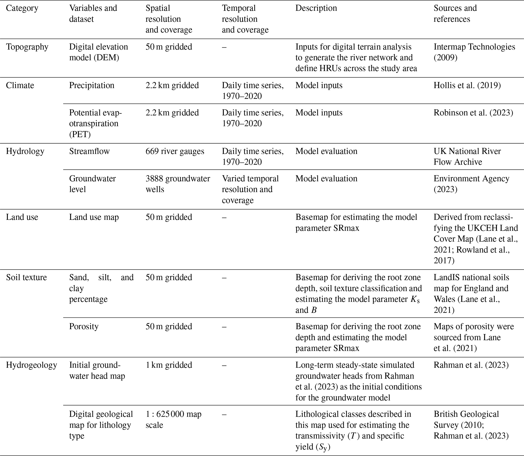
We constructed and operated the gridded groundwater model based on the topography data at a 1 km spatial resolution, which has a comparable scale to the size of HRUs. The groundwater model simulation domain is defined by grids overlaying the catchment boundary and the buffer zone. Text S11 and Fig. S14 in the Supplement provide details of how we determined the buffer zone size, which resulted in a 3 km buffer zone around the catchment boundary to reduce the impact of no-flow boundary conditions. Future users can adjust this buffer value as needed. We used the long-term steady-state simulated groundwater heads from Rahman et al. (2023) as the initial conditions for the groundwater model to ensure that the model achieves a stable and reasonable operational state as quickly as possible. A detailed description of all the topography, hydro-climate, land use, soil texture, and hydrogeology variables that are used for the model configuration, inputs, parameterization, and evaluation is summarized in Table 2. Sections 3.3 and 3.4 introduce more details about the model input and evaluation datasets and model parameterization.
3.3 Input and evaluation datasets
Daily precipitation, potential evapotranspiration (PET), and streamflow and groundwater level data were used to run and evaluate DECIPHeR-GW. For the input data, this study uses the observation-based gridded daily precipitation and PET data derived from HadUK-Grid, a newly produced dataset providing gridded climate observations for the UK at a spatial resolution of 1 km (Hollis et al., 2019). Daily precipitation data from HadUK-Grid, available from 1891 to the present, is derived from the Met Office UK rain gauge network, which is quality controlled, and then inverse-distance-weighted interpolation is applied to generate the daily rainfall grids. Daily PET data, available from 1969 to 2021, is calculated using the Penman–Monteith equation, with climate variables obtained from HadUK-Grid (Robinson et al., 2023). To align with the existing model setup and the grid used for the national climate (Robinson et al., 2021; Lane and Kay, 2022; Salwey et al., 2024), these climate variables were upscaled to a 2.2 km grid for hydrological simulations.
To evaluate the river flows generated in DECIPHeR-GW, daily observed streamflow data sourced from NRFA were used to calibrate and evaluate the model performance. The modelled groundwater levels are evaluated using groundwater level observation data from the Environment Agency's groundwater monitoring network database (Environment Agency, 2023). The groundwater level observations for a total of 3888 groundwater wells in England and Wales were collected, which cover a variety of temporal resolution and coverage with varying levels of data quality. Before using these in model evaluation, several quality control steps were applied to the measured groundwater level data, as illustrated in Fig. S4b. Details of the data quality control are provided in the Supplement (Text S4). There are 3005 wells providing manually measured data (dipped data) at either daily or monthly intervals, while 883 wells offer automatically logged data recorded by pressure transducers at a subdaily scale. Furthermore, there are 395 wells where both types of data are available (see the locations in Figs. 4d and S4a). The temporal coverage varies significantly, with a median of approximately 41 years and the shortest period being just 4 years of noncontinuous observations (Fig. S4c). After the data quality control, data from 1804 groundwater wells were used for the model evaluation.
3.4 Model parameters
A total of six model parameters need to be calibrated to run the coupled model. The SRmax and CHV parameters were already included in the DECIPHeR model structure. For the coupled model, we sampled these two model parameters using the same method following Lane et al. (2021). Specifically, SRmax is sampled by adopting the multiscale parameter regionalization (MPR) strategy, which was first estimated at a high resolution based on the geophysical data and the transfer function and then upscaled to the HRU scale. The channel routing parameter CHV, which is not associated with spatial fields, was not parameterized using MPR and was calibrated through random sampling instead. Details about the sampling method for these two model parameters can be found in the work of Lane et al. (2021).
In addition to the two abovementioned model parameters, we have introduced four new model parameters in the coupled model, i.e. saturated hydraulic conductivity (Ks) and pore size distribution index (B), which interact with the surface water components, and transmissivity (T) and specific yield (Sy), which drive groundwater flow. We use representative ranges of saturated hydraulic conductivity (Ks) and pore size distribution (B) from various soil textures measured from a large sample of soil from Clapp and Hornberger (1978) and Rawls et al. (1982). Maps of soil surface properties (porosity and the percentage of sand, silt, and clay) at a 50 m raster were sourced from Lane et al. (2021) to derive the root zone depth and soil texture classification. Soil texture is classified based on the United States Department of Agriculture (USDA) criteria. Ks and B values were sampled in the corresponding ranges for each soil texture classification using a Monte Carlo method on the high-resolution map (50 m raster) of soil texture, and then the geometric mean was calculated to upscale to the HRU scale for calibration.
Table 3Model parameter range, transfer functions, and catchment attribute data used in this study.
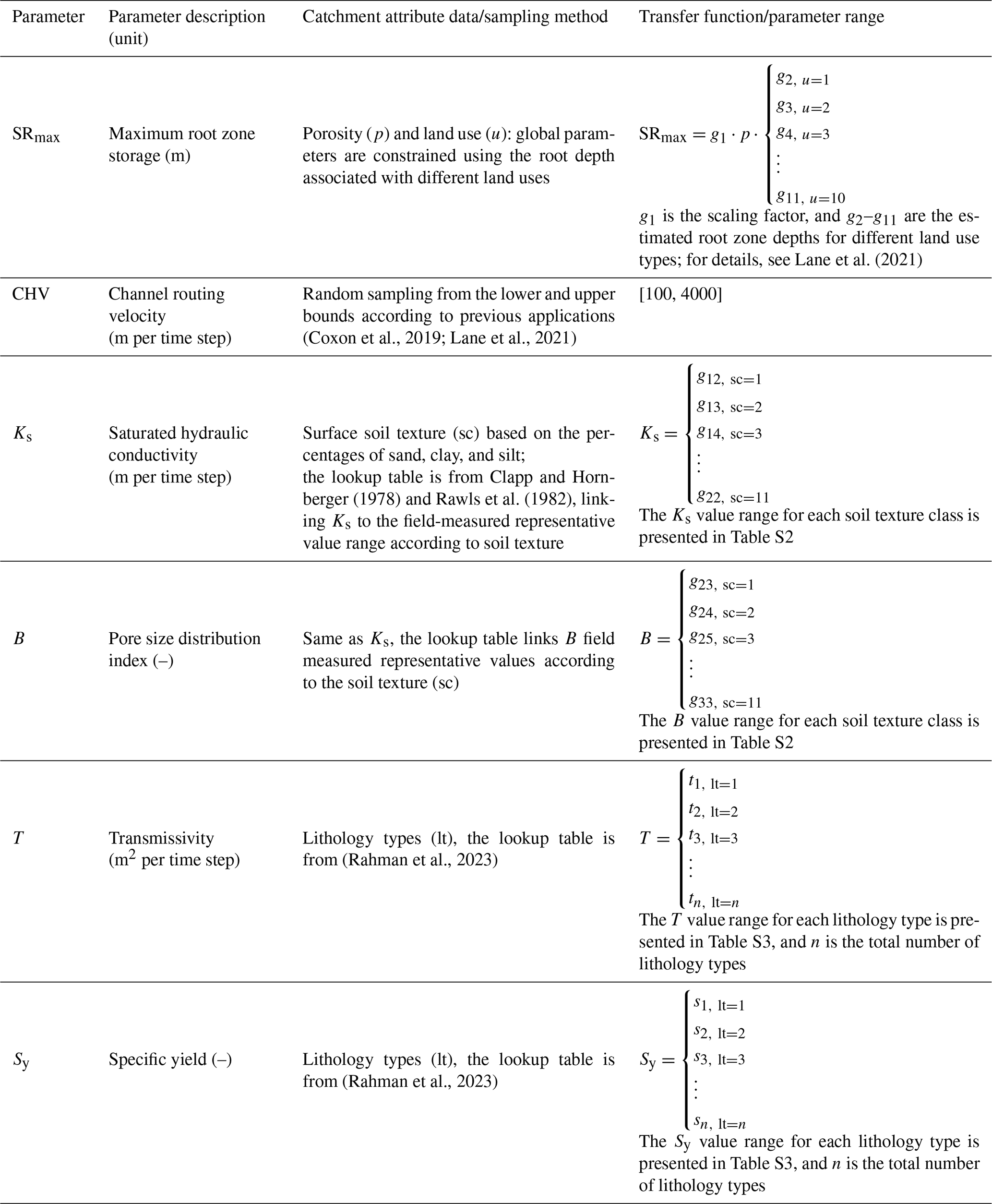
Transmissivity (T) and specific yield (Sy), the parameters of the groundwater component, needed to align with its gridded structure, which is set at a 1 km grid resolution for parameter inputs. Following Rahman et al. (2023), these parameters can be obtained from the representative ranges for different lithology classes based on an extensive literature review and reports for England and Wales (Allen et al., 1997; Jones et al., 2000). The 1:625 000-scale digital geological map of the United Kingdom developed by the British Geological Survey (BGS) is used to provide the lithology classes at 1 km grid resolution. By adopting this lithology map and the lookup table from Rahman et al. (2023), the parameter values of T and Sy can be sampled using the Monte Carlo method for every 1 km grid cell. Table 3 summarizes the functions, parameter ranges, and catchment attribute data used in this study to sample the model parameters. The lookup tables for linking Ks and B with soil texture classes and T and Sy with lithology types, as well as the detailed parameter ranges, are provided in Tables S2 and S3. Since the model parameters are linked with the soil and lithology types, catchments with the same spatial attributes will be calibrated with the same set of model parameters.
3.5 Model calibration and evaluation
In this study, we set up the simulations for 669 catchments, using the DECIPHeR model introduced by Lane et al. (2021) as the benchmark model for comparison with the DECIPHeR-GW model. The DECIPHeR model in Lane et al. (2021) employs the multiscale parameter regionalization (MPR) method to parameterize model parameters while maintaining the original DECIPHeR model structure (Coxon et al., 2019) without groundwater representation. The objective is to utilize these simulations as a benchmark to evaluate the performance of the coupled model after implementing the groundwater process representation. Note that these benchmark model runs are calibrated and evaluated using the same method as the coupled model described below.
We use nonparametric Kling–Gupta efficiency KGE metrics (Pool et al., 2018) to calibrate and evaluate the model results, which comprise three components accounting for the errors in mean flow, flow variability, and the correlation between observed and simulated flow. This nonparametric KGE is proposed to avoid overfitting to particular hydrograph elements. In contrast to the parametric KGE (Gupta et al., 2009), this metric incorporates the difference between flow duration curves (FDCs) to indicate variability instead of standard deviation and employs the Spearman correlation in place of the Pearson correlation coefficient.
Both the coupled and benchmark models were calibrated and evaluated across all 669 catchments by running 5000 simulations in each catchment (i.e. each of the 5000 regionalizations of parameters g1–g33, t1–tn, and s1–sn mentioned in Table 3 is used for all catchments). The model simulates the period from 1970 to 2020 at a daily time step. Simulations from 1970 to 1979 were treated as a warm-up period, and the nonparametric KGE was calculated separately for the calibration period from 1980 to 2010 and the evaluation period spanning 2011 to 2020. These periods were selected as a suitable test for the model, encompassing a variety of climatic conditions to showcase its ability to reproduce major national-scale hydrological extremes, including floods in 2007, 2015, and 2019, as well as droughts in 1984, 2003, 2011, and 2018. Two calibration approaches, namely (a) catchment by catchment and (b) nationally consistent calibration, were used to calibrate the coupled model following the study of Lane et al. (2021). These two calibration methods are applied separately to identify the corresponding best-performing parameters, with the parameter values saved for their respective applications. The first calibration, the catchment-by-catchment calibration, is to find the best-performing simulation (maximum KGE across 5000 simulations) and its corresponding parameter sets for each catchment. The second calibration, the nationally consistent calibration scheme, enables us to identify the best national model parameter sets across all catchments. The median KGE across all catchments is calculated for each simulation, and the nationally consistent approach selects the simulation with the highest median KGE. The second calibration approach is beneficial for national model parameter regionalization, offering valuable insights into model parameter selection for model application in ungauged catchments. In contrast, the first calibration method demonstrates the optimal performance achievable by our coupled model. For the nationally consistent calibration approach following Lane et al. (2021), catchments with maximum KGE values below 0.3 in the first calibration method (catchment by catchment) were excluded from the median KGE calculation. This exclusion avoids catchments where the model structure was not suitable, while retaining as many catchments as possible.
Furthermore, modelled groundwater levels are assessed using a large sample of groundwater level observations from 1804 wells in England and Wales (described in Sect. 3.3) for the model evaluation. Due to the scale discrepancy between the 1 km grid-scale-simulated groundwater level and point-scale observations of specific wells, we use the Spearman correlation coefficient to quantify the ability of the coupled model to reproduce the temporal correlation and do not calculate the bias.
4.1 Overall model performance across catchments
Figure 5a presents the nonparametric KGE values of the simulated streamflow for the coupled model across 669 streamflow gauges during the evaluation period. The calibration results, which are consistent with evaluation results, are detailed in the Supplement (Fig. S6). Using the catchment-by-catchment calibration method (Fig. 5a–d), overall, the coupled model performs well in simulating streamflow across catchments, with a median KGE of 0.83 and most catchments (81 %) achieving 0.7 or higher. Figure 5b illustrates the KGE differences between the coupled model and benchmark runs using DECIPHeR. Approximately 70 % of the catchments exhibit KGE differences of 0.1 or less between the coupled and benchmark models, indicating that the coupled model achieves comparable results with those of the benchmark model.
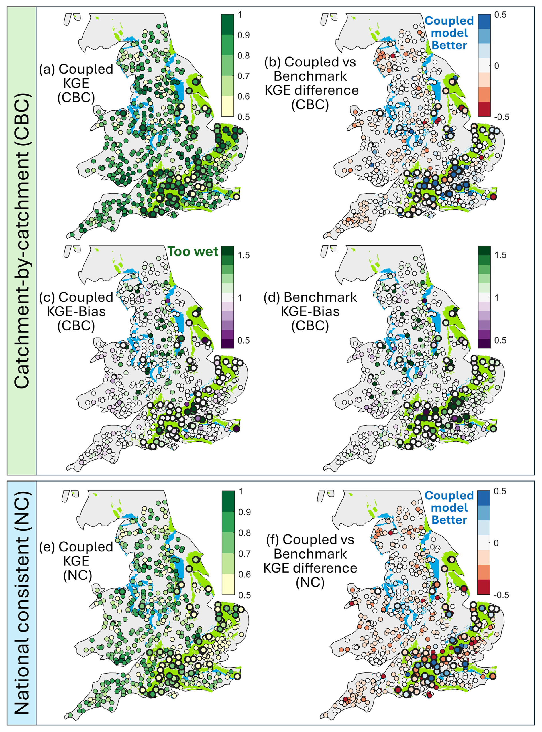
Figure 5Spatial maps of model performance using two calibration approaches: (a) the catchment-by-catchment (CBC) and (b) the nationally consistent (NC) approaches. The nonparametric KGE differences between the coupled model and the corresponding DECIPHeR benchmark runs (b, f), and the bias component of KGE for the coupled model and benchmark runs for the CBC approach (c, d) are also included. The maps for other KGE components are provided in the Supplement (Fig. S7). Each dot represents the performance at a river gauge during the evaluation period. Model performance maps for the calibration period are provided in the Supplement (Fig. S6). The scattered dots for groundwater-dominated catchments (baseflow index > 0.75) were labelled with larger dots and outlined with thicker borders. The background of the maps highlights the areas of high productivity in aquifers (this figure contains British Geological Survey materials ©UKRI 2020). Light green represents highly productive aquifers (fracture flow), while blue indicates the intergranular flow of a highly productive aquifer.
Notably, the coupled model demonstrates better performance in groundwater-dominated chalk catchments with a baseflow index > 0.75 (blue dots in Fig. 5b), where the average KGE improves from 0.49 with the benchmark model to 0.70. In the southeast's chalk region, the coupled model achieves KGE improvements exceeding 0.35 in 20 catchments, with 6 catchments showing improvements greater than 1. In contrast, the benchmark model performs slightly better in the western regions of England and Wales (indicated by orange dots in Fig. 5b), where catchments are wetter, with mean annual rainfall exceeding 1500 mm yr−1, achieving a median KGE around 0.88. Nevertheless, the coupled model still maintains a median KGE of 0.80 for these wetter catchments. The comparison of the KGE bias component between two models, as displayed in Fig. 5c and d, further confirms that the coupled model improves the reproduction of the water balance for these groundwater-dominated catchments in the southeast, particularly those in the Thames River basin. However, the coupled model still tends to overestimate streamflow in some catchments in central and southeast England, which could be due to human activities such as surface water and groundwater abstractions (Salwey et al., 2023; Wendt et al., 2021b; Bloomfield et al., 2021).
As expected, a performance drop is observed in the nationally consistent calibration strategy (Fig. 5e and f) since the parameterization is not optimized for individual catchments. Compared to the catchment-by-catchment calibration, approximately 50 % of catchments experienced a decline of less than 0.1 in KGE for the coupled model, whereas 64 % experienced a decline for the benchmark. The decrease in KGE scores is primarily concentrated in the southeast of England, echoing the findings of Lane et al. (2021). This might be attributed to the method used for catchment selection in the national regionalization process. Groundwater-dominated catchments with a baseflow index > 0.75 account for less than 10 % of the total catchments calibrated in this study. By assigning equal weights to all catchments, the model parameters for groundwater-dominated catchments might not be constrained properly under the nationally consistent approach, leading to reduced performance in those areas. However, despite the reduced performance using the nationally consistent calibration method, the coupled model still outperforms in approximately 50 % groundwater-dominated catchments compared to the benchmark model (Fig. 5f). Future work is suggested to explore alternative weighting approaches to enhance parameter calibration, instead of using equal weighting.
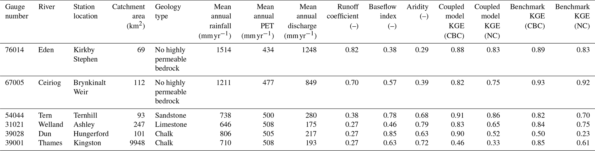
Table 4Catchment attributes and model performance for the six selected catchments. Their locations are presented in Fig. 4e; simulated hydrographs are shown in Fig. 6. Baseflow index and aridity are derived from the CAMELS-GB dataset (Coxon et al., 2020). The runoff coefficient is calculated as the mean annual discharge divided by the mean annual rainfall. The KGE values presented in this table were calculated for calibration periods using catchment-by-catchment (CBC) and nationally consistent (NC) calibration approaches. Benchmark KGE represents the results from DECIPHeR.
4.2 Performance of simulated flow time series
Six catchments were selected to demonstrate the coupled model's ability to reproduce the streamflow time series with distinct characteristics, i.e. climate conditions, geology types, and levels of human impact (Table 4). Specifically, catchments 76014 and 67005 were selected to evaluate coupled model performance in a wet climate (mean annual rainfall > 1200 mm yr−1), while 39028 and 39001, differing in human impact, represented dry chalk catchments. Catchment 31021 was chosen for limestone and 54044 for sandstone. The simulation of the 2-year period from 2010 to 2012 using the calibration period model parameters is presented here for these catchments, as it encompasses diverse hydrological extreme events (Marsh et al., 2013). The evaluation period model parameters exhibit a similar pattern and will not change the analysis herein.
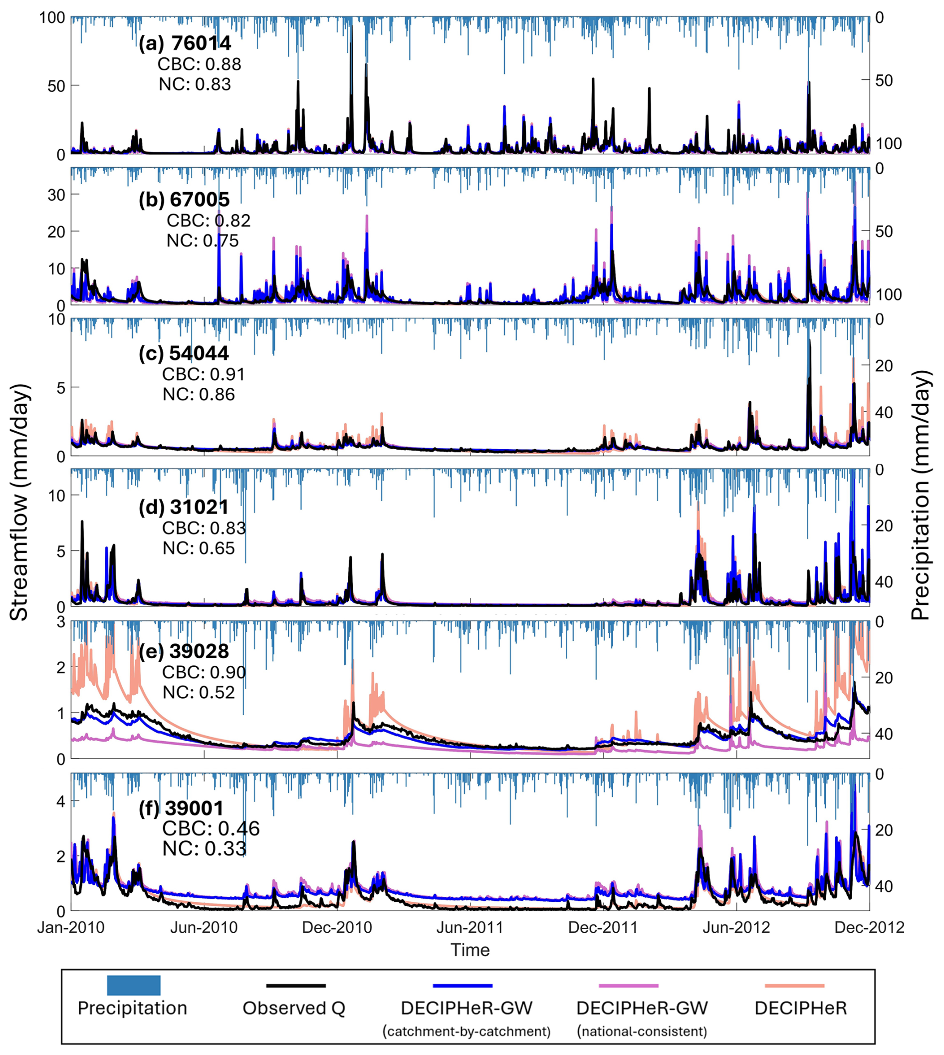
Figure 6The observed and the best simulated streamflow hydrographs using the model parameters from the calibration period for the six catchments across different catchment attributes (shown in Table 4). The best simulated DECIPHeR-GW hydrographs along with their KGE values for both the catchment-by-catchment (CBC) and nationally consistent (NC) approaches are provided. The DECIPHeR model simulation results (the orange line) presented here are based on the CBC calibration method. To enhance clarity and simplify the visuals, the simulation results for the NC calibration method from DECIPHeR are not plotted here, but the KGE metrics for each catchment using the NC calibration method are detailed in Table 4.
Figure 6 illustrates DECIPHeR-GW results for a wide spectrum of hydrological dynamics, including the wetter catchments in northwest England and north Wales (Fig. 6a and b), as well as the drier catchments in the southeast (Fig. 6e and f). Especially in the groundwater-dominated chalk catchment (39028) that is characterized by small net loss from abstractions and discharge (minor human influences) and is essentially a natural baseflow-dominated flow regime, the streamflow hydrograph simulations from the coupled model significantly improve and fit well compared to observations (Fig. 6e), with the KGE metric increasing almost 2-fold compared to the benchmark when using both the catchment-by-catchment and the nationally consistent calibration methods (showed in Table 4). In addition, when using the catchment-by-catchment calibration method, the coupled model performed well for other aquifer types, as shown by the results from limestone catchment 31021 (Fig. 6d) and sandstone catchment 54044 (Fig. 6c), with KGE values exceeding 0.80. The simulated streamflow hydrograph using the nationally consistent calibration method also closely aligns with the results from the catchment-by-catchment calibration method, with relatively larger differences in performance observed in groundwater-dominated catchments (Fig. 6e).
In the Thames at the Kingston River basin (catchment ID 39001), where surface water and groundwater abstractions are prevalent, the coupled model tends to overestimate flows during the dry periods in particular (Fig. 6f). Wastewater returns from sewage treatment are also common in these regions and could influence streamflow (Coxon et al., 2024), potentially contributing to the decline in KGE performance. This decline in performance indicates the challenge of simulating flows in heavily human-impacted catchments and underscores the need to enhance the representation of human–water interactions in the hydrological model. Meanwhile, it is interesting to see that the benchmark model produces better simulation results for a catchment with significant human activities, such as the Thames River basin, with a KGE of 0.85 using the catchment-by-catchment calibration method despite not accounting for either groundwater or human–water interactions. This implies that the benchmark calibration could produce good results, potentially due to the parameterization that compensates for the absence of these process representations. Ensuring that the model performs well with appropriately structured components is crucial to maintain both accuracy and reliability (Kirchner, 2006; Gupta et al., 2012).
Furthermore, the simulated streamflow hydrographs for the wetter catchments tends to be flashier than the benchmark simulations (as shown in catchment 67005, Fig. 6b). This might be related to the relatively wet conditions of the catchment in combination with the underlaying groundwater system being already saturated or nearly saturated. Once the root zone reaches capacity, runoff is quickly generated as excess rainfall, leading to a rapid response to precipitation and resulting in more pronounced spikes in the hydrographs. The dynamic variations in these internal variables for this catchment during 2010–2012 are provided in the Supplement (Fig. S8). However, for most wet catchments (mean annual rainfall > 1500 mm yr−1 ), the coupled model performs well (examples in catchment 76014, Fig. 6a), with around 78 % of these catchments achieving a KGE greater than 0.7.
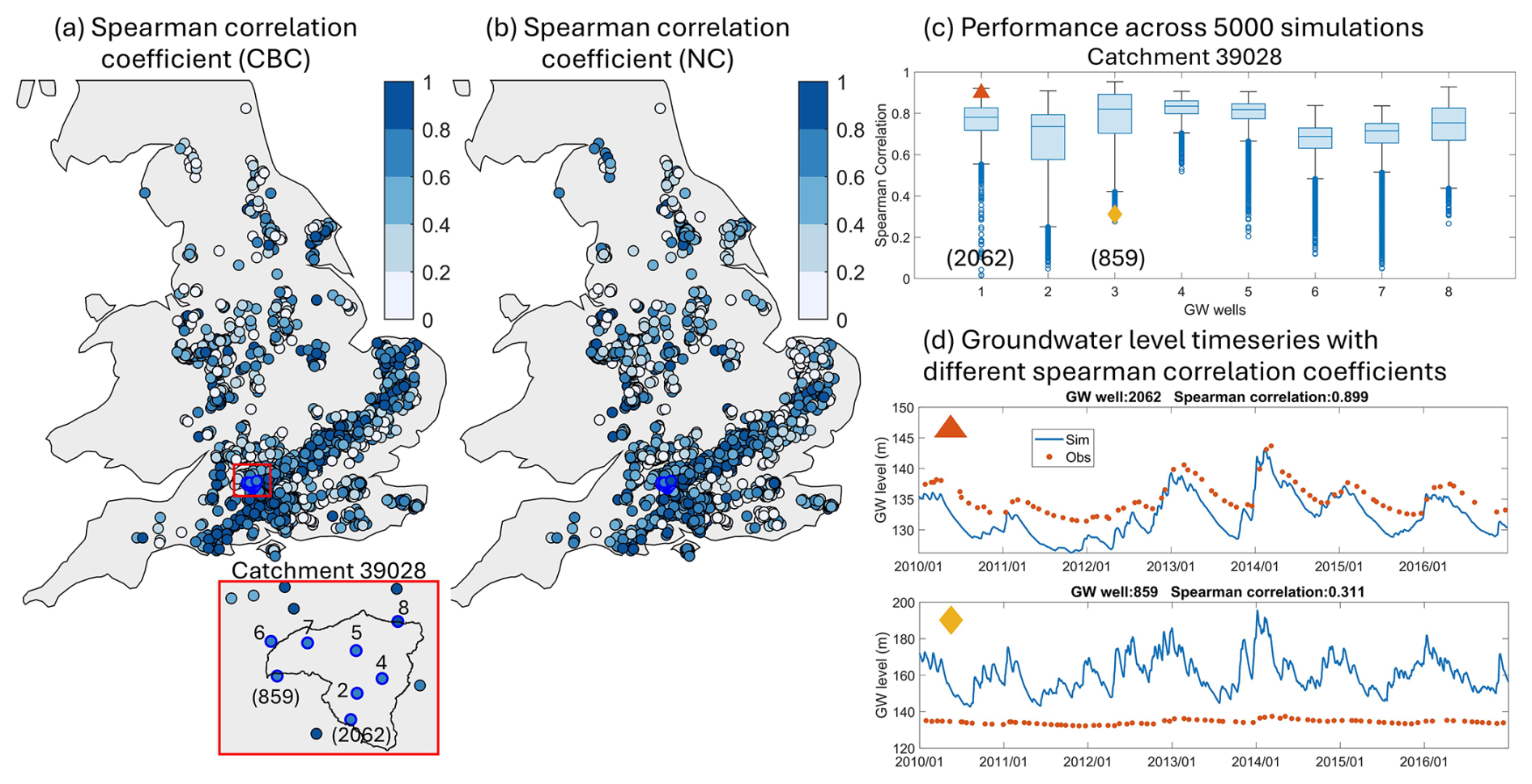
Figure 7Spatial maps of groundwater level evaluation results. Panels (a) and (b) show the evaluation results for the simulated groundwater levels using the catchment-by-catchment (CBC) and nationally consistent (NC) streamflow calibration methods, respectively. Panel (c) presents the performance of the eight groundwater grids in the Dun at Hungerford catchment (39028) across 5000 simulations using the catchment-by-catchment calibration method. Panel (d) displays the simulated groundwater level time series compared with the observations from two wells, demonstrating cases with strong and weak Spearman correlation coefficients. The example groundwater time series is shown for two wells at Old School House (GW well 2062) and East Wick Farm (GW well 859).
A simple model parameter sensitivity analysis (details provided in Supplement Text S10) reveals that the parameters of the surface model component have a greater influence on simulated streamflow hydrographs than on modelled groundwater levels (as seen in Figs. S10 and S13). SRmax, which determines the maximum root zone storage, plays a crucial role in regulating the flashiness of simulated flows (Fig. S10a). Smaller SRmax values lead to increased variability in runoff, as runoff is rapidly generated whenever SRmax reaches its capacity, causing spikes in the hydrographs due to excess rainfall. Both the B and Ks parameters control the magnitude of recharge, as shown in Fig. S10b and c; their effects on simulating streamflow hydrographs are similar, with a relatively greater impact observed for the B parameter. Smaller B values lead to reduced recharge, causing the root zone storage to fill up more quickly and resulting in increased overflow and also flashier in-streamflow hydrographs. The groundwater-related parameters, i.e. T and Sy, are intended to control groundwater levels more than streamflow, which is confirmed by this analysis (see Figs. S11 and S12). Consequently, this sensitivity analysis indicates that increasing SRmax or B values could result in smoother streamflow hydrographs and therefore might improve DECIPHeR-GW's performance in wetter catchments.
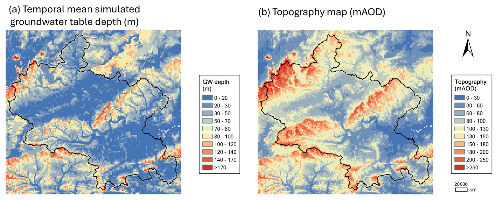
Figure 8Spatial maps of simulated groundwater table depth for Thames at Kingston 39001. (a) Temporal mean over 1980–2020 of simulated groundwater table depth (difference between the local topography and the groundwater head in metres below land surface) in catchment 39001 using the best catchment-by-catchment calibration method. (b) The topography map for catchment 39001.
4.3 Model evaluations with groundwater levels
We used 1804 groundwater well observations to evaluate grid-scale simulated groundwater levels. In this study, we calibrated the model solely using streamflow data as our objective, while utilizing groundwater observations to evaluate the internal dynamics of the coupled model. Figure 7a and b illustrate groundwater simulations corresponding to the best streamflow simulations using two streamflow calibration methods, i.e. catchment by catchment and nationally consistent. Overall, the groundwater simulation results are generally able to capture the temporal correlation of the observations, particularly in the chalk region, where over 75 % of wells achieve Spearman correlation coefficients above 0.6, with a median of 0.77. The results are highly consistent between the two streamflow calibration methods (Fig. 7a and b), indicating that the coupled model is robust in simulating the groundwater levels. The spatial distribution of the temporal mean simulated groundwater table depth over 1980–2020 for the Thames at Kingston catchment 39001, a groundwater-dominated catchment and one of the largest in our study area, is presented in Fig. 8, which is based on the best catchment-by-catchment calibration method. The simulated groundwater table depth aligns consistently with topographic trends, confirming that our coupled model also accurately reproduces the spatial variability in the groundwater table.
Taking catchment 39028 as an example, Fig. 7c demonstrates that model performance can vary across 5000 simulations using the catchment-by-catchment calibration method. The median Spearman correlation coefficients for different groundwater grids across all simulations in general reach 0.6 or higher. A portion of the groundwater wells has a median Spearman coefficient for groundwater levels exceeding 0.8 (see groundwater wells 3, 4, and 5 in Fig. 7c), underscoring the model's ability to reproduce the temporal patterns of groundwater variations. Figure 7d presents two examples of simulated groundwater level time series against well observations. While these examples are not from the best simulations, they are chosen to demonstrate the model's performance under conditions of both strong and weak temporal correlation.
Figure S12 illustrates the impact of T and Sy model parameters on the groundwater level time series for example catchment 39028 (details are recorded in Text S10). Higher T values generally result in lower groundwater levels, which is to be expected, as higher transmissivity (T) facilitates quicker lateral flow through an aquifer. In contrast, when Sy is low, the speed of groundwater flow and storage capacity may be reduced, resulting in flashier groundwater levels increasing their variability. Our results confirm the above patterns, showing that higher T leads to decreased groundwater levels and lower Sy leads to greater variability (Fig. S12a and b), highlighting the overall agreement and good representation of physical processes of our coupled model.
Given the poorer temporal correlation observed in some wells, we investigated the factors that could contribute: short groundwater observation records; low streamflow accuracy in catchments; the distance between wells and rivers; and attributes like borehole depth, elevation of wells, and grid elevation contributed to the discrepancies. Our findings point towards key factors, such as borehole depth, river proximity, and streamflow accuracy, which might be affecting the model's ability to model groundwater levels accurately (see details in Fig. S9). We have found lower Spearman correlations for wells with deeper boreholes, for those closer to the river, or for the wells with lower streamflow simulation accuracy. This is likely because our groundwater model is 2D without explicit river feature representation, which can result in lower performance for wells that are deeper or closer to rivers. More details are discussed in Sect. 5.2.
5.1 Enhanced performance of DECIPHeR-GW in groundwater-dominant catchments
Based on the evaluation of 669 river flow gauges and 1804 groundwater monitoring sites across England and Wales, our coupled model DECIPHeR-GW v1.0 is able to produce robust streamflow simulations whilst capturing temporal dynamics of groundwater levels. Notably, the model achieves better performance when simulating river flows in groundwater-dominated catchments, with a baseflow index > 0.75 (Fig. 5b), especially when simulating of catchments with minor human influence, showing significantly higher performance compared to the DECIPHeR model. This improvement is most evident in the chalk regions with strong surface–groundwater interactions, where it reproduces the observed hydrographs (examples in Fig. 6e) and enhances hydrological simulation reliability. Moreover, the coupled model also performed well in other aquifer types including sandstone and limestone (Fig. 6c and d). Although our coupled model exhibits similar or slightly better performance compared to the benchmark model in around 70 % of the catchments, the coupled model has a more robust and reliable structure due to the better representation of the groundwater processes. Herein, the coupled model was able to avoid the unrealistic model parameterizations to compensate for the absence of groundwater representations (Kirchner, 2006; Coxon et al., 2014; Dang et al., 2020). Furthermore, our groundwater component provides groundwater simulation results that compare well to observations with high computational efficiency. Some relatively simplified models only produce groundwater storage (Yang et al., 2017; Guimberteau et al., 2014; Griffiths et al., 2023; Müller Schmied et al., 2014), while some models have adopted a lumped groundwater model structure, failing to capture spatial variability in groundwater distribution (Yeh and Eltahir, 2005; Gascoin et al., 2009; Ejaz et al., 2022). Our model provides simulated groundwater level at the grid scale, facilitating model validation against groundwater observations and producing the spatial groundwater distribution. Although our 2D groundwater model ignores vertical water movement, it is structurally simpler compared to more complex 3D models (Bailey et al., 2016; Ewen et al., 2000; Maxwell et al., 2015; Naz et al., 2022), making it better suited for large-scale simulations and allowing for multiple model calibrations. Hence, the well-matched results for streamflow, parameter sensitivity, and groundwater level patterns show the potential of DECIPHeR-GW for future applications, especially under climate change.
Additionally, the DECIPHeR-GW v1.0 model is a promising tool for water resource management in southeast England, as existing hydrological models in the UK have faced challenges in accurately simulating streamflow and groundwater heads in these groundwater-dominated catchments. For instance, Lane et al. (2019) assessed four different conceptual hydrological models (TOPMODEL, ARNO/VIC, PRMS, SACRAMENTO) through the framework for understanding structural errors (FUSE) across over 1000 catchments in England, Wales, and Scotland. Their findings revealed that these models struggled to simulate biases, standard deviations, and correlations, particularly for the groundwater-dominated catchments in southeastern England. Similar issues have been reported with other models, including a grid-to-grid (G2G) simulation over 61 catchments in Great Britain (Rudd et al., 2017), the GR4J application across 303 UK catchments (Smith et al., 2019), the SHETRAN performance in 306 UK catchments (Seibert et al., 2018; Lewis, 2016), and the SWAT simulation in 2 medium-scale catchments within the Thames River basin (Badjana et al., 2023). Efforts have been made to improve the groundwater representation in hydrological models like GR6J and PDM (Pushpalatha et al., 2011; Moore, 2007). However, models are still unable to accurately capture low flows in some groundwater-influenced catchments, such as those in the eastern Chilterns north of London (Hannaford et al., 2023). Even machine learning models like long short-term memory (LSTM), while generally outperforming conceptual models, struggle to accurately simulate streamflow in the groundwater-dominated catchments (Lees et al., 2021). Moreover, most of these models mentioned above cannot simulate the time series of groundwater heads at the same time as they produce streamflow time series. In this study, our coupled model enables the simulation of inter-catchment subsurface flow and captures the dynamic surface–groundwater interactions well, providing a more precise representation of runoff and groundwater generation process in groundwater-dominated catchments. Consequently, the DECIPHeR-GW model shows potential for future applications, such as in low-flow simulation and drought prediction, particularly in groundwater-dominated catchments.
Furthermore, our coupled model is relatively efficient in terms of computational requirements. One simulation over 51 years for the largest catchment, the Thames at the Kingston River basin (9948 km2), with 27 980 HRUs, takes approximately 17 h to run on a standard CPU, producing simulated streamflow and groundwater level time series for all 98 upstream river gauges and 416 groundwater grids simultaneously. A 51-year simulation of the smallest river basin (10 km2), with 52 HRUs and 1 river gauge, completes in about 1 s using a CPU. Future enhancements in computational efficiency of the coupled model can be achieved by employing sophisticated parallel computing techniques. Our groundwater component omits vertical water flow and river representation, requiring only two subsurface hydrogeological properties. Our model may encounter challenges in regions with significant vertical hydrogeological variability, requiring additional tests in future work for these regions to ensure accuracy. In contrast, some complex 3D groundwater models need to discretize aquifers vertically and include specialized modules for river simulation (Bailey et al., 2016; Ewen et al., 2000; Ng et al., 2018; Maxwell et al., 2015), demanding finer-resolution hydrogeological data to capture land surface heterogeneity and higher computational costs. Currently, lots of existing coupled surface–groundwater models either cannot perform or require excessive time for calibration due to high computational costs (Ng et al., 2018; Parkin et al., 2007; Naz et al., 2022; Reinecke et al., 2019), which limits their ability to assess uncertainty in the presented results and hinders future model applications. The computationally efficient feature of our proposed model allowed us to calibrate it against extensive observed data, including 669 streamflow gauges and 1804 groundwater wells, thereby providing reliable results for future application.
5.2 Lessons learned from model coupling and ongoing developments
As awareness of the importance of groundwater process-based representation grows, along with the rapid development of groundwater models with a variety of complexities, there is a growing interest in incorporating groundwater representations into hydrological or land surface models (Gleeson et al., 2021; De Graaf et al., 2017; Maxwell et al., 2015; Irvine et al., 2024; Ntona et al., 2022). When designing coupled models, balancing model complexity with computational efficiency is crucial (Condon et al., 2021; Barthel and Banzhaf, 2016; Henriksen et al., 2003). Therefore, we selected a computationally efficient 2D model (Rahman et al., 2023), which generally yields superior results. However, this model lacks the representation of the river network and assumes that groundwater above topography is directly discharged into the nearest river, leading to inaccuracies in capturing groundwater dynamics in some low-elevation areas where simulated groundwater levels stay at the surface (see the example in Fig. S15). In addition, to achieve a simpler and more efficient structure of the coupled model, we removed the unsaturated zone from the benchmark DECIPHeR model and directly replaced the saturated zone with the groundwater model. This approach is consistent with many existing coupled models that do not account for the unsaturated zone and generally provide robust simulations (Yang et al., 2017; Jing et al., 2018; Reinecke et al., 2019; Müller Schmied et al., 2014; Henriksen et al., 2003). According to our results, while this approach worked well in most catchments, the absence of an unsaturated zone led to flashier hydrographs in some wetter catchments, where the unsaturated zone is critical for the storage of excess rainfall (Dietrich et al., 2019; Hilberts et al., 2007). Thus, future researchers are advised to explore and design model structures tailored to their specific needs.
Parameterizing surface–groundwater coupled models across large scales and diverse geological types remains challenging due to the difficulty of accurately representing geological heterogeneity (Gleeson et al., 2021; Condon et al., 2021). In our study, groundwater level simulations are highly dependent on hydrogeological parameters (i.e. T and Sy; see sensitivity analysis in Fig. S12). Although we have attempted to capture the complexity of geological conditions using different parameter ranges across 5000 simulations for a total of 101 lithology types, parameters for the same lithology type can only be assigned the same set of values for one simulation. In reality, parameters such as T can vary significantly even within the chalk aquifer (Allen et al., 1997). A recent study presented a 3D geological digital representation model of Great Britain using extensive geological maps and borehole data (Bianchi et al., 2024). They developed a national-scale groundwater model of Great Britain (BGWM) using this detailed geological data to consider the heterogeneity characteristics of aquifers, demonstrating the model's ability to accurately simulate groundwater dynamics. Griffiths et al. (2023) developed a method to estimate the initialized groundwater model parameter set using national-scale hydrogeological datasets to improve the parameterization of New Zealand's national groundwater model. Adopting more accurate and detailed geological data and advanced sampling methods to parametrize the model could be another direction for the further improvement of the model performance (Hellwig et al., 2020; Henriksen et al., 2003; Westerhoff et al., 2018).
Since our coupled model retains the digital terrain analysis (DTA) configuration of the DECIPHeR model (Coxon et al., 2019; Lane et al., 2021) and currently operates at the river basin scale, each river basin is configured and run individually rather than modelling the entire continent or nation. There is no consideration of hydrological variable exchanges, such as groundwater flow, across river basins. Additionally, this setup can result in inaccuracies for small, isolated catchments, as groundwater grids outside the boundaries lack HRU distribution and do not receive rainfall or recharge. The fixed buffer zone makes up a relatively larger proportion in small catchments compared to larger ones, which may explain the model's poor performance in these small and isolated catchments. To address these issues, we recommend improving the DTA model setup in future research by configuring the model for the entire continent or region, simulating all HRUs and associated groundwater grids simultaneously at each time step. This will ensure accurate rainfall and groundwater recharge computations across the study area and better represent inter-catchment flow dynamics.
Our study demonstrates the robust performance of the DECIPHeR-GW model in simulating streamflow and the groundwater head at a large scale across 669 catchments, highlighting its potential for widespread application in diverse geographical regions. While the model effectively captures natural surface–groundwater interactions, it falls short of accurately representing human influences, particularly in catchments affected by anthropogenic factors like surface/groundwater abstraction and wastewater returns (see example in Fig. 6f). Given the absence of human influences in the current model version, calibration may lead to the adoption of a parameterization that excessively reduces evapotranspiration or lowers groundwater levels through an overly high transmissivity to compensate for these human influences, such as water abstractions. The dramatic rise in anthropogenic water use over the last century underscores the need to incorporate these human impacts into hydrological models (De Graaf et al., 2019; Döll et al., 2014; Wada et al., 2017), with significant impacts on river flow demonstrated for catchments across Great Britain from wastewater discharge (Coxon et al., 2024), reservoirs (Salwey et al., 2023), and groundwater abstractions (Wendt et al., 2021b; Bloomfield et al., 2021). Many previous models lacked explicit modules for human impacts due to data limitations or relied instead on parameterizations or water use estimation statistics to mimic the human influences (Arheimer et al., 2020; Veldkamp et al., 2018; Sutanudjaja et al., 2018; Müller Schmied et al., 2014; Guillaumot et al., 2022). However, with the increasing availability of observed water abstraction and wastewater return data (Rameshwaran et al., 2022; Wu et al., 2023), it is crucial to integrate additional modules that accurately reflect these influences to ensure precise model parameterization and reliable simulation of internal catchment variables (Dang et al., 2020). In future developments, we aim to improve the overall accuracy and applicability of DECIPHeR-GW for both natural and human-dominated hydrological systems by refining the model to better capture the complexities of human–water interactions.
DECIPHeR-GW v1.0 is a new coupled surface–subsurface hydrological model that enhances the representation of surface–groundwater interactions and demonstrates a good ability to simulate the streamflow and groundwater heads over large model domains. This paper introduces the details of the proposed model structures and its key components. We present an application in England and Wales, where previous hydrological models have not captured surface–groundwater interactions and have shown poor performance in the southeast of England. Our evaluation against 669 river gauges and 1804 groundwater wells across England and Wales illustrates that our coupled model performs well at streamflow simulation, achieving a median KGE of 0.83 across diverse catchments. Additionally, the model accurately captures the temporal patterns of the groundwater level time series, with approximately 56 % of the wells showing a Spearman correlation coefficient of 0.6 or higher. More importantly, DECIPHeR-GW presents significantly improved results in the drier natural chalk catchments of southeast England, where the average KGE increased from 0.49 in the benchmark DECIPHeR model to 0.7, making it a promising tool for water resource management in this region. DECIPHeR-GW is shown to be computationally efficient and capable of being calibrated and evaluated over large datasets of gauges. Being open source and accompanied by a user manual, DECIPHeR-GW offers researchers an accessible implementation process and could be applied in other regions.
The DECIPHeR-GW v1.0 model code (https://doi.org/10.5281/zenodo.14113870, Zheng, 2024a), written in Fortran, is open source and is accessible at https://github.com/YanchenZheng/DECIPHeR-GW_V1.0 (last access: 11 July 2025). A user manual to guide the researchers on how to use the model is also provided.
The rainfall data (Hollis et al., 2019) are accessible from the CEDA archive (https://catalogue.ceda.ac.uk/uuid/4dc8450d889a491ebb20e724debe2dfb/, Met Office et al., 2018), and the PET data (Robinson et al., 2023) are available from the CEH Environment Data Centre (https://doi.org/10.5285/9275ab7e-6e93-42bc-8e72-59c98d409deb, Brown et al., 2022). The daily streamflow time series are available from the NRFA website (https://nrfa.ceh.ac.uk/data/search, National River Flow Archive, 2025), while the groundwater time series data are available at https://environment.data.gov.uk/hydrology/explore (Environment Agency, 2023). Simulated flow, groundwater outputs, and performance metrics (Zheng, 2024b) of the best model simulations (including both catchment-by-catchment and nationally consistent calibration) from the DECIPHeR-GW v1.0 model are available at the University of Bristol data repository (https://data.bris.ac.uk/data/, last access: 11 July 2025), at https://doi.org/10.5523/bris.wt0r1ec81zti2tww4p64fsqr3 (Zheng et al., 2024b).
The supplement related to this article is available online at https://doi.org/10.5194/gmd-18-4247-2025-supplement.
With guidance from GC, MR, and RW, YZ led the coupling of the model, implementing the representation of surface–groundwater interactions, model simulations, and results analysis. YZ initially drafted the paper, with significant contributions from GC, MR, and RW. SS helped with the implementation of the multiscale parameter regionalization (MPR) version of DECIPHeR, while YT provided the technical support on Fortran, set up the debugging mode, and also ran simulations on the BC4 system. DW assisted with the selection of the study catchments and design of the output results. All co-authors contributed to the paper review and editing.
The contact author has declared that none of the authors has any competing interests.
Publisher's note: Copernicus Publications remains neutral with regard to jurisdictional claims made in the text, published maps, institutional affiliations, or any other geographical representation in this paper. While Copernicus Publications makes every effort to include appropriate place names, the final responsibility lies with the authors.
We greatly appreciate the discussions with Rosanna Lane about the integration of multiscale parameter regionalization in DECIPHeR. We would like to thank Qidong Fang for his suggestions about quality control for the large sample of groundwater-level observations. This work was performed using the computational and data storage facilities of the Advanced Computing Research Centre, i.e. BlueCrystal 4, University of Bristol – http://www.bristol.ac.uk/acrc/ (last access: 4 July 2025).
Gemma Coxon, Doris E. Wendt, and Yanchen Zheng were supported by a UKRI Future Leaders Fellowship award (MR/V022857/1). Saskia Salwey was funded by the NERC GW4+ Doctoral Training Partnership studentship from the Natural Environmental Research Council (NE/S007504/1), Wessex Water Ltd. and the DAFNI Centre of Excellence for Resilient Infrastructure Analysis (ST/Y003713/1).
This paper was edited by Nathaniel Chaney and reviewed by three anonymous referees.
Aeschbach-Hertig, W. and Gleeson, T.: Regional strategies for the accelerating global problem of groundwater depletion, Nat. Geosci., 5, 853–861, 2012.
Ala-aho, P., Soulsby, C., Wang, H., and Tetzlaff, D.: Integrated surface-subsurface model to investigate the role of groundwater in headwater catchment runoff generation: A minimalist approach to parameterisation, J. Hydrol., 547, 664–677, 2017.
Allen, D., Brewerton, L., Coleby, L., Gibbs, B., Lewis, M., MacDonald, A., Wagstaff, S., and Williams, A.: The physical properties of major aquifers in England and Wales, ritish Geological Survey Technical Report, WD/97/34, 312 pp., Environment Agency R&D Publication 8, https://nora.nerc.ac.uk/id/eprint/13137/1/WD97034.pdf (last access: 4 July 2025), 1997.
Arheimer, B., Pimentel, R., Isberg, K., Crochemore, L., Andersson, J. C. M., Hasan, A., and Pineda, L.: Global catchment modelling using World-Wide HYPE (WWH), open data, and stepwise parameter estimation, Hydrol. Earth Syst. Sci., 24, 535–559, https://doi.org/10.5194/hess-24-535-2020, 2020.
Badjana, H. M., Cloke, H. L., Verhoef, A., Julich, S., Camargos, C., Collins, S., Macdonald, D. M. J., McGuire, P. C., and Clark, J.: Can hydrological models assess the impact of natural flood management in groundwater-dominated catchments?, J. Flood Risk Manag., 16, e12912, https://doi.org/10.1111/jfr3.12912, 2023.
Bailey, R. T., Wible, T. C., Arabi, M., Records, R. M., and Ditty, J.: Assessing regional-scale spatio-temporal patterns of groundwater–surface water interactions using a coupled SWAT-MODFLOW model, Hydrol. Process., 30, 4420–4433, 2016.
Barthel, R. and Banzhaf, S.: Groundwater and Surface Water Interaction at the Regional-scale – A Review with Focus on Regional Integrated Models, Water Resour. Manag., 30, 1–32, https://doi.org/10.1007/s11269-015-1163-z, 2016.
Batelis, S. C., Rahman, M., Kollet, S., Woods, R., and Rosolem, R.: Towards the representation of groundwater in the Joint UK Land Environment Simulator, Hydrol. Process., 34, 2843–2863, 2020.
Bell, V. A., Kay, A. L., Jones, R. G., and Moore, R. J.: Development of a high resolution grid-based river flow model for use with regional climate model output, Hydrol. Earth Syst. Sci., 11, 532–549, https://doi.org/10.5194/hess-11-532-2007, 2007.
Benz, S. A., Irvine, D. J., Rau, G. C., Bayer, P., Menberg, K., Blum, P., Jamieson, R. C., Griebler, C., and Kurylyk, B. L.: Global groundwater warming due to climate change, Nat. Geosci., 17, 1–7, 2024.
Bianchi, M., Scheidegger, J., Hughes, A., Jackson, C., Lee, J., Lewis, M., Mansour, M., Newell, A., O'Dochartaigh, B., Patton, A., and Dadson, S.: Simulation of national-scale groundwater dynamics in geologically complex aquifer systems: an example from Great Britain, Hydrolog. Sci. J., 69, 572–591, https://doi.org/10.1080/02626667.2024.2320847, 2024.
Bierkens, M. F., Bell, V. A., Burek, P., Chaney, N., Condon, L. E., David, C. H., de Roo, A., Döll, P., Drost, N., and Famiglietti, J. S.: Hyper-resolution global hydrological modelling: what is next? “Everywhere and locally relevant”, Hydrol. Process., 29, 310–320, 2015.
Bloomfield, J. P., Gong, M., Marchant, B. P., Coxon, G., and Addor, N.: How is Baseflow Index (BFI) impacted by water resource management practices?, Hydrol. Earth Syst. Sci., 25, 5355–5379, https://doi.org/10.5194/hess-25-5355-2021, 2021.
Brown, M. J., Robinson, E. L., Kay, A. L., Chapman, R., Bell, V. A., and Blyth, E. M.: Potential evapotranspiration derived from HadUK-Grid 1km gridded climate observations 1969–2021 (Hydro-PE HadUK-Grid), NERC EDS Environmental Information Data Centre [data set], https://doi.org/10.5285/9275ab7e-6e93-42bc-8e72-59c98d409deb, 2022.
Brunner, P. and Simmons, C. T.: HydroGeoSphere: A Fully Integrated, Physically Based Hydrological Model, Groundwater, 50, 170–176, https://doi.org/10.1111/j.1745-6584.2011.00882.x, 2012.
Clapp, R. B. and Hornberger, G. M.: Empirical equations for some soil hydraulic properties, Water Resour. Res., 14, 601–604, 1978.
Clark, M. P., Fan, Y., Lawrence, D. M., Adam, J. C., Bolster, D., Gochis, D. J., Hooper, R. P., Kumar, M., Leung, L. R., and Mackay, D. S.: Improving the representation of hydrologic processes in Earth System Models, Water Resour. Res., 51, 5929–5956, 2015.
Condon, L. E. and Maxwell, R. M.: Evaluating the relationship between topography and groundwater using outputs from a continental-scale integrated hydrology model, Water Resour. Res., 51, 6602–6621, 2015.
Condon, L. E. and Maxwell, R. M.: Simulating the sensitivity of evapotranspiration and streamflow to large-scale groundwater depletion, Science Advances, 5, eaav4574, https://doi.org/10.1126/sciadv.aav4574, 2019.
Condon, L. E., Kollet, S., Bierkens, M. F., Fogg, G. E., Maxwell, R. M., Hill, M. C., Fransen, H. J. H., Verhoef, A., Van Loon, A. F., and Sulis, M.: Global groundwater modeling and monitoring: Opportunities and challenges, Water Resour. Res., 57, e2020WR029500, https://doi.org/10.1029/2020WR029500, 2021.
Coxon, G., Freer, J., Wagener, T., Odoni, N. A., and Clark, M.: Diagnostic evaluation of multiple hypotheses of hydrological behaviour in a limits-of-acceptability framework for 24 UK catchments, Hydrol. Process., 28, 6135–6150, https://doi.org/10.1002/hyp.10096, 2014.
Coxon, G., McMillan, H., Bloomfield, J. P., Bolotin, L., Dean, J. F., Kelleher, C., Slater, L., and Zheng, Y.: Wastewater discharges and urban land cover dominate urban hydrology signals across England and Wales, Environ. Res. Lett., 19, 084016, https://doi.org/10.1088/1748-9326/ad5bf2, 2024.
Coxon, G., Freer, J., Lane, R., Dunne, T., Knoben, W. J. M., Howden, N. J. K., Quinn, N., Wagener, T., and Woods, R.: DECIPHeR v1: Dynamic fluxEs and ConnectIvity for Predictions of HydRology, Geosci. Model Dev., 12, 2285–2306, https://doi.org/10.5194/gmd-12-2285-2019, 2019.
Coxon, G., Addor, N., Bloomfield, J. P., Freer, J., Fry, M., Hannaford, J., Howden, N. J. K., Lane, R., Lewis, M., Robinson, E. L., Wagener, T., and Woods, R.: CAMELS-GB: hydrometeorological time series and landscape attributes for 671 catchments in Great Britain, Earth Syst. Sci. Data, 12, 2459–2483, https://doi.org/10.5194/essd-12-2459-2020, 2020.
Dang, T. D., Chowdhury, A. F. M. K., and Galelli, S.: On the representation of water reservoir storage and operations in large-scale hydrological models: implications on model parameterization and climate change impact assessments, Hydrol. Earth Syst. Sci., 24, 397–416, https://doi.org/10.5194/hess-24-397-2020, 2020.
de Graaf, I. E., van Beek, R. L., Gleeson, T., Moosdorf, N., Schmitz, O., Sutanudjaja, E. H., and Bierkens, M. F.: A global-scale two-layer transient groundwater model: Development and application to groundwater depletion, Adv. Water Resour., 102, 53–67, 2017.
de Graaf, I. E., Gleeson, T., Van Beek, L., Sutanudjaja, E. H., and Bierkens, M. F.: Environmental flow limits to global groundwater pumping, Nature, 574, 90–94, 2019.
de Graaf, I. E. M., van Beek, L. P. H., Wada, Y., and Bierkens, M. F. P.: Dynamic attribution of global water demand to surface water and groundwater resources: Effects of abstractions and return flows on river discharges, Adv. Water Resour., 64, 21–33, https://doi.org/10.1016/j.advwatres.2013.12.002, 2014.
Dietrich, O., Fahle, M., and Steidl, J.: The Role of the Unsaturated Zone for Rainwater Retention and Runoff at a Drained Wetland Site, Water, 11, 1404, https://doi.org/10.3390/w11071404, 2019.
Dobson, B., Coxon, G., Freer, J., Gavin, H., Mortazavi-Naeini, M., and Hall, J. W.: The spatial dynamics of droughts and water scarcity in England and Wales, Water Resour. Res., 56, e2020WR027187, https://doi.org/10.1029/2020WR027187, 2020.
Döll, P., Müller Schmied, H., Schuh, C., Portmann, F. T., and Eicker, A.: Global-scale assessment of groundwater depletion and related groundwater abstractions: Combining hydrological modeling with information from well observations and GRACE satellites, Water Resour. Res., 50, 5698–5720, https://doi.org/10.1002/2014WR015595, 2014.
Ejaz, F., Wöhling, T., Höge, M., and Nowak, W.: Lumped geohydrological modelling for long-term predictions of groundwater storage and depletion, J. Hydrol., 606, 127347, https://doi.org/10.1016/j.jhydrol.2021.127347, 2022.
Environment Agency: Hydrology Data Explorer, Environment Agency [data set], https://environment.data.gov.uk/hydrology/explore (last access: 4 July 2025), 2023.
Ewen, J., Parkin, G., and O'Connell, P. E.: SHETRAN: distributed river basin flow and transport modeling system, J. Hydrol. Eng., 5, 250–258, 2000.
Famiglietti, J. and Wood, E. F.: Multiscale modeling of spatially variable water and energy balance processes, Water Resour. Res., 30, 3061–3078, 1994.
Famiglietti, J. S., Lo, M., Ho, S. L., Bethune, J., Anderson, K., Syed, T. H., Swenson, S. C., de Linage, C. R., and Rodell, M.: Satellites measure recent rates of groundwater depletion in California's Central Valley, Geophys. Res. Lett., 38, L03403, https://doi.org/10.1029/2010GL046442, 2011.
Ferguson, I. M., Jefferson, J. L., Maxwell, R. M., and Kollet, S. J.: Effects of root water uptake formulation on simulated water and energy budgets at local and basin scales, Environ. Earth Sci., 75, 316, https://doi.org/10.1007/s12665-015-5041-z, 2016.
Fleckenstein, J. H., Krause, S., Hannah, D. M., and Boano, F.: Groundwater-surface water interactions: New methods and models to improve understanding of processes and dynamics, Adv. Water Resour., 33, 1291–1295, https://doi.org/10.1016/j.advwatres.2010.09.011, 2010.
Flipo, N., Gallois, N., and Schuite, J.: Regional coupled surface–subsurface hydrological model fitting based on a spatially distributed minimalist reduction of frequency domain discharge data, Geosci. Model Dev., 16, 353–381, https://doi.org/10.5194/gmd-16-353-2023, 2023.
Gascoin, S., Ducharne, A., Ribstein, P., Carli, M., and Habets, F.: Adaptation of a catchment-based land surface model to the hydrogeological setting of the Somme River basin (France), J. Hydrol., 368, 105–116, 2009.
Giordano, M.: Global groundwater? Issues and solutions, Annu. Rev. Env. Resour., 34, 153–178, 2009.
Gleeson, T. and Richter, B.: How much groundwater can we pump and protect environmental flows through time? Presumptive standards for conjunctive management of aquifers and rivers, River Res. Appl., 34, 83–92, 2018.
Gleeson, T., Befus, K. M., Jasechko, S., Luijendijk, E., and Cardenas, M. B.: The global volume and distribution of modern groundwater, Nat. Geosci., 9, 161–167, 2016.
Gleeson, T., Wagener, T., Döll, P., Zipper, S. C., West, C., Wada, Y., Taylor, R., Scanlon, B., Rosolem, R., Rahman, S., Oshinlaja, N., Maxwell, R., Lo, M.-H., Kim, H., Hill, M., Hartmann, A., Fogg, G., Famiglietti, J. S., Ducharne, A., de Graaf, I., Cuthbert, M., Condon, L., Bresciani, E., and Bierkens, M. F. P.: GMD perspective: The quest to improve the evaluation of groundwater representation in continental- to global-scale models, Geosci. Model Dev., 14, 7545–7571, https://doi.org/10.5194/gmd-14-7545-2021, 2021.
Gnann, S., Reinecke, R., Stein, L., Wada, Y., Thiery, W., Müller Schmied, H., Satoh, Y., Pokhrel, Y., Ostberg, S., Koutroulis, A., Hanasaki, N., Grillakis, M., Gosling, S. N., Burek, P., Bierkens, M. F. P., and Wagener, T.: Functional relationships reveal differences in the water cycle representation of global water models, Nature Water, 1, 1079–1090, https://doi.org/10.1038/s44221-023-00160-y, 2023.
Gorelick, S. M. and Zheng, C.: Global change and the groundwater management challenge, Water Resour. Res., 51, 3031–3051, 2015.
Griffiths, J., Yang, J., Woods, R., Zammit, C., Porhemmat, R., Shankar, U., Rajanayaka, C., Ren, J., and Howden, N.: Parameterization of a National Groundwater Model for New Zealand, Sustainability, 15, 13280, 2023.
Guillaumot, L., Smilovic, M., Burek, P., de Bruijn, J., Greve, P., Kahil, T., and Wada, Y.: Coupling a large-scale hydrological model (CWatM v1.1) with a high-resolution groundwater flow model (MODFLOW 6) to assess the impact of irrigation at regional scale, Geosci. Model Dev., 15, 7099–7120, https://doi.org/10.5194/gmd-15-7099-2022, 2022.
Guimberteau, M., Ducharne, A., Ciais, P., Boisier, J. P., Peng, S., De Weirdt, M., and Verbeeck, H.: Testing conceptual and physically based soil hydrology schemes against observations for the Amazon Basin, Geosci. Model Dev., 7, 1115–1136, https://doi.org/10.5194/gmd-7-1115-2014, 2014.
Gupta, H. V., Kling, H., Yilmaz, K. K., and Martinez, G. F.: Decomposition of the mean squared error and NSE performance criteria: Implications for improving hydrological modelling, J. Hydrol., 377, 80–91, https://doi.org/10.1016/j.jhydrol.2009.08.003, 2009.
Gupta, H. V., Clark, M. P., Vrugt, J. A., Abramowitz, G., and Ye, M.: Towards a comprehensive assessment of model structural adequacy, Water Resour. Res., 48, W08301, https://doi.org/10.1029/2011WR011044, 2012.
Hannaford, J., Mackay, J., Ascot, M., Bell, V., Chitson, T., Cole, S., Counsell, C., Durant, M., Facer-Childs, K., and Jackson, C.: Hydrological projections for the UK, based on UK Climate Projections 2018 (UKCP18) data, from the Enhanced Future Flows and Groundwater (eFLaG) project, NERC EDS Environmental Information Data Centre [data set], 10, 2022.
Hannaford, J., Mackay, J. D., Ascott, M., Bell, V. A., Chitson, T., Cole, S., Counsell, C., Durant, M., Jackson, C. R., Kay, A. L., Lane, R. A., Mansour, M., Moore, R., Parry, S., Rudd, A. C., Simpson, M., Facer-Childs, K., Turner, S., Wallbank, J. R., Wells, S., and Wilcox, A.: The enhanced future Flows and Groundwater dataset: development and evaluation of nationally consistent hydrological projections based on UKCP18, Earth Syst. Sci. Data, 15, 2391–2415, https://doi.org/10.5194/essd-15-2391-2023, 2023.
Hartmann, A., Goldscheider, N., Wagener, T., Lange, J., and Weiler, M.: Karst water resources in a changing world: Review of hydrological modeling approaches, Rev. Geophys., 52, 218–242, https://doi.org/10.1002/2013RG000443, 2014.
Hellwig, J., de Graaf, I. E. M., Weiler, M., and Stahl, K.: Large-Scale Assessment of Delayed Groundwater Responses to Drought, Water Resour. Res., 56, e2019WR025441, https://doi.org/10.1029/2019WR025441, 2020.
Henriksen, H. J., Troldborg, L., Nyegaard, P., Sonnenborg, T. O., Refsgaard, J. C., and Madsen, B.: Methodology for construction, calibration and validation of a national hydrological model for Denmark, J. Hydrol., 280, 52–71, https://doi.org/10.1016/S0022-1694(03)00186-0, 2003.
Hilberts, A. G. J., Troch, P. A., Paniconi, C., and Boll, J.: Low-dimensional modeling of hillslope subsurface flow: Relationship between rainfall, recharge, and unsaturated storage dynamics, Water Resour. Res., 43, W03445, https://doi.org/10.1029/2006WR004964, 2007.
Hollis, D., McCarthy, M., Kendon, M., Legg, T., and Simpson, I.: HadUK-Grid—A new UK dataset of gridded climate observations, Geosci. Data J., 6, 151–159, 2019.
IntermapTechnologies: NEXTMap British Digital Terrain 50 m resolution (DTMlO) Model Data by Intermap, NERC Earth Observation Data Centre [dataset], https://catalogue.ceda.ac.uk/uuid/f5d41db1170f41819497d15dd8052ad2/ (last access: 3 June 2019), 2009.
Irvine, D. J., Singha, K., Kurylyk, B. L., Briggs, M. A., Sebastian, Y., Tait, D. R., and Helton, A. M.: Groundwater-Surface water interactions research: Past trends and future directions, J. Hydrol., 644, 132061, https://doi.org/10.1016/j.jhydrol.2024.132061, 2024.
Jing, M., Heße, F., Kumar, R., Wang, W., Fischer, T., Walther, M., Zink, M., Zech, A., Samaniego, L., Kolditz, O., and Attinger, S.: Improved regional-scale groundwater representation by the coupling of the mesoscale Hydrologic Model (mHM v5.7) to the groundwater model OpenGeoSys (OGS), Geosci. Model Dev., 11, 1989–2007, https://doi.org/10.5194/gmd-11-1989-2018, 2018.
Jones, H., Morris, B., Cheney, C., Brewerton, L., Merrin, P., Lewis, M., MacDonald, A., Coleby, L., Talbot, J., and McKenzie, A.: The physical properties of minor aquifers in England and Wales, British Geological Survey Technical Report, WD/00/4, 234 p., Environment Agency R&D Publication, 68, https://nora.nerc.ac.uk/id/eprint/12663/1/WD00004.pdf (last access: 4 July 2025), 2000.
Kirchner, J. W.: Getting the right answers for the right reasons: Linking measurements, analyses, and models to advance the science of hydrology, Water Resour. Res., 42, W03S04, https://doi.org/10.1029/2005WR004362, 2006.
Kuang, X., Liu, J., Scanlon, B. R., Jiao, J. J., Jasechko, S., Lancia, M., Biskaborn, B. K., Wada, Y., Li, H., and Zeng, Z.: The changing nature of groundwater in the global water cycle, Science, 383, eadf0630, https://doi.org/10.1126/science.adf0630, 2024.
Lane, R. A. and Kay, A. L.: Gridded simulations of available precipitation (rainfall + snowmelt) for Great Britain, developed from observed data (1961–2018) and climate projections (1980–2080), NERC EDS Environmental Information Data Centre [data set], https://doi.org/10.5285/755e0369-f8db-4550-aabe-3f9c9fbcb93d, 2022.
Lane, R. A., Coxon, G., Freer, J. E., Wagener, T., Johnes, P. J., Bloomfield, J. P., Greene, S., Macleod, C. J. A., and Reaney, S. M.: Benchmarking the predictive capability of hydrological models for river flow and flood peak predictions across over 1000 catchments in Great Britain, Hydrol. Earth Syst. Sci., 23, 4011–4032, https://doi.org/10.5194/hess-23-4011-2019, 2019.
Lane, R. A., Freer, J. E., Coxon, G., and Wagener, T.: Incorporating uncertainty into multiscale parameter regionalization to evaluate the performance of nationally consistent parameter fields for a hydrological model, Water Resour. Res., 57, e2020WR028393, https://doi.org/10.1029/2020WR028393, 2021.
Lee, J. Y., Yi, M. J., Yoo, Y. K., Ahn, K. H., Kim, G. B., and Won, J. H.: A review of the national groundwater monitoring network in Korea, Hydrol. Process., 21, 907–919, 2007.
Lees, T., Buechel, M., Anderson, B., Slater, L., Reece, S., Coxon, G., and Dadson, S. J.: Benchmarking data-driven rainfall–runoff models in Great Britain: a comparison of long short-term memory (LSTM)-based models with four lumped conceptual models, Hydrol. Earth Syst. Sci., 25, 5517–5534, https://doi.org/10.5194/hess-25-5517-2021, 2021.
Lewis, E. A.: A robust multi-purpose hydrological model for Great Britain, Newcastle University, http://hdl.handle.net/10443/3290 (last access: 4 July 2025), 2016.
Loaiciga, H. A. and Doh, R.: Groundwater for People and the Environment: A Globally Threatened Resource, Groundwater, 62, 332–340, 2024.
Marsh, T., Parry, S., Kendon, M., and Hannaford, J.: The 2010–12 drought and subsequent extensive flooding: a remarkable hydrological transformation, NERC/Centre for Ecology & Hydrology, https://nora.nerc.ac.uk/id/eprint/503643/1/N503643CR.pdf (last access: 4 July 2025), 2013.
Massmann, C.: Identification of factors influencing hydrologic model performance using a top-down approach in a large number of U. S. catchments, Hydrol. Process., 34, 4–20, https://doi.org/10.1002/hyp.13566, 2020.
Maxwell, R. M., Condon, L. E., and Kollet, S. J.: A high-resolution simulation of groundwater and surface water over most of the continental US with the integrated hydrologic model ParFlow v3, Geosci. Model Dev., 8, 923–937, https://doi.org/10.5194/gmd-8-923-2015, 2015.
McMillan, H. K., Booker, D. J., and Cattoën, C.: Validation of a national hydrological model, J. Hydrol., 541, 800–815, https://doi.org/10.1016/j.jhydrol.2016.07.043, 2016.
Met Office, Hollis, D., McCarthy, M., Kendon, M., Legg, T., and Simpson, I.: HadUK-Grid gridded and regional average climate observations for the UK, Centre for Environmental Data Analysis [data set], http://catalogue.ceda.ac.uk/uuid/4dc8450d889a491ebb20e724debe2dfb (last access: 7 July 2025), 2018.
Miller, M. P., Buto, S. G., Susong, D. D., and Rumsey, C. A.: The importance of base flow in sustaining surface water flow in the Upper Colorado River Basin, Water Resour. Res., 52, 3547–3562, 2016.
Moore, R. J.: The PDM rainfall-runoff model, Hydrol. Earth Syst. Sci., 11, 483–499, https://doi.org/10.5194/hess-11-483-2007, 2007.
Müller Schmied, H., Eisner, S., Franz, D., Wattenbach, M., Portmann, F. T., Flörke, M., and Döll, P.: Sensitivity of simulated global-scale freshwater fluxes and storages to input data, hydrological model structure, human water use and calibration, Hydrol. Earth Syst. Sci., 18, 3511–3538, https://doi.org/10.5194/hess-18-3511-2014, 2014.
National River Flow Archive: Daily Flow Data, http://nrfa.ceh.ac.uk/data/search, last access: 7 July 2025.
Naz, B. S., Sharples, W., Ma, Y., Goergen, K., and Kollet, S.: Continental-scale evaluation of a fully distributed coupled land surface and groundwater model, ParFlow-CLM (v3.6.0), over Europe, Geosci. Model Dev., 16, 1617–1639, https://doi.org/10.5194/gmd-16-1617-2023, 2023.
Ng, G.-H. C., Wickert, A. D., Somers, L. D., Saberi, L., Cronkite-Ratcliff, C., Niswonger, R. G., and McKenzie, J. M.: GSFLOW–GRASS v1.0.0: GIS-enabled hydrologic modeling of coupled groundwater–surface-water systems, Geosci. Model Dev., 11, 4755–4777, https://doi.org/10.5194/gmd-11-4755-2018, 2018.
Ntona, M. M., Busico, G., Mastrocicco, M., and Kazakis, N.: Modeling groundwater and surface water interaction: An overview of current status and future challenges, Sci. Total Environ., 846, 157355, https://doi.org/10.1016/j.scitotenv.2022.157355, 2022.
Oldham, L. D., Freer, J., Coxon, G., Howden, N., Bloomfield, J. P., and Jackson, C.: Evidence-based requirements for perceptualising intercatchment groundwater flow in hydrological models, Hydrol. Earth Syst. Sci., 27, 761–781, https://doi.org/10.5194/hess-27-761-2023, 2023.
OrdnanceSurvey: OS Open Rivers, Ordnance Survey [data set], https://www.data.gov.uk/dataset/dc29160b-b163-4c6e-8817-f313229bcc23/os-open-rivers (last access: 4 July 2025), 2023.
Parkin, G., Birkinshaw, S., Younger, P., Rao, Z., and Kirk, S.: A numerical modelling and neural network approach to estimate the impact of groundwater abstractions on river flows, J. Hydrol., 339, 15–28, 2007.
Pool, S., Vis, M., and Seibert, J.: Evaluating model performance: towards a non-parametric variant of the Kling-Gupta efficiency, Hydrolog. Sci. J., 63, 1941–1953, 2018.
Pushpalatha, R., Perrin, C., Le Moine, N., Mathevet, T., and Andréassian, V.: A downward structural sensitivity analysis of hydrological models to improve low-flow simulation, J. Hydrol., 411, 66–76, https://doi.org/10.1016/j.jhydrol.2011.09.034, 2011.
Rahman, M., Pianosi, F., and Woods, R.: Simulating spatial variability of groundwater table in England and Wales, Hydrol. Process., 37, e14849, https://doi.org/10.1002/hyp.14849, 2023.
Rama, F., Busico, G., Arumi, J. L., Kazakis, N., Colombani, N., Marfella, L., Hirata, R., Kruse, E. E., Sweeney, P., and Mastrocicco, M.: Assessment of intrinsic aquifer vulnerability at continental scale through a critical application of the drastic framework: The case of South America, Sci. Total Environ., 823, 153748, https://doi.org/10.1016/j.scitotenv.2022.153748, 2022.
Rameshwaran, P., Bell, V. A., Brown, M. J., Davies, H. N., Kay, A. L., Rudd, A. C., and Sefton, C.: Use of Abstraction and Discharge Data to Improve the Performance of a National-Scale Hydrological Model, Water Resour. Res., 58, e2021WR029787, https://doi.org/10.1029/2021WR029787, 2022.
Rawls, W. J., Brakensiek, D. L., and Saxtonn, K.: Estimation of soil water properties, T. ASAE, 25, 1316–1320, 1982.
Reinecke, R., Foglia, L., Mehl, S., Trautmann, T., Cáceres, D., and Döll, P.: Challenges in developing a global gradient-based groundwater model (G3M v1.0) for the integration into a global hydrological model, Geosci. Model Dev., 12, 2401–2418, https://doi.org/10.5194/gmd-12-2401-2019, 2019.
Robinson, E., Kay, A., Brown, M., Chapman, R., Bell, V., and Blyth, E.: Potential evapotranspiration derived from the UK Climate Projections 2018 Regional Climate Model ensemble 1980–2080 (Hydro-PE UKCP18 RCM), NERC EDS Environmental Information Data Centre [data set], https://doi.org/10.5285/eb5d9dc4-13bb-44c7-9bf8-c5980fcf52a4, 2021.
Robinson, E. L., Brown, M. J., Kay, A. L., Lane, R. A., Chapman, R., Bell, V. A., and Blyth, E. M.: Hydro-PE: gridded datasets of historical and future Penman–Monteith potential evaporation for the United Kingdom, Earth Syst. Sci. Data, 15, 4433–4461, https://doi.org/10.5194/essd-15-4433-2023, 2023.
Rowland, C. S., Morton, R. D., Carrasco, L., McShane, G., Neil, A. W., and Wood, C. M.: Land Cover Map 2015 (25 m raster, GB), NERC Environmental Information Data Centre [data set], https://doi.org/10.5285/bb15e200-9349-403c-bda9-b430093807c7, 2017.
Rudd, A. C., Bell, V. A., and Kay, A. L.: National-scale analysis of simulated hydrological droughts (1891–2015), J. Hydrol., 550, 368–385, https://doi.org/10.1016/j.jhydrol.2017.05.018, 2017.
Salwey, S., Coxon, G., Pianosi, F., Singer, M. B., and Hutton, C.: National-Scale Detection of Reservoir Impacts Through Hydrological Signatures, Water Resour. Res., 59, e2022WR033893, https://doi.org/10.1029/2022WR033893, 2023.
Salwey, S., Coxon, G., Pianosi, F., Lane, R., Hutton, C., Bliss Singer, M., McMillan, H., and Freer, J.: Developing water supply reservoir operating rules for large-scale hydrological modelling, Hydrol. Earth Syst. Sci., 28, 4203–4218, https://doi.org/10.5194/hess-28-4203-2024, 2024.
Seibert, J., Vis, M. J. P., Lewis, E., and van Meerveld, H. J.: Upper and lower benchmarks in hydrological modelling, Hydrol. Process., 32, 1120–1125, https://doi.org/10.1002/hyp.11476, 2018.
Shannon, S., Payne, A., Freer, J., Coxon, G., Kauzlaric, M., Kriegel, D., and Harrison, S.: A snow and glacier hydrological model for large catchments – case study for the Naryn River, central Asia, Hydrol. Earth Syst. Sci., 27, 453–480, https://doi.org/10.5194/hess-27-453-2023, 2023.
Siebert, S., Burke, J., Faures, J. M., Frenken, K., Hoogeveen, J., Döll, P., and Portmann, F. T.: Groundwater use for irrigation – a global inventory, Hydrol. Earth Syst. Sci., 14, 1863–1880, https://doi.org/10.5194/hess-14-1863-2010, 2010.
Smith, K. A., Barker, L. J., Tanguy, M., Parry, S., Harrigan, S., Legg, T. P., Prudhomme, C., and Hannaford, J.: A multi-objective ensemble approach to hydrological modelling in the UK: an application to historic drought reconstruction, Hydrol. Earth Syst. Sci., 23, 3247–3268, https://doi.org/10.5194/hess-23-3247-2019, 2019.
Sutanudjaja, E. H., van Beek, R., Wanders, N., Wada, Y., Bosmans, J. H. C., Drost, N., van der Ent, R. J., de Graaf, I. E. M., Hoch, J. M., de Jong, K., Karssenberg, D., López López, P., Peßenteiner, S., Schmitz, O., Straatsma, M. W., Vannametee, E., Wisser, D., and Bierkens, M. F. P.: PCR-GLOBWB 2: a 5 arcmin global hydrological and water resources model, Geosci. Model Dev., 11, 2429–2453, https://doi.org/10.5194/gmd-11-2429-2018, 2018.
Turner, S. W., Hejazi, M., Yonkofski, C., Kim, S. H., and Kyle, P.: Influence of groundwater extraction costs and resource depletion limits on simulated global nonrenewable water withdrawals over the twenty-first century, Earths Future, 7, 123–135, 2019.
Veldkamp, T. I. E., Zhao, F., Ward, P. J., de Moel, H., Aerts, J. C. J. H., Schmied, H. M., Portmann, F. T., Masaki, Y., Pokhrel, Y., Liu, X., Satoh, Y., Gerten, D., Gosling, S. N., Zaherpour, J., and Wada, Y.: Human impact parameterizations in global hydrological models improve estimates of monthly discharges and hydrological extremes: a multi-model validation study, Environ. Res. Lett., 13, 055008, https://doi.org/10.1088/1748-9326/aab96f, 2018.
Verkaik, J., Sutanudjaja, E. H., Oude Essink, G. H. P., Lin, H. X., and Bierkens, M. F. P.: GLOBGM v1.0: a parallel implementation of a 30 arcsec PCR-GLOBWB-MODFLOW global-scale groundwater model, Geosci. Model Dev., 17, 275–300, https://doi.org/10.5194/gmd-17-275-2024, 2024.
Wada, Y., van Beek, L. P. H., van Kempen, C. M., Reckman, J. W. T. M., Vasak, S., and Bierkens, M. F. P.: Global depletion of groundwater resources, Geophys. Res. Lett., 37, L20402, https://doi.org/10.1029/2010GL044571, 2010.
Wada, Y., Wisser, D., and Bierkens, M. F. P.: Global modeling of withdrawal, allocation and consumptive use of surface water and groundwater resources, Earth Syst. Dynam., 5, 15–40, https://doi.org/10.5194/esd-5-15-2014, 2014.
Wada, Y., Bierkens, M. F. P., de Roo, A., Dirmeyer, P. A., Famiglietti, J. S., Hanasaki, N., Konar, M., Liu, J., Müller Schmied, H., Oki, T., Pokhrel, Y., Sivapalan, M., Troy, T. J., van Dijk, A. I. J. M., van Emmerik, T., Van Huijgevoort, M. H. J., Van Lanen, H. A. J., Vörösmarty, C. J., Wanders, N., and Wheater, H.: Human–water interface in hydrological modelling: current status and future directions, Hydrol. Earth Syst. Sci., 21, 4169–4193, https://doi.org/10.5194/hess-21-4169-2017, 2017.
Wang, J., Jiang, Y., Wang, H., Huang, Q., and Deng, H.: Groundwater irrigation and management in northern China: status, trends, and challenges, Int. J. Water Resour. D., 36 670–696, https://doi.org/10.1080/07900627.2019.1584094, 2019.
Wang-Erlandsson, L., Bastiaanssen, W. G. M., Gao, H., Jägermeyr, J., Senay, G. B., van Dijk, A. I. J. M., Guerschman, J. P., Keys, P. W., Gordon, L. J., and Savenije, H. H. G.: Global root zone storage capacity from satellite-based evaporation, Hydrol. Earth Syst. Sci., 20, 1459–1481, https://doi.org/10.5194/hess-20-1459-2016, 2016.
Wendt, D. E., Van Loon, A. F., Scanlon, B. R., and Hannah, D. M.: Managed aquifer recharge as a drought mitigation strategy in heavily-stressed aquifers, Environ. Res. Lett., 16, 014046, https://doi.org/10.1088/1748-9326/abcfe1, 2021a.
Wendt, D. E., Bloomfield, J. P., Van Loon, A. F., Garcia, M., Heudorfer, B., Larsen, J., and Hannah, D. M.: Evaluating integrated water management strategies to inform hydrological drought mitigation, Nat. Hazards Earth Syst. Sci., 21, 3113–3139, https://doi.org/10.5194/nhess-21-3113-2021, 2021b.
Westerhoff, R., White, P., and Miguez-Macho, G.: Application of an improved global-scale groundwater model for water table estimation across New Zealand, Hydrol. Earth Syst. Sci., 22, 6449–6472, https://doi.org/10.5194/hess-22-6449-2018, 2018.
White, E. K., Peterson, T. J., Costelloe, J., Western, A. W., and Carrara, E.: Can we manage groundwater? A method to determine the quantitative testability of groundwater management plans, Water Resour. Res., 52, 4863–4882, https://doi.org/10.1002/2015WR018474, 2016.
Wu, M., Liu, P., Lei, X., Liao, W., Cai, S., Xia, Q., Zou, K., and Wang, H.: Impact of surface and underground water uses on streamflow in the upper-middle of the Weihe River basin using a modified WetSpa model, J. Hydrol., 616, 128840, https://doi.org/10.1016/j.jhydrol.2022.128840, 2023.
Xin, P., Wang, S. S. J., Shen, C., Zhang, Z., Lu, C., and Li, L.: Predictability and Quantification of Complex Groundwater Table Dynamics Driven by Irregular Surface Water Fluctuations, Water Resour. Res., 54, 2436–2451, https://doi.org/10.1002/2017WR021761, 2018.
Yang, J., McMillan, H., and Zammit, C.: Modeling surface water–groundwater interaction in New Zealand: model development and application, Hydrol. Process., 31, 925–934, 2017.
Yeh, P. J. and Eltahir, E. A.: Representation of water table dynamics in a land surface scheme. Part I: Model development, J. climate, 18, 1861–1880, 2005.
Zheng, Y.: DECIPHeR-GW version 1.0, Zenodo [code], https://doi.org/10.5281/zenodo.14113870, 2024a.
Zheng, Y.: DECIPHeR-GW v1: A coupled hydrological model with improved representation of surface-groundwater interactions, University of Bristol [data set], https://doi.org/10.5523/bris.wt0r1ec81zti2tww4p64fsqr3, 2024b.