PIBM 1.0: an individual-based model for simulating phytoplankton acclimation, diversity, and evolution in the ocean

Phytoplankton is a diverse group of photosynthetic organisms and accounts for almost half of global primary production. However, most existing marine ecosystem models incorporate limited phytoplankton diversity, overlook phytoplankton evolution, and treat phytoplankton as concentrations instead of particles. Here we present an individual-based phytoplankton model that captures three dimensions of phytoplankton traits (size, temperature, and light affinities) and allows phytoplankton cells to mutate in a one-dimensional (1D) water column. Other ecosystem components include dissolved inorganic nitrogen, 20 zooplankton size classes, and detritus, all modeled as Eulerian fields. This hybrid plankton model can not only reproduce the general seasonal patterns of nutrients, chlorophyll, and primary production in the subtropical ocean, but also simulate variations in phytoplankton traits and functional diversity. We expect that this model will be a useful tool for studying phytoplankton physiology, diversity, and evolution in the ocean.

1 Introduction

The ocean carbon cycle plays a pivotal role in shaping the Earth System’s response to climate change (Sigman and Boyle, 2000), with phytoplankton as one of its most critical players. Phytoplankton are essential in transporting carbon from the surface to the deep ocean, a process known as the biological carbon pump (Ducklow et al., 2000; Sigman and Boyle, 2000). Additionally, phytoplankton form the foundation of the marine food web and contribute to nearly half of global primary production (Field et al., 1998). Therefore, accurate predictions of the Earth System’s response to anthropogenic carbon emissions rely on numerical models that effectively capture the physiology and biodiversity of phytoplankton.

Biodiversity is known to have an important effect on ecosystem functioning such as primary production (Hooper et al., 2012; Tilman et al., 2014). Investigating what factors regulate biodiversity and the role of diversity in ecosystem functioning are two central topics in ecological research (Huston, 1994; Hooper et al., 2005). To address these questions, phytoplankton diversity models are indispensable. To this end, different types of phytoplankton diversity models have been developed (Acevedo-Trejos et al., 2022). However, few of these models consider the four processes (selection, drift, speciation, and dispersal) that govern biodiversity, as synthesized in Vellend and Agrawal (2010). In most, if not all, phytoplankton diversity models, only selection and dispersal are considered. One challenge in considering speciation (mutation) in Eulerian phytoplankton diversity models is that the resolution of the trait axes must be high enough to robustly simulate trait diffusion (Beckmann et al., 2019). While this may not be a problem for a single-trait model, the computational demand becomes substantial when multiple traits are considered. For example, if we consider three traits as in the Darwin model (Follows et al., 2007; Barton et al., 2010; Dutkiewicz et al., 2020) and set up 20 classes along each trait axis, at least 20³=8000 phytoplankton tracers are needed.

To explore these processes more explicitly, Lagrangian models – also known as individual-based models (IBMs) – offer a compelling alternative to Eulerian approaches in ecological modeling. First, IBMs allow the straightforward inclusion of mutation and drift (demographic stochasticity) in phytoplankton models. Second, their computational cost is largely determined by the number of particles instead of the number of traits. A key advantage of IBMs is that traits associated with each phytoplankton particle can evolve freely. If a certain trait set of a particle is maladapted to the environment, this phytoplankton particle can be removed from the system, thus saving computation costs. By contrast, once trait grids are set up in Eulerian fields, they cannot be altered during the simulation.

While the first IBMs emerged in the late 1970s and early 1980s (Ledbetter, 1979; Platt and Gallegos, 1981; Falkowski and Wirick, 1981; Woods and Onken, 1982), their widespread use was limited due to high computational costs. Advances in computing power, however, have since made IBMs increasingly popular in plankton and marine research (Cianelli et al., 2004; Woods, 2005; Nogueira et al., 2006; Cianelli et al., 2009; Jokulsdottir and Archer, 2016; Kida and Ito, 2017; Beckmann et al., 2019; Noh et al., 2021; Ranjbar et al., 2021).

However, despite these advances, many existing Lagrangian phytoplankton models still fail to consider multiple phytoplankton traits (e.g., cell size, temperature and light affinities) which are known to be important for determining phytoplankton physiology and diversity (Edwards et al., 2012, 2015; Chen, 2022). Considering phytoplankton traits in IBMs is also critical in addressing the potential bias in estimating primary production by Eulerian models and fixed-depth bottle incubations.

Unlike IBMs which follow the trajectories of individual particles, Eulerian models track phytoplankton as concentrations at fixed locations in the model grid. While these concentrations are subject to physical transport processes such as advection and diffusion similar to phytoplankton particles, they may introduce discrepancies due to Jensen's inequality, where the average of the mean does not necessarily equal the mean of the average (Baudry et al., 2018; Christensen et al., 2022). Uncertainty remains about whether Eulerian models or fixed-depth in situ incubations overestimate or underestimate primary production compared to the realistic situation in which phytoplankton cells can move in the water column. For example, Barkmann and Woods (1996) suggested that primary production estimates based on fixed-depth incubation bottles could overestimate the true primary production by as much as 40 % while Ross and Geider (2009) reported only a minor difference.

The problem intensifies when phytoplankton acclimation is considered, as it can operate at a different time scale than mixing (Tomkins et al., 2020). For instance, when phytoplankton adjust their intracellular carbon-to-chlorophyll (C:Chl) ratios in response to changing light conditions, the relative rates of acclimation and mixing become crucial. If mixing occurs faster than acclimation, cells effectively experience an averaged light environment over their life cycle, potentially amplifying the effect of Jensen's inequality. Conversely, when acclimation is faster than mixing, cells continuously adjust their intracellular C:Chl ratios, mirroring an Eulerian scenario where phytoplankton remain at a fixed depth. In addition to light acclimation, phytoplankton can also adjust their intracellular nutrient quota to acclimate to the external nutrient environment (Morel, 1987).

While a number of studies have used IBMs to address the above issue of acclimation timescale (Baudry et al., 2018; Tomkins et al., 2020), few have considered the diversity of phytoplankton traits which photosynthesis and nutrient uptake rates depend on (Litchman et al., 2009; Edwards et al., 2012). For instance, acclimation may occur much faster in small cells than in large cells.

Here, we introduce a novel phytoplankton IBM (PIBM) in a one-dimensional framework. PIBM is actually a hybrid model, integrating a Lagrangian module that simulates the phytoplankton community and a Eulerian module that tracks other tracers, including dissolved inorganic nitrogen, zooplankton, and detritus. The Lagrangian phytoplankton module includes three traits, cell size, optimal temperature, and light affinity, while also incorporating phytoplankton acclimation capability and evolutionary dynamics. This type of hybrid Eulerian and Lagrangian modeling approach has been used beyond plankton modeling, such as in the field of aerosol–cloud interaction (Grabowski et al., 2019; Dziekan and Zmijewski, 2022).

In the following sections, we first describe our ecological model and the differential equations that govern the growth and selection of phytoplankton. Next, we present the main results of the model and discuss its merits and limitations. To evaluate the model outputs, we compare them with in situ observations at the Bermuda Atlantic Time-series Study (BATS) station. Moreover, we compare PIBM outputs with those of two versions, Eulerian and Lagrangian, of a simple nitrogen-phytoplankton-zooplankton-detritus (NPZD) model. This allows us to examine how increased model complexity and the inclusion of multiple phytoplankton traits influence biomass, production, and the differences between Eulerian and Lagrangian approaches. It is important to note that the objective of developing PIBM and performing model comparison is not to improve simulations of bulk properties (e.g., nutrient and chlorophyll concentrations) against simpler models, but to provide a tool to better study phytoplankton diversity and productivity in a more realistic turbulent ocean, where individual cells experience distinct environmental histories that can be explicitly reconstructed and analyzed.

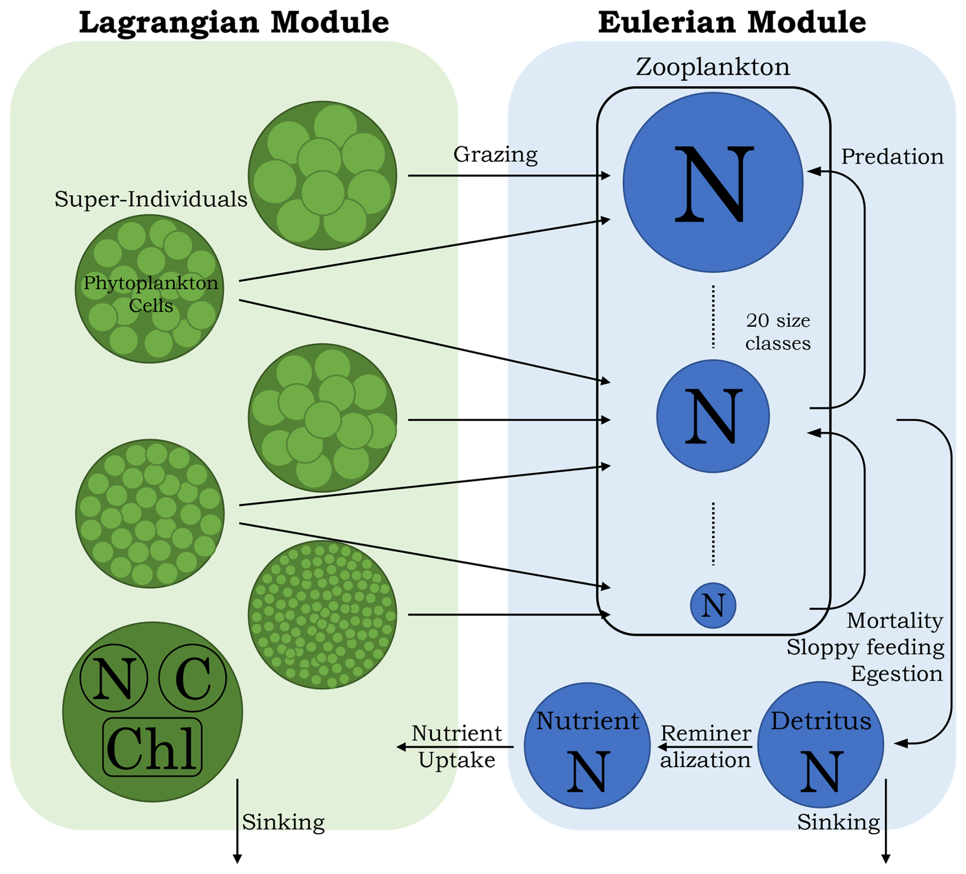
Figure 1 Conceptual diagram of the 1D PIBM model. N: nitrogen. C: carbon. Chl: chlorophyll. The black arrows represent nitrogen flows.

2 Model description

2.1 Overview

PIBM is a 1D Eulerian–Lagrangian hybrid system, written in FORTRAN 90, that extends the classic NPZD framework. In PIBM, phytoplankton cells are represented by super-individuals (see below) within the Lagrangian module, which is coupled to an Eulerian module. The Eulerian module calculates the dynamics of dissolved inorganic nitrogen, multiple size classes of zooplankton, and detritus as continuous concentrations across the vertical domain. While nitrogen is the model’s primary currency, the model also estimates the carbon and chlorophyll content of phytoplankton cells. The model structure is illustrated in Fig. 1, with all model parameters listed in Tables 1 and 2. The following subsections provide detailed descriptions of both modules.

2.2 Lagrangian module

2.2.1 Super-individuals

The Lagrangian module simulates the phytoplankton community using super-individuals, which represent clusters of identical phytoplankton cells. This approach allows us to model a realistic number of cells while keeping computational costs manageable (Scheffer et al., 1995). To avoid memory limitations, the number of super-individuals remains constant throughout the simulation.

2.2.2 Phytoplankton model

Phytoplankton physiological rates, such as growth and nutrient uptake, are determined by three master traits: cell size, optimal temperature, and light affinity. These rates vary over time and depth, responding not only to changes in the external environment (nutrient availability, temperature, and light) but also to changes in community composition (traits) (Geider et al., 1998; Ross and Geider, 2009). Cell size influences the ability of phytoplankton to take up inorganic nutrients and its vulnerability to zooplankton grazing. It is expressed as the maximal carbon content per cell (C_div, pmol C cell⁻¹), which reflects the phytoplankton size in terms of its maximum carbon content during the division phase. While actual cellular carbon content (P_C, pmol C cell⁻¹) fluctuates due to photosynthesis and respiration, nutrient uptake and grazing rates depend solely on C_div. This simplification ensures that these rates are not constantly recalculated due to changes in P_C and only change when C_div varies due to mutation. Optimal temperature (T_opt, °C) and light affinity, expressed as the initial slope of the photosynthesis-irradiance curve (α^Chl, m² mol C (W g Chl d)⁻¹), describe phytoplankton response to environmental temperature and light conditions.

We assign the three master traits to each phytoplankton super-individual at the beginning of the simulation, with values randomly drawn from a uniform distribution within predefined minimum and maximum limits. Once assigned, trait values remain constant throughout the simulation unless a mutation occurs (Sect. 2.2.3), which helps to sustain diversity.

At the heart of the Lagrangian module lie the equations governing phytoplankton cellular carbon (P_C), nitrogen (P_N, pmol N cell⁻¹), and chlorophyll (P_Chl, pg Chl cell⁻¹), formulated following Geider et al. (1998). Geider et al. (1998)'s equations describe the balance of photosynthesis, nutrient uptake, respiration, and chlorophyll synthesis, capturing how phytoplankton regulate their cellular contents in response to environmental conditions. Equation (1) states that phytoplankton cellular carbon is fueled by photosynthesis, which converts inorganic carbon into organic carbon, but is depleted by the cost of nutrient uptake and respiration. Equation (2) states that phytoplankton cellular nitrogen is fueled by nitrogen uptake but is depleted by respiration. Equation (3) states that phytoplankton cellular chlorophyll content is fueled by chlorophyll synthesis, which depends on both photosynthesis and nitrogen uptake, but is consumed by respiration.

$$\begin{array}{}\text{(1)}& {\displaystyle \frac{\mathrm{1}}{P_{\mathrm{C}}}}{\displaystyle \frac{\mathrm{d}{P}_{\mathrm{C}}}{\mathrm{d}t}}=P^{\mathrm{C}}-\mathit{\zeta }{V}_{\mathrm{N}}^{\mathrm{C}}-R_{\mathrm{C}}f\left(T\right)\text{(2)}& {\displaystyle \frac{\mathrm{1}}{P_{\mathrm{N}}}}{\displaystyle \frac{\mathrm{d}{P}_{\mathrm{N}}}{\mathrm{d}t}}={\displaystyle \frac{V_{\mathrm{N}}^{\mathrm{C}}}{Q^{\mathrm{N}}}}-R_{\mathrm{N}}f\left(T\right)\text{(3)}& {\displaystyle \frac{\mathrm{1}}{P_{\mathrm{Chl}}}}{\displaystyle \frac{\mathrm{d}{P}_{\mathrm{Chl}}}{\mathrm{d}t}}={\displaystyle \frac{{\mathit{\rho }}_{\mathrm{Chl}}{V}_{\mathrm{N}}^{\mathrm{C}}}{{\mathit{\theta }}^{\mathrm{C}}}}-R_{\mathrm{Chl}}f\left(T\right)\end{array}$$

P^C (d⁻¹) is the carbon-specific photosynthesis rate, ζ (mol C mol N⁻¹) is the cost of biosynthesis, $V_{\mathrm{N}}^{\mathrm{C}}$ (mol N mol C⁻¹ d⁻¹) is the nitrogen uptake rate, Q^N (mol N mol C⁻¹) is the cellular N:C ratio, ρ^Chl (dimensionless) is the fraction of phytoplankton carbon production that is devoted to chlorophyll synthesis, θ^C (g Chl mol C⁻¹) is the ratio of Chl synthesis to carbon fixation (representing phytoplankton acclimation to light variability). The size-dependent R_C, R_N, and R_Chl (d⁻¹) are degradation rate constants representing the loss of phytoplankton carbon, nitrogen, and chlorophyll, respectively (Eq. 14) (Wirtz, 2011). R_C accounts for maintenance respiration, while R_N and R_Chl represent intracellular remineralization and pigment degradation. f(T) is the function describing the temperature (T, K) dependence of phytoplankton metabolism, which is detailed in the temperature section below. It is important to note that we implicitly assume that P_C, P_N, and P_Chl are not affected by zooplankton grazing which only reduces the number of cells per super-individual.

P^C is a function of light availability as defined below:

$$\begin{array}{}\text{(4)}& P^{\mathrm{C}}=P_{\mathrm{m}}^{\mathrm{C}}\left[\mathrm{1}-e^{\left(\frac{-{\mathit{\alpha }}^{\mathrm{Chl}}{\mathit{\theta }}^{\mathrm{C}}I{A}^{\mathrm{\infty }}}{P_{\mathrm{m}}^{\mathrm{C}}}\right)}\right],\end{array}$$

where $P_{\mathrm{m}}^{\mathrm{C}}$ (d⁻¹) is the maximal carbon-specific photosynthesis rate, I (W m⁻²) is the irradiance, and A^∞ (dimensionless) is the term that accounts for photosynthetic photoinhibition (see Eq. 6). Although photoinhibition was not originally included in Geider et al. (1998), incorporating it is essential for capturing the decline in photosynthetic efficiency under overly strong irradiance for species that are adapted to low light levels (Moore et al., 1998; Han, 2002; Ross et al., 2011).

$P_{\mathrm{m}}^{\mathrm{C}}$ depends on intracellular nutrient status:

$$\begin{array}{}\text{(5)}& P_{\mathrm{m}}^{\mathrm{C}}={\mathit{\mu }}_{\mathrm{m}}{\displaystyle \frac{Q^{\mathrm{N}}-Q_{\min }^{\mathrm{N}}}{Q_{\max }^{\mathrm{N}}-Q_{\min }^{\mathrm{N}}}},\end{array}$$

where μ_m (d⁻¹) is the maximal specific growth rate, which varies with temperature under nutrient- and light-replete conditions (Eq. 10). $Q_{\max }^{\mathrm{N}}$ (mol N mol C⁻¹) is the maximal nitrogen-to-carbon ratio and $Q_{\min }^{\mathrm{N}}$ is the minimal nitrogen cell quota; both depend on cell size (Table 2). Here, we replaced the original $P_{\mathrm{ref}}^{\mathrm{C}}$ (maximal photosynthetic capacity at a reference temperature) from Geider et al. (1998) with μ_m which depends on both temperature and light traits as shown later.

To simulate the short-term responses of phytoplankton cells to potential high light stress when they are dispersed to the surface, we include photoinhibition into the phytoplankton model following previous studies (Han, 2002; Ross et al., 2011; Nikolaou et al., 2016). Photoinhibition decreases the photosynthesis rate due to D1 protein damage under high light, and is expressed as the fraction of open photosynthetic units (PSU) (Han, 2002; Nikolaou et al., 2016):

$$\begin{array}{}\text{(6)}& A^{\mathrm{\infty }}={\displaystyle \frac{\mathrm{1}}{\mathrm{1}+{\mathit{\sigma }}_{\mathrm{PSII}}I\mathit{\tau }+K{\mathit{\sigma }}_{\mathrm{PSII}}^{\mathrm{2}}{I}^{\mathrm{2}}\mathit{\tau }}}.\end{array}$$

σ_PSII (m² W⁻¹) is the effective absorption cross-section of photosystem II (PSII), parameterized as a power-law relationship with θ^C equal to σ_PSII=δ (θ^C)^κ (Nikolaou et al., 2016). Here, δ ((W m⁻²)⁻¹ (g Chl g C⁻¹)⁻¹) and κ (dimensionless) are the normalization and exponent constants, respectively, in the relationship between σ_PSII and θ^C (Table 1). τ (s) is the turnover time of the electron transfer chain and K (s⁻¹) is the ratio of damage to repair constants ($K=k_{\mathrm{d}}/k_{\mathrm{r}}$).

The tension between photodamage (k_d, dimensionless) and repair (k_r, s) of a PSU determines the fraction of open reaction centers and the abundance of D1 proteins (essential for repairing the PSII reaction center) at a given light level. To set up a trade-off between high-light adapted and low-light adapted ecotypes (Moore et al., 1998), we assume that k_r and α^Chl are negatively correlated. Thus, phytoplankton cells adapted to low-light (i.e., with larger α^Chl), have a reduced capability of photo-repair (i.e., smaller K) (Key et al., 2010). Conversely, phytoplankton cells adapted to high-light (larger K) are better able to cope with photoinhibition but are less efficient in absorbing photons under low light (smaller α^Chl). In addition, we consider the effect of nutrient status on their ability to perform photorepair, as nutrient limitation can jeopardize photosynthetic energy transfer efficiency (Herrig and Falkowski, 1989). Based on this, we propose the following relationship for k_r:

$$\begin{array}{}\text{(7)}& k_{\mathrm{r}}=a{\left({\displaystyle \frac{{\mathit{\alpha }}^{\mathrm{Chl}}}{b}}\right)}^v{\displaystyle \frac{Q^{\mathrm{N}}-Q_{\min }^{\mathrm{N}}}{Q_{\max }^{\mathrm{N}}-Q_{\min }^{\mathrm{N}}}},\end{array}$$

where $a=\mathrm{2}\times {\mathrm{10}}^{-\mathrm{5}}$, $b=\mathrm{5}\times {\mathrm{10}}^{-\mathrm{7}}$, and $v=-\mathrm{6.64}$ are constants. These parameters were obtained by fitting data from Prochlorococcus in Moore et al. (1998).

Phytoplankton nitrogen uptake ($V_{\mathrm{N}}^{\mathrm{C}}$) depends on both external dissolved inorganic nitrogen (DIN, mmol N m⁻³) levels and intracellular nitrogen status:

$$\begin{array}{}\text{(8)}& V_{\mathrm{N}}^{\mathrm{C}}=V_{\mathrm{m}}^{\mathrm{C}}{\displaystyle \frac{\mathrm{DIN}}{\mathrm{DIN}+K_{\mathrm{N}}}}{\left({\displaystyle \frac{Q_{\max }^{\mathrm{N}}-Q^{\mathrm{N}}}{Q_{\max }^{\mathrm{N}}-Q_{\min }^{\mathrm{N}}}}\right)}^n,\end{array}$$

where $V_{\mathrm{m}}^{\mathrm{C}}={\mathit{\mu }}_{\mathrm{m}}{Q}_{\max }^{\mathrm{N}}$ (mol N mol C⁻¹ d⁻¹) is the maximal specific nitrogen uptake rate, and K_N (mmol N m⁻³) is the half-saturation constant for DIN uptake. The parameter n (dimensionless), which varies between 0 and 1, determines the dependence of the maximum uptake rate ($V_{\mathrm{m}}^{\mathrm{C}}$) on cell quota (Q^N) (Geider et al., 1998). All three parameters – K_N, $Q_{\max }^{\mathrm{N}}$, and $Q_{\min }^{\mathrm{N}}$ – depend on cell size following allometric relationships (Table 2).

ρ^Chl (dimensionless) depends on light, photosynthetic rate, the initial slope of the photosynthesis-irradiance curve (α^Chl), and Chl:C ratio (θ^C):

$$\begin{array}{}\text{(9)}& {\mathit{\rho }}_{\mathrm{Chl}}={\mathit{\theta }}_{\max }^{\mathrm{N}}{\displaystyle \frac{P^{\mathrm{C}}}{{\mathit{\alpha }}^{\mathrm{Chl}}{\mathit{\theta }}^{\mathrm{C}}I}},\end{array}$$

where ${\mathit{\theta }}_{\max }^{\mathrm{N}}$ is the maximum chlorophyll-to-nitrogen ratio (g Chl mol N⁻¹). During dark hours, when I=0, ρ^Chl is assumed to retain the value calculated at the end of the preceding light period.

The maximal growth rate, μ_m, depends on T_opt (K) as well as the environmental temperature (T, K), following Chen (2022), which extends the Metabolic Theory of Ecology (Dell et al., 2011; Chen and Laws, 2017):

$$\begin{array}{}\text{(10)}& {\mathit{\mu }}_{\mathrm{m}}={\mathit{\mu }}_{\mathrm{0}}{\displaystyle \frac{E_{\mathrm{a}}+E_{\mathrm{d}}}{E_{\mathrm{d}}}}{\displaystyle \frac{e^{E_{\mathrm{a}}(x-\mathit{\theta })}}{\mathrm{1}+\frac{E_{\mathrm{a}}}{E_{\mathrm{d}}}{e}^{(E_{\mathrm{a}}+E_{\mathrm{d}})(x-\mathit{\theta })}}},\end{array}$$

where θ and x are the transformed optimal and environmental temperatures for mathematical convenience:

$$\begin{array}{}\text{(11)}& \mathit{\theta }={\displaystyle \frac{\mathrm{1}}{k_b}}\left({\displaystyle \frac{\mathrm{1}}{T_{\mathrm{0}}}}-{\displaystyle \frac{\mathrm{1}}{T_{\mathrm{opt}}}}\right),x={\displaystyle \frac{\mathrm{1}}{k_b}}\left({\displaystyle \frac{\mathrm{1}}{T_{\mathrm{0}}}}-{\displaystyle \frac{\mathrm{1}}{T}}\right),\end{array}$$

with T₀ (K) being the reference temperature set at 288 K. μ₀ (d⁻¹) is the normalization constant for μ_m at θ=0, E_a (eV) is the intraspecific activation energy, and E_d (eV) is the nominal activation energy regulating how fast the growth rate (μ, d⁻¹) decreases with increasing T when x>θ. Finally, k_b (eV K⁻¹) is the Boltzmann constant.

Based on the analysis of a dataset relating phytoplankton growth to temperature, μ₀ (d⁻¹), E_a (eV), and E_d (eV) are found to be allometric functions of θ (Chen, 2022):

$$\begin{array}{}\text{(12a)}& {\displaystyle }{\mathit{\mu }}_{\mathrm{0}}& {\displaystyle }={\mathit{\mu }}^{\prime }{e}^{E_{\mathrm{i}}\mathit{\theta }},\text{(12b)}& {\displaystyle }{E}_{\mathrm{a}}& {\displaystyle }=E_{\mathrm{a}\mathrm{0}}{e}^{\mathit{\beta }\mathit{\theta }},\text{(12c)}& {\displaystyle }{E}_{\mathrm{d}}& {\displaystyle }=E_{\mathrm{d}\mathrm{0}}{e}^{\mathit{\varphi }\mathit{\theta }},\end{array}$$

in which μ^′ (d⁻¹) is the normalization constant for μ₀ when θ=0, E_i (eV) is the interspecific activation energy, E_a0 (eV) is the normalization constant for E_a when θ=0, β (eV) is the scaling exponent against θ for E_a, E_d0 (eV) is the normalization constant for E_d when θ=0, and ϕ (eV) is the scaling exponent for E_d.

Following the mechanistic model of Wirtz (2011), we let μ^′ to decrease with cell equivalent spherical diameter (ESD, µm) as a result of intra-cellular self-shading and excess density:

$$\begin{array}{}\text{(13)}& {\mathit{\mu }}^{\prime }={\displaystyle \frac{{\mathit{\mu }}_{\mathrm{0}}^{\prime }}{\mathrm{1}+a_{\mathrm{0}}{\left(\frac{{\mathit{\rho }}^{\mathrm{s}}}{{\mathit{\rho }}_{\mathrm{0}}}\right)}^{\frac{\mathrm{1}}{\mathrm{3}}}\mathrm{ESD}}},\end{array}$$

where a₀ is the length scale of photosynthesis depletion. ${\mathit{\mu }}_{\mathrm{0}}^{\prime }$ is maximal potential growth rate (= 5 d⁻¹). ρ^s is the carbon density at a reference ESD (ESD_s=8.00 µm), and ρ₀ (=0.50 pg C m⁻³) is the specific carbon density for the relative chloroplast volume ($V_{\mathrm{Chl}}/V$).

We also consider that phytoplankton respiration (R_C, R_N, and R_Chl) follows the same temperature dependence as μ_m (Barton et al., 2020). Following Wirtz (2011), these specific respiration rates are assumed to scale inversely with phytoplankton ESD:

$$\begin{array}{}\text{(14)}& R_{*}=R_{*,s}{\displaystyle \frac{{\mathrm{ESD}}_s}{\mathrm{ESD}}},\end{array}$$

where $R_{*,\mathrm{s}}$ is the temperature-dependent respiration rate at ESD_s for carbon, nitrogen or chlorophyll. If T=T_opt, $R_{*,s}=\mathrm{0.1}$ d⁻¹ for the specific respiration rates of phytoplankton carbon, nitrogen, and chlorophyll.

Equations (13) and (14) capture the unimodal relationship between maximal growth rate and cell size (Chen and Liu, 2010, 2011; Marañón et al., 2013). If a phytoplankton cell is too large, its self-shading and intracellular decline of CO₂ reduces its maximal growth rate. On the other hand, if a cell is too small, the high specific respiration cost leads to a rapid decline in maximal growth rate. This tradeoff on the range of cell size plays a critical role in constraining phytoplankton size range in the model in which the phytoplankton cells are allowed to evolve freely by mutation. Without this tradeoff, phytoplankton will evolve towards infinitely small cells in very oligotrophic environments.

2.2.3 Phytoplankton division, mutation, and death

Phytoplankton cell division occurs when the cellular carbon content reaches C_div (Cianelli et al., 2009; Ross and Geider, 2009). Upon division, the parent cell is split into two equal daughter cells, each inheriting half of the carbon, nitrogen, and chlorophyll content. As a consequence, the number of cells per super-individual doubles. By default, the daughter cells inherit the same trait values for C_div, T_opt, and α^Chl as the parent cell; however, they have a small probability of mutation, with the trait values altered according to a Gaussian distribution with mean equal to the parent's value and a specified standard deviation. The probability of mutation for a super-individual (ν_j,phy) is proportional to its number of cells (n_j,phy), such that ${\mathit{\nu }}_{j,\mathrm{phy}}={\mathit{\nu }}_{\mathrm{0}}{n}_{j,\mathrm{phy}}$, where ν₀ represents the mutation rate per cell.

Although this mutation framework may not accurately reflect reality, for simplicity and ease of modeling, we assume that all ecotypes share the same mutation rate. However, in reality, mutation rates can vary among different phytoplankton ecotypes (Beardmore et al., 2011), and even within the same species when subjected to stress (Bjedov et al., 2003). Additionally, while we assume that the mutation of one trait is independent of others, the user can modify the mutation covariance matrix to change how the mutation of one trait depends on those of other traits.

Phytoplankton cells die when their cellular carbon content falls below a minimal threshold (C_min, pmol C cell⁻¹), defined as a quarter of C_div (Ross and Geider, 2009), or when the total nitrogen content of a super-individual drops below 0.10 % of the average nitrogen content of all super-individuals. It is important to note that in addition to respiratory cost, phytoplankton cells are subject to zooplankton grazing. We assume that zooplankton grazing can only reduce the number of cells per super-individual without affecting cellular carbon or nitrogen. When a cell dies, its nitrogen content is converted into detritus. Simultaneously, to maintain a constant number of super-individuals, the super-individual with the maximum nitrogen content is divided into two new super-individuals, each containing half of the cells of the parent

2.3 Eulerian module

Dynamics of dissolved inorganic nitrogen, zooplankton, and detritus are modeled as Eulerian fields.

2.3.1 Dissolved inorganic nitrogen

The temporal and spatial variability of dissolved inorganic nitrogen (DIN, mmol N m⁻³) is governed by several processes: the total nutrient uptake by phytoplankton (P_uptake, mmol N m⁻³; see Eq. 16), zooplankton excretion (Z_exc; see Eq. 17), detritus regeneration (D_reg; see Eq. 18), and vertical diffusion (the last term in Eq. 15):

$$\begin{array}{}\text{(15)}& {\displaystyle \frac{\partial \mathrm{DIN}}{\partial t}}=-P_{\mathrm{uptake}}+Z_{\mathrm{exc}}+D_{\mathrm{reg}}+{\displaystyle \frac{\partial }{\partial z}}\left[K_{\mathrm{v}}\right(z\left){\displaystyle \frac{\partial \mathrm{DIN}}{\partial z}}\right],\end{array}$$

where K_v(z) (m² s⁻¹) denotes the vertical eddy diffusivity at each depth layer. P_uptake in grid s over the time step Δt is defined as the sum of the nutrients taken up by all super-individuals within that grid:

$$\begin{array}{}\text{(16)}& \begin{array}{rl}{P}_{\mathrm{uptake}}& ={\displaystyle \frac{\mathrm{1}}{H\left(s\right)}}\sum _{i=\mathrm{1}}^k\\ & \left[\right(P_{\mathrm{N},i}(t+\mathrm{\Delta }t)-P_{\mathrm{N},i}\left(t\right)\left)n_i\right(t+\mathrm{\Delta }t\left)\right],\end{array}\end{array}$$

in which H(s) (m) is the height of the vertical grid s, $P_{\mathrm{N},i}(t+\mathrm{\Delta }t)$ and P_N,i(t) (mmol N per cell) represent the cellular nitrogen content of super-individual i at time t+Δt and t, respectively, and n_i(t+Δt) represents the number of cells associated with the super-individual i at time t+Δt.

We assume that Z_exc is a constant fraction of the total amount of food ingested by all zooplankton:

$$\begin{array}{}\text{(17)}& Z_{\mathrm{exc}}=(\mathrm{1}-\mathit{\xi }-\mathit{\eta })\sum _{j=\mathrm{1}}^{N_z}{I}_j{\mathrm{ZOO}}_j,\end{array}$$

where ξ (dimensionless) represents the gross growth efficiency of zooplankton and is assumed to be the same for each size class. N_z is the number of zooplankton size classes (=20). η (dimensionless) denotes the fraction of unassimilated food by zooplankton, also assumed the same for each size class. I_j (d⁻¹) is the per capita total ingestion rate of zooplankton in size class j, as detailed in the following section.

D_reg is a linear function of both detritus concentration (DET, mmol N m⁻³) and temperature (T, °C):

$$\begin{array}{}\text{(18)}& D_{\mathrm{reg}}=R_{\mathrm{dn}}\mathrm{DET}{f}_{\mathrm{h}}\left(T\right),\end{array}$$

where R_dn (d⁻¹) is the conversion rate of detritus into dissolved inorganic nitrogen, and f_h(T) describes the temperature dependence of heterotrophic activities, including zooplankton grazing and detritus regeneration, formulated according to the Arrhenius equation:

$$\begin{array}{}\text{(19)}& f_{\mathrm{h}}\left(T\right)=e^{\frac{E_z}{k_b}\left(\frac{\mathrm{1}}{T_{\mathrm{0}}}-\frac{\mathrm{1}}{T}\right)}=e^{E_{z}x},\end{array}$$

where E_z (eV) is the activation energy for heterotrophic processes (see Table 1).

2.3.2 Zooplankton

The code for modeling zooplankton biomass was developed drawing inspiration from the equations described by Ward et al. (2012). The model resolves 20 zooplankton size classes, spaced logarithmically from 0.80 to 3600 µm ESD. The smallest size class is set at 0.80 µm to represent the smallest heterotrophic eukaryotes in the ocean, which predominantly feed on bacteria. The upper limit of 3600 µm is chosen as a tradeoff between ensuring appropriate grazers for large phytoplankton and managing computational cost, as we fix the number of zooplankton size classes as 20. Because phytoplankton cells are free to evolve in size during the simulation, some may become so large (or small) that no zooplankton can feed on them. However, expanding the zooplankton size range too much would reduce the resolution size classes within the realistic zooplankton size range.

The nitrogen biomass of each zooplankton size class (ZOO_j, mmol N m⁻³) increases as they consume prey, including phytoplankton super-individuals and smaller zooplankton, but decreases due to predation by larger zooplankton and natural mortality.

$$\begin{array}{}\text{(20)}& \begin{array}{rl}{\displaystyle \frac{\partial {\mathrm{ZOO}}_j}{\partial t}}& ={\mathrm{ZOO}}_j{\mathit{\xi }}_j\sum _{j_{\mathrm{prey}}=\mathrm{1}}^J{I}_{j,j_{\mathrm{prey}}}\\ & -\sum _{j_{\mathrm{pred}}=\mathrm{1}+j}^{N_z}{\mathrm{ZOO}}_{j_{\mathrm{pred}}}{I}_{j_{\mathrm{pred}},j}-{\mathrm{ZOO}}_j{m}_z{f}_{\mathrm{h}}\left(T\right)\\ & +{\displaystyle \frac{\partial }{\partial z}}\left(K_{\mathrm{v}}\right(z\left){\displaystyle \frac{\partial {\mathrm{ZOO}}_j}{\partial z}}\right),\end{array}\end{array}$$

where m_z (d⁻¹) is the linear zooplankton mortality rate, and J is the total number of prey items, including phytoplankton super-individuals and smaller zooplankton within the grid.

Zooplankton per capita ingestion rate ($I_{j_{\mathrm{pred}},j_{\mathrm{prey}}}$, d⁻¹) is calculated using a sigmoidal functional response that depends on total prey biomass ($B_{j_{\mathrm{prey}}}$, mmol N m⁻³) (Ward et al., 2012):

$$\begin{array}{}\text{(21)}& I_{j_{\mathrm{pred}},j_{\mathrm{prey}}}=f_{\mathrm{h}}\left(T\right)I_{j_{\mathrm{pred}}}^{\max }{\displaystyle \frac{{\mathit{\varphi }}_{j_{\mathrm{pred}},j_{\mathrm{prey}}}{B}_{j_{\mathrm{prey}}}}{F_{j_{\mathrm{pred}}}+K_{P,j_{\mathrm{pred}}}}}(\mathrm{1}-e^{\mathrm{\Lambda }{F}_{j_{\mathrm{pred}}}}),\end{array}$$

where $I_{j_{\mathrm{pred}}}^{\max }$ (d⁻¹) is the size-dependent maximum ingestion rate (Table 2) (Hansen et al., 1997; Ward et al., 2012). ${\mathit{\varphi }}_{j_{\mathrm{pred}},j_{\mathrm{prey}}}$ (dimensionless) represents the palatability of prey j_prey for predator j_pred. $F_{j_{\mathrm{pred}}}$ (mmol N m⁻³) is the total prey availability for predator j_pred, and $K_{P,j_{\mathrm{pred}}}$ (mmol N m⁻³) is the grazing half-saturation constant of predator j_pred. The term (1−e^ΛF) accounts for the effect of prey refuge, which reduces grazing effort when available prey becomes scarce (Mayzaud and Poulet, 1978). The total ingestion rate of zooplankton size class j is therefore given by $I_j={\sum }_{j_{\mathrm{prey}}=\mathrm{1}}^J{I}_{j,j_{\mathrm{prey}}}$.

The food availability for zooplankton size class j_zoo ($F_{j_{\mathrm{zoo}}}$) includes both phyto- and zooplankton prey and is computed as

$$\begin{array}{}\text{(22)}& F_{j_{\mathrm{zoo}}}=\sum _{i_{\mathrm{phy}}=\mathrm{1}}^k{\mathit{\varphi }}_{j_{\mathrm{zoo}},i_{\mathrm{phy}}}{B}_{i_{\mathrm{phy}}}+\sum _{i_{\mathrm{zoo}}=\mathrm{1}}^{j_{\mathrm{zoo}}-\mathrm{1}}{\mathit{\varphi }}_{j_{\mathrm{zoo}},i_{\mathrm{zoo}}}{B}_{i_{\mathrm{zoo}}},\end{array}$$

where k is the number of super-individuals within the vertical grid. $B_{i_{\mathrm{phy}}}=n_{i_{\mathrm{Phy}}}{P}_{N,i_{\mathrm{Phy}}}/H$ and $B_{i_{\mathrm{zoo}}}$ (mmol N m⁻³) represent the nitrogen biomass of the $i_{\mathrm{Phy}}^{\mathrm{th}}$ phytoplankton super-individual and the $i_{\mathrm{zoo}}^{\mathrm{th}}$ zooplankton size class, respectively.

Since there is no zooplankton prey for the smallest zooplankton size class (j_zoo=1), we assume that zooplankton do not feed on other zooplankton larger than themselves but can feed on any phytoplankton prey. However, feeding on phytoplankton larger than their optimal prey size is penalized due to low prey palatability, ${\mathit{\varphi }}_{j_{\mathrm{pred}},j_{\mathrm{prey}}}$ (dimensionless):

$$\begin{array}{}\text{(23)}& {\mathit{\varphi }}_{j_{\mathrm{pred}},j_{\mathrm{prey}}}=\exp \left[-{\left(\ln \left({\displaystyle \frac{{\mathit{\vartheta }}_{j_{\mathrm{pred}},j_{\mathrm{prey}}}}{{\mathit{\vartheta }}_{\mathrm{opt}}}}\right)\right)}^{\mathrm{2}}{\left(\mathrm{2}{\mathit{\sigma }}_{j_{\mathrm{pred}}}^{\mathrm{2}}\right)}^{-\mathrm{1}}\right],\end{array}$$

where ${\mathit{\vartheta }}_{j_{\mathrm{pred}},j_{\mathrm{prey}}}$ (dimensionless) is the predator:prey volume ratio, ϑ_opt (dimensionless) is the optimal predator:prey volume ratio (Kiørboe, 2009), and ${\mathit{\sigma }}_{j_{\mathrm{pred}}}$ (dimensionless) is the standard deviation of the feeding kernel.

ϑ_opt is estimated based on the optimal prey size, which is defined by the relationship between ESD of the optimal prey (${\mathrm{ESD}}_{{\mathrm{prey}}_{\mathrm{opt}}}^{\mathrm{pred}}$) and the predator ESD (ESD_pred) (Hansen et al., 1994; Banas, 2011):

$$\begin{array}{}\text{(24)}& {\mathrm{ESD}}_{{\mathrm{prey}}_{\mathrm{opt}}}^{\mathrm{pred}}=\mathrm{0.65}{\mathrm{ESD}}_{\mathrm{pred}}^{\mathrm{0.56}}.\end{array}$$

As we assume that zooplankton grazing only affects the number of cells per super-individual ($n_{i_{\mathrm{phy}}}$) rather than cellular carbon or nitrogen, estimating changes in $n_{i_{\mathrm{phy}}}$ while conserving total nitrogen is not trivial. We assume that phytoplankton mortality due to zooplankton grazing (g_phy, d⁻¹), i.e., the proportional loss of nitrogen content during the time step Δt, is equal for all phytoplankton cells within the same super-individual and for all phytoplankton cells within the same vertical layer. While phytoplankton cell deaths can be modeled as a binomial process, the law of large numbers allows us to assume that the loss of cell numbers within a super-individual is proportional to the grazing rate g_phy (Beckmann et al., 2019). Therefore, we have

$$\begin{array}{}\text{(25)}& n_{i_{\mathrm{phy}}}(t+\mathrm{\Delta }t)=n_{i_{\mathrm{phy}}}\left(t\right)(\mathrm{1}-g_{\mathrm{phy}}\mathrm{\Delta }t).\end{array}$$

The total phytoplankton biomass loss due to zooplankton grazing within each vertical layer (P_G, mmol N m⁻³) is computed as follows (note that we drop the subscript of z for convenience):

$$\begin{array}{}\text{(26)}& \begin{array}{rl}{P}_{\mathrm{G}}& =-{\displaystyle \frac{\mathrm{1}}{H}}\sum _{i_{\mathrm{phy}}=\mathrm{1}}^k{P}_{\mathrm{N},i_{\mathrm{phy}}}\left(t\right)\left(n_{i_{\mathrm{phy}}}\right(t)-n_{i_{\mathrm{phy}}}(t+\mathrm{\Delta }t\left)\right)\\ & =-{\displaystyle \frac{\mathrm{1}}{H}}\sum _{i_{\mathrm{phy}}=\mathrm{1}}^k{P}_{\mathrm{N},i_{\mathrm{phy}}}\left(t\right)\left(n_{i_{\mathrm{phy}}}\right(t)-n_{i_{\mathrm{phy}}}(t\left)\right(\mathrm{1}-g_{\mathrm{phy}}\mathrm{\Delta }t\left)\right)\\ & =-{\displaystyle \frac{\mathrm{1}}{H}}\sum _{i_{\mathrm{phy}}=\mathrm{1}}^k{P}_{\mathrm{N},i_{\mathrm{phy}}}\left(t\right)n_{i_{\mathrm{phy}}}\left(t\right)g_{\mathrm{phy}}\mathrm{\Delta }t\\ & =g_{\mathrm{phy}}\mathrm{\Delta }t{\displaystyle \frac{{\sum }_{i_{\mathrm{phy}}=\mathrm{1}}^k{P}_{\mathrm{N},i_{\mathrm{phy}}}\left(t\right)n_{i_{\mathrm{phy}}}\left(t\right)}{H}}\\ & =\sum _{j_{\mathrm{zoo}}=\mathrm{1}}^{N_{\mathrm{Z}}}{I}_{j_{\mathrm{zoo}},i_{\mathrm{phy}}}\mathrm{\Delta }t,\end{array}\end{array}$$

where k is the number of phytoplankton super-individuals within the vertical layer.

Since $\frac{{\sum }_{i_{\mathrm{phy}}=\mathrm{1}}^k{P}_{\mathrm{N},i_{\mathrm{phy}}}\left(t\right)n_{i_{\mathrm{phy}}}\left(t\right)}{H}$ represents the total phytoplankton nitrogen concentration within each vertical layer (P_N), we can derive:

$$\begin{array}{}\text{(27)}& g_{\mathrm{phy}}={\displaystyle \frac{{\sum }_{j_{\mathrm{zoo}}=\mathrm{1}}^{N_{\mathrm{Z}}}{I}_{j_{\mathrm{zoo}},i_{\mathrm{phy}}}}{P_{\mathrm{N}}}}.\end{array}$$

Hence, the number of cells within a super-individual at the next time step (t+Δt) is given by

$$\begin{array}{}\text{(28)}& n_{i_{\mathrm{phy}}}(t+\mathrm{\Delta }t)=n_{i_{\mathrm{phy}}}\left(t\right)(\mathrm{1}-{\displaystyle \frac{{\sum }_{j_{\mathrm{zoo}}=\mathrm{1}}^{N_{\mathrm{Z}}}{I}_{j_{\mathrm{zoo}},i_{\mathrm{phy}}}}{P_{\mathrm{N}}}}\mathrm{\Delta }t).\end{array}$$

It is therefore important that the grazing effect ($n_{i_{\mathrm{phy}}}(t+\mathrm{\Delta }t)$) has to be computed before phytoplankton nutrient uptake (P_uptake, Eq. 16).

2.3.3 Detritus

Changes in the concentration of detritus (DET, mmol N m⁻³) are computed as

$$\begin{array}{}\text{(29)}& \begin{array}{rl}{\displaystyle \frac{\partial \mathrm{DET}}{\partial t}}& =\sum _{j=\mathrm{1}}^{N_z}(\mathit{\eta }{I}_j+m_{\mathrm{z}}{f}_{\mathrm{h}}(T\left)\right){\mathrm{ZOO}}_j\\ & -R_{\mathrm{dn}}\mathrm{DET}{f}_{\mathrm{h}}\left(T\right)-W_{\mathrm{d}}{\displaystyle \frac{\partial \mathrm{DET}}{\partial z}}\\ & +{\displaystyle \frac{\partial }{\partial z}}\left(K_{\mathrm{v}}\right(z\left){\displaystyle \frac{\partial \mathrm{DET}}{\partial z}}\right),\end{array}\end{array}$$

where W_d (m d⁻¹) is the detritus sinking rate.

2.3.4 Phytoplankton biomass and primary production

The Eulerian module also calculates the concentration of total phytoplankton nitrogen, carbon, and chlorophyll biomass, as well as the net primary productivity at each grid layer.

The concentration of total phytoplankton nitrogen, carbon, and chlorophyll biomass (B_*; $B_{{\mathrm{P}}_{\mathrm{N}}}$, mmol N m⁻³; $B_{{\mathrm{P}}_{\mathrm{C}}}$, mmol C m⁻³; and $B_{{\mathrm{P}}_{\mathrm{Chl}}}$, mg Chl m⁻³) is computed at each grid layer as follows (note that we drop the subscript of z for convenience):

$$\begin{array}{}\text{(30)}& B_{*}={\displaystyle \frac{{\sum }_{i=\mathrm{1}}^k{P}_{i_{\mathrm{phy}}}^{*}\cdot n_{i_{\mathrm{phy}}}}{H}},\end{array}$$

where $P_{i_{\mathrm{phy}}}^{*}$ represents the three different units of mass (i.e., P_N, P_C and P_Chl).

Net primary productivity (NPP, mg C m⁻³ d⁻¹) of a vertical layer is integrated over a daily cycle:

$$\begin{array}{}\text{(31)}& \mathrm{NPP}={\displaystyle \frac{\mathrm{1}}{H}}\sum _{t=\mathrm{0}}^{\mathrm{24}}\sum _{i=\mathrm{1}}^{k\left(t\right)}\left[\mathrm{\Delta }{P}_{\mathrm{C},i}\right(t\left)n_i\right(t\left)\right],\end{array}$$

where k(t) is the number of phytoplankton super-individuals at time t in that layer.

2.4 Physical forcing

As a case study, our 1D model simulates the upper 250 m of the Bermuda Atlantic Time-series Study (BATS) station. To maintain generality and simplicity, some region-specific details, such as phosphorus limitation instead of nitrogen limitation, are not included. The vertical grid consists of 100 levels, with resolution increasing toward the sea surface, following a sigma grid approach similar to that used in the Regional Ocean Modeling System (ROMS; Shchepetkin and McWilliams, 2005).

The model is externally forced by three environmental variables: temperature, vertical eddy diffusivity, and photosynthetically active radiation (PAR). Temperature profiles (T, °C) are prescribed from monthly climatological data in the World Ocean Atlas 2013 (Locarnini et al., 2024). Vertical eddy diffusivity (K_v, m² s⁻¹) is interpolated from daily outputs of a previous model simulation using a 1D general ocean turbulence model (GOTM) which uses the k∼ϵ turbulence model to compute K_v (Burchard et al., 1999; Bruggeman and Bolding, 2014; Le Gland et al., 2021). Finally, surface PAR (I₀, W m⁻²) is estimated dynamically at each time step as a function of mid-day light, time of day, and day length, following Anderson et al. (2015). Light attenuation within the water column (I_z, W m⁻²) is computed at each time step using the Beer–Lambert law, incorporating the effects of seawater and chlorophyll absorption:

$$\begin{array}{}\text{(32)}& I_z=I_{\mathrm{0}}{e}^{-z\left(K_{\mathrm{w}}+K_{\mathrm{Chl}}{\int }_z^{\mathrm{0}}\mathrm{Chl}\left(z\right)\mathrm{d}z\right)},\end{array}$$

where K_w (m⁻¹) and K_Chl (m² (mg Chl)⁻¹) are the light attenuation coefficients for seawater and chlorophyll-a, respectively.

Figure 2 shows the seasonal evolution of the physical forcing variables, illustrating the typical temporal and spatial variability at the BATS station. During winter and early spring, temperatures remain low, while K_v is high. The mixed layer depth (MLD, m), defined as the depth where $K_{\mathrm{v}}<{\mathrm{10}}^{-\mathrm{4}}$ m² s⁻¹, reaches its maximum depth (∼ 250 m) from February to late March. From April onward, MLD decreases abruptly, coinciding with a reduction in K_v and a warming of the surface water. Throughout late spring and summer, the water column becomes strongly stratified, with the surface mixed layer warming and deepening to 50 m by September. At the onset of fall, cooling temperatures and increasing K_v deepen the surface mixed layer once again.

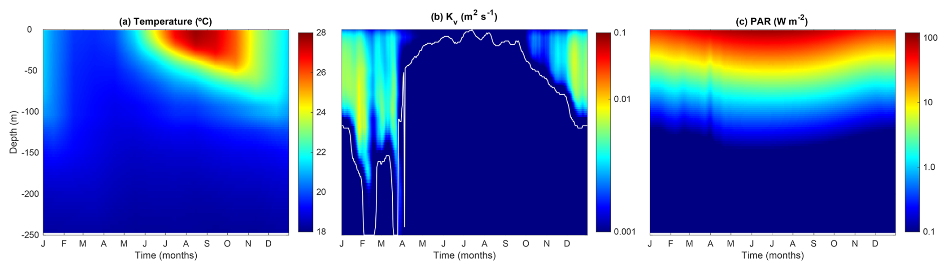
Figure 2 Temporal and vertical variability of the model forcing variables. (a) Temperature (°C), (b) vertical diffusivity (K_v, m² s⁻¹), and (c) photosynthetically active radiation (PAR; W m⁻²). In (b), the white line identifies the mixed layer depth (m).

2.5 Vertical transport of particles

In addition to the super-individuals, the Lagrangian module also simulates the movement of passive inert particles as a validation tool. Both passive particles and super-individuals move due to vertical diffusion, following a random walk model based on Visser (1997). The change in position (z_t) of an individual particle, from depth at time t to time t+1 (z_t+1), is computed over a finite time step δt as

$$\begin{array}{}\text{(33)}& \begin{array}{rl}{z}_{t+\mathrm{1}}& =z_t+K_{\mathrm{v}}^{\prime }\left(z_t\right)\mathit{\delta }t\\ & +R\sqrt{\mathrm{2}{r}^{-\mathrm{1}}{K}_{\mathrm{v}}(z_t+{\displaystyle \frac{\mathrm{1}}{\mathrm{2}}}{K}_{\mathrm{v}}^{\prime }(z_t\left)\mathit{\delta }t\right)\mathit{\delta }t},\end{array}\end{array}$$

where $K_{\mathrm{v}}^{\prime }\left(z_t\right)$ represents the vertical diffusion gradient ($=\mathit{\delta }{K}_{\mathrm{v}}/\mathit{\delta }z$) at depth z_t and R is a random variable drawn from a uniform distribution with zero mean and variance r ($r=\frac{\mathrm{1}}{\mathrm{3}}$ for a uniform distribution between −1 and 1) (Ross and Sharples, 2004).

In addition to diffusion, phytoplankton vertical movement is also influenced by sinking, which is size-dependent and follows the allometric relationship described in Durante et al. (2019) (Table 2). However, we assume no vertical current velocity in the system.

2.6 Initial conditions

In our standard model run, we initialize 20 000 phytoplankton super-individuals and 1000 passive particles with these numbers maintaining constant during the simulation. The vertical positions of both passive particles and phytoplankton super-individuals were randomly assigned between the surface (0 m) and bottom (250 m) at the start of the simulation, following a uniform distribution.

As previously explained, the three master traits were assigned to each phytoplankton super-individual at the beginning of the simulation. The initial ESD of each phytoplankton super-individual was randomly drawn from a uniform distribution in log space between 0.80 and 60.00 µm. These ESD values were then converted to phytoplankton cellular carbon content following Menden-Deuer and Lessard (2000) (Table 2). Subsequently, the initial cellular nitrogen content was estimated based on the Redfield ratio (C:N = $\mathrm{106}:\mathrm{16}\mathrm{mol}:\mathrm{mol}$), while the initial cellular chlorophyll content was calculated assuming a Chl:C ratio of 1:50 (g:g). C_div, the maximum carbon content at which a division event occurs, was set to twice the initial cellular carbon content. The initial number of phytoplankton cells per super-individual was calculated assuming a constant phytoplankton nitrogen concentration of 0.10 mmol m⁻³ throughout the water column.

T_opt values were randomly drawn from a uniform distribution between 2 and 30 °C. Similarly, α^Chl values were randomly drawn from a uniform distribution in log space between 0.01 and 0.50 m² mol C (W g Chl d)⁻¹.

In the Eulerian module, the initial concentrations of DIN were interpolated from the January profile at BATS, obtained from the World Ocean Atlas (Garcia et al., 2024). The total initial zooplankton nitrogen concentration was set to 0.10 mmol N m⁻³ throughout the water column and evenly distributed among the 20 size classes. Detritus concentration was also initialized as 0.10 mmol N m⁻³.

2.7 Boundary conditions

To preserve total nitrogen, zero fluxes are applied at both surface and bottom boundaries for all Eulerian fields. Additionally, a reflective boundary condition is used for particles encountering both surface and bottom boundaries during the random walk. We leave the option to use the Dirichlet boundary condition if one wishes to.

2.8 Model simulations

To achieve (quasi) steady-state seasonal cycles, PIBM was run for 6 years, with only the last year analyzed in this study. The model solves the differential equations governing biological processes using the forward Euler method with a constant 10 min time step. However, because the vertical random walk requires a shorter time step (Ross and Sharples, 2004), particles undergo 200 substeps per biological time step, resulting in a random walk time step of 3 s.

Due to the computational intensity of the particle random walk, we implemented parallel computing using the MPI standard, which can be compiled with different implementations such as Open MPI (Message Passing Interface Forum, 2023).

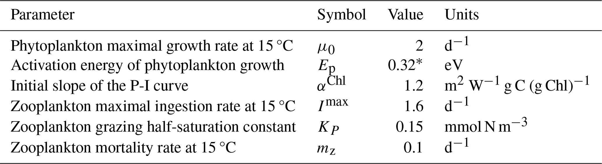
Table 1 Fixed parameters of the 1D PIBM model.

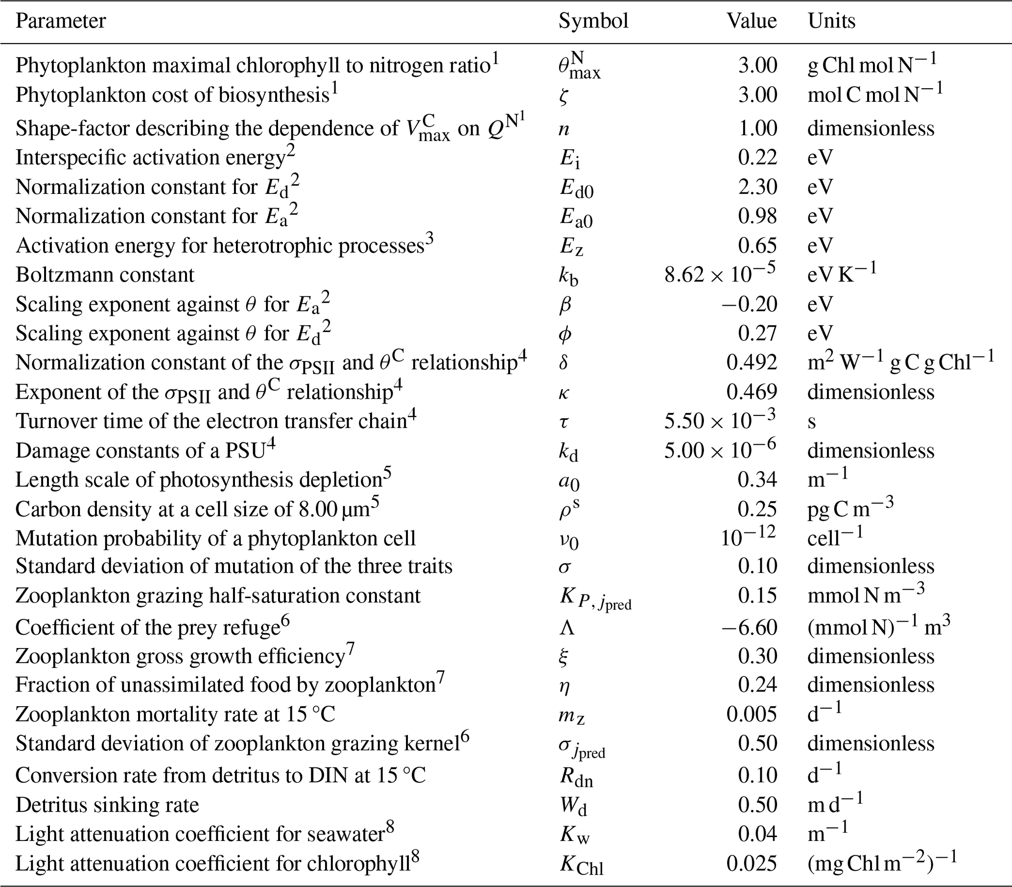
¹ Geider et al. (1998). ² Chen (2022). ³ Brown et al. (2004). ⁴ Nikolaou et al. (2016). ⁵ Wirtz (2011). ⁶ Ward et al. (2012). ⁷ Buitenhuis et al. (2010). ⁸ Gan et al. (2010).

Table 2 Size scaling coefficients for phytoplankton and zooplankton traits, following the general formula (y=aV^b), where V represents cell volume (µm³). For phytoplankton, V is derived from C_div using the allometric relationship from Marañón et al. (2013) (first entry in this table). For the size scaling of maximal phytoplankton growth and respiration rates, see Eqs. (13) and (14).

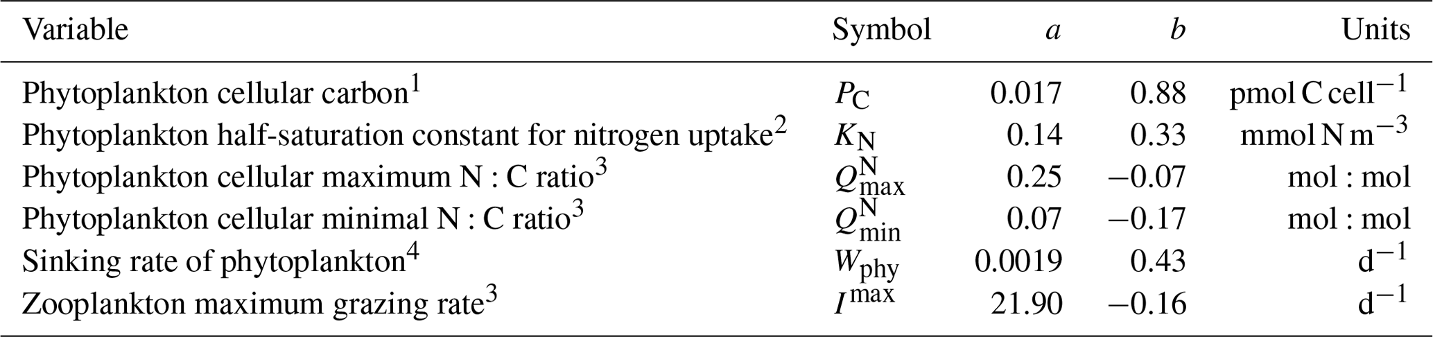
¹ Marañón et al. (2013). ² Edwards et al. (2012). ³ Ward et al. (2012). ⁴ Durante et al. (2019).

2.9 Observational data

For model validation, we obtained observational data for DIN (nitrate and nitrite), Chl, and NPP from the BATS website (https://bats.bios.asu.edu/, last access: 19 May 2024). To interpolate the data for each vertical grid at each time point, we applied the k-nearest neighbors (KNN) algorithm, with each data point calculated as the mean of the three nearest neighbors.

2.10 Mean trait and trait (co)variance

We characterize phytoplankton community composition in terms of mean trait values and trait (co)variance. Trait (co)variance serves as a measure of functional diversity, capturing trait variations in the community (Norberg et al., 2001; Chen et al., 2019; Le Gland et al., 2021). The community mean phytoplankton trait is calculated as the carbon-weighted mean of all phytoplankton cells in the community:

$$\begin{array}{}\text{(34)}& \stackrel{\mathrm{‾}}{l}={\displaystyle \frac{{\sum }_{i=\mathrm{1}}^k{l}_i{n}_i{P}_{\mathrm{C},i}}{{\sum }_{i=\mathrm{1}}^k{n}_i{P}_{\mathrm{C},i}}},\end{array}$$

where l_i and n_i represent the trait value and number of cells of super-individual i, respectively, and P_C,i represents the cellular carbon content of this super-individual.

The trait covariance is calculated as

$$\begin{array}{}\text{(35)}& \mathrm{COV}(l_j,l_m)={\displaystyle \frac{{\sum }_{i=\mathrm{1}}^k(l_{j,i}-\stackrel{\mathrm{‾}}{l_j})(l_{m,i}-\stackrel{\mathrm{‾}}{l_m})n_i{P}_{\mathrm{C},i}}{{\sum }_{i=\mathrm{1}}^k{n}_i{P}_{\mathrm{C},i}}},\end{array}$$

where $\stackrel{\mathrm{‾}}{l_j}$ and $\stackrel{\mathrm{‾}}{l_m}$ represent the mean values of trait j and m, respectively. l_j,i and l_m,i represent the trait j and m of super-individual i, respectively. It is important to note that we treat log (C_div), T_opt, and log (α^Chl) as traits as they are more likely to follow normal distribution than the raw units.

2.11 Functional diversity: Rao index

We computed the functional diversity of a phytoplankton community using the Rao index, a classic index to quantify diversity in functional ecology (Rao, 1982; De Bello et al., 2021):

$$\begin{array}{}\text{(36)}& \mathrm{Rao}=\sum _{i=\mathrm{1}}^{\mathrm{N}}\sum _{j=\mathrm{1}}^{\mathrm{N}}{p}_i{p}_j{d}_{ij},\end{array}$$

where p_i and p_j represent the relative proportion in carbon biomass of super-individual i and j, respectively, in the community. d_ij represents the Euclidean distance between these two super-individuals in the three-dimensional trait space:

$$\begin{array}{}\text{(37)}& d_{ij}=\sqrt{\sum _{k=\mathrm{1}}^{\mathrm{3}}(l_{i,k}^{\prime }-l_{j,k}^{\prime }{)}^{\mathrm{2}}},\end{array}$$

where $l_{i,k}^{\prime }$ represents the kth trait of super-individual i normalized between 0 and 1 because the three traits have different units ($l_{i,k}^{\prime }=\frac{l_{i,k}-l_{\min }}{l_{\max }-l_{\min }}$).

As shown above, the Rao index not only captures the relative abundance (biomass in this case) of each individual, but also takes into account trait similarities between individuals.

2.12 Size spectra

Size spectra have been widely used to provide insights into the size structure and energy flow of aquatic communities (Platt and Denman, 1977). To illustrate how this model can be used to simulate the plankton size distribution, we plotted the size spectra for both phyto- and zooplankton at the first 10 m of the water column and compared them between winter (20 February) and summer (20 August). We constructed the size-abundance spectra by calculating the total cell abundances in each of the 20 size bins that cover the entire size range of the simulated plankton community (from ∼ 0.80 to 3600 µm). The size bins were defined according to an octave (log₂) scale of cell volume.

The size-abundance spectra for phytoplankton is computed straightforwardly, with cellular volume derived using the allometric relationship between volume and cellular carbon (C_div, see Table 2). Each super-individual is assigned to the corresponding size bin based on its cellular volume, and the total abundance within each size bin is determined by summing the number of phytoplankton cells within all super-individuals of that volume range.

For zooplankton, the biovolume of each of the 20 size classes is known, but their abundance must be estimated from biomass concentration. Specifically, the abundance of each size class is estimated as the ratio of total zooplankton carbon biomass to the individual carbon content. To calculate individual carbon content, zooplankton nitrogen content is first converted to carbon for each size class using the canonical Redfield ratio (C:N = 106:16). The individual carbon content (Z_C, g C) is then derived from biovolume using the allometric relationship proposed by Harris et al. (2000):

$$\begin{array}{}\text{(38)}& Z_{\mathrm{C}}={\mathit{\rho }}_{\mathrm{Z}}{\displaystyle \frac{\mathit{\pi }}{\mathrm{6}}}{\mathrm{ESD}}^{\mathrm{3}}{p}_{\mathrm{d}}{p}_{\mathrm{c}},\end{array}$$

where ρ_Z (g cm⁻³) is the density of zooplankton, assumed to be equal to seawater density (1.025 g cm⁻³), p_d (dimensionless) is the proportion of wet mass composed of dry mass, and p_c (dimensionless) is the proportion of dry mass composed of carbon. For non-gelatinous zooplankton, we adopted values of p_d=0.20 and p_c=0.45.

The size spectra of both phytoplankton and zooplankton were calculated as ordinary least-squares regression lines with log₁₀-transformed total cell abundance (y-axis, individuals m⁻³) as the response variable and log₁₀-transformed cell volume for each size class (x-axis, µm³) as the predictor. All zero-abundance data were removed. Additionally, the abundance data of the two smallest size classes (0.80 µm, 1.20 µm) were removed for the zooplankton fraction because such small size classes, which deviate from the normal linear trend, were not often considered in the construction of size spectra.

2.13 Sensitivity analysis

2.13.1 Number of phytoplankton super-individuals

The number of phytoplankton super-individuals is a crucial parameter affecting the computation speed of PIBM. Ideally, we aim to determine the minimum number of super-individuals that can be used without compromising model accuracy. To assess the impact of the number of phytoplankton super-individuals on model outputs, we ran simulations with 5000, 10 000, and 50 000 super-individuals while keeping all other parameters constant and compared their results against the standard run with 20 000 super-individuals.

2.13.2 Comparison with simple NPZD models

To examine the effects of increased model complexity proposed in the PIBM, and assess how incorporating multiple phytoplankton traits influences plankton biomass and production, we implemented two simple NPZD models: one Eulerian and one Lagrangian. These models contain only a single, generic phytoplankton group, where carbon, nitrogen, and chlorophyll dynamics follow Geider et al. (1998) (Eqs. 1, 2, 3).

However, important differences exist. First, the term of photoinhibition is not included, meaning that P^C is an increasing function of light (I) in both models:

$$\begin{array}{}\text{(39)}& P^{\mathrm{C}}=P_{\mathrm{m}}^{\mathrm{C}}\left[\mathrm{1}-e^{\left(\frac{-{\mathit{\alpha }}^{\mathrm{Chl}}{\mathit{\theta }}^{\mathrm{C}}I}{P_{\mathrm{m}}^{\mathrm{C}}}\right)}\right].\end{array}$$

Second, μ_m is an exponential function of temperature following the Arrhenius equation:

$$\begin{array}{}\text{(40)}& {\mathit{\mu }}_{\mathrm{m}}={\mathit{\mu }}_{\mathrm{0}}{e}^{E_{\mathrm{p}}x},\end{array}$$

where E_p is the activation energy of phytoplankton.

Table 3 Parameters of the simple NPZD model that differ from PIBM.

^* Chen et al. (2012).

Last, there is only one zooplankton group that feeds exclusively on phytoplankton and experiences linear mortality:

$$\begin{array}{}\text{(41)}& \begin{array}{rl}{\displaystyle \frac{\partial \mathrm{ZOO}}{\partial t}}& =f_{\mathrm{h}}\left(T\right)\mathit{\xi }\mathrm{ZOO}{I}^{\max }{\displaystyle \frac{P_{\mathrm{N}}}{P_{\mathrm{N}}+K_{\mathrm{P}}}}(\mathrm{1}-e^{\mathrm{\Lambda }{P}_{\mathrm{N}}})\\ & -\mathrm{ZOO}{m}_{\mathrm{z}}{f}_{\mathrm{h}}\left(T\right)+{\displaystyle \frac{\partial }{\partial z}}\left(K_{\mathrm{v}}\right(z\left){\displaystyle \frac{\partial {\mathrm{ZOO}}_j}{\partial z}}\right).\end{array}\end{array}$$

We ran these two simple NPZD models under the same forcing as PIBM with identical simulation settings (e.g., time step, simulation duration). However, we have to stress that strict comparisons between PIBM and simpler NPZD models are impossible due to different parameter sets and model architecture.

3 Results

Below, we first describe the behavior of the phytoplankton model, followed by a detailed analysis of PIBM outputs. We then compare the modeled fields of DIN, Chl, and NPP against observations to ensure that our model can qualitatively reproduce the main observed patterns. Afterwards, we highlight patterns emerging from the model that may be interesting but hard to directly measure in situ. Finally, we present the results of sensitivity analyses, including the effects of phytoplankton super-individuals and comparisons against simple NPZD models.

3.1 Phytoplankton fitness landscapes

Figure 3 illustrates how growth rate (μ, d⁻¹) (top row), N:C (mol:mol) (middle row), and the Chl:C ratio (g:g) (bottom row) vary for different phytoplankton ecotypes which have unique combinations of traits (i.e., C_div, T_opt and α^Chl). To facilitate interpretation, we present 2D contour plots that vary two traits at a time (i.e., ESD vs. T_opt, ESD vs. α^Chl, and T_opt vs. α^Chl), while keeping the third trait constant. Figure 3 shows the results for the summer period, characterized by a constant DIN concentration of 0.10 mmol m⁻³, a temperature of 28 °C, and an irradiance of 250 W m⁻².

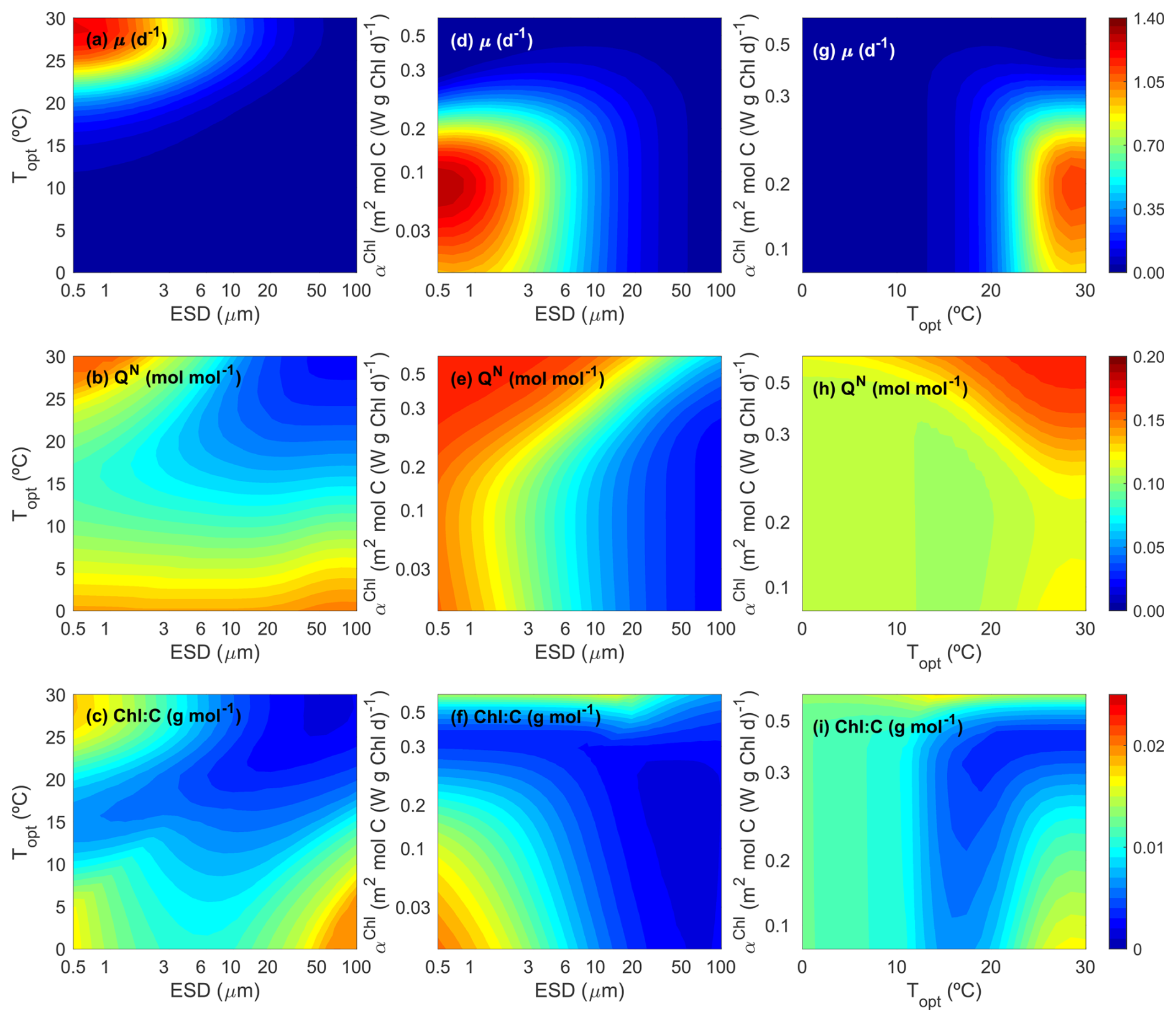
Figure 3 Contour plots for phytoplankton growth rate (μ, d⁻¹), N:C ratio (Q^N, mol:mol), and Chl:C ratio (g:g) as functions of the three master traits (size, ESD (µm); optimal temperature, T_opt (°C); and light affinity, α^Chl (m² mol C (W g Chl d)⁻¹)) at equilibrium under a typical summer condition (dissolved inorganic nitrogen = 0.10 mmol N m⁻³, temperature =28 °C, and PAR = 250 W m⁻²).

In the left column, we present the impact of cell size and T_opt, with a constant α^Chl of 0.08 m² mol C (W g Chl d)⁻¹. This α^Chl value is designed to adapt to the current light conditions without strong photoinhibition. As anticipated, the maximum peak of μ is observed for small-size phytoplankton (<3 µm), efficient at taking up nitrogen at low environmental concentrations, and with a T_opt around 28–30 °C, close to the environmental temperature (Fig. 3a). Moreover, we observe close to zero μ values for the whole size range when T_opt is far from the environmental temperature, highlighting maladapted ecotypes. N:C shows maximum values for small phytoplankton cells, almost regardless of T_opt (Fig. 3b), decreasing towards largest sizes, consistent with the observations by Baer et al. (2017). In this particular scenario, where both irradiance and α^Chl are constant, the Chl:C ratio also peaks for small cells with high T_opt (Fig. 3c), similar to μ. The increase in the Chl:C ratio for large-size ecotypes and T_opt<10 °C may be related to the minimum growth in carbon content (Fig. 3a).

In the middle column, we present how growth, N:C and Chl:C ratios change with cell size and α^Chl, with a constant T_opt of 30 °C. This T_opt value is close to the environmental temperature (28 °C), indicating adaptation to the ambient temperature. μ peaks for small phytoplankton (<3 µm) and α^Chl around 0.10 m² mol C (W g Chl d)⁻¹ (Fig. 3d). The light condition of 250 W m⁻² favor organisms with low light affinity values (α^Chl<0.20 W⁻¹ m² g Chl⁻¹ mol C d⁻¹) with high capability of photo-repair. N:C mainly depends on cell size, progressively decreasing towards the largest sizes (Fig. 3e). All else being equal, cells with more optimal α^Chl values tend to exhibit lower N:C ratios (Fig. 3e). Chl:C ratio shows the maximum values for the smallest phytoplankton with the lowest α^Chl, and the minimum values for the largest phytoplankton with the highest α^Chl (Fig. 3f). As larger α^Chl increases the probability of photoinhibition and reduces the carbon-specific photosynthesis rate, the amount of cellular chlorophyll content also decreases relative to carbon.

In the right column, we present the impact of T_opt and α^Chl, with a constant ESD of 1.36 µm. As anticipated, given the defined environmental conditions, the highest growth rate (μ) is achieved by phytoplankton cells with a T_opt close to the environmental temperature and α^Chl values around 0.10 W⁻¹ m² g Chl⁻¹ mol C d⁻¹, which are better adapted to high irradiance (Fig. 3g). Moreover, N:C increases with T_opt, with a minimum corresponding to cells with high growth (Fig. 3h). Similarly, the Chl:C ratio is maximized for ecotypes with T_opt closer to the environmental temperature and characterized by lower α^Chl values, resulting in reduced photoinhibition (Fig. 3i).

3.2 Comparisons with observations

We compared the observed DIN, Chl, and NPP at the BATS station with the model output (Fig. 4). Our model is able to reproduce the general qualitative patterns of these three variables, albeit with some quantitative differences. Both the observation and the model output show an increase in surface DIN and Chl during the winter when mixing is the strongest (Fig. 2). The model also successfully reproduces the deep chlorophyll maximum between 50 and 100 m. Despite the presence of the deep chlorophyll maximum, the model can reproduce the surface maximum of NPP, which extends below 50 m during the summer. Admittedly, there are some differences between the model output and the observations. The model appears to underestimate DIN in deep waters and overestimate Chl in the euphotic zone.

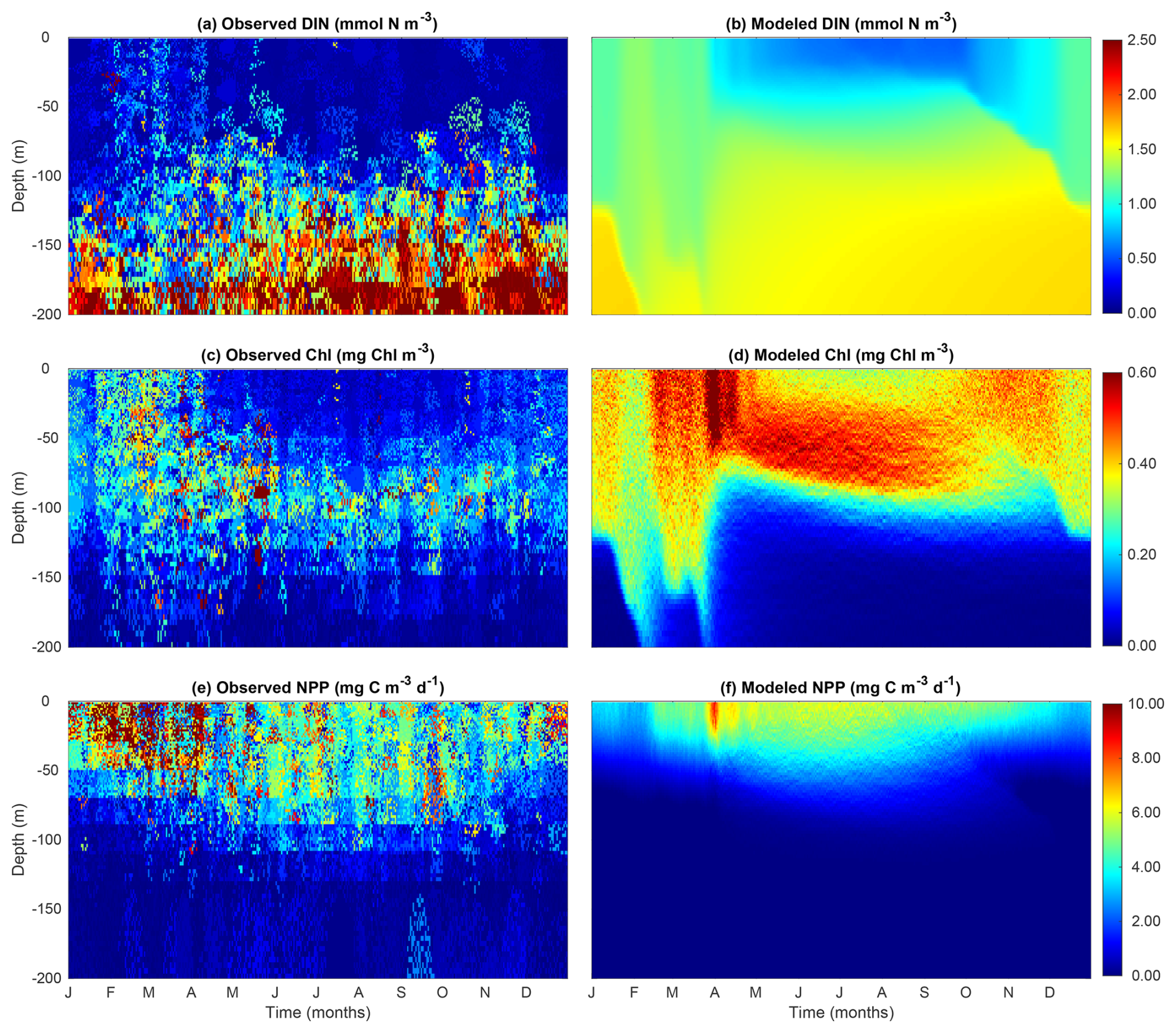
Figure 4 Daily comparison between observed data (a, c, e) and modeled data (b, d, f) for (a, b) dissolved inorganic nitrogen (DIN, mmol m⁻³), (c, d) chlorophyll concentration (Chl, mg m⁻³), and (e, f) net primary productivity (NPP, mg C m⁻³ d⁻¹).

3.3 Modeled patterns of passive particles

Figure 5 compares the vertical distribution of passive particles and phytoplankton super-individuals, allowing us to verify whether the Lagrangian module accurately represents the random walk of particles. While the distribution of phytoplankton super-individuals can be additionally affected by cell division and death, the distribution of passive particles is driven purely by diffusion.

As passive particles (Fig. 5a) are homogeneously distributed throughout the water column, we can affirm that the particle random walks are working correctly. During periods of high vertical mixing, the distribution of super-individuals shows a homogeneous pattern (Fig. 5b). However, as expected, during the period of strong stratification of the water column (April–October), more pronounced differences were observed. A greater number of super-individuals were found in the euphotic layer, where conditions for survival are optimal, with their abundance decreasing in deeper layers.

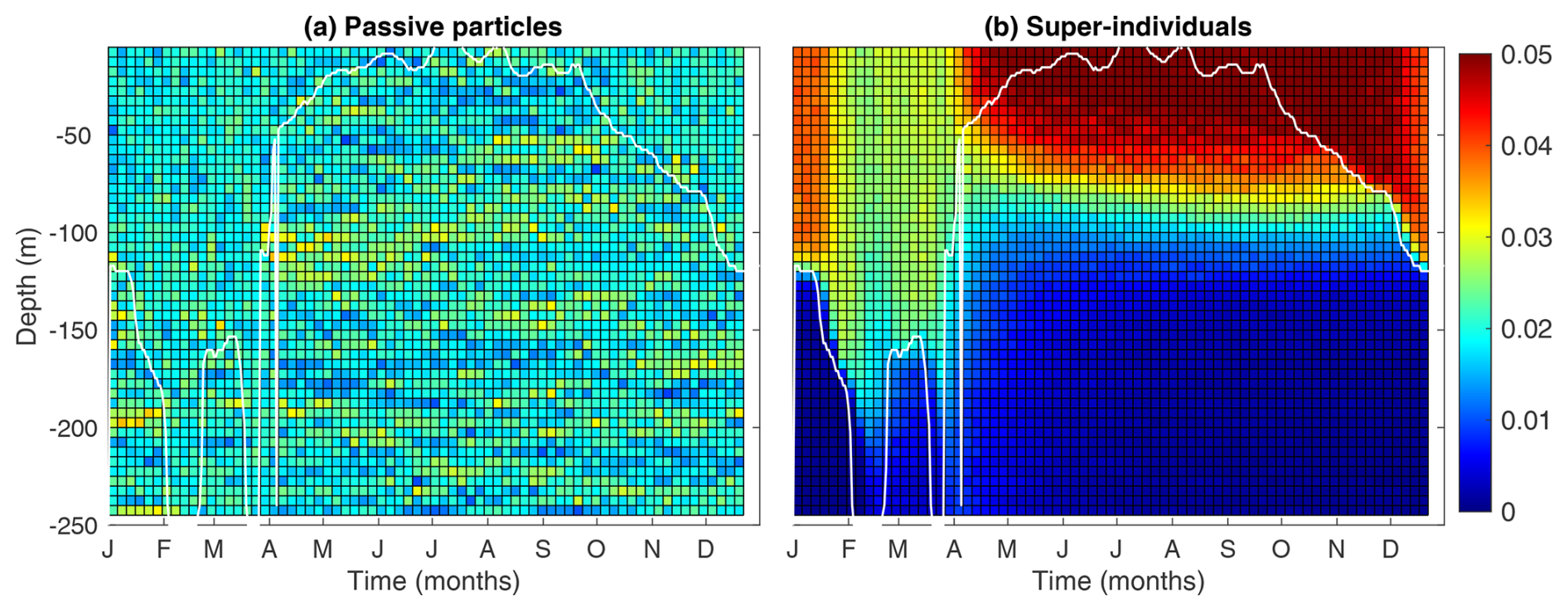
Figure 5 Mean temporal and vertical frequencies of (a) passive particles and (b) phytoplankton super-individuals every 5 m depth and every 5 d along the last year's simulation. The white lines represent the mixed layer depth (MLD, m).

3.4 Modeled patterns of phytoplankton carbon, nitrogen, zooplankton and detritus

Phytoplankton carbon and nitrogen concentrations, for which no observational data are available, show similar patterns. Both of them peak at spring after the shoaling of the mixed layer depth (Fig. 6a, b). Before the spring bloom, surface phytoplankton carbon and nitrogen can penetrate deeper than 150 m due to strong winter mixing. Similar to the patterns of chlorophyll, phytoplankton carbon also shows elevated concentrations at the deep chlorophyll maximum during summer, although this maximal layer is not as pronounced as that of chlorophyll (Fig. 4d).

By contrast, zooplankton biomass peaks in the summer and autumn after the phytoplankton spring bloom (Fig. 6c), suggesting that the demise of the phytoplankton spring bloom is at least attributed to intensified zooplankton grazing. Detritus also peaks after the phytoplankton spring bloom, but unlike zooplankton, its concentration gradually declines with time, as a result of both accelerated decomposition due to high temperature and shifts in zooplankton size structure.

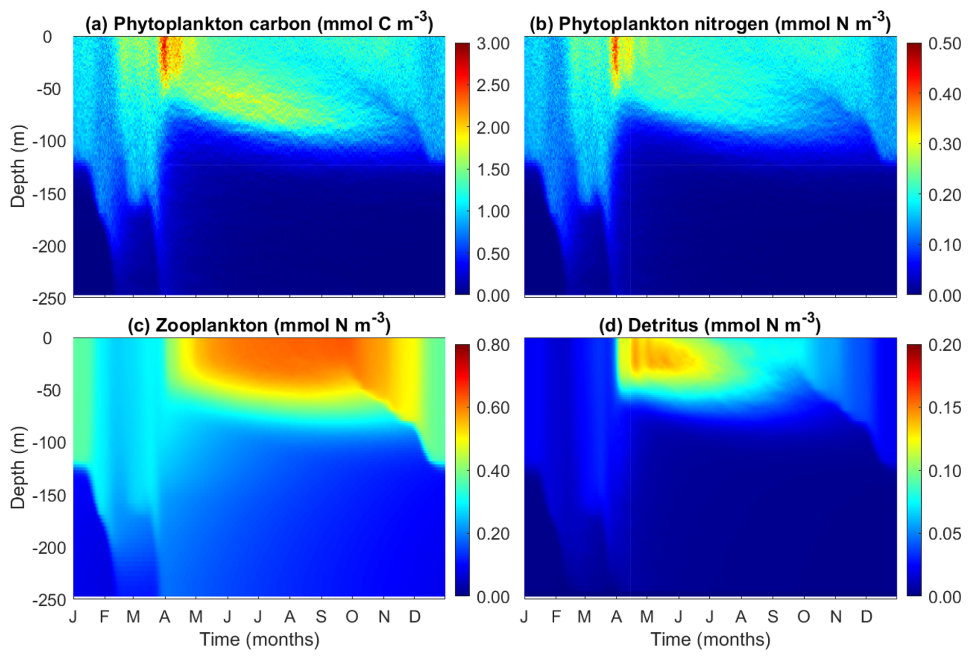
Figure 6 Temporal and vertical variability of modeled (a) phytoplankton carbon (mmol C m⁻³), (b) phytoplankton nitrogen (mmol N m⁻³), (c) total zooplankton nitrogen (mmol N m⁻³), and (d) detritus (mmol N m⁻³).

3.5 Modeled Chl:C and N:C ratios

The phytoplankton cellular N:C and Chl:C ratios are key indicators of how phytoplankton acclimate to light and nutrient availability. These ratios are also crucial for linking phytoplankton carbon to satellite-derived chlorophyll observations and to the limiting nutrient, nitrogen (Fig. 7).

The model predicts higher Chl:C ratios in the surface mixed layer during winter due to enhanced nutrient supply from strong mixing. In contrast, Chl:C ratios are lower in both the summer surface layer and in deep waters below the mixed layer. These patterns can be understood as an outcome of the balance between photosynthesis and chlorophyll synthesis. Under high light and low nutrient conditions, phytoplankton cells reduce the rate of chlorophyll synthesis relative to carbon synthesis and vice versa. However, when the light is too low, the synthesis rate of chlorophyll is too low to sustain the maintenance of chlorophyll, leading to a phenomenon known as “bleaching” (Pahlow et al., 2013; Behrenfeld et al., 2016).

While the patterns of Chl:C ratios can be easily understood from the perspective of environmental control, N:C ratios are more related to changes in phytoplankton size than to the environment DIN or light. While one might expect that phytoplankton cells should have lower N:C at the surface during the summer due to low DIN, the model actually predicts the opposite pattern. This is because the summer surface waters are dominated by small cells which tend to have larger N:C ratios (Marañón et al., 2013; Baer et al., 2017).

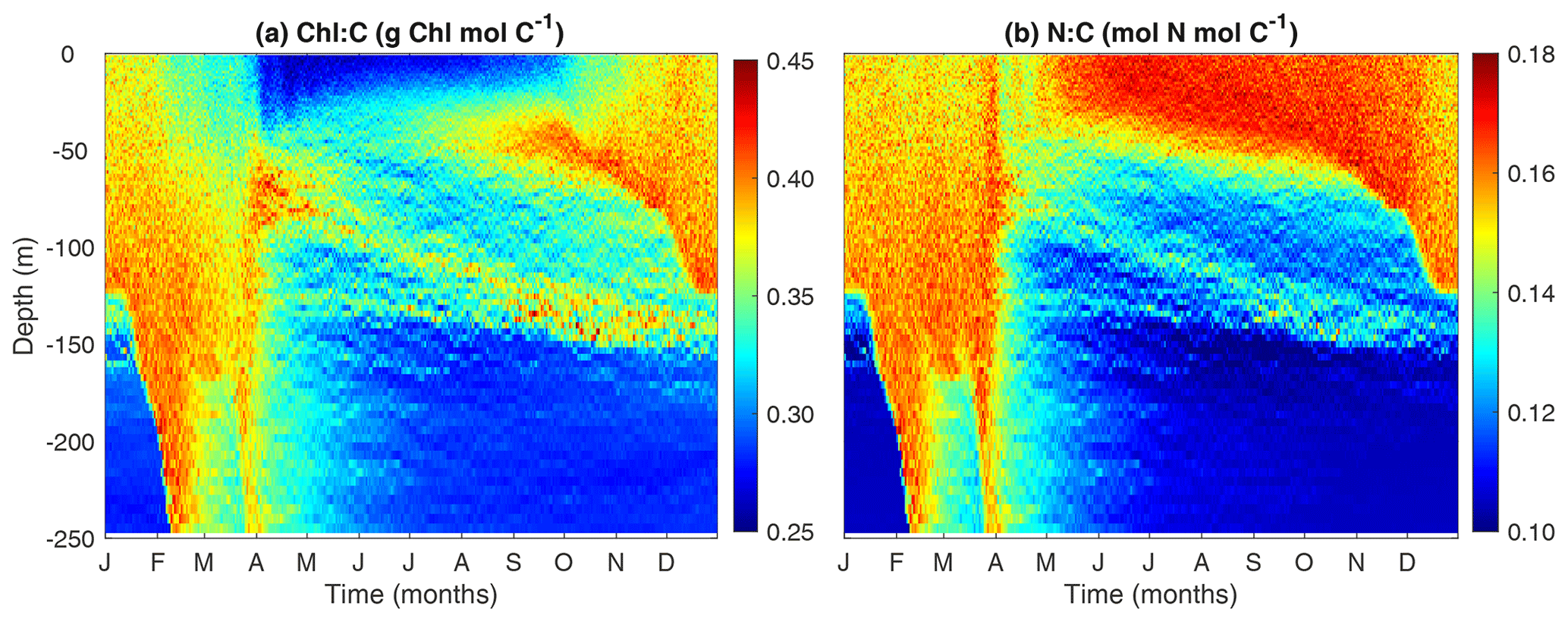
Figure 7 Temporal and vertical variability of modeled phytoplankton (a) Chl:C ratio (g Chl mol C⁻¹) and (b) N:C ratio (mol N mol C⁻¹).

3.6 Modeled phytoplankton trait distribution and functional diversity

Our model reproduces the typical pattern of increasing phytoplankton mean size with nutrient availability (Fig. 8a). Phytoplankton mean size is the smallest at the surface during the summer and autumn, where DIN is low, but increases with depth as nutrients become more abundant. Phytoplankton mean size is also larger at the surface during the winter (but not as large as in deeper waters during summer) when nutrient concentrations are higher due to stronger mixing.

Phytoplankton size variance (Var(C_div)) is an index for size diversity and is the greatest in the area of the deep chlorophyll maximum during summer and autumn and the lowest beneath the euphotic zone (150 m) (Fig. 8b). The high size variance at the deep chlorophyll maximum results from the movements of small cells from above and large cells from below. Size variance is also slightly greater at the surface during the winter than the summer due to more abundant nutrients, but not as high as those in the deep chlorophyll maximum. This suggests that dispersal probably plays the most important role in affecting size diversity.

As expected, phytoplankton community mean T_opt largely follows seawater temperature, with higher values at the surface during summer and lower values at depth (Fig. 8c). However, phytoplankton mean T_opt shows the lowest values at the area of deep chlorophyll maximum during summer and autumn, corresponding to the maximal variance of T_opt (Fig. 8d). Otherwise, the variance of T_opt generally shows larger values in the surface mixed layer than at depth.

Phytoplankton mean light affinity (α^Chl) also follows the opposite pattern of light availability, being the lowest at the summer surface and the highest in the deepest waters (Fig. 8e). The variance of α^Chl shows a qualitatively similar pattern with those of variance of C_div and T_opt, being higher during the winter and at the deep chlorophyll maximum (Fig. 8f), again suggesting mixing can enhance trait variance and diversity. The covariances between traits suggest selection forces against different traits. The covariance between T_opt and C_div is largely negative during the winter, suggesting larger cells tend to be cold-adapted at local scales. Conversely, Cov(T_opt, C_div) is often positive at the surface and the deep chlorophyll maximum during summer at local scales. It is important to note that these covariances are calculated at local scales. We can still observe negative Cov(T_opt, C_div) for the whole water column in which the small and warm-adapted cells are at the surface and large and cold-adapted cells are at depth.

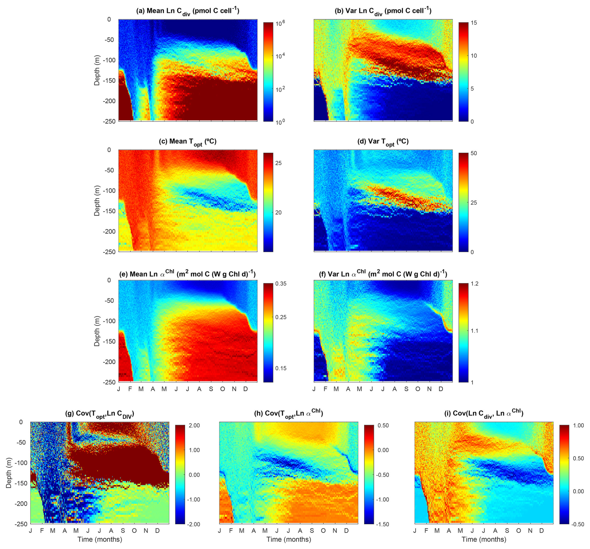
Figure 8 Temporal and vertical variability of modeled phytoplankton traits weighted by phytoplankton carbon content (Eq. 34). (a) Mean phytoplankton size (ESD) back-transformed from the carbon threshold of cell division (C_div). (b) Variance of phytoplankton C_div. (c) Mean phytoplankton optimal temperature (T_opt). (d) Variance of phytoplankton T_opt. (e) Mean phytoplankton light affinity represented by ln-transformed slope of the photosynthesis–irradiance curve (α^Chl). (f) Variance of phytoplankton Ln α^Chl. (g) Covariance between phytoplankton T_opt and Ln C_div. (h) Covariance between phytoplankton T_opt and Ln α^Chl. (i) Covariance between phytoplankton Ln C_div and Ln α^Chl.

The covariance between T_opt and α^Chl is largely negative, suggesting that due to the negative environmental correlation between temperature and light, cold-adapted cells tend to adapt to the low light. The covariance between size and α^Chl is mostly positive during winter and at the deep chlorophyll maximum, indicating larger cells tend to adapt to low light.

The modeled patterns of functional diversity quantified as the Rao index largely follow the trait variances and the covariance between cell size and other two traits (Fig. 9). The Rao index is greater during the winter season with strong mixing and at the layer of the deep chlorophyll maximum.

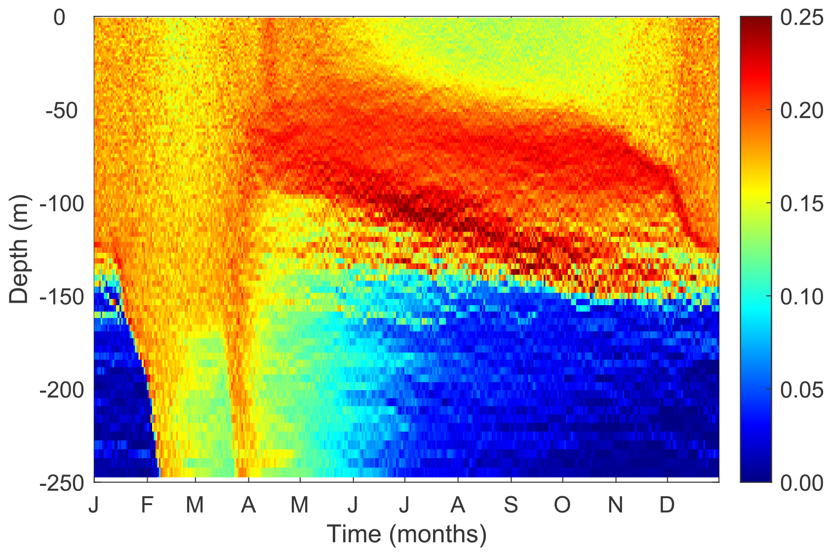
Figure 9 Temporal and vertical variability of phytoplankton functional diversity (Rao index) weighted by cellular carbon.

3.7 Plankton size spectra

During both seasons, log abundances form linear relationships with log size (biovolume) for both phytoplankton and zooplankton (Fig. 10). The slopes of phytoplankton size spectra were between −0.99 and −1.36, consistent with what would be expected for phytoplankton communities in oligotrophic oceans (Marañón, 2019). The slopes of the phytoplankton size spectra were more negative in the summer than in the winter, also consistent with previous observations that the phytoplankton size spectra became steeper and small phytoplankton became more dominant when nutrient supply diminished (Huete-Ortega et al., 2014).

In contrast, the slopes of zooplankton were similar between summer (−0.85) and winter (−0.80) and were less steep than those of phytoplankton. This relates to three factors. First, large zooplankton have a wider feeding kernel than small ones, thus having access to a wide range of prey. Second, the predator-prey size ratio increases with predator size, which makes the slope of size spectra less steep (Trebilco et al., 2013). Third, large zooplankton can also feed on small zooplankton. These patterns are consistent with the observations in marine plankton communities that more biomass can exist in larger size classes, which leads to an inverted biomass pyramid (Gasol et al., 1997; Trebilco et al., 2013).

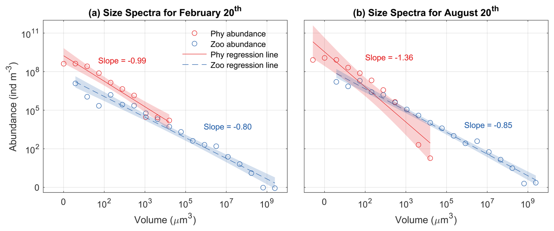
Figure 10 Phytoplankton (Phy) and zooplankton (Zoo) size spectra at the surface during (a) winter (20 February) and (b) summer (20 August). Open dots represent the abundance of each size class, while solid lines indicate the ordinary least squares regression fits. Shaded areas denote the 95 % confidence intervals (α=0.05). The slopes of each regression line are also displayed.

3.8 Diel variability of phytoplankton cell

Our model allows us to track the properties of a phytoplankton cell throughout a diel cycle to gain insights from the life history of the cell. Figure 11 shows the trajectory of a randomly selected super-individual at hourly resolution during the first week of winter and the first week of summer.

During the winter period, this phytoplankton particle was dispersed widely between the surface and 50 m in the water column due to strong mixing (Fig. 11a). Because the water column was well mixed, it was exposed to relatively stable conditions of temperature (∼ 19.50 °C) and DIN (Fig. 11b, d). By contrast, this particle experienced variable PAR conditions, oscillating between daily maximums ∼ 50 and 200 W m⁻². By comparison, the variations of Chl:C ratio (θ^C) are modest (Fig. 11h), suggesting its limited acclimation capability.

During the summer period, the super-individual position was more stable at around 35 m in the first 7 d due to weak mixing (Fig. 11a). As a consequence, the environmental conditions (temperature, DIN, and PAR) the particle experienced were relatively stable. However, the variabilities of phytoplankton N:C and Chl:C are of the same magnitude between summer and winter, mainly due to diel changes of light. The phytoplankton N:C and Chl:C were higher during the winter period (Fig. 11g, red line) than during the summer (blue line), reflecting the higher nutrient and lower light environment in the winter.

Despite the seasonal differences, both particles divided twice during this period (Fig. 11e–f). The phytoplankton cellular carbon content increased progressively with time before the division event until reaching the division threshold (Fig. 11f). When this threshold was reached, the number of phytoplankton cells doubled and the cellular carbon, nitrogen and Chl content halved (Fig. 11e–f).

Irrespective of the birth event, we can also observe clear diel changes in cellular carbon, nitrogen, and chlorophyll contents induced by light-driven photosynthesis, nutrient uptake, chlorophyll synthesis, and dark respiration. Cellular carbon increased from sunrise to sunset but declined in the dark due to respiration. Correspondingly, N:C and Chl:C ratios declined during the daytime and increased during the nighttime.

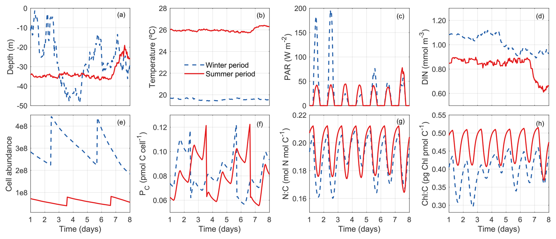
Figure 11 Tracking a randomly selected phytoplankton super-individual for 7 d (hourly resolution) during the winter (blue dashed lines) and the summer (red solid lines) periods. (a) Depths (m) between which the super-individual oscillated in the water column. (b) Differences in the temperature (°C) conditions experienced by the super-individual. (c) Differences in the photosynthetically active radiation conditions (PAR; W m⁻²) experienced by the super-individual. (d) Differences in the nitrogen concentration conditions (NO₃, pmol N m⁻³) experienced by the super-individual. (e) Temporal evolution of phytoplankton cell abundance (number of cells) within the selected super-individual. (f) Temporal evolution of cellular carbon content (P_C, pmol C cell⁻¹). (g) Temporal evolution of nitrogen cellular quota (Q^N, pmol N pmol C⁻¹). (h) Temporal evolution of chlorophyll to carbon cellular ratio (θ^C, mg Chl mmol C⁻¹).

3.9 Effect of the number of super-individuals

We investigated the effect of the number of phytoplankton super-individuals on the key model outputs including DIN, phytoplankton biomass, NPP, and diversity by running four simulations with 5000, 10 000, 20 000, and 50 000 super-individuals. We computed the temporal trends of these variables integrated throughout the water column during the final year of each simulation (Fig. 12).

The number of phytoplankton super-individuals has weak effects on these variables. Increasing the number of super-individuals tends to reduce DIN and increase phytoplankton biomass and NPP, although the trends are very similar between 20 000 and 50 000 super-individuals. Contrary to what one might expect, increasing the number of super-individuals slightly reduces phytoplankton functional diversity, particularly in the winter and summer, although the seasonal trends are qualitatively similar. In summary, the number of phytoplankton super-individuals does not have an appreciable effect on modeled phytoplankton biomass and diversity.

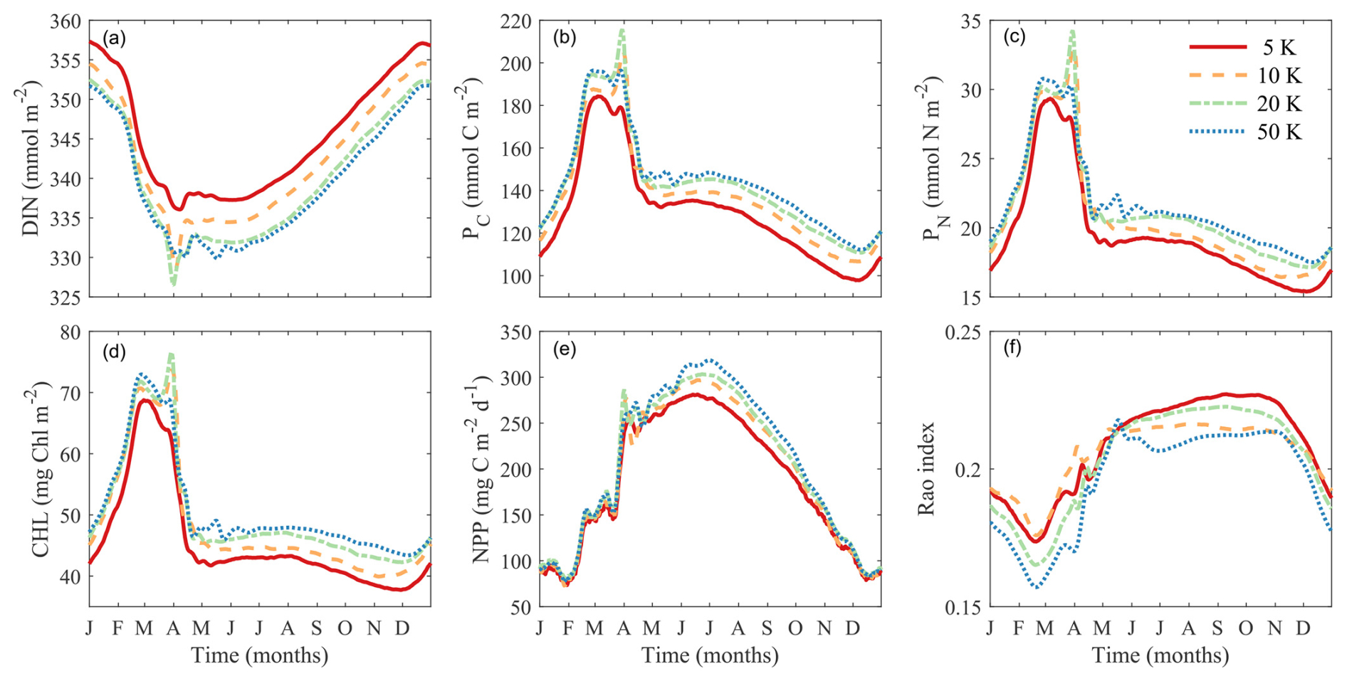
Figure 12 Comparisons of simulations with different numbers of super-individuals on vertically integrated variables. (a) Dissolved inorganic nitrogen (DIN, mmol m⁻²). (b) Phytoplankton carbon (P_C, mmol C m⁻²). (c) Phytoplankton nitrogen (P_N, mmol N m⁻²). (d) Chlorophyll (Chl, mg m⁻²). (e) Net primary production (NPP, mg C m⁻² d⁻¹). (f) Phytoplankton functional diversity (Rao index).

3.10 Comparisons with simple NPZD models

We compared the model outputs of DIN, Chl, and NPP between two simple NPZD models, Eulerian and Lagrangian, and PIBM (Fig. 13). Overall, the three models produce qualitatively similar seasonal and vertical patterns. All three models generate similar concentrations of DIN, although DIN is depleted earlier during spring in PIBM than in the two NPZD models.

The two NPZD models reproduce clear deep chlorophyll maximum (DCM) layers during summer and autumn. In contrast, the DCM in PIBM is broader and less pronounced. One notable difference is that the DCM layers are deeper in the two NPZD models than PIBM. This difference arises from how phytoplankton traits, acclimation, and vertical dynamics are represented in each model. In the NPZD models, phytoplankton traits are fixed and chlorophyll accumulates near the base of the euphotic zone where light and nutrient availability provide an optimal combination for growth. In PIBM, phytoplankton follow individual vertical trajectories and undergo local selection and physiological acclimation. For instance, ecotypes adapted to low-light conditions, with high Chl:C ratios, can persist in the lower layers of the euphotic zone. During summer, when the water column is strongly stratified and vertical movement is constrained, one might expect similar chlorophyll distributions across model frameworks. However, PIBM produces higher chlorophyll concentrations in the upper euphotic zone, as trait selection favor types with elevated growth rates at higher light levels. The shallower DCM in PIBM also results from stronger light attenuation in the upper euphotic zone, where chlorophyll concentrations are elevated. This increases light attenuation and reduces irradiance at depth, limiting the potential for phytoplankton growth and chlorophyll accumulation in deeper layers, as observed in the Eulerian models. While PIBM is the only model that includes photoinhibition, this is offset by the selection of high-light adapted ecotypes under high-light conditions (Fig. 8e).

The two NPZD models also produce higher NPP levels than PIBM, although the seasonal and vertical patterns are qualitatively similar. Notably, the outputs produced by the Lagrangian NPZD model are almost identical to those of the Eulerian NPZD model, although with slightly greater spatiotemporal variation. In summary, the outputs generated by PIBM are broadly consistent with those from the simpler NPZD models, although differences in vertical chlorophyll structure and productivity reflect the influences of traits and acclimation.

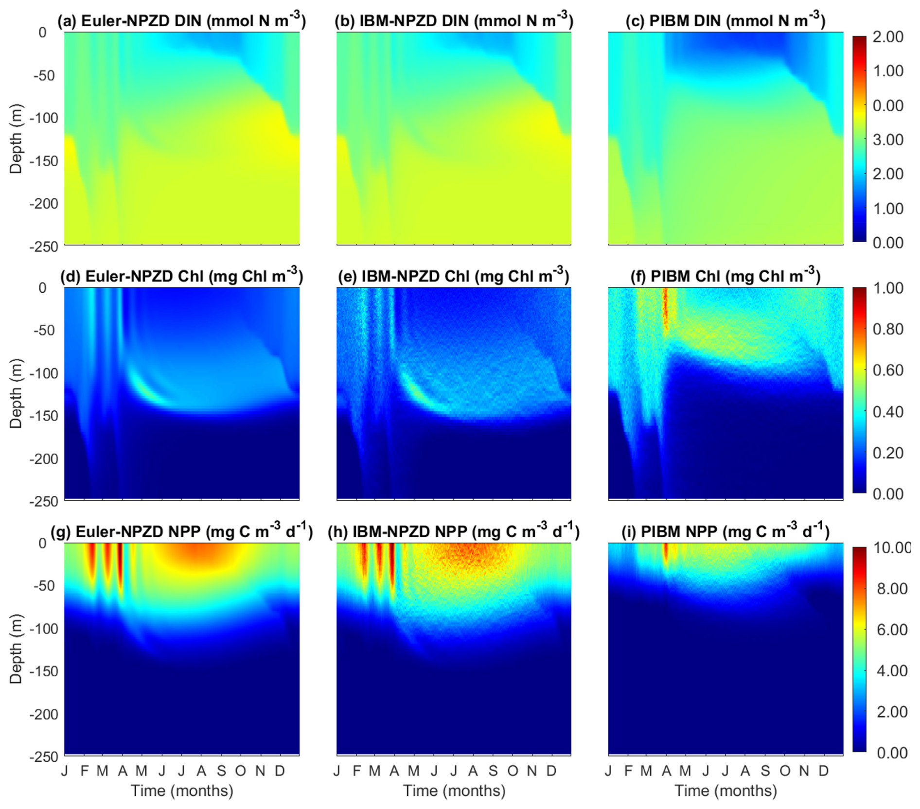
Figure 13 Temporal and vertical variability comparison of the output results of the three models: the Eulerian NPZD model (left column), the Lagrangian NPZD model (middle column), and the PIBM (right column). (a, b, c) Dissolved inorganic nitrogen (DIN, mmol N m⁻³). (d, e, f) Chl a (Chl, mg m⁻³). (g, h, i) Net primary production (NPP, mg C m⁻³ d⁻¹).

4 Discussion

We have presented a novel hybrid Eulerian-Lagrangian plankton model (PIBM) that treats phytoplankton as particles or super-individuals. Each phytoplankton super-individual is associated with three master traits – cell size (C_div), temperature affinity (T_opt), and light affinity (α^Chl) – which govern various physiological traits related to nutrient uptake and photosynthesis. PIBM also enables phytoplankton cells to acclimate and evolve, making it well-suited for addressing many questions in phytoplankton ecology and evolution.

Before discussing the merits and limitations of PIBM, it is important to reiterate that its development was not aimed at improving the modeling of commonly measured bulk variables such as nutrient and chlorophyll concentrations. On the contrary, it is well known that more complex models often provide less accurate predictions of these variables than simpler models (Kwiatkowski et al., 2014), due to greater uncertainties in model structure and parameterization. Indeed, our simple NPZD models can generate outputs as good as, or even better than, PIBM without parameter tuning. However, this does not imply that developing complex models is unnecessary or without value. The same applies to this work, our model is designed as a tool to address research questions related to phytoplankton biodiversity, which simple NPZD models cannot address.

4.1 Model limitations

In this section, we highlight several limitations of PIBM which will be addressed in future work.

A key limitation of PIBM is its high computational cost. This arises from the need for a short time step to accurately simulate the random walk of particles in the water column (Ross and Sharples, 2004). To balance this requirement (<6 s) with computational efficiency, we set the biological reaction time step to 200 times that of the random walk. Additionally, accurately representing the phytoplankton community requires modeling a large number of super-individuals. Since each particle is simulated individually, computational cost scales proportionally with the number of particles. Our sensitivity analyses indicate that 5000 super-individuals appear sufficient to reproduce the main seasonal patterns of phytoplankton diversity and other variables, although some quantitative differences remain (Fig. 12).

We also implemented parallel computing using MPI to simulate the random walk of both passive and phytoplankton particles, with Open MPI as one implementation option. However, the computation is still not fast enough to allow effective sensitivity analysis or parameter optimization. In the future, we will make the computations of biological reactions in parallel and will attempt OpenMP which may allow more efficient memory sharing among threads. Another remedy would be to implement GPU computing to speed up the computation. We are considering ways to integrate our model into PlanktonIndividuals.jl (Wu and Forget, 2022), a Julia language-based phytoplankton individual-based model that can take advantage of GPU computing capability of the Julia language.

The second limitation relates to the inadequate parameterization of the phytoplankton model using laboratory data and the need for more extensive validation of the overall model output. While the size scaling of nutrient uptake has been studied extensively in the literature (e.g., Edwards et al., 2012; Marañón et al., 2013) and the temperature dependence of phytoplankton growth seems clear (Thomas et al., 2012; Chen, 2022), the influence of phytoplankton light traits on growth remains relatively unknown, particularly in the context of photoacclimation. Edwards et al. (2015) analyzed the relationships between light traits (e.g., slope of the photosynthesis-irradiance curve). However, their model did not account for the dependence of photosynthetic rate on the Chl:C ratio or photoinhibition. To account for both the effects of the Chl:C ratio and photoinhibition on phytoplankton photosynthesis, we have to assume an empirical relationship between α^Chl and the repair rate based on differences between high-light adapted and low-light adapted ecotypes of Prochlorococcus (Moore et al., 1998). However, it remains unclear how this scaling relationship applies to phytoplankton in general. More data are needed to establish a more reliable relationship between photosynthetic parameters.

The model outputs of phytoplankton traits also need to be validated against observations. While the measurements of phytoplankton size structure can be obtained, other traits such as T_opt and α^Chl are difficult to measure in situ on a cellular basis. Moreover, even bulk properties such as the N:C and Chl:C ratios of the whole phytoplankton assemblage are challenging to measure in situ due to the difficulties in quantifying phytoplankton carbon and nitrogen. Only a few studies have managed to measure cellular carbon and/or nitrogen of small size phytoplankton using flow cytometric sorting (Graff et al., 2012; Baer et al., 2017). For larger cells, most studies relied on microscopic counting to estimate phytoplankton cell volume which can then be converted to carbon (Cloern, 2018) without any measurement of cellular nitrogen. This type of information is essential for studying biogeochemical cycling and validating ecosystem model outputs.

Another limitation is that the model may be overly complicated if we want to understand the key factor controlling some ecological phenomenon (see below). PIBM considers multiple traits and processes, forming an interconnected feedback network that makes it difficult to isolate the direct effect of a single factor. For example, if we aim to assess whether primary production is limited by nutrient supply or light availability by performing a single-factor perturbation experiment, the increase in nutrient supply will not only affect the nutrient status but also the trait distribution of the whole phytoplankton community. This change in the mean phytoplankton trait depends on the existing trait diversity within the community and the mutation rate of individual cells, both of which remain poorly understood (Acevedo-Trejos et al., 2015; Chen et al., 2019). However, if a user already knows that the system can be simplified (e.g., there is little variability in phytoplankton thermal or light traits), they can modify the initial conditions and the mutation rate to remove the unnecessary trait variance. Thus, one can simplify this model to a single-trait (e.g., size) phytoplankton model if desired.

Finally, needless to say that our model only considers one limiting nutrient – nitrogen – without considering other important elements such as phosphorus or silicate. This omission likely contributes to discrepancies between observations and model outputs at BATS, where phosphorus is the limiting nutrient. It is up to the user to decide whether to add these nutrients to the model depending on the question being asked.

4.2 Model strengths

Our model has several strengths:

First, PIBM simulates the movements and acclimation status of phytoplankton cells with different traits in the ocean and helps address the uncertainty of modeling using Eulerian models and measuring NPP using fixed-depth incubations. It has been widely acknowledged that for both Eulerian models and in situ incubations, the estimates of primary production can be biased, although the extent of this bias is uncertain (Barkmann and Woods, 1996; Ross and Geider, 2009; Baudry et al., 2018). Some differences in bias estimates may stem from the traits of phytoplankton cells. Although our preliminary comparison between the simple Eulerian and Lagrangian models shows no significant differences (Fig. 13), it remains to be tested whether incorporating additional traits will influence the divergence between the two approaches. Notably, most previous individual-based phytoplankton models are similar to our simple Lagrangian NPZD model which does not consider phytoplankton functional diversity (i.e., trait differences among cells). Although developing an Eulerian version of PIBM is beyond the scope of this paper, we can investigate how the estimates of primary production estimates differ between Eulerian and Lagrangian models across different environments (e.g., stratified vs. well-mixed water columns) using a simplified version of PIBM.

Second, PIBM captures three dimensions of phytoplankton traits. We followed the DARWIN model (Follows et al., 2007; Barton et al., 2010; Dutkiewicz et al., 2020) to assign three master traits to phytoplankton, with slight differences. The rationale of designing these three traits is that they are largely orthogonal to each other. In other words, small and large cells have an equal probability of being warm-adapted or cold-adapted and they also have the same probability of being high-light-adapted or low-light-adapted. The impact of trait changes on phytoplankton acclimation and differences in primary production estimates between Eulerian and Lagrangian models remains to be investigated using PIBM.

Third, our phytoplankton model allows phytoplankton evolution. We incorporated phytoplankton evolution into the Lagrangian module, allowing mutation of all three master traits in phytoplankton super-individuals. Modeling phytoplankton evolution has been a hot topic recently (Ward et al., 2019; Beckmann et al., 2019), and individual-based models provide an ideal and straightforward approach to incorporate mutation and evolution (Acevedo-Trejos et al., 2022). We will use PIBM to further investigate the impact of evolution on phytoplankton diversity and primary productivity.

4.3 Potential applications

Below we discuss several potential applications of our model. Note that these are not exhaustive but highlight promising directions for future research.

4.3.1 Validating in situ measurements of primary production

As discussed above, a key application of our model is to assess bias in in situ primary production measurements, where incubation bottles are tethered at fixed depths, exposing phytoplankton to different light conditions than those experienced in a dynamically mixed water column. While several studies have attempted to address this problem using Lagrangian phytoplankton models (Barkmann and Woods, 1996; Baudry et al., 2018; Tomkins et al., 2020), they often overlook phytoplankton traits. The most important phytoplankton trait for this problem are likely light-related traits (e.g., α^Chl), which are rarely considered in Lagrangian phytoplankton models.

In addition, it is not only the trait itself but also the trait distribution that can matter for primary production. In other words, phytoplankton diversity and community composition is essential for accurately assessing in situ primary production measurements. Since phytoplankton trait distribution is not static across time and space, the bias also depends on the phytoplankton community being sampled, so there is no guarantee that the bias can be easily extrapolated to other cases. The caveat is that we need to know the phytoplankton trait distributions (which are even harder to measure) to assess the accuracy of primary production estimates.

4.3.2 Understanding what controls phytoplankton diversity

The central theme of ecology revolves around understanding the factors that regulate biodiversity. Vellend and Agrawal (2010) presented a unified view of four processes controlling biodiversity: selection, dispersal, drift, and evolution. While many studies investigate what regulates phytoplankton diversity in the ocean (Barton et al., 2010; Vallina et al., 2014; Righetti et al., 2019; Dutkiewicz et al., 2020), few managed to examine the holistic effects of all four processes on biodiversity.

PIBM already incorporates the processes of selection, dispersal, and evolution and can be easily adapted to include drift. One challenge would be again about the computational costs if one wishes to understand the large-scale patterns of phytoplankton diversity by coupling the individual-based model with a global circulation model (Hellweger et al., 2014). Nevertheless, this challenge can be addressed using advanced computing techniques as described above.

4.3.3 Understanding how phytoplankton acclimation and trait distribution affect phytoplankton distribution

Biological oceanographers have long been fascinated by distinctive patterns of phytoplankton distribution in the ocean such as the deep chlorophyll maximum (Cullen, 2015) and spring bloom (Behrenfeld, 2010; Lévy, 2015). Despite extensive study, debates persist on what mechanisms drive these patterns.

The formation of deep chlorophyll maximum remains enigmatic with ongoing debate as to whether it reflects an actual accumulation of phytoplankton biomass or is primarily driven by photoacclimation for which phytoplankton cells increase their intracellular pigment content to acclimate to the low light condition. There is evidence that some phytoplankton species may be more abundant at the surface but show a peak of total pigments at the layer of deep chlorophyll maximum, while some other species may indeed show greater biomass at this layer (Chen et al., 2011). Again, the location of the phytoplankton biomass peak likely depends on phytoplankton traits. Our model is an ideal tool for elucidating the contribution of real biomass versus the photoacclimation effect to the layer of deep chlorophyll maximum.

Similar arguments can be raised for the spring bloom. Behrenfeld (2010) argued that contrary to the light effects (i.e., the critical depth hypothesis), the coupling between phytoplankton growth and zooplankton grazing plays a critical role in inducing the spring bloom. Lévy (2015) also used a 1D NPZD model to test different hypotheses and highlighted the importance of physics forcing on the validity of each hypothesis. However, few studies have considered the roles of the changes in phytoplankton traits and photoacclimation in determining the onset of spring bloom. Our model presents an exciting opportunity to fill this knowledge gap.

4.3.4 Understanding diel variations in phytoplankton cell properties

Another potential application of our model is to understand diel variations in cell size, abundance, and the cell cycle of phytoplankton in the oligotrophic ocean (Vaulot et al., 1995; Li et al., 2022). It is an interesting phenomenon that picophytoplankton cells such as Prochlorococcus and Synechococcus tend to show synchronized growth over a diel light/dark cycle. Phytoplankton cells tend to increase the size from sunrise to sunset but divide in late afternoon or evening, thus creating a mismatch between cell carbon production and abundance (Li et al., 2022). However, these diel rhythms can be different for different groups of phytoplankton (Vaulot and Marie, 1999). It is still unclear how these different patterns can be entirely explained by environmental (light, nutrient) variations or at least partly due to endogenous circadian clock (Heath and Spencer, 1985; Hellweger et al., 2020).

As PIBM is driven by a diel light/dark cycle, it can be used to understand what regulates the changes in cell properties linked to the cell cycle. Our model can be further modified to include cell cycles of phytoplankton to understand what controls phytoplankton division (Pascual and Caswell, 1997). Another promising future direction is to include more molecular processes such as gene expression and protein synthesis into the phytoplankton cell cycle, thus allowing us to link molecular studies with phytoplankton traits (Hellweger, 2020; Hellweger et al., 2020).

5 Conclusions

We introduce a novel 1D hybrid Eulerian–Lagrangian model, uniquely tailored to explore how water column dynamics shape phytoplankton dynamics. Phytoplankton are modeled as super-individuals, a Lagrangian particle that represents a cluster of clonal phytoplankton cells that are physiologically identical and share a common history. Each phytoplankton super-individual is characterized by its cell size, temperature affinity and light affinity. Furthermore, these super-individuals possess the capability to mutate, enhancing the model’s capacity to simulate phytoplankton growth, productivity, and diversity within dynamic aquatic environments.

The seasonal variability of temperature, irradiance, and vertical diffusivity at the BATS station enabled us to evaluate the response of our ecological model to environmental changes. By employing three master traits (size, temperature affinity, and light affinity), the individual-based model illustrates the evolution and acclimation of the phytoplankton community to environmental conditions and the competition between different phytoplankton ecotypes. Furthermore, the model allows individual analysis, allowing us to scrutinize how each phytoplankton super-individual responds to the environmental conditions it encounters throughout its life cycle. While the current version has several weaknesses, such as high computational costs and the need for extensive parameterization and validation, it has several potential applications that would help us address questions related to the individual growth of phytoplankton, as well as the productivity and diversity of the phytoplankton community.