Advanced climate model evaluation with ESMValTool v2.11.0 using parallel, out-of-core, and distributed computing

Earth system models (ESMs) allow numerical simulations of the Earth's climate system. Driven by the need to better understand climate change and its impacts, these models have become increasingly sophisticated over time, generating vast amounts of data. To effectively evaluate the complex state-of-the-art ESMs and ensure their reliability, new tools for comprehensive analysis are essential. The open-source community-driven Earth System Model Evaluation Tool (ESMValTool) addresses this critical need by providing a software package for scientists to assess the performance of ESMs using common diagnostics and metrics. In this paper, we describe recent significant improvements of ESMValTool's computational efficiency, which allow a more effective evaluation of these complex ESMs and also high-resolution models. These optimizations include parallel computing (execute multiple computation tasks simultaneously), out-of-core computing (process data larger than available memory), and distributed computing (spread computation tasks across multiple interconnected nodes or machines). When comparing the latest ESMValTool version with a previous not yet optimized version, we find significant performance improvements for many relevant applications running on a single node of a high-performance computing (HPC) system, ranging from 2.3 times faster runs in a multi-model setup up to 23 times faster runs for processing a single high-resolution model. By utilizing distributed computing on two nodes of an HPC system, these speedup factors can be further improved to 3.0 and 44, respectively. Moreover, evaluation runs with the latest version of ESMValTool also require significantly less computational resources than before, which in turn reduces power consumption and thus the overall carbon footprint of ESMValTool runs. For example, the previously mentioned use cases use 2.3 (multi-model evaluation) and 23 (high-resolution model evaluation) times less resources compared to the reference version on one HPC node. Finally, analyses which could previously only be performed on machines with large amounts of memory can now be conducted on much smaller hardware through the use of out-of-core computation. For instance, the high-resolution single-model evaluation use case can now be run with 8 GB of available memory despite an input data size of 35 GB, which was not possible with earlier versions of ESMValTool. This enables running much more complex evaluation tasks on a personal laptop than before.

1 Introduction

Earth system models (ESMs) are crucial for understanding the present-day climate system and for projecting future climate change under different emission pathways. In contrast to early atmosphere-only climate models, modern-day ESMs participating in the latest phase of the Coupled Model Intercomparison Project (CMIP6; Eyring et al., 2016) allow numerical simulations of the complex interactions of the atmosphere, ocean, land surface, cryosphere, and biosphere. Such simulations are essential in assessing details and implications of climate change in the future and are the base for developing effective mitigation and adaptation strategies. For this, thorough evaluation and assessment of the performance of these ESMs with innovative and comprehensive tools are a prerequisite to ensure reliability and fitness for the purpose of their simulations (Eyring et al., 2019).

To facilitate this process, the Earth System Model Evaluation Tool (ESMValTool; Righi et al., 2020; Eyring et al., 2020; Lauer et al., 2020; Weigel et al., 2021; Schlund et al., 2023) has been developed as an open-source, community-driven software. ESMValTool allows for the comparison of model outputs against both observational data and previous model versions, enabling a comprehensive assessment of a model's performance. Through its core functionalities (ESMValCore; see Righi et al., 2020), which are completely written in Python, ESMValTool provides efficient and user-friendly data processing for commonly used tasks such as horizontal and vertical regridding, masking of missing values, extraction of regions/vertical levels, and calculation of statistics across data dimensions and/or data sets, among others. A key feature of ESMValTool is its commitment to transparency and reproducibility of the results. The tool adheres to the FAIR Principles for research software (Findable, Accessible, Interoperable, and Reusable; see Barker et al., 2022) and provides well-documented source code, detailed descriptions of the metrics and algorithms used, and comprehensive documentation of the scientific background of the diagnostics. Users can define their own evaluation workflows with so-called recipes, which are YAML files (https://yaml.org/, last access: 10 December 2024) specifying all input data, processing steps, and scientific diagnostics to be applied. This provides a flexible and customizable approach to model assessment. All output generated by ESMValTool includes a provenance record, meticulously documenting the input data, processing steps, diagnostics applied, and software versions used. This approach ensures that the results are traceable and reproducible. By now, ESMValTool is a well-established and widely used tool in the climate science community used, for instance, to create figures of the Sixth Assessment Report (AR6) of the Intergovernmental Panel on Climate Change (IPCC; e.g., Eyring et al., 2021) and has been selected as one of the evaluation tools listed by the CMIP7 climate model benchmarking task team (see https://wcrp-cmip.org/tools/model-benchmarking-and-evaluation-tools/ and https://wcrp-cmip.org/cmip7/rapid-evaluation-framework/, last access: 10 December 2024).

Since the first major new release of version 2.0.0 in 2020, a particular development focus of ESMValTool has been to improve the computational efficiency of the tool, in particular in the ESMValCore package (Righi et al., 2020), which takes care of the computationally intensive processing tasks. This is crucial for various reasons. First, the continued increase in resolution and complexity of the CMIP models over many generations has led to higher and higher data volumes, with the published CMIP6 output reaching approximately 20 PB (Petrie et al., 2021). Future CMIP generations are expected to provide even higher amounts of data. Thus, fast and memory-efficient evaluation tools are essential for an effective and timely assessment of current and future CMIP ensembles. Second, minimizing the usage of computational resources reduces energy demand and the carbon footprint of HPC and data centers, which are expected to have a steadily increasing contribution to the total global energy demand in the upcoming years (Jones, 2018). Having said this, it should be noted that producing the actual ESM simulations requires much more computational resources than their evaluation with tools like ESMValTool. Finally, faster and more memory-efficient model evaluation reduces the need to use HPC systems for model evaluation and allows using smaller local machines instead. This is especially relevant to the Global South, which still suffers from limited access to HPC resources but at the same time is highly affected by climate change (Ngcamu, 2023).

In this study, we describe the optimized computational efficiency of ESMValCore and ESMValTool available in the latest release, v2.11.0 from July 2024. Note that these improvements were not implemented within one release cycle but rather developed in a continuous effort over the last years. The three main concepts we have used here are (1) parallel computing (i.e., performing multiple computation tasks simultaneously rather than sequentially), (2) out-of-core computing (i.e., processing data that are too large to fit into available memory), and (3) distributed computing (i.e., spreading computational tasks across multiple interconnected nodes or machines). We achieve this by consequently making use of state-of-the-art computational Python libraries such as Iris (Iris contributors, 2024) and Dask (Rocklin, 2015).

This paper is structured as follows: Sect. 2 provides a technical description of the improvements in computational efficiency in the ESMValCore and ESMValTool packages. Section 3 presents example use cases to showcase the performance gain through these improvements, which are then discussed in Sect. 4. The paper closes with a summary and outlook in Sect. 5.

2 Improving computational efficiency

The main strategy for improving the computational efficiency in our evaluation workflow is by consistently using Dask (Rocklin, 2015), a powerful Python package designed to speed up computationally intensive tasks for array computations. An overview of Dask can be found in its documentation, for example in the form of a clear and concise 10 min introduction (https://docs.dask.org/en/stable/10-minutes-to-dask.html, last access: 10 December 2024), which we summarize in the following.

Dask breaks down computations into individual tasks. Each task consists of an operation (e.g., compute maximum) and corresponding arguments to that operation (e.g., input data or results from other tasks). A key concept here is the partitioning of the involved data into smaller chunks that fit comfortably into the available memory, which enables Dask to also process data that are too large to fit entirely into memory (out-of-core computing). A Dask computation is represented as a task graph, which is a directed acyclic graph (DAG) where each node corresponds to a task and each edge to the dependencies between these tasks. This task-based approach allows Dask to effectively parallelize computations (parallel computing) and even distribute tasks across multiple interconnected machines like different nodes of an HPC system (distributed computing). The task graph is then executed by the so-called scheduler, which orchestrates the tasks, distributes them efficiently across available workers (components that are responsible for running individual tasks), and monitors their progress.

In practice, this may look as follows: first, the input data are loaded lazily (i.e., only metadata like the arrays' shape, chunk size, and data type are loaded into memory; the actual data remain on disk). Then, the task graph is built by using Dask structures and functions, for example, dask.array objects instead of numpy (Harris et al., 2020) objects. Again, this will not load any data into memory but merely sets up the tasks. Typically, the task graph consists of operations which only operate on single chunks and operations which aggregate the results from these “chunked” operations. For example, to calculate the maximum of an array, an approach is to first calculate the maxima over the individual chunks and then calculate the maximum across the individual maxima. Finally, these tasks will be executed by the workers as directed by the scheduler, which will eventually load the actual data into memory in small chunks and perform all desired computations defined in the task graph.

Dask offers different scheduler types, and choosing the most appropriate one for a specific application is crucial for optimum performance. By default, Dask uses a simple and lightweight single-machine scheduler, which is, for array-based workflows like our use cases here, based on threads. One major drawback of this scheduler is that it can only be used on a single machine and does not scale well. A powerful alternative is the Dask distributed scheduler, which, despite having the word “distributed” in its name, can also be used on a single machine. This scheduler is more sophisticated, allows distributed computing, and offers more features like an asynchronous application programming interface (API) and a diagnostic dashboard, but it adds slightly more overhead to the tasks than the default scheduler and also requires more knowledge to configure correctly.

Whenever possible, we do not use Dask directly but rely on the Iris package (Iris contributors, 2024) for data handling instead. Iris is a Python package for analyzing and visualizing Earth science data. In the context of ESMValTool, a key feature of Iris is the built-in support for data complying with the widely used climate and forecast (CF) conventions (https://cfconventions.org/, last access: 10 December 2024), which all input data of ESMValTool are expected to follow (see Schlund et al., 2023, for details on this). Iris provides a high-level interface to Dask; for example, iris.load() will load data lazily, or iris.save() will execute the Dask task graph and save the resulting output to disk.

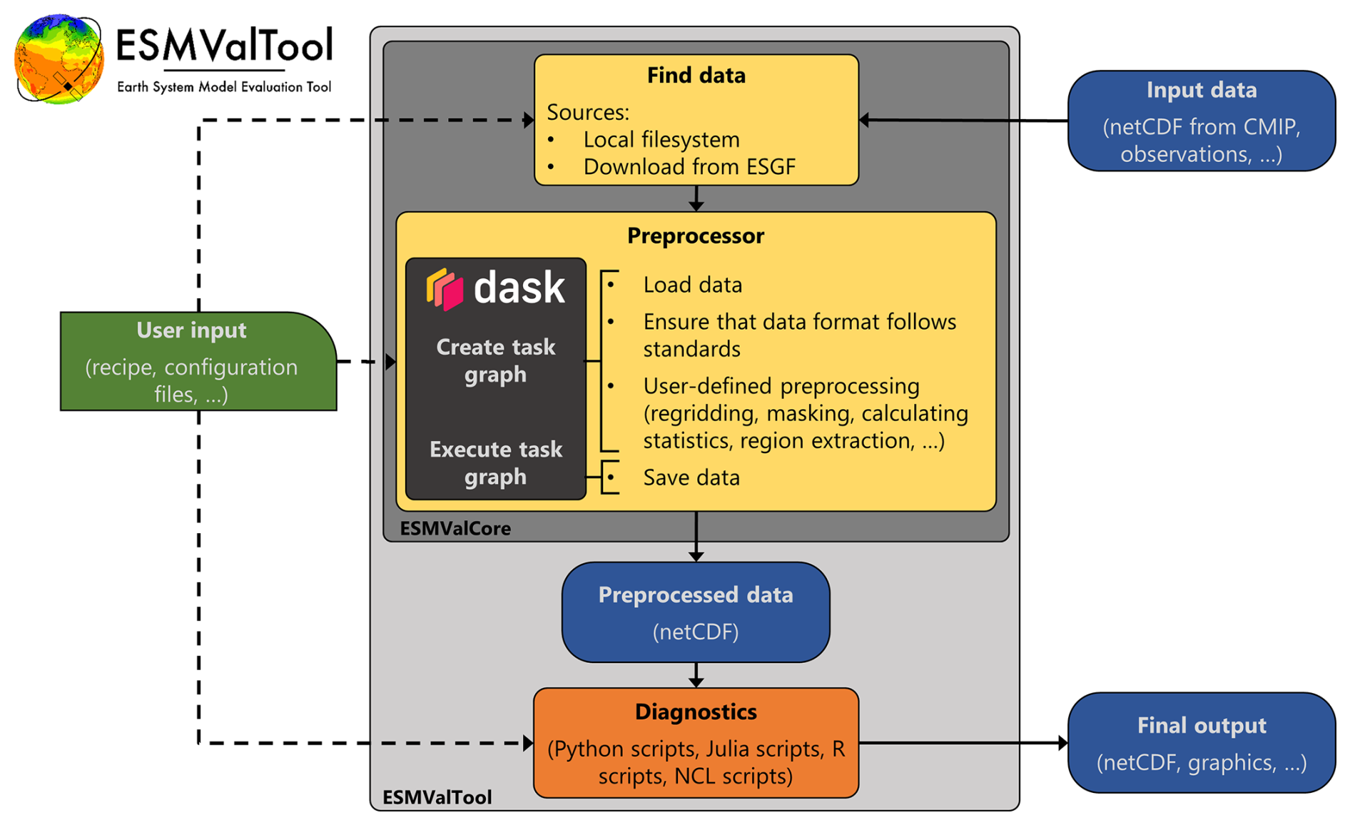
Figure 1 Schematic representation of ESMValTool (light-gray box). Input data are located and processed by the ESMValCore package (dark-gray box), which is a dependency of ESMValTool. The preprocessed data written by ESMValCore are then used as input by the scientific diagnostic scripts, which typically produce the final output of ESMValTool. User input is given via YAML files like the recipe and configuration files (green box). Since ESMValCore's preprocessor performs the majority of the computationally intensive operations, enhancing its computational efficiency with Dask yields the highest overall performance improvements for ESMValTool.

Figure 1 provides a schematic overview of the usage of Dask in ESMValTool v2.11.0. To determine the relative runtime contributions of the individual components, we used the py-spy sampling profiler (https://github.com/benfred/py-spy, last access: 10 December 2024). The computationally most intensive part is the preprocessor, which is part of ESMValCore (dark-gray box in the figure), a dependency of ESMValTool that contains all of the tool's core functionalities, including all data preprocessing functions. Thus, enhancing the computational efficiency of ESMValCore's preprocessor through the use of Dask yields the most significant overall performance improvements. In practice, this is achieved as follows: the data are lazily loaded via Iris. After that, the individual preprocessor steps are executed (mandatory ones like data validation as well as the custom ones like regridding and masking, among others), which will build up the Dask task graph. This is done by using Dask or available corresponding Iris functionalities wherever possible but oftentimes also requires custom code. For example, when regridding data to a higher resolution, the regridding preprocessor function needs to resize the input chunks before regridding so the output chunk sizes fit into memory. Similarly, the multi-model statistics preprocessor function requires that all data share the same calendar. Finally, a call to iris.save() loads the data into memory (in small chunks), executes the task graph, and saves the preprocessor output to disk. Implementing this pipeline in a computationally efficient way has been a massive effort over the last years and is still ongoing. For example, as of 10 December 2024, 95 pull requests mention the key words “dask” or “performance” in the ESMValCore repository. The Dask workflow within ESMValTool is highly customizable via configuration files (see Appendices A and B), which allows selecting the type of scheduler, the number of workers, the amount of memory used, etc. The Dask configuration needs to be adapted to the actual use case, i.e., the corresponding evaluation task and the available hardware (memory, CPUs, etc.). Dask can also be used to improve the efficiency of scientific Python diagnostics in ESMValTool (see orange box in Fig. 1); however, since the bulk of the computationally intensive work is usually performed by the preprocessor, this only improves overall performance significantly in a few selected cases where heavy computations are also done within a diagnostic. One major improvement in recent versions of ESMValTool, ESMValCore, and Iris is the added support for Dask distributed schedulers. As stated above, this scheduler type enables distributed computing but can also provide substantial performance boosts on single-machine setups. Before introducing these changes, only the default thread-based scheduler could be used.

3 Use cases

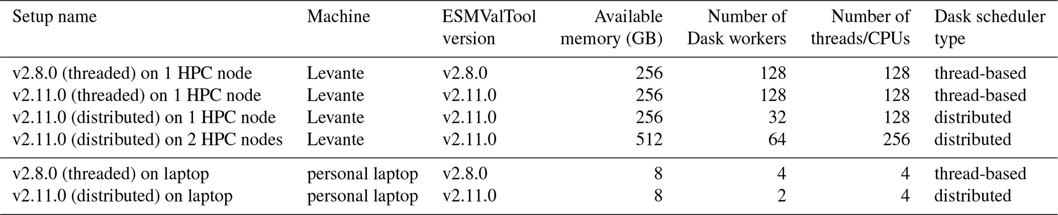
To showcase the improved computational efficiency of ESMValTool v2.11.0, this section provides examples of real-world use cases. The analyses we perform here measure the performance of ESMValTool along two dimensions: (1) different versions of ESMValTool and (2) different hardware setups. For (1), we compare the latest ESMValTool version 2.11.0 (with ESMValCore v2.11.1, Iris v3.11.0, and Dask v2025.2.0) against the reference version 2.8.0 (with ESMValCore v2.8.0, Iris v3.5.0, and Dask v2023.4.1), which is the last version of ESMValTool with no support of Dask distributed schedulers. Using older versions than v2.8.0 as a reference would yield even larger computational improvements. For (2), we compare running ESMValTool on different hardware setups using two different machines: (a) the state-of-the-art BullSequana XH2000 supercomputer Levante operated by the Deutsches Klimarechenzentrum (DKRZ) (see https://docs.dkrz.de/doc/levante/, last access: 10 December 2024) and (b) a Dell Latitude 7430 personal laptop with a 12th-generation Intel(R) Core(TM) i7-1270P CPU and 16 GB of memory. An overview of all setups can be found in Table 1. The HPC system (a) allows us to easily vary the number of HPC nodes, CPUs, and amount of memory available, so it can be used to analyze ESMValTool's new parallel and distributed computing capabilities. On the other hand, the personal laptop (b) with its reduced amount of memory is well suited to demonstrate the out-of-core computing capabilities of ESMValTool. When using local hardware, the memory usage of the operating system has to be accounted for; thus, only 8 GB of the available 16 GB of memory is used for the laptop setups.

Table 1 Overview of the different setups used to showcase the improved computational efficiency of ESMValTool v2.11.0.

To analyze computational performance and scalability, we consider ESMValTool runs performed on the HPC system since their different runtimes are directly comparable to each other due to the usage of the exact same CPU type (only the number of cores used varies) and memory per thread/CPU (2 GB). We focus on metrics that measure the relative performance of a system compared to a reference, which allows us to easily transfer our results to other machines than DKRZ's Levante. In this study, the reference setup is the old ESMValTool version v2.8.0 (threaded) run on one HPC node. As main metric of computational performance, we use the speedup factor s. The speedup factor of a new setup relative to the reference setup REF can be derived from the corresponding execution times t and t_REF necessary to process the same problem:

$$\begin{array}{}\text{(1)}& s={\displaystyle \frac{t_{\mathrm{REF}}}{t}}.\end{array}$$

Values of s>1 correspond to a speedup relative to the reference setup and values of s<1 to a slowdown. For example, a speedup factor of s=2 means that a run finishes twice as fast in the new setup compared to the reference setup.

A further metric we use is the scaling efficiency e, which is calculated as the resource usage (measured in node hours) in the reference setup divided by the resource usage in the new setup:

$$\begin{array}{}\text{(2)}& e={\displaystyle \frac{n_{\mathrm{REF}}\cdot t_{\mathrm{REF}}}{n\cdot t}}=s\cdot {\displaystyle \frac{n_{\mathrm{REF}}}{n}}.\end{array}$$

Here, n and n_REF are the number of nodes used in the new and reference setup, respectively. Values of e>1 indicate that the new setup uses less computational resources than the reference setup, and values of e<1 indicate that the new setup uses more resources than the reference setup. For example, a scaling efficiency of e=2 means that using the new setup only uses half of the computational resources (here, node hours) than the reference setup.

We deliberately ignore memory usage here since one aim of using Dask is to rather optimize memory usage instead of simply minimizing it, i.e., to use as much memory as possible (constrained by the system's availability and/or the user's configuration of Dask). A low memory usage is not necessarily desirable but could be the result of a non-optimal configuration. For example, using a Dask configuration file designed for a personal laptop with 16 GB of memory (see, e.g., Appendix A) would be very inefficient and result in higher runtimes on HPC system nodes with 256 GB of memory, since at most 6.25 % of the available memory would be used. Nevertheless, if low memory usage is crucial (e.g., on systems with limited memory), Dask distributed schedulers can be configured to take into account such restrictions, which enables processing of data that are too large to fit into memory (out-of-core computing). Without this feature, processing large data sets on small machines would not be possible.

3.1 Multi-model analysis

The first example illustrates a typical use case of ESMValTool: the evaluation of a large ensemble of CMIP6 models. Here, we focus on the time series from 1850–2100 of the global mean sea surface temperature (SST) anomalies in the shared socioeconomic pathways SSP1-2.6 and SSP5-8.5 from a total of 238 ensemble members of CMIP6 models (O'Neill et al., 2016), as shown in Fig. 9.3a of the IPCC's AR6 (Fox-Kemper et al., 2021). We reproduce this plot with ESMValTool in Fig. 2. As illustrated by the shaded area (corresponding to the 17 %–83 % model range), the models agree well over the historical period (1850–2014) but show larger differences for the projected future time period (2015–2100). A further source of uncertainty is the emission uncertainty (related to the unknown future development of human society), which is represented by the diverging blue and red lines, corresponding to the SSP1-2.6 and SSP5-8.5 scenarios, respectively. SSP1-2.6 is a sustainable low-emission scenario with a relatively small SST increase over the 21st century, while SSP5-8.5 is a fossil-fuel-intensive high-emission scenario with very high SSTs in 2100. For details, we refer to Fox-Kemper et al. (2021).

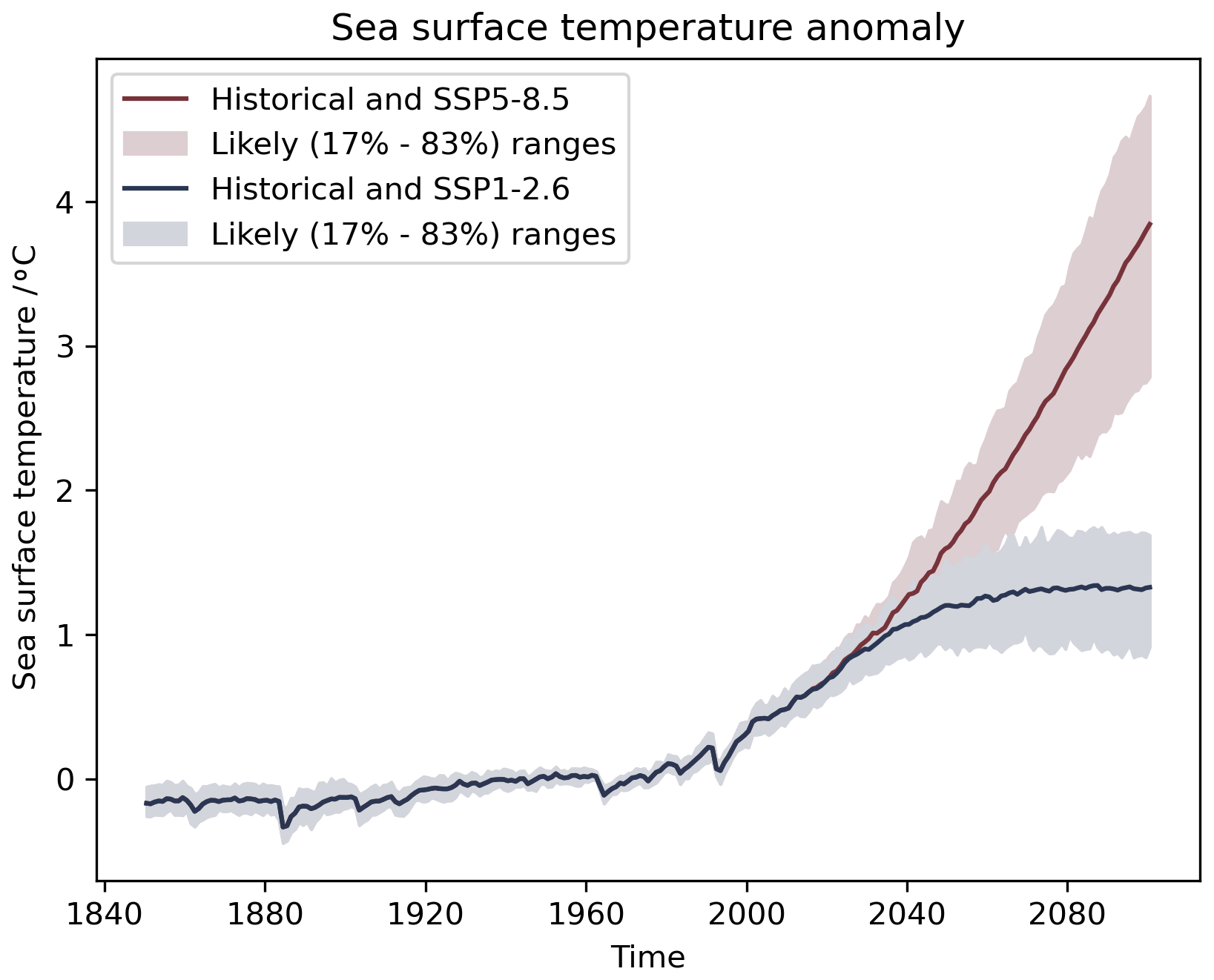
Figure 2 Time series of global and annual mean sea surface temperature anomalies in the shared socioeconomic pathways SSP1-2.6 and SSP5-8.5 relative to the 1950–1980 climatology, calculated from 238 ensemble members of CMIP6 models. The solid lines show the multi-model mean; the shading shows the likely (17 %–83 %) ranges. Similar to Fig. 9.3a of the IPCC's AR6 (Fox-Kemper et al., 2021).

The input data of Fig. 2 are three-dimensional SST fields (time, latitude, longitude) from 238 ensemble members of 33 different CMIP6 models scattered over 3708 files, adding up to around 230 GB of data in total. The following preprocessors are used in the corresponding ESMValTool recipe (in this order):

1. anomalies – calculate anomalies relative to the 1950–1980 climatology;

2. area_statistics – calculate global means;

3. annual_statistics – calculate annual means;

4. ensemble_statistics – calculate ensemble means for the models that provide multiple ensemble members;

5. multi_model_statistics – calculate multi-model mean and percentiles (17 % and 83 %) from the ensemble means.

Table 2 shows the speedup factors and scaling efficiencies of ESMValTool runs to produce Fig. 2 in different HPC setups. Each entry here has been averaged over two independent ESMValTool runs to minimize the effects of random runtime fluctuations. Since the runtime differences within a setup are much smaller than the differences between different setups, we are confident that our results are robust. Version 2.11.0 of ESMValTool on one HPC node performs much better than the reference setup (version 2.8.0 on one HPC node) with a speedup factor of 2.3 (i.e., reducing the runtime by more than 56 %). The scaling efficiency of 2.3 indicates that the recipe can be run 2.3 times as often in the new setup than in the reference setup for the same computational cost (in other words, the required computational costs to run the recipe once are reduced by more than 56 %). By utilizing distributed computing with two HPC nodes, the speedup factor for v2.11.0 further increases to 3.0, but the scaling efficiency drops to 1.5.

Table 2 Speedup factors (see Eq. 1) and scaling efficiencies (see Eq. 2) of ESMValTool runs producing Fig. 2 using different setups (averaged over two ESMValTool runs). Values in bold font correspond to the largest improvements. The speedup factors s and scaling efficiencies e are calculated relative to the reference setup, which requires a runtime of approximately 3 h and 27 min.

3.2 High-resolution data

A further common use case of ESMValTool is the analysis of high-resolution data. Here, we process 10 years of daily near-surface air temperature data (time, latitude, longitude) from a single ensemble member of the CMIP6 model NICAM16-9S (Kodama et al., 2021) with an approximate horizontal resolution of 0.14° × 0.14°. We use results from the highresSST-present experiment (Haarsma et al., 2016), which is an atmosphere-only simulation of the recent past (1950–2014) with all natural and anthropogenic forcings, and SSTs and sea-ice concentrations prescribed from HadISST (Rayner et al., 2003). In total, this corresponds to 35 GB of input data scattered over 11 files. In our example recipe, which is illustrated in Fig. 3, we calculate monthly climatologies averaged over the time period 1950–1960 of the near-surface air temperature over land grid cells for three different regions: Northern Hemisphere (NH) extratropics (30–90° N), tropics (30° N–30° S), and Southern Hemisphere (SH) extratropics (30–90° S). The land-only near-surface air temperature shows a strong seasonal cycle in the extratropical regions (with the NH extratropical temperature peaking in July and the SH extratropical temperature peaking in January) but only very little seasonal variation in the tropics. NH land temperatures are on average higher than SH land temperatures due to the different distribution of land masses in the hemispheres (for example, the South Pole is located on the large land mass of Antarctica (included in the calculation), whereas the North Pole is located over the ocean (excluded from the calculation)).

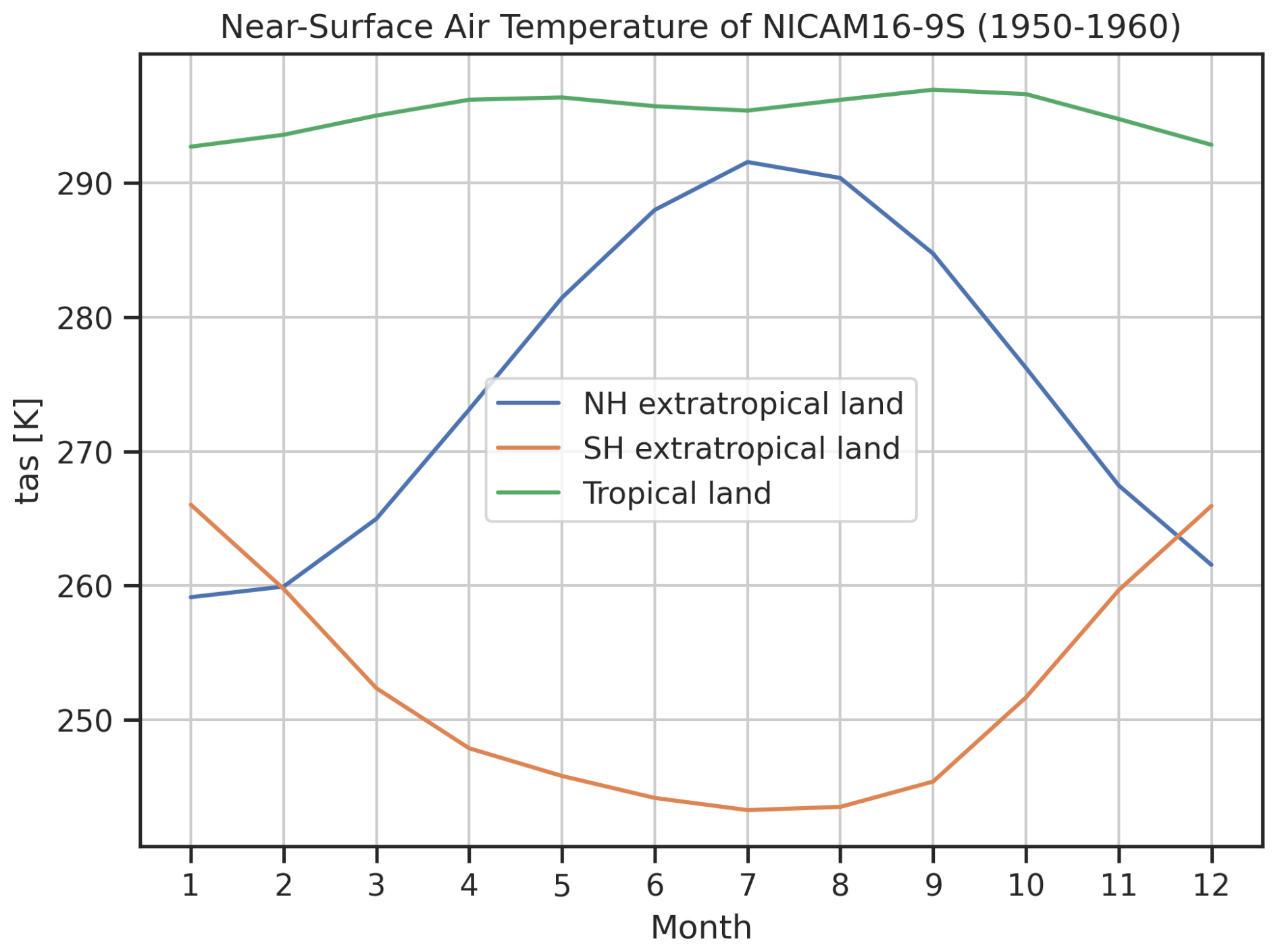
Figure 3 Monthly climatologies of near-surface air temperature (land grid cells only, averaged over the time period 1950–1960) for different geographical regions as simulated by the CMIP6 model NICAM16-9S using the highresSST-present experiment. The regions are defined as follows: Northern Hemisphere (NH) extratropics, 30–90° N; tropics, 30° N–30° S; and Southern Hemisphere (SH) extratropics, 30–90° S.

The ESMValTool recipe to produce Fig. 3 uses the following preprocessors (in this order):

1. mask_landsea – mask out ocean grid cells so only land remains;

2. extract_region – cut out the desired regions (NH extratropics, tropics, and SH extratropics);

3. area_statistics – calculate area mean over the corresponding regions;

4. monthly_statistics – calculate monthly means from daily input fields;

5. climate_statistics – calculate the monthly climatology.

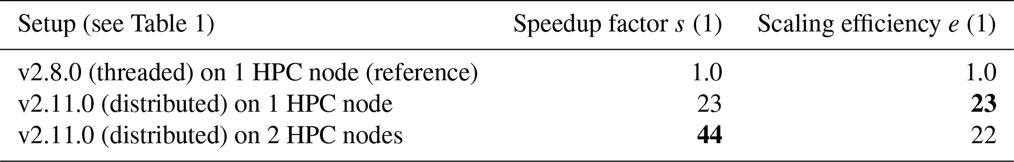
The corresponding speedup factors and scaling efficiencies for running this ESMValTool recipe with different HPC setups are listed in Table 3. Similar to Table 2, the values are averaged over two ESMValTool runs of the same recipe. The runtime differences within setups are again much smaller than the differences between different setups, indicating that the results are robust. Once more, ESMValTool version 2.11.0 performs much better than its predecessor version 2.8.0. We find a massive speedup factor and scaling efficiency of 23 when using ESMValTool v2.11.0 on one HPC node compared to the reference setup (v2.8.0 on one HPC node). When using two entire nodes, the speedup factor further increases to 44, with a slight drop in the scaling efficiency to 22. This demonstrates the powerful distributed computing capabilities of ESMValTool v2.11.0.

Table 3 Speedup factors (see Eq. 1) and scaling efficiencies (see Eq. 2) of ESMValTool runs producing Fig. 3 using different setups (averaged over two ESMValTool runs). Values in bold font correspond to the largest improvements. The speedup factors s and scaling efficiencies e are calculated relative to the reference setup, which requires a runtime of approximately 40 min.

In addition to the HPC system, this evaluation has also been performed on a personal laptop (see two bottom setups in Table 1). Running the recipe fails with ESMValTool v2.8.0 due to insufficient memory since the 35 GB of input data cannot be loaded into the 8 GB of available memory. On the other hand, with ESMValTool v2.11.0 and its advanced out-of-core computing abilities, the recipe finishes in less than 30 min. This runtime cannot be meaningfully compared to the runtimes achieved with the HPC system since the two machines use different CPUs.

3.3 Commonly used preprocessing operations

In this section, the performance of individual preprocessing operations in an idealized setup is shown. For this, the following five preprocessors are applied to monthly-mean, vertically resolved air temperature data (time, pressure level, latitude, longitude) of 20 years of historical simulations (1995–2014) from 10 different CMIP6 models: (1) area_statistics (calculates global area means), (2) climate_statistics (calculates climatologies), (3) regrid (regrids the input data to a regular 5° × 5° grid), (4) amplitude (calculates seasonal cycle amplitudes), and (5) extract_levels (interpolates the data to the pressure levels 950, 850, 750, 500, and 300 hPa). These five preprocessors have been chosen since they are among the most commonly used preprocessors across all available recipes (currently, more than 60 different preprocessors are available in ESMValTool). Figure 4 shows the speedup factors and scaling efficiencies of these preprocessors. In contrast to the previous two sections, this considers the times to run these preprocessors, not the entire runtimes of the corresponding ESMValTool recipes, which can be considerably larger due to computational overhead like searching for input data and data checks, among others.

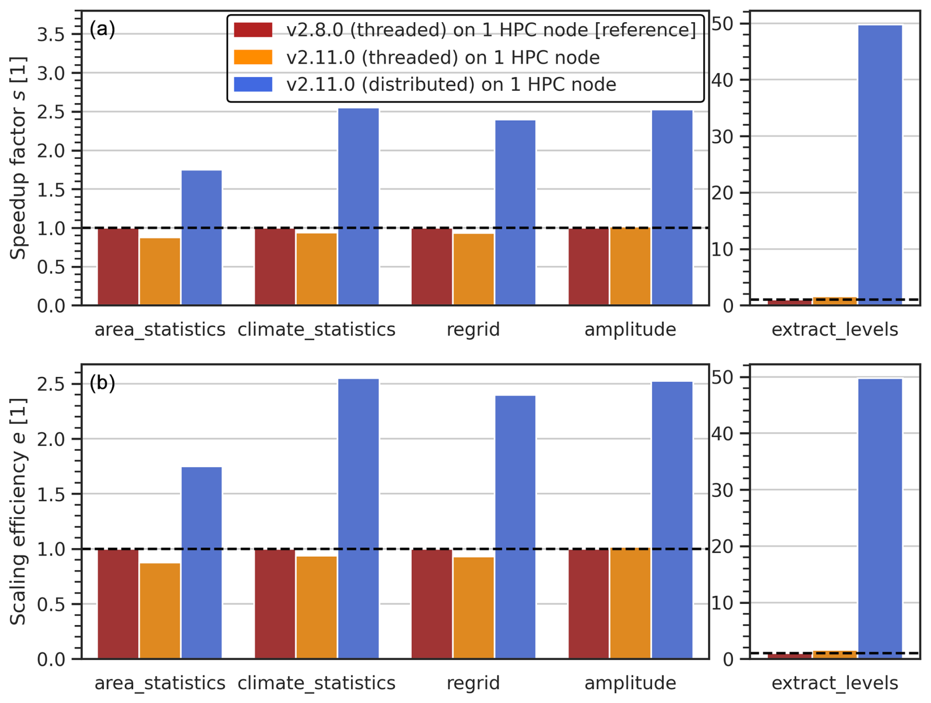
Figure 4 (a) Speedup factors (see Eq. 1) and (b) scaling efficiencies (see Eq. 2) of individual preprocessor runs in different setups (see legend). The speedup factors s and scaling efficiencies e are calculated relative to the reference setup. The input data are monthly-mean vertically resolved air temperature (time, pressure level, latitude, longitude) for 20 years of historical simulations (1995–2014) from 10 different CMIP6 models. The dashed black lines indicate no improvement relative to the reference setup, and values above/below these lines correspond to better/worse performance.

As shown in Fig. 4a, ESMValTool version 2.11.0 with a distributed scheduler consistently outperforms its predecessor version 2.8.0 with the thread-based scheduler on one HPC node. The speedup factors range, depending on the preprocessor, from 1.7 for area_statistics to 50 for extract_levels. For all analyzed preprocessors except extract_levels, using the default thread-based scheduler in v2.11.0 gives speedup factors of ≈ 1, which indicates similar runtimes to v2.8.0. For extract_levels, we find a speedup factor of 1.6 in this setup. Since all analyzed setups use one HPC node, the scaling efficiencies are identical to the speedup factors (see Eq. 2), indicating that ESMValTool v2.11.0 requires less computational resources to run the corresponding preprocessors than v2.8.0 (see Fig. 4b).

4 Discussion

The results above show that ESMValTool's performance is considerably improved in v2.11.0 compared to v2.8.0 through the consistent use of Dask within ESMValTool's core packages, i.e., ESMValCore and Iris.

For the multi-model analysis presented in Sect. 3.1, we find speedup factors and scaling efficiencies of $s=e=\mathrm{2.3}$ on one HPC node and s=3.0 and e=1.5 on two HPC nodes (see Table 2). A major reason for this improvement is the consistent usage of Dask in the preprocessor function multi_model_statistics. For the other real-world example use case shown in Sect. 3.2 (evaluation of a single high-resolution model), even larger performance improvements are found (see Table 3): ESMValTool v2.11.0 on one HPC node is 23 times faster and 23 times more efficient (in terms of computational resources) than ESMValTool v2.8.0. With distributed computing using two HPC nodes, the speedup factor rises to s=44. Since this increase in the speedup factor is smaller than the theoretical limit possible by the higher resource usage, the scaling efficiency drops to e=22. The main reason for these improvements here between ESMValTool v2.8.0 and v2.11.0 is the optimization of the preprocessor mask_landsea with Dask functionalities.

The high-resolution analysis achieves significant performance gains because it uses data from only a single ensemble member of one climate model loaded from just 11 files. Consequently, most of the runtime of this workflow is spent on preprocessing calculations on the array representing near-surface air temperature – a task that can be highly optimized using Dask. In other words, the proportion of operations that can be parallelized is high, leading to a large maximum possible speedup factor (Amdahl's law). For example, if 90 % of the code can be parallelized, the maximum possible speedup factor is 10 since $\mathrm{1}/\mathrm{10}$ of the code cannot be sped up. On the other hand, the multi-model analysis involves a large number of data sets and files (here, data from 238 ensemble members of 33 different CMIP6 models scattered over 3708 files), which require a high number of serial metadata computations like loading the list of available variables in files and processing coordinate arrays (e.g., time, latitude, longitude), resulting in a much larger proportion of serial operations. Consequently, the maximum possible speedup factor and thus the actual speedup factor is a lot smaller in this example. Parallelizing these metadata operations is more challenging because it requires performing operations on Iris cubes (i.e., the fundamental Iris objects representing multi-dimensional data with metadata) on the Dask workers instead of just replacing Numpy arrays with Dask arrays. First attempts at this were not successful due to issues with the ability of underlying libraries (Iris and ESMPy) to run on Dask workers, but we aim to address those problems in future releases. A further aspect that may negatively influence computational performance when loading coordinate data is the Lustre file system used by DKRZ's HPC system Levante, which is not optimized for reading small amounts of data from many files. Moreover, climate model data are usually available in netCDF/HDF5 format, with data written by the climate models typically at each output time step. This can result in netCDF chunk sizes that are far from optimal for reading. For example, reading a compressed time coordinate containing 60 000 points with a netCDF chunk size of 1 (total uncompressed size 0.5 MB) as used for ∼ 20 years of 3-hourly model output can take up to 15 s on Levante.

Amdahl's law also provides a theoretical explanation of why the scaling efficiencies decrease when the number of HPC nodes is increased (see Tables 2 and 3). Due to the serial part of the code that cannot be parallelized, the speedup factor s will always grow slower than the number of HPC nodes n, resulting in a decrease in the scaling efficiencies e with rising n (see Eq. 2). In the limit of infinite nodes n→∞, s approaches a finite value (the aforementioned maximum possible speedup factor); thus, e→0.

Further improvements can be found in ESMValTool's out-of-core computation capabilities. As demonstrated in Sect. 3.2, ESMValTool v2.11.0 allows running the high-resolution model evaluation example on a personal laptop with only 8 GB of memory available, despite an input data size of 35 GB. This is enabled through the consequent usage of Dask, which partitions the input data into smaller chunks that fit comfortable into memory. All relevant computations are then executed on these chunks instead of loading the entire data into memory at once. With the reference version 2.8.0, the corresponding recipe fails to run due to out-of-memory errors.

The analysis of individual preprocessor functions in Sect. 3.3 shows medium improvements for preprocessing operations that were already using Dask in ESMValTool v2.8.0. These include the preprocessor functions area_statistics ($s=e=\mathrm{1.7}$), climate_statistics ($s=e=\mathrm{2.5}$), regrid ($s=e=\mathrm{2.4}$), and amplitude ($s=e=\mathrm{2.5}$) (see Fig. 4). The speedup factors and scaling efficiencies in parentheses correspond to v2.11.0 (distributed scheduler) vs. v2.8.0 (thread-based scheduler) run on one HPC node. Here, the performance improvements can be traced back to the use of a Dask distributed scheduler instead of the default thread-based scheduler, since using the latter gives similar runtimes in v2.11.0 and v2.8.0 (see orange bars in Fig. 4). Especially with many workers, the distributed scheduler can execute the task graph much more efficiently, which leads to higher speedup factors.

Large improvements can be found for preprocessors which were not yet fully taking advantage of Dask in v2.8.0 but mostly relied on regular Numpy arrays instead. In addition to the speedup gained by using a Dask distributed scheduler, the calculations can now be executed in parallel (and, if desired, also distributed across multiple nodes or machines), which results in an additional massive performance improvement, in particular in a large memory setup (e.g., 256 GB per node) with a high number of workers. An important example here is the preprocessor extract_levels ($s=e=\mathrm{50}$), which leads to considerably more efficient and faster processing of vertically resolved (and thus much more computationally expensive) variables.

5 Summary and outlook

This paper describes the large improvements in ESMValTool's computational efficiency, achieved through continuous optimization of the code over the last years, that are now available in the release of version 2.11.0. The consistent use of the Python package Dask within ESMValTool's core libraries, ESMValCore and Iris, improves parallel computing (parallelize computations) and out-of-core computing (process data that are too large to fit entirely into memory) and enables distributed computing (distribute computations across multiple nodes or interconnected machines).

With these optimizations, we find substantially shorter runtimes for real-world ESMValTool recipes executed on a single HPC node with 256 GB of memory, ranging from 2.3 times faster runs in a multi-model setting up to 23 faster runs for the processing of a single high-resolution model. Using two HPC nodes with v2.11.0 (512 GB of memory in total), the speedup factors further improve to 3.0 and 44, respectively. These enhancements are enabled by the new optimized parallel and distributed computing capabilities of ESMValTool v2.11.0 and could be improved even further by using more Dask workers. The more detailed analysis of individual frequently used preprocessor functions shows similar improvements. We find speedup factors of 1.7 to 50 for different preprocessors, depending on the degree of optimization of the preprocessor in the old ESMValTool version 2.8.0.

In addition to these massive speedups, evaluation runs with ESMValTool v2.11.0 also use less computational resources than v2.8.0, ranging from 2.3 times fewer node hours for the multi-model analysis to 23 times fewer node hours for the high-resolution model analysis on one HPC node. On two HPC nodes, due to the aforementioned serial operations that cannot be parallelized, the corresponding scaling efficiencies are somewhat lower at 1.5 (multi-model analysis) and 22 (evaluation of a single high-resolution model). The analysis of individual preprocessor functions yields scaling efficiencies of 1.7 to 50. As a positive side effect, these enhancements also minimize the power consumption and thus the carbon footprint of ESMValTool runs. To further reduce computational costs on an HPC system, ESMValTool can be configured to run only on a shared HPC node using only parts of the node's resources. This reduces the influence of code that cannot be parallelized and thus optimizes the scaling efficiency (Amdahl's law; see Sect. 4). For example, as demonstrated in Sect. 3.2, the high-resolution model analysis can be performed on a Dask cluster with only 8 GB of total worker memory through the use of out-of-core computing, which has not been possible before with ESMValTool v2.8.0. Therefore, if the target is optimizing the resource usage instead of the runtime, it is advisable to use small setups. The new out-of-core computing capabilities also enable running ESMValTool recipes that process very large data sets even on smaller hardware like a personal laptop. It should be noted here that ESMValTool v2.8.0 usually needs somewhat less memory than available on an entire node, so the scaling efficiencies would be slightly lower if this minimal-memory setup was considered as reference. Such minimal-memory setups, however, would have to be created for each individual recipe and are thus not feasible in practice. This is why typically a full HPC node was used with ESMValTool v2.8.0.

In ESMValTool v2.11.0, around 90 % of the available preprocessor functions are consequently using Dask and can be run very efficiently with a Dask distributed scheduler. Thus, current and future development efforts focus on the optimization of the remaining not yet optimized 10 % of preprocessors within ESMValCore and/or Iris. A particular preprocessor that is currently being optimized is regridding. Regridding is an essential processing step for many diagnostics, especially for high-resolution data sets and/or model data on irregular grids (e.g., Schlund et al., 2023). Currently, support for various grid types and different algorithms is improved, in particular within the Iris-esmf-regrid package (Worsley, 2024), which provides efficient regridding algorithms that can be directly used with ESMValTool recipes. Further improvements could include running all metadata and data computations on Dask workers, which would significantly speed up recipes that use many different data sets and thus require significant metadata handling (like the multi-model example presented in Sect. 3.1). ESMValTool is also expected to benefit strongly from further optimizations of the Iris package. For example, first tests with an improved data concatenation recently introduced in Iris' development branch show very promising results.

All developments presented in this study will strongly facilitate the evaluation of complex, high-resolution and large ensembles of ESMs, in particular of the upcoming generation of climate models from CMIP7 (for example, ESMValTool will be part of the Rapid Evaluation Workflow (REF); see https://wcrp-cmip.org/cmip7/rapid-evaluation-framework/, last access: 10 December 2024). With this, ESMValTool is getting ready to be able to provide analyses that can deliver valuable input for the Seventh Assessment Report of the IPCC (planned to be fully completed by late 2029; see https://ipcc.ch/2024/01/19/ipcc-60-ar7-work-programme/, last access: 10 December 2024), which will ultimately provide valuable insights into climate change and help in developing and assessing effective mitigation and adaptation strategies.

Appendix A: Example Dask configuration file for single machines

To run ESMValTool with a Dask distributed scheduler on a single machine, the following Dask configuration file could be used.

# File ~/.esmvaltool/dask.yml
---
cluster:
  type: distributed.LocalCluster
  n_workers: 2
  threads_per_worker: 2
  memory_limit: 4 GB

This will spawn a Dask distributed.LocalCluster with two workers in total. Each worker uses two threads and has access to 4 GB of memory. These settings are well suited to run ESMValTool on a personal laptop with 16 GB of memory (8 GB is withheld for the operating system).

Appendix B: Example Dask configuration file for HPC systems

To run ESMValTool with a Dask distributed scheduler on an HPC system that uses the Slurm workload manager (https://slurm.schedmd.com/, last access: 10 December 2024), the following Dask configuration file could be used.

# File ~/.esmvaltool/dask.yml
---
cluster:
  type: dask_jobqueue.SLURMCluster
  queue: compute
  account: SLURM_account_name
  cores: 128
  memory: 256GB
  processes: 32
  interface: ib0
  local_directory:/path/to/temporary/directory
  n_workers: 32
  walltime: 08:00:00

Here, the dask_jobqueue.SLURMCluster will allocate 128 cores with 256 GB of memory per job on compute nodes for 8 h. The node allocation will be handled by Dask; no manual call to sbatch, srun, etc. is necessary. Each job should be cut up in 32 processes, and 32 workers in total are requested. Thus, this will launch exactly one job (processes is the number of workers per job), which corresponds to the allocation of exactly one compute node on DKRZ's Levante. The other options here are a Slurm account for which the user can request resources, the network interface (here, the fast InfiniBand standard is used), and a local directory where temporary files can be stored.