ICON-HAM-lite 1.0: simulating the Earth system with interactive aerosols at kilometer scales

Aerosols strongly influence Earth's climate as they scatter and absorb radiation and serve as nuclei for cloud droplets and ice crystals. New Earth system models that run at kilometer resolutions allow us to examine long-standing questions related to these interactions. To perform kilometer-scale simulations with the Earth system model ICON-MPIM, we developed the one-moment aerosol module HAM-lite. HAM-lite was derived from the two-moment module HAM. Like in HAM, aerosols are represented as an ensemble of lognormal modes. Unlike in HAM, aerosol sizes and compositions are prescribed, which reduces the computational costs significantly. Here, we present a first global simulation with four aerosol modes at a resolution of 5 km over a period of 1 year. The simulation captured key aerosol processes including, for example, the emission of dust aerosols by cold pool outflows in the Sahara and the interaction of sea salt aerosols and shallow convective storms around the doldrums.

1 Introduction

Aerosols originate from natural processes, including dust storms and sea spray, but also from human activities, including fuel combustion or biomass burning. They influence the climate directly by scattering or absorbing radiation and indirectly by acting as cloud condensation nuclei or ice-nucleating particles (Boucher et al., 2013). According to Forster et al. (2021), the effective radiative forcing over the industrial era (1750 to 2014) is −0.3 [−0.6 to 0.0] W m⁻² due to aerosol–radiation interactions and −1.0 [−1.7 to −0.3] W m⁻² due to aerosol–cloud interactions. The uncertainties of these estimates have been reduced over the past years but are still relatively large, reflecting the complexity of the underlying processes (Thornhill et al., 2021).

Earth system models have improved our understanding of aerosols, radiation, and clouds significantly. Current models simulate the Earth system including interactive aerosols at horizontal resolutions of about 100 km. Due to their low resolution, such models can run with complex microphysics and chemistry over decades (Tegen et al., 2019). However, important small-scale processes such as aerosol–convection interactions are not resolved but parameterized. Next-generation models simulate the Earth system with horizontal resolutions below 10 km and are capable of capturing processes like deep convective updrafts in the atmosphere or mesoscale eddies in the ocean. Due to the high computational demand, such models run with simple microphysics over a few years. And in almost all models, aerosols are not interactive but prescribed based on previous observations (Prein et al., 2015; Stevens et al., 2019).

To simulate the Earth system with interactive aerosols at kilometer scales, we developed the one-moment aerosol module HAM-lite based on the two-moment module HAM (Stier et al., 2005; Zhang et al., 2012; Salzmann et al., 2022). Like in HAM, aerosols are represented as an ensemble of lognormal modes. Unlike in HAM, aerosol sizes and compositions are prescribed. With that, we only need prognostic tracers for aerosol concentrations. And in turn, we keep the computational costs related to aerosols small and make simulations at fine resolutions over multiple years possible. Here, we present a first simulation with ICON-MPIM (Hohenegger et al., 2023) coupled to HAM-lite at a resolution of 5 km over a period of 1 year. We provide an overview of the global aerosol cycle and insights into regional processes that unfold at kilometer scales.

The paper is structured as follows. In Sect. 2, we describe the aerosol module HAM-lite including its modal structure and interactive processes. In Sect. 3, we describe the simulation setup and computational procedure. In Sect. 4, we present an initial analysis of the simulation. And in Sect. 5, we summarize the current state of HAM-lite and provide an outlook for future developments.

2 Model description

In HAM-lite, the aerosols are represented by an ensemble of lognormal modes. The microphysical interactions of aerosols are prescribed such that the mean radius and standard deviation of a mode are constant. The selection of modes is flexible. A mode can be within the nucleation, Aitken, accumulation, or coarse range; i.e., the mean radius can range from below 0.005 µm to above 0.5 µm. And a mode can be composed of internal mixtures of dust, sea salt, black carbon, organic carbon, or sulfate; i.e., all particles within a mode consist of the same mixture of species (Riemer et al., 2019). The calculation of aerosol properties, which govern processes like sedimentation or wet deposition, remains consistent with HAM. The modes of HAM-lite interact with the processes of ICON-MPIM; i.e., aerosols are transported as tracers in its dynamical core and are coupled to its parameterization schemes.

2.1 Aerosol modes

The size distribution of aerosols can be approximated as a superposition of lognormal modes:

$$\begin{array}{}\text{(1)}& N\left(\ln r\right)=\sum _{j=\mathrm{1}}^J{\displaystyle \frac{N_j}{\sqrt{\mathrm{2}\mathit{\pi }}\ln {\mathit{\sigma }}_j}}\exp \left(-{\displaystyle \frac{{\left(\ln r-\ln {\stackrel{\mathrm{‾}}{r}}_j\right)}^{\mathrm{2}}}{\mathrm{2}{\ln }^{\mathrm{2}}{\mathit{\sigma }}_j}}\right),\end{array}$$

in which J is the number of modes (Seinfeld and Pandis, 2016). Each mode is defined by three moments, i.e., the particle number N_j, number median radius ${\stackrel{\mathrm{‾}}{r}}_j$, also referred to as dry radius, and standard deviation σ_j. In the two-moment scheme HAM, the particle number and mean radius are variable, whereas the standard deviation is prescribed. A particle in a mode j is composed of different species k with masses M_j,k, which vary due to microphysical processes such as coagulation or condensation. In the default modal structure of HAM, there are four hydrophilic and three hydrophobic modes in the nucleation, Aitken, accumulation, and coarse range. The particles are composed of internal mixtures of five species, i.e., dust, sea salt, sulfate, organic carbon, and black carbon. In a climate simulation, the particle numbers and masses are represented as prognostic tracers (Salzmann et al., 2022).

The transport of prognostic tracers requires significant computational resources such that global simulations with HAM are only feasible at coarse resolutions larger than 10 km. In order to make global simulations at fine resolutions smaller than 10 km possible, we reduce the physical complexity of HAM and develop the one-moment scheme HAM-lite. First, we prescribe the mean radius and particle composition such that we only need prognostic tracers for particle numbers. And second, we represent only hydrophilic modes such that we can further reduce the number of prognostic tracers to about three to five. In HAM-lite, a particle in a mode j is composed of different species k with constant volume fractions α_j,k. The properties of a particle are computed as volume-weighted averages over the properties of the individual species. The density ρ_j and hygroscopicity parameter κ_j of a particle are therefore

$$\begin{array}{}\text{(2)}& {\mathit{\rho }}_j=\sum _{k=\mathrm{1}}^K{\mathit{\alpha }}_{j,k}{\mathit{\rho }}_k\mathrm{and}{\mathit{\kappa }}_j=\sum _{k=\mathrm{1}}^K{\mathit{\alpha }}_{j,k}{\mathit{\kappa }}_k,\end{array}$$

in which ρ_k and κ_k are the density and hygroscopicity of species k. Based on the dry radius and hygroscopicity, the wet radius and density of a particle are computed as a function of the air temperature T and relative humidity RH:

$$\begin{array}{}\text{(3)}& {\stackrel{\mathrm{‾}}{r}}_{\mathrm{w},j}=f_{\mathrm{g}}(T,\mathrm{RH},{\stackrel{\mathrm{‾}}{r}}_j,{\mathit{\kappa }}_j){\stackrel{\mathrm{‾}}{r}}_j\end{array}$$

and

$$\begin{array}{}\text{(4)}& {\mathit{\rho }}_{\mathrm{w},j}=\left({\mathit{\rho }}_j{V}_j+{\mathit{\rho }}_{\mathrm{wa}}{V}_{j,\mathrm{wa}}\right)/V_{\mathrm{w},j},\end{array}$$

in which f_g is the hygroscopic growth factor from Petters and Kreidenweis (2007), V_j is the dry volume, $V_{j,\mathrm{wa}}=V_{\mathrm{w},j}-V_j$ is the water volume, and ρ_wa is the water density. Note that the dry and wet volumes are computed based on the radius of average mass – that is, ${\stackrel{\mathrm{‾}}{r}}_{\mathrm{m},j}=\exp \left(\right(\mathrm{3}/\mathrm{2}\left){\ln }^{\mathrm{2}}{\mathit{\sigma }}_j\right){\stackrel{\mathrm{‾}}{r}}_j$ (Hinds and Zhu, 2022). The wet radius and density are used throughout the calculation of aerosol processes as described in Sect. 2.3. Since the composition and size of a particle are prescribed, we can tabulate the wet radius and density once at the initialization stage as a function of the air temperature and relative humidity.

Table 1 A possible configuration of aerosol modes in HAM-lite.

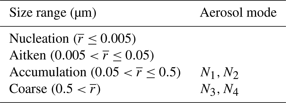
The modal structure of HAM-lite is flexible. The number, size, and composition of modes can be chosen according to the computational resources and research question. Table 1 shows a possible configuration with four hydrophilic modes in the accumulation and coarse range. We acknowledge that the one-moment scheme HAM-lite has limitations in comparison to the two-moment scheme HAM. Since it carries no information about the aerosol size, there is no explicit representation of nucleation, growth, and aging. And there is no ability to adjust the aerosol size in response to activation and wet deposition (Stier et al., 2005; Siebesma et al., 2020).

2.2 Atmospheric processes

The prognostic tracers that represent aerosols are transported through the atmosphere and influenced by various processes such as convection or precipitation. Figure 1 shows the prognostic variables and their spatial discretization in the Earth system model ICON-MPIM. The prognostic variables are the virtual temperature θ_v, air density ρ_a, horizontal and vertical velocities v_n and w, and tracers q_i. The tracers represent mixing ratios of water species or aerosols with respect to air mass. Horizontally, the atmosphere is discretized with an icosahedral–triangular C grid. Vertically, the atmosphere is divided into levels based on terrain-following coordinates (Giorgetta et al., 2018; Hohenegger et al., 2023).

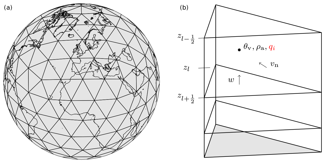
Figure 1 Spatial discretization and prognostic variables: icosahedral grid with equilateral triangles (a) and vertical column with full and half levels (b). Prognostic tracers that belong to the cloud or aerosol scheme are highlighted in red.

Small-scale processes within a grid cell need to be parameterized. These parameterized processes impose tendencies on the prognostic variables. There are three parameterization schemes: one for cloud microphysics, one for radiation, and one for turbulence, as shown in Fig. 2 adapted from Hohenegger et al. (2023). Cloud microphysics are parameterized with the one-moment scheme from Baldauf et al. (2011). The scheme computes specific masses of six water classes, i.e., water vapor, cloud water, cloud ice, rain, snow, and graupel. The cloud droplet number and ice particle number are not prognostic but prescribed or diagnosed. Radiation is parameterized with the radiative transfer scheme from Pincus et al. (2019). The scheme computes radiative properties and fluxes over 14 shortwave bands and 16 longwave bands. As shown in Fig. 2, it is called less frequently than the other schemes due to its computational complexity. Lastly, the turbulence is parameterized with the Smagorinsky scheme implemented by Dipankar et al. (2015). Surface fluxes are computed in coordination with the land scheme JSBACH from Reick et al. (2021).

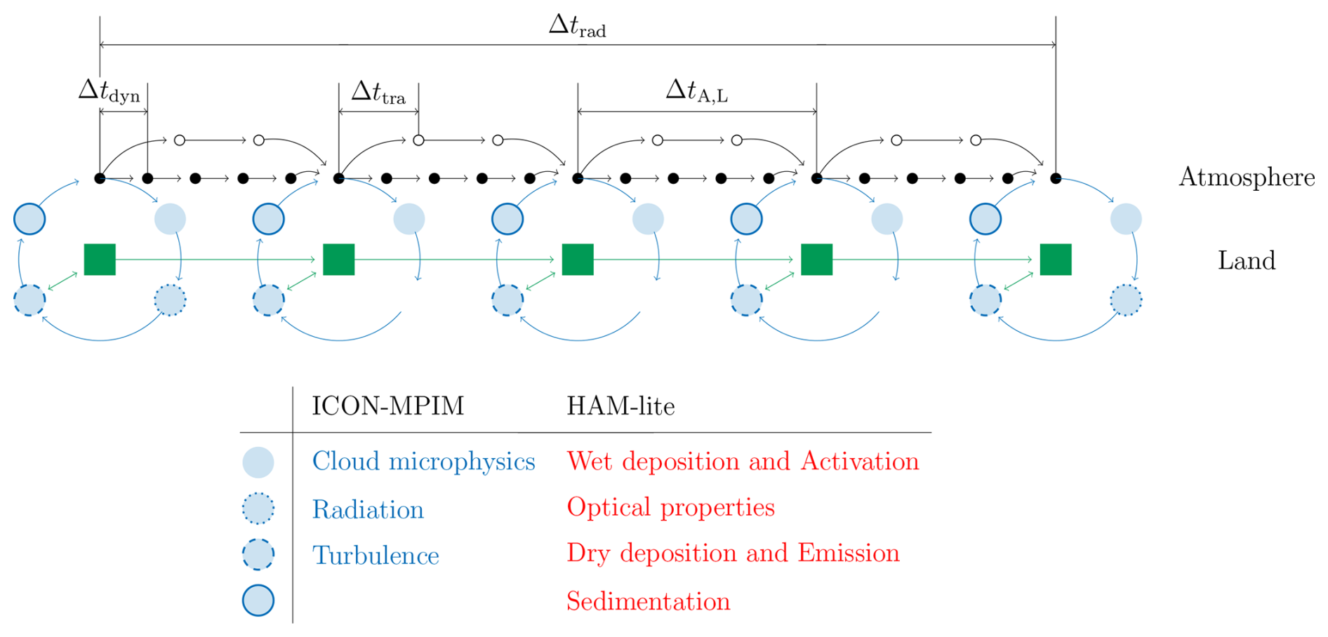
Figure 2 Time stepping (top) and parameterized processes (bottom): dynamical core and tracer transport (black), parameterized processes (blue), and land scheme (green). Processes of ICON-MPIM are highlighted in blue, and processes of HAM-lite are highlighted in red.

Partially resolved processes such as shallow convection or orographic drag are not parameterized. As outlined by Hohenegger et al. (2023), there are three main reasons for this choice. First, a lean code with few parameterization schemes can be ported more easily to new systems such as the new exascale cluster of the Forschungszentrum Jülich (2025). Second, parameterization schemes do not converge as the resolution is refined, which would be problematic for future simulations with ever increasing resolutions. Hohenegger et al. (2020) showed that some large-scale quantities such as net shortwave radiation start to converge at resolutions of about 5 km. Third, ICON-MPIM is intended for Earth system research and not operational weather forecasting. Simple physics make it easier to understand, for example, the impact of processes that remain partially resolved or parameterized at kilometer scales.

2.3 Aerosol processes

The aerosol module interacts with these processes, for example, when cloud droplets form on aerosol particles or surface winds drive dust emissions. Figure 2 shows how the parameterization schemes of ICON-MPIM and HAM-lite are coupled to each other (Salzmann et al., 2022). Wet deposition and activation are linked to the cloud microphysics scheme, radiative properties of aerosols are factored into the radiation scheme, and dry deposition and emission are linked to the turbulence scheme. Sedimentation is called separately at the end of the cycle. In the next sections, we introduce the different schemes of HAM-lite. The schemes impose either surface fluxes (m⁻² s⁻¹) or tendencies (kg⁻¹ s⁻¹) on the aerosol tracers, which represent aerosol number per air mass (kg⁻¹). In order to simplify the notation, the indices of full and half levels, i.e., z_l and $z_{l\pm \mathrm{1}/\mathrm{2}}$, are omitted.

2.3.1 Emission

Emissions are computed interactively or prescribed based on emission scenarios. Due to the absence of microphysical processes, emissions are directly added to modes without any intermediate steps. In reality, precursor gases such as sulfur dioxide form secondary aerosols by nucleation (Siebesma et al., 2020). Sea salt emissions are imposed as surface fluxes and computed based on a scheme of Gong (2003), taking into account the surface wind speed and sea surface temperature. Dust emissions are also imposed as surface fluxes and computed based on a scheme of Tegen et al. (2002), taking into account the surface wind speed and various surface properties provided by the land scheme. The emissions of sulfate, organic carbon, and black carbon are imposed as surface fluxes or tendencies and taken from the AeroCom-II ACCMIP database (Heil et al., 2022). It provides monthly averages of emissions from anthropogenic sources and biomass burning (Salzmann et al., 2022). The emissions are grouped into emission sectors such as forest fires or energy production. The emission sectors are attributed to different aerosol modes. The mass fluxes from the emission sectors are converted into number fluxes based on the radius of average mass of the mode, i.e.,

$$\begin{array}{}\text{(5)}& F_{\mathrm{em},j,k,s}={\displaystyle \frac{\mathrm{3}}{\mathrm{4}\mathit{\pi }{\stackrel{\mathrm{‾}}{r}}_{\mathrm{m},j}^{\mathrm{3}}{\mathit{\rho }}_k}}{S}_{\mathrm{em},k,s},\end{array}$$

where $S_{\mathrm{em},k,s}$ is the mass flux of species k in sector s. Note that the mass fluxes from the dust and sea salt emission schemes are converted in the same manner. The number fluxes are then added together such that the total number flux reads

$$\begin{array}{}\text{(6)}& F_{\mathrm{em},j}=\sum _{k=\mathrm{1}}^K\sum _{s=\mathrm{1}}^S{F}_{\mathrm{em},j,k,s},\end{array}$$

where S is the number of sectors that belong to the mode. The composition of a mixed mode with prescribed emissions can be derived from its number fluxes. The volume fraction of species j in mode k reads

$$\begin{array}{}\text{(7)}& {\mathit{\alpha }}_{j,k}={\displaystyle \frac{{\sum }_{s=\mathrm{1}}^S{N}_{\mathrm{em},j,k,s}}{{\sum }_{k=\mathrm{1}}^K{\sum }_{s=\mathrm{1}}^S{N}_{\mathrm{em},j,k,s}}},\end{array}$$

where $N_{\mathrm{em},j,k,s}$ is the total number of particles emitted over the simulation period. Since the fluxes are prescribed, the volume fractions can be computed once at the initialization stage.

2.3.2 Sedimentation

The sedimentation tendency is computed on all levels throughout the column as

$$\begin{array}{}\text{(8)}& F_{\mathrm{se},j}=q_j{v}_{\mathrm{se},j}/\mathrm{\Delta }z,\end{array}$$

in which q_j is the number mixing ratio, v_se,j is the sedimentation velocity, and $\mathrm{\Delta }z=z_{l+\mathrm{1}}-z_l$ is the distance between two full levels. The sedimentation velocity is modeled based on Stokes theory (Seinfeld and Pandis, 2016), i.e.,

$$\begin{array}{}\text{(9)}& \begin{array}{rl}{v}_{\mathrm{se},j}& ={\displaystyle \frac{\mathrm{2}}{\mathrm{9}}}{\displaystyle \frac{g\left({\mathit{\rho }}_{\mathrm{w},j}-{\mathit{\rho }}_{\mathrm{a}}\right)r_{\mathrm{w},j}^{\mathrm{2}}}{{\mathit{\mu }}_{\mathrm{a}}}}\\ & \left(\exp \left(\mathrm{2}{\ln }^{\mathrm{2}}{\mathit{\sigma }}_j\right)+\mathrm{1.246}{\displaystyle \frac{{\mathit{\lambda }}_{\mathrm{a}}}{{\stackrel{\mathrm{‾}}{r}}_{\mathrm{w},j}}}\exp \left({\displaystyle \frac{{\ln }^{\mathrm{2}}{\mathit{\sigma }}_j}{\mathrm{2}}}\right)\right),\end{array}\end{array}$$

in which g is the gravitational acceleration and λ_a is the mean free path. The term on the second line accounts for non-continuum effects following Riemer (2002). To ensure numerical stability, the velocity is limited to $\mathrm{\Delta }z/\mathrm{\Delta }{t}_{\mathrm{A},\mathrm{L}}$. Note that sedimentation to the surface is handled by the dry deposition scheme introduced in the next section.

2.3.3 Dry deposition

The dry deposition flux to the surface is computed as

$$\begin{array}{}\text{(10)}& F_{\mathrm{dd},j}={\mathit{\rho }}_{\mathrm{a}}{q}_j{v}_{\mathrm{dd},j},\end{array}$$

in which v_dd,j is the dry deposition velocity. It is formulated based on the scheme of Pleim et al. (2022), i.e.,

$$\begin{array}{}\text{(11)}& v_{\mathrm{dd},j}={\displaystyle \frac{v_{\mathrm{se},j}}{\mathrm{1}-\exp \left(-v_{\mathrm{se},j}\left(R_{\mathrm{ar}}+R_{\mathrm{ls},j}\right)\right)}},\end{array}$$

in which R_ar is the aerodynamic resistance and R_sf,j is the laminar sublayer resistance. The aerodynamic resistance reads

$$\begin{array}{}\text{(12)}& R_{\mathrm{ar}}={\displaystyle \frac{\mathrm{1}}{c_{\mathit{\kappa }}{u}_{\ast }}}\left(\ln \left({\displaystyle \frac{z_{\mathrm{sf}}}{z_{\mathrm{0}}}}\right)-{\mathrm{\Psi }}_{\mathrm{H}}\right),\end{array}$$

in which the von Kármán constant c_κ, friction velocity u_∗, and similarity profile $\left(\ln \right(z_{\mathrm{sf}}/z_{\mathrm{0}})-{\mathrm{\Psi }}_{\mathrm{H}})$ are taken from the turbulence scheme of ICON-MPIM (Dipankar et al., 2015). The laminar sublayer resistance reads

$$\begin{array}{}\text{(13)}& R_{\mathrm{ls},j}={\displaystyle \frac{\mathrm{1}}{{\mathit{ϵ}}_{\mathrm{ls}}{u}_{\ast }\left(E_{\mathrm{bd},j}+E_{\mathrm{im},j}\right)}},\end{array}$$

in which the ϵ_ls is an empirical correction, and E_bd,j and E_im,j are collection efficiencies due to Brownian diffusion and impaction. The empirical correction is equal to 1 for non-vegetated surfaces and equal to the leaf area index for vegetated surfaces. The vegetation fraction and leaf area index are provided by the land scheme. The collection efficiencies depend on the Stokes and Schmidt numbers. The Schmidt number reads $\mathit{Sc}={\mathit{\nu }}_{\mathrm{a}}/D_j$, in which ν_a is the kinematic viscosity of air and

$$\begin{array}{}\text{(14)}& \begin{array}{rl}{D}_j& ={\displaystyle \frac{k_{\mathrm{B}}{T}_{\mathrm{a}}}{\mathrm{6}\mathit{\pi }{\mathit{\mu }}_{\mathrm{a}}{\stackrel{\mathrm{‾}}{r}}_{\mathrm{w},j}}}\\ & \left(\exp \left({\displaystyle \frac{{\ln }^{\mathrm{2}}{\mathit{\sigma }}_j}{\mathrm{2}}}\right)+\mathrm{1.246}{\displaystyle \frac{{\mathit{\lambda }}_{\mathrm{a}}}{{\stackrel{\mathrm{‾}}{r}}_{\mathrm{w},j}}}\exp \left(\mathrm{2}{\ln }^{\mathrm{2}}{\mathit{\sigma }}_j\right)\right)\end{array}\end{array}$$

is the diffusion coefficient. Like the sedimentation velocity, it is corrected for non-continuum effects following Riemer (2002). The Stokes number reads ${\mathit{St}}_j={\mathit{\rho }}_{\mathrm{a}}{v}_{\mathrm{se},j}{u}_{\ast }^{\mathrm{2}}/\left(g{\mathit{\mu }}_{\mathrm{a}}\right)$ for non-vegetated surfaces and ${\mathit{St}}_j=v_{\mathrm{se},j}{u}_{\ast }/\left(g{A}_{\mathrm{co}}\right)$ for vegetated surfaces, in which A_co is the characteristic size of collectors like leaves or needles. It is assumed to be 10 mm for macroscale collectors and 1 µm for microscale collectors. To ensure numerical stability, the dry deposition velocity is limited to $\mathrm{\Delta }{z}_{\mathrm{sf}}/\mathrm{\Delta }{t}_{\mathrm{A},\mathrm{L}}$, where Δz_sf is the thickness of the surface layer and Δt_A,L is the time step of the atmosphere and land as shown in Fig. 2. The dry deposition flux is subtracted from the emission flux such that a net surface flux is returned to the turbulence scheme as indicated in Fig. 2.

2.3.4 Wet deposition

The wet deposition tendency is computed for all cloudy levels throughout the column as

$$\begin{array}{}\text{(15)}& \begin{array}{rl}{F}_{\mathrm{wd},j}& =q_j{f}_{\mathrm{ac},j}\left(z_{\mathrm{cb}}\right){\displaystyle \frac{q_{\mathrm{ra}}+q_{\mathrm{gr}}+q_{\mathrm{sn}}}{q_{\mathrm{cw}}+q_{\mathrm{ci}}+q_{\mathrm{ra}}+q_{\mathrm{gr}}+q_{\mathrm{sn}}}}\\ & {\displaystyle \frac{p_{\mathrm{ra}}+p_{\mathrm{gr}}+p_{\mathrm{sn}}}{\int \left(q_{\mathrm{ra}}+q_{\mathrm{gr}}+q_{\mathrm{sn}}\right){\mathit{\rho }}_{\mathrm{a}}\mathrm{d}z}},\end{array}\end{array}$$

in which f_ac,j is the fraction of activation at cloud base z_cb; q_cw, q_ci, q_ra, q_gr, and q_sn are the mass mixing ratios of cloud water, cloud ice, rain, graupel, and snow; and p_ra, p_gr, and p_sn are the precipitation rates of rain, graupel, and snow. The first term is the number of aerosols activated at cloud base. The second term on the first line is the ratio of the precipitating water classes and condensed water classes. It incorporates the fraction of condensed water that forms precipitation. And the third term on the second line is the ratio of the total surface precipitation and column integral over the precipitating water classes. It incorporates the fraction of precipitation that reaches the surface. A grid cell is assumed to be cloudy if its cloud water and ice is larger than 10⁻⁶ kg kg⁻¹. Note that the same threshold is used in the cloud microphysics scheme itself (Baldauf et al., 2011).

2.3.5 Activation

The fraction of activation is calculated with a scheme of Abdul-Razzak and Ghan (2000) based on the updraft velocity, wet diameter, and various other quantities. The activated particles of the different modes are then added together to obtain the cloud droplet number concentration:

$$\begin{array}{}\text{(16)}& N_{\mathrm{cd}}=\sum _{j=\mathrm{1}}^J{\mathit{\rho }}_{\mathrm{a}}\left(z_{\mathrm{cb}}\right)q_j\left(z_{\mathrm{cb}}\right)f_{\mathrm{ac},j}\left(z_{\mathrm{cb}}\right).\end{array}$$

Due to the limited resolution of a few kilometers, convective updrafts are only partially resolved. To account for that, the minimum number concentration is set to 30 cm⁻³ similarly to Goto et al. (2020), who used a lower bound of 25 cm⁻³. An alternative would be to implement a scheme for the unresolved updrafts as outlined by Malavelle et al. (2014). Note that the number concentration is used to calculate the autoconversion rate in the cloud microphysics scheme and the cloud optics in the radiation scheme (Seifert and Beheng, 2006; Pincus et al., 2019).

2.3.6 Optical properties

The aerosol optical properties are calculated on all levels according to Mie theory (Stier et al., 2005, 2007). They are extracted from look-up tables based on the standard deviation σ_j, Mie size parameter $X_j=\mathrm{2}\mathit{\pi }{\stackrel{\mathrm{‾}}{r}}_{\mathrm{w},j}/\mathit{\lambda }$, and refractive index ${\mathit{n}}_j=n_{\mathrm{real},j}+\mathrm{i}{n}_{\mathrm{imag},j}$. Similar to the other particle properties, the real and imaginary parts of the refractive index are computed as volume-weighted averages over the individual species including water such that

$$\begin{array}{}\text{(17)}& n_{\mathrm{real},j}={\displaystyle \frac{{\sum }_{k=\mathrm{1}}^K{V}_{j,k}{n}_{\mathrm{real},k}+V_{j,\mathrm{wa}}{n}_{\mathrm{real},\mathrm{wa}}}{{\sum }_{k=\mathrm{1}}^K{V}_{j,k}+V_{j,\mathrm{wa}}}}\end{array}$$

and

$$\begin{array}{}\text{(18)}& n_{\mathrm{imag},j}={\displaystyle \frac{{\sum }_{k=\mathrm{1}}^K{V}_{j,k}{n}_{\mathrm{imag},k}+V_{j,\mathrm{wa}}{n}_{\mathrm{imag},\mathrm{wa}}}{{\sum }_{k=\mathrm{1}}^K{V}_{j,k}+V_{\mathrm{wa},j}}}.\end{array}$$

The extinction coefficient C_ext,j, single-scattering albedo C_ssa,j, and asymmetry factor C_asy,j of the different modes are then combined to get bulk optical properties, i.e.,

$$\begin{array}{}\text{(19)}& {\displaystyle }{C}_{\mathrm{ext}}=\sum _{j=\mathrm{1}}^J{N}_j{C}_{\mathrm{ext},j},\text{(20)}& {\displaystyle }{C}_{\mathrm{ssa}}={\displaystyle \frac{{\sum }_{j=\mathrm{1}}^J{N}_j{C}_{\mathrm{ext},j}{C}_{\mathrm{ssa},j}}{C_{\mathrm{ext}}}},\end{array}$$

and

$$\begin{array}{}\text{(21)}& C_{\mathrm{asy}}={\displaystyle \frac{{\sum }_{j=\mathrm{1}}^J{N}_j{C}_{\mathrm{ext},j}{C}_{\mathrm{ssa},j}{C}_{\mathrm{asy},j}}{C_{\mathrm{ext}}{C}_{\mathrm{ssa}}}},\end{array}$$

in which N_j=ρ_aq_jΔz is the aerosol number in layer Δz. Note that the extinction coefficient is computed on longwave and shortwave bands, whereas the single-scattering albedo and asymmetry factor are computed only on shortwave bands (Bohren and Huffman, 1998; Siebesma et al., 2020).

3 Simulation setup

We performed a global simulation with ICON-MPIM together with HAM-lite at a resolution of 5 km over a period of 1 year. The simulation was configured as the cycle 3 simulation of nextGEMS (Koldunov et al., 2023). The sea surface temperature and sea ice were prescribed instead of simulating an interactive ocean, and the inhomogeneity factor for liquid clouds was adjusted to tune the radiation balance at the top of the atmosphere. The aerosols of HAM-lite were represented by four modes composed of dust, sea salt, organic carbon, black carbon, and sulfate.

Table 2 Aerosol composition and properties. Volume fractions (α_k) were derived from AeroCom-II ACCMIP (Heil et al., 2022). Dry radii ($\stackrel{\mathrm{‾}}{r}$) were adapted from MACv2 (Kinne, 2019). Densities (ρ) and hygroscopicities (κ) of species were taken from ECHAM6.3-HAM2.3 (Tegen et al., 2019) and GISS-E2.1-MATRIX (Fanourgakis et al., 2019). Standard deviations (σ) of modes were also taken from ECHAM6.3-HAM2.3, i.e., 2.00 for the dust and sea salt modes and 1.59 for the carbonaceous and sulfuric modes.

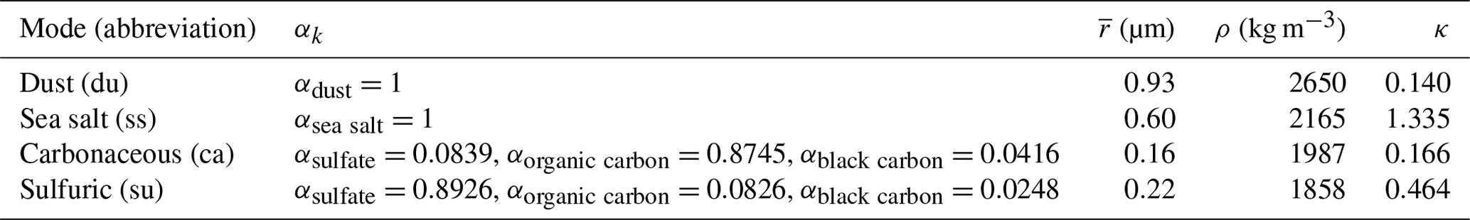
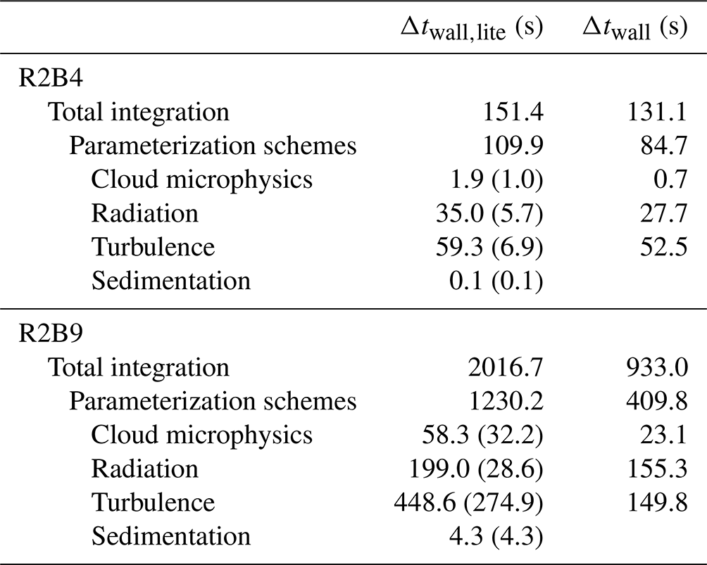
Table 3 Wall-clock times of 1 d with HAM-lite (Δt_wall,lite) and without HAM-lite (Δt_wall) at two different resolutions (R2B4 and R2B9). Due to fluctuations, the wall-clock times were averaged over three independent simulations. Input/output operations are not included. HAM-lite operations are given in brackets.

3.1 Model configuration

Horizontally, the atmosphere and land are discretized with the R2B9 grid, which corresponds to a grid spacing of about 5 km. Vertically, the atmosphere is divided into 90 levels with a thickness of 25–400 m, and the land is divided into five levels with a thickness of 0.065–5700 m. The time step of the atmosphere and land is $\mathrm{\Delta }{t}_{\mathrm{A},\mathrm{L}}=\mathrm{40}$ s and the time step of the radiation is Δt_rad=12 min. The initial conditions of the atmosphere and land were derived from the ERA5 reanalysis of the European Centre for Medium-Range Weather Forecasts (Hersbach et al., 2020). The boundary conditions for the ocean surface were taken from the AMIP II database (Taylor et al., 2000). The inhomogeneity factor for liquid clouds was increased from 0.4 to 0.8 in order to match the radiation balance at the top of the atmosphere with observations (Mauritsen et al., 2022). The simulation started on 20 January 2020 at 00:00 UTC and ran until 1 February 2021.

The aerosols are represented with four modes as summarized in Table 2. There are two pure modes, one of dust and one of sea salt, and two internally mixed modes, both of organic carbon, black carbon, and sulfate. The first mixed mode is dominated by carbon. It includes aerosols from forest fires, grass fires, agricultural waste burning, and biogenic emissions. The second mixed mode is dominated by sulfur. It includes aerosols from aviation, energy production and distribution, industry, maritime transport, land transport, waste treatment and disposal, residential and commercial combustion, and volcanoes. The emissions of the two mixed modes were taken from the AeroCom-II ACCMIP database following the RCP4.5 scenario (Heil et al., 2022). The biogenic emissions were taken from Guenther et al. (1995). As in HAM (Stier et al., 2005; Tegen et al., 2019), we assume that 15 % of biogenic monoterpene emissions form secondary organic aerosol (SOA) directly at the surface. We acknowledge that, in reality, SOA also forms above the surface. The densities and hygroscopicities of the species were taken from ECHAM6.3-HAM2.3 (Tegen et al., 2019) and GISS-E2.1-MATRIX (Fanourgakis et al., 2019). The dry radii of the modes were initially taken from the MACv2 aerosol climatology of Kinne (2019) and then adjusted to roughly match the aerosol lifetimes reported in Gliß et al. (2021). While the dry radii of the dust and sea salt modes were adjusted only marginally, the dry radii of the two carbonaceous and sulfuric modes were increased significantly since their initial lifetimes were too long. The simulation started from a clean atmosphere without aerosols.

3.2 Computational procedure

The simulation was performed and analyzed on the Levante cluster of the Deutsches Klimarechenzentrum GmbH (2024). The computational throughput was about 40 simulated days per day of wall-clock time on 400 compute nodes, each with 128 cores and 256 gigabytes of memory. A significant amount of the simulation time was related to input/output operations. One variable at one level and one time step requires about 0.08 gigabytes of disk space. In summary, we stored about 250 terabytes including some fields in three dimensions or at high frequency to track and analyze various processes.

To assess the computational costs related to HAM-lite, we performed test runs with and without interactive aerosols at two different resolutions, i.e., the coarse R2B4 grid on two nodes and the fine R2B9 grid on 400 nodes. Table 3 summarizes the wall-clock times of 1 simulated day without aerosols and with aerosols. It shows the total integration time but also a breakdown into parameterization schemes introduced in Sect. 2.2 and 2.3. Input/output operations such as reading of boundary conditions are not included. The simulation with aerosols was about 1.2 times slower on the R2B4 grid and about 2.2 times slower on the R2B9 grid. The operations of HAM-lite took a relatively small amount of time. The majority of the additional time was related to operations outside of HAM-lite such as tracer transport. There are 10 atmospheric tracers without aerosols compared to 14 atmospheric tracers with aerosols. And in contrast to the tracers of the cloud microphysics, the tracers of the aerosols are computed on all levels throughout the atmospheric column.

4 Results and discussion

Here, we present an initial analysis of the simulation outlined in Sect. 3. In the first part, we analyze the global aerosol cycle including burdens, lifetimes, fluxes, and optical depths. In the second part, we provide insights into regional processes such as the emission of dust aerosols by cold pool outflows in the Sahara or the interaction of sea salt aerosols and shallow convective storms around the doldrums.

Table 4 Global mean aerosol burdens and fluxes of ICON-HAM-lite averaged over February 2020 to January 2021 and of ECHAM6.3–HAM2.3 (CLIM simulation) averaged over the years 2003 to 2012 (Tegen et al., 2019).

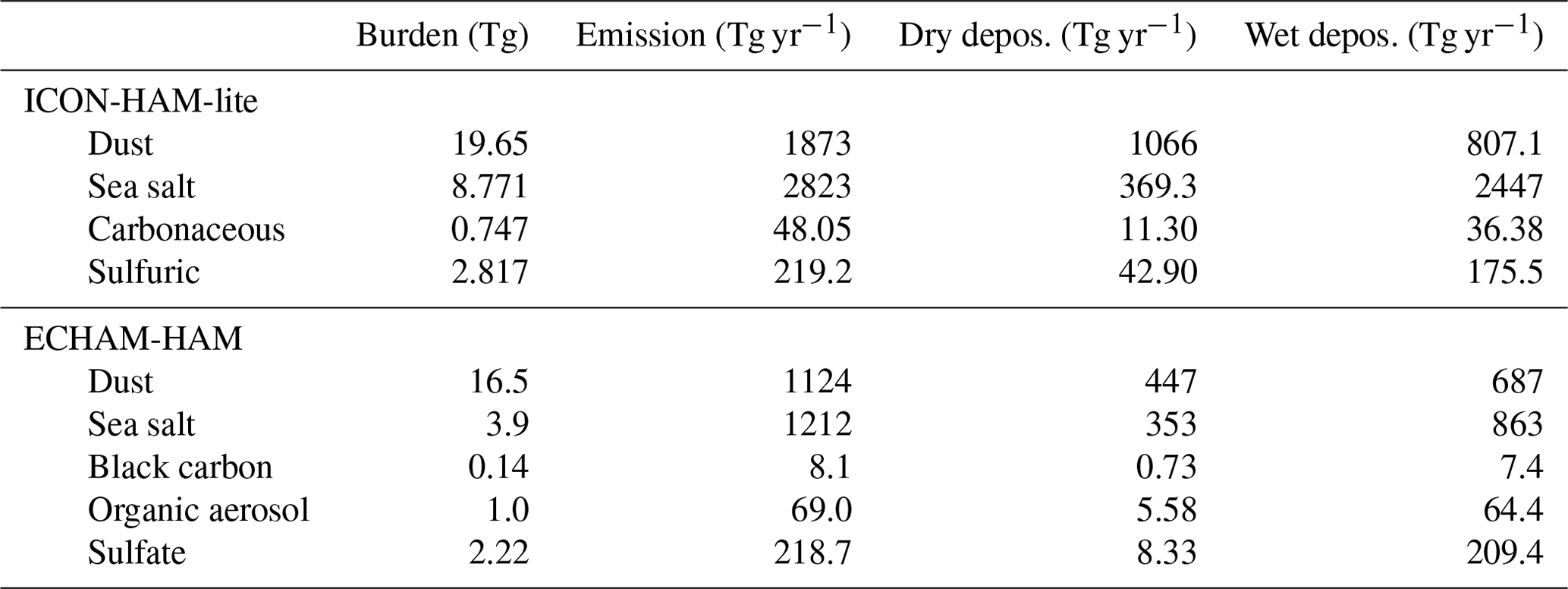
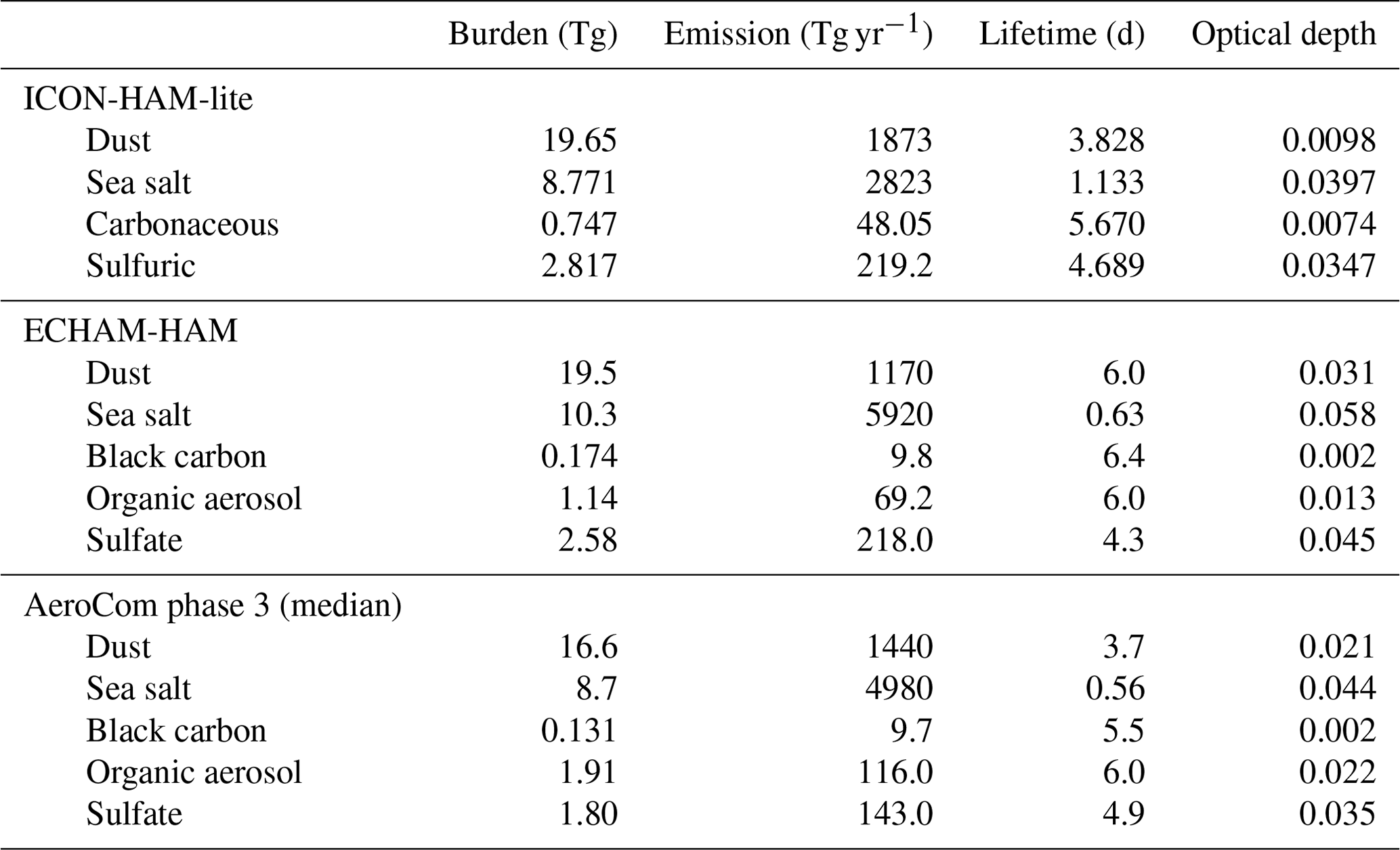
Table 5 Global mean aerosol burdens, emissions, lifetimes, and optical depths at 550 nm of ICON-HAM-lite averaged over February 2020 to January 2021 and of ECHAM6.3–HAM2.3 and AeroCom phase 3 averaged over the year 2010 (Gliß et al., 2021).

4.1 Global cycle

To start with, we evaluate the global cycle of aerosols averaged over 1 year from February 2020 to January 2021. Due to the large computational costs, we discard only the first 12 d from 20 January to 1 February 2020 as spin-up time. Table 4 shows the aerosol burdens and fluxes of our simulation and of the CLIM simulation with ECHAM6.3-HAM2.3 averaged over the years 2003 to 2012 (Tegen et al., 2019). Table 5 shows the aerosol burdens, emissions, lifetimes, and optical depths at 550 nm of our simulation and of the AeroCom phase 3 model intercomparison, including ECHAM6.3-HAM2.3, averaged over the year 2010 (Gliß et al., 2021). ECHAM6.3-HAM2.3 used different sea salt emission schemes in the two studies, leading to differences in the sea salt emissions and burdens. The values of AeroCom, comparing more than 10 models, are subject to large uncertainties. For example, the standard deviations of the lifetimes range between 29 % for organic aerosol and 91 % for sea salt. Note that our lifetimes were estimated by dividing burdens with emission fluxes (Seinfeld and Pandis, 2016) and that our lifetimes are sensitive to the prescribed aerosol sizes listed in Table 2. In general, the size and lifetime of an aerosol are inversely related; i.e., a larger aerosol is activated and deposited more quickly than a smaller aerosol. Despite the simplicity of our model, our values are comparable to those of ECHAM6.3-HAM2.3 and AeroCom. The largest differences are observed for carbonaceous aerosols, which is caused by biomass burning emissions that are too low (Tegen et al., 2019; Salzmann et al., 2022). In future simulations, we plan to use wildfire emissions from the GFAS database (Kaiser et al., 2012) and anthropogenic emissions from the CEDS database (Hoesly et al., 2018; Feng et al., 2020), which are based on more recent observations and provided at higher resolutions than the AeroCom-II ACCMIP database (Heil et al., 2022).

To examine the distribution across the globe, Fig. 3 shows global maps of aerosol burdens averaged over 1 year. As expected, the column burden of dust is large over the deserts in North Africa, the Middle East, and East Asia. The column burden of sea salt is governed by the interplay of storm tracks and rain bands over the ocean. Sea salt aerosols are quickly washed out by marine clouds, and consequently their lifetime is about 1 d as shown in Table 5. The column burdens of the two mixed modes are governed by the emission scenario. Carbonaceous aerosols are concentrated over biomass burning regions, primarily in central Africa and East Asia, whereas sulfuric aerosols are concentrated over industrial regions, for example in China and India. To better understand emission and deposition, Fig. 4 shows global maps of the dust burden and fluxes. Dust aerosols are emitted by winds over the Sahara and Gobi desert. A large fraction of dust is deposited close to its source due its large radius and density given in Table 2. A smaller fraction is transported over longer distances, for example from the Sahara over the Atlantic and towards the Amazon.

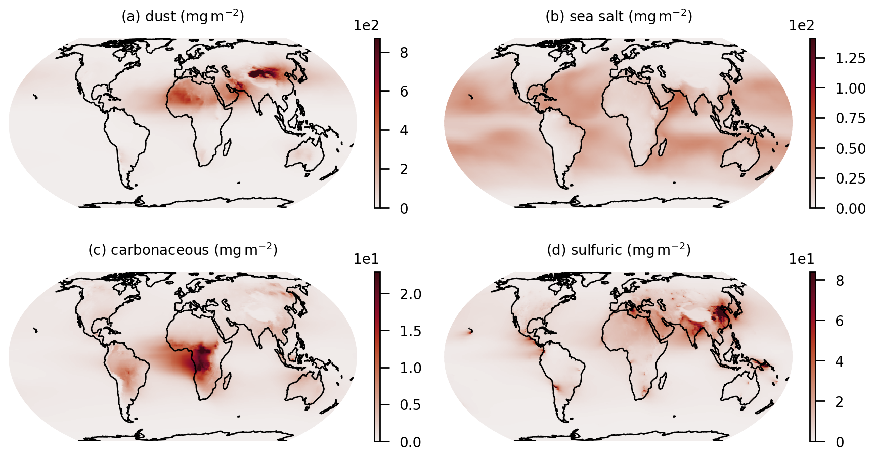
Figure 3 Column burdens of aerosols averaged over February 2020 to January 2021: dust (a), sea salt (b), carbonaceous aerosol (c), and sulfuric aerosol (d).

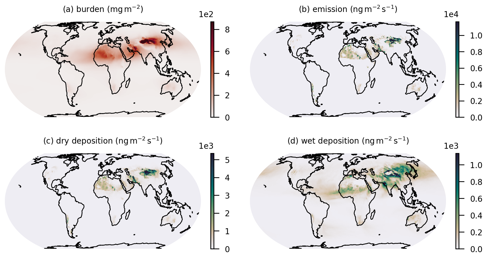
Figure 4 Column burden and fluxes of dust averaged over February 2020 to January 2021: burden (a), emission (b), dry deposition (c), and wet deposition (d).

To examine the distribution throughout the column, Fig. 5 shows global mean vertical profiles of aerosol mixing ratios averaged over 1 year. Dust aerosols are lifted up to about 6 km by convective storms, and some aerosols rise even further up to about 12 km. In contrast, sea salt aerosols are washed out by low marine clouds, and only few aerosols rise above 2 km. The profile of carbonaceous aerosols shows a local peak at about 14 km, whereas the profile of sulfuric aerosols decreases monotonically with the altitude. Carbonaceous aerosols have a smaller dry radius and hygroscopicity than sulfuric aerosols as summarized in Table 2. And consequently, carbonaceous aerosols are activated and deposited less effectively. Note that the vertical distribution of aerosols is weakly constrained by observations and highly variable among AeroCom models (Kipling et al., 2016; Koffi et al., 2016). Besides convective transport, microphysical and chemical processes such as condensation or coagulation play an important role (Watson-Parris et al., 2019).

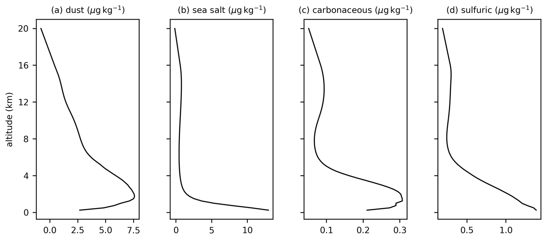
Figure 5 Global mean mass mixing ratios of aerosols averaged over February 2020 to January 2021: dust (a), sea salt (b), carbonaceous aerosol (c), and sulfuric aerosol (d).

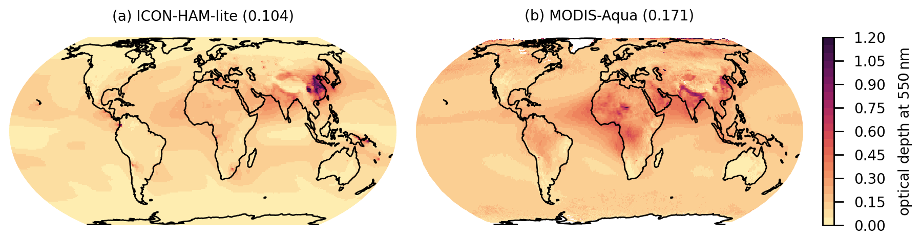
Figure 6 Aerosol optical depth at 550 nm of ICON-HAM-lite averaged over February 2020 to January 2021 (a) and of MODIS Aqua, i.e., the combined Dark Target and Deep Blue product (Platnick et al., 2015), averaged over 2018 to 2022 (b). The spatial average over 60° S to 60° N is given in brackets.

Finally, we evaluate the aerosol optical depth at 550 nm. Figure 6 shows the optical depth of our simulation and the MODIS Aqua satellite, i.e., the combined Dark Target and Deep Blue product (Platnick et al., 2015). The optical depth of our simulation was averaged over 1 year, whereas the optical depth of MODIS Aqua was averaged over 5 years from 2018 to 2022. Note that observations from satellites are subject to some uncertainties as discussed by Vogel et al. (2022). On average, the optical depth of MODIS is larger than those of other satellites, especially over the ocean (Vogel et al., 2022, their Tables 2 and 3). Within 60° S to 60° N, the average optical depth of our simulation (0.104) is lower than that of MODIS Aqua (0.171). Table 5 reveals that this bias is mainly related to the optical depths of carbonaceous and dust aerosols. The optical depths of these two modes are also lower than those of the MACv2 aerosol climatology of Kinne (2019), which is commonly used in simulations with ICON-MPIM (Hohenegger et al., 2023). The predefined optical depths are 0.031 for dust, 0.028 for sea salt, 0.022 for organic aerosol, and 0.037 for sulfate (Kinne, 2019, their Table 1). There are several ways to address these biases. First, we plan to revise the biomass burning emissions. As already mentioned, previous studies showed that those emissions are too low compared to observations (Kaiser et al., 2012; Tegen et al., 2019; Salzmann et al., 2022). Second, we plan to fine-tune the aerosol properties listed in Table 2. As already mentioned, the aerosol sizes have large impacts on the lifetimes and optical depths. Third, we plan to include secondary aerosols from nucleation (Stier et al., 2005). In addition, one could revise the removal processes, for example the resistances in the dry deposition scheme or the activation fraction in the wet deposition scheme.

4.2 Regional insights

After the global overview, we provide insights into regional processes that are only resolved in kilometer-scale simulations. Figure 7 shows a scene of aerosols and clouds on 10 August 2020 at 00:00 UTC. It shows the horizontal distribution of aerosol burdens as well as the vertical distribution of aerosols and cloud water and ice along the prime meridian. In order to show all modes in one frame, the color maps have a variable transparency. The images capture various processes in a new level of detail. Dust aerosols are lifted above 400 hPa by convective storms over the Sahara. Sea salt aerosols are washed out by low marine clouds below 800 hPa. Carbonaceous aerosols are emitted by wildfires, predominantly in central Africa and South America, and transported over the ocean by trade winds. And sulfuric aerosols are emitted by anthropogenic and volcanic activity and lifted up to 200 hPa.

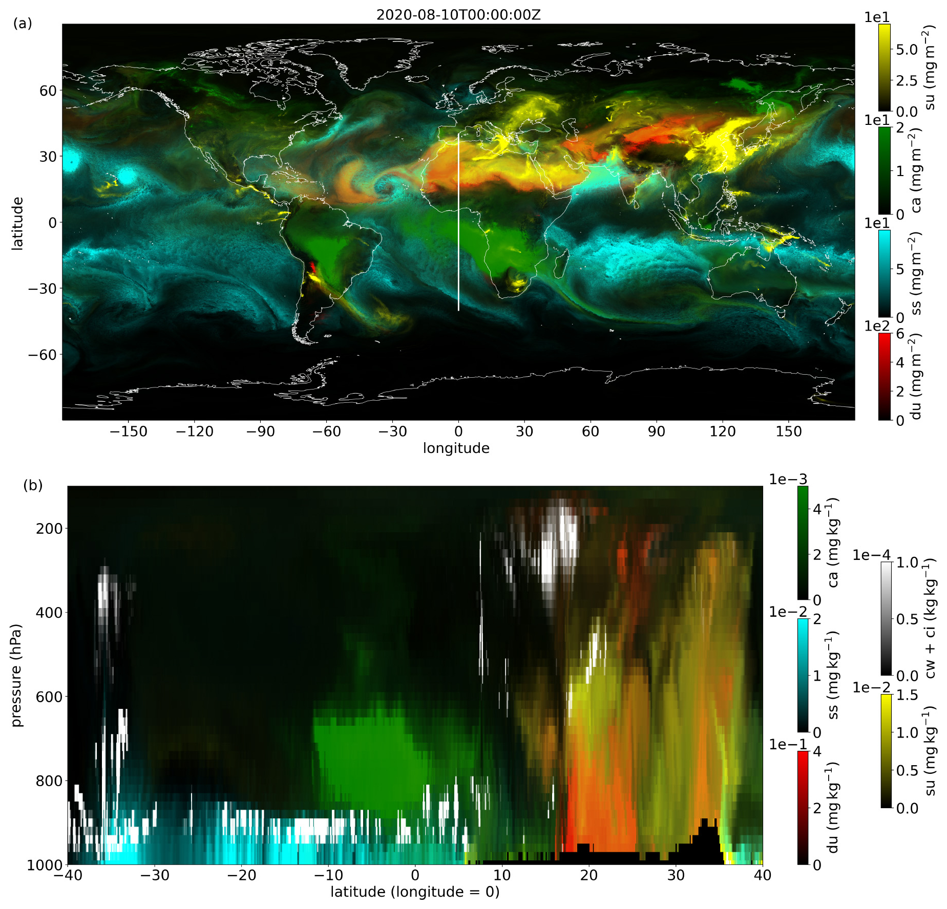
Figure 7 Scene of aerosols and clouds on 10 August 2020 at 00:00 UTC. Panel (a) shows column burdens of dust (du) in red, sea salt (ss) in blue, carbonaceous aerosol (ca) in green, and sulfuric aerosol (su) in yellow. Panel (b) shows the corresponding mass mixing ratios together with the mass mixing ratio of cloud water and ice (cw + ci) in white along the prime meridian indicated in (a). The color maps have a variable transparency which decreases from fully transparent at minima to fully opaque at maxima.

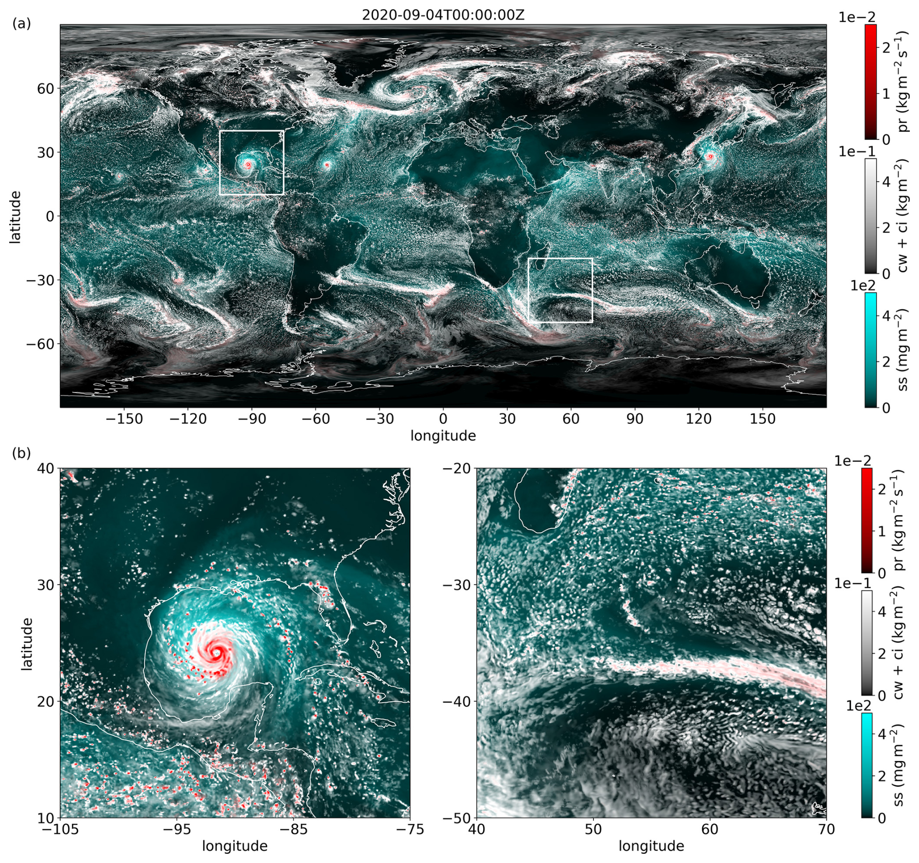
Figure 8 Scene of sea salt, cloud water and ice, and precipitation on 4 September 2020 at 00:00 UTC. Panel (a) shows the column burden of sea salt (ss) in blue, column burden of cloud water and ice (cw + ci) in white, and surface precipitation (pr) in red. Insets (b) show a tropical cyclone in the Gulf of Mexico and a weather front in the Indian Ocean. The color maps have a variable transparency which decreases from fully transparent at minima to fully opaque at maxima.

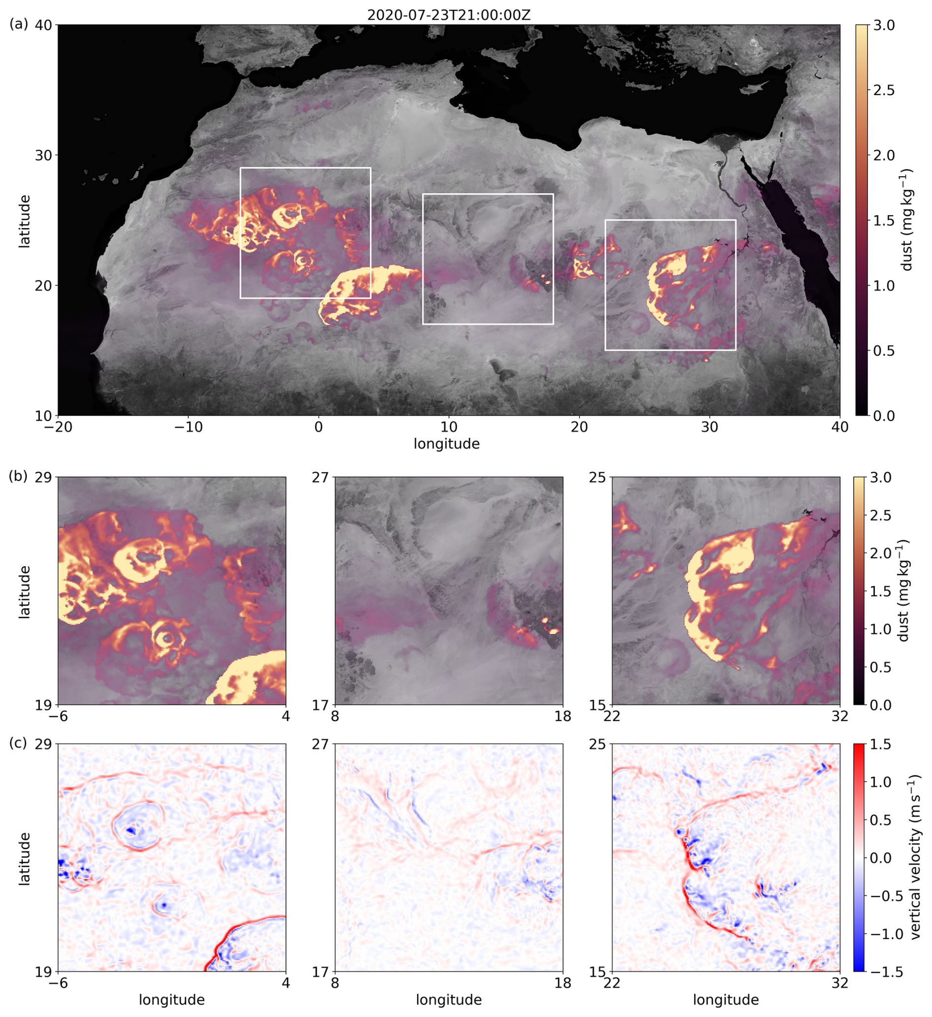
Figure 9 Scene of dust over the Sahara on 23 July 2020 at 21:00 UTC. Panel (a) and the insets in (b) show the mass mixing ratio of dust at the lowest model level above the surface. Insets in (c) show vertical velocity at 850 hPa. The color maps of (a) and the insets in (b) have a variable transparency which decreases from fully transparent at minima to fully opaque at maxima. The background is the Blue Marble composite of the NASA Earth Observatory (2024) converted to grayscale.

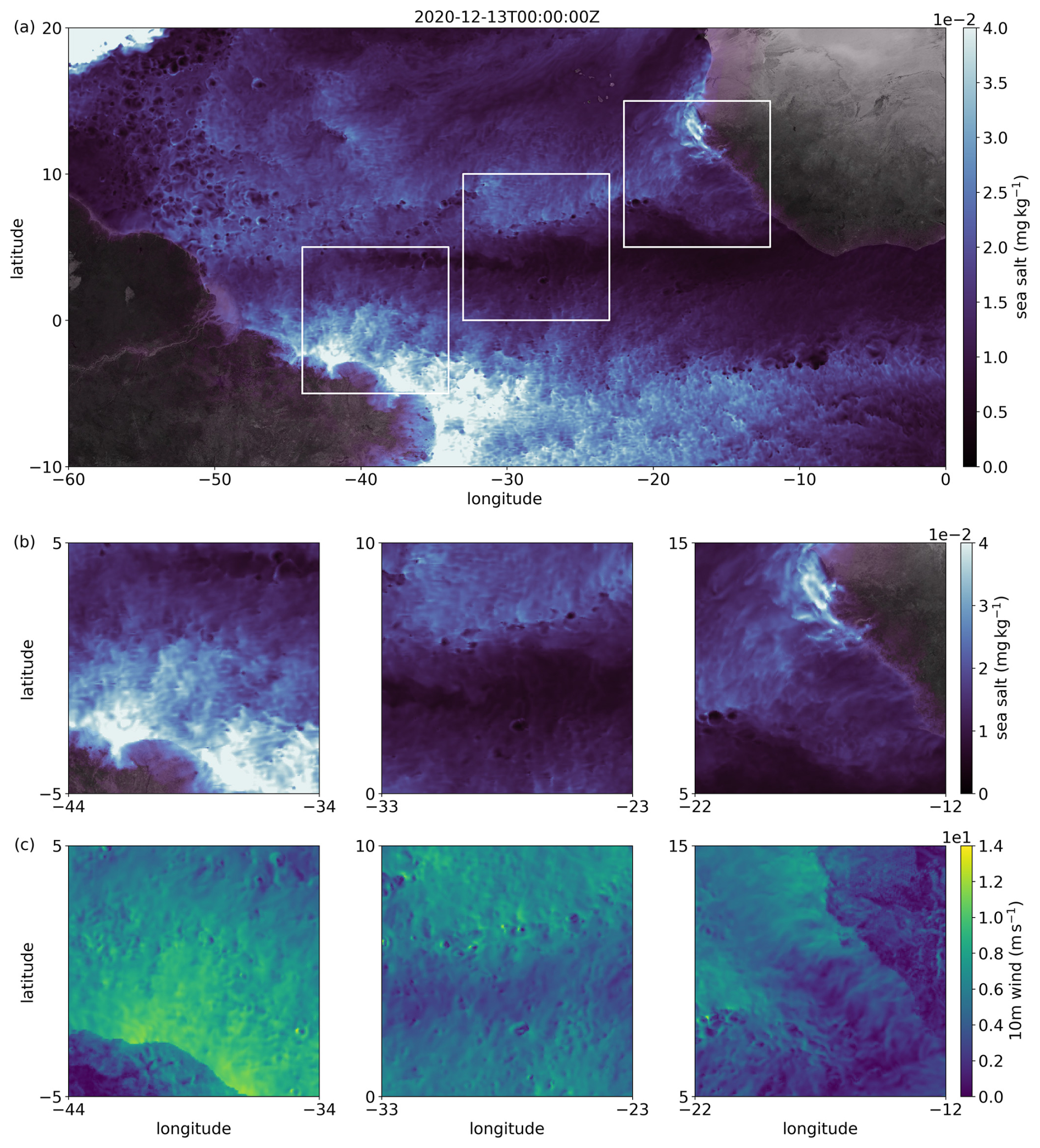
Figure 10 Scene of sea salt over the Atlantic on 13 December 2020 at 00:00 UTC. Panel (a) and the insets in (b) show the mass mixing ratio of sea salt at the lowest model level above the surface. Insets in (c) show wind speed at 10 m above the surface. The color maps of (a) and the insets in (b) have a variable transparency which decreases from fully transparent at minima to fully opaque at maxima. The background is the Blue Marble composite of the NASA Earth Observatory (2024) converted to grayscale.

To highlight the interaction of aerosols and clouds, Fig. 8 shows a scene of sea salt aerosols, cloud water and ice, and precipitation on 4 September 2020 at 00:00 UTC. It provides a global overview and highlights a tropical cyclone in the Atlantic and a weather front in the Indian Ocean. Like in Fig. 7, the color maps have a variable transparency. The global overview shows how sea salt aerosols are emitted by surface winds and deposited by rain bands. The distribution of sea salt aerosols is rather variable due to their short lifetimes of about 1 d. Low burdens can be seen, for example, in the Pacific or Southern Ocean, whereas high burdens can be seen in the Atlantic or Indian Ocean. The tropical cyclone is associated with large wind speeds, precipitation rates, and sea salt burdens. Previous studies have shown that aerosol–cloud interactions play an important role in cyclones, although these results were subject to model details such as the representation of cloud microphysics (Khain et al., 2016; Hoarau et al., 2018).

To highlight the interaction of convective storms and dust emissions, Fig. 9 shows a scene of dust aerosols over the Sahara on 23 July 2020 at 21:00 UTC. It shows the mass mixing ratios of dust at the lowest model level and the vertical velocities at 850 hPa. The vertical velocities highlight diverging cold pools that originate from convective downdrafts and mesoscale circulation that lifts air at the gust front. These cold pool outflows drive intense dust storms, also known as haboobs, that move towards the western coast. Haboobs generate a large fraction of the global dust burden and impact the global energy budget of Earth (Kok et al., 2023). Coarse-resolution models without resolved convection cannot capture mesoscale dynamics and the associated dust storms and need to compensate for that with the aid of tuning parameters (Marsham et al., 2011; Prein, 2023). This highlights the strong potential of kilometer-scale models to adequately represent small-scale processes that drive the global dust cycle (Heinold et al., 2013; Senior et al., 2021).

To highlight the interaction of surface winds and sea salt emissions, Fig. 10 shows a scene of sea salt aerosols over the Atlantic on 13 December 2020 at 00:00 UTC. It shows the mass mixing ratios of sea salt in the lowest model level and the wind speeds at 10 m above the surface. There are various small and large-scale features. The large area of high sea salt concentrations is related to persistent trade winds. The large band of low sea salt concentrations across the Atlantic reflects a large zone of calm winds, also known as doldrums. Despite its large extent, this zone is not captured accurately in coarse-resolution simulations. And lastly, the small circular features were caused by shallow convective storms or deep convective clusters associated with intense precipitation (Klocke et al., 2017).

5 Conclusion and outlook

We introduced a new one-moment aerosol module, HAM-lite, that is traceable to the two-moment module HAM (Stier et al., 2005; Salzmann et al., 2022). Aerosols are represented as an ensemble of lognormal modes with prescribed dry radius and standard deviation. The modal structure of HAM-lite is flexible. The size and composition of modes can be chosen according to the computational resources and research question. To test our module, we performed a year-long simulation with four idealized aerosol modes. There were two pure modes, one of dust and one of sea salt, and two internally mixed modes, both of organic carbon, black carbon, and sulfate. The atmosphere and land were resolved with a resolution of 5 km, and the sea surface temperature and sea ice were prescribed.

We presented an overview of the global aerosol cycle and provided insights into regional aerosol processes that are only resolved at kilometer scales. The global overview showed that the aerosol lifetimes are comparable to those reported in previous model intercomparisons (Textor et al., 2006; Gliß et al., 2021). The aerosol optical depth is, however, lower than expected, also in comparison with satellite observations (Vogel et al., 2022). To address this bias, we plan to update the biomass burning emissions and to revise the prescribed aerosol properties. The regional insights captured key aerosol processes at a new level of detail. Dust aerosols are lifted up by cold pool outflows in the Sahara and transported towards the Amazon. Sea salt aerosols are emitted by trade winds and washed out by low marine clouds. Carbonaceous aerosols are emitted from wildfires and transported over the ocean. Sulfuric aerosols are emitted from anthropogenic activities and transported across the Northern Hemisphere. These results demonstrate that kilometer-scale simulations with interactive aerosols are possible and that such simulations can provide new insights into the role of aerosols in the Earth system.

There are many plans and ideas for future research. We plan to evaluate the aerosol processes more in-depth, to update the emission database, to fine-tune parameters like aerosol size, and to add secondary aerosols from nucleation. In particular, we aim to improve the representation of the aerosol optical depth and absorption optical depth, which will be important for studies on aerosol forcing. On the model development side, we are cooperating with other groups to implement a new dust emission scheme from Klose et al. (2021), to include emissions of dimethyl sulfide (Fung et al., 2022), and to couple the aerosol module with the two-moment cloud microphysics scheme from Seifert and Beheng (2006), which would allow us to examine aerosol–cloud interactions in more detail. And on the scientific side, we plan to perform simulations with pre-industrial and present-day emission scenarios in order to estimate the effective radiative forcing (Forster et al., 2021), to analyze dust storms and deep convective clouds in a Lagrangian manner (Jones et al., 2024), and to compare our simulations with the incoming observations from the EarthCARE mission (Wehr et al., 2023).