GOSI9: UK Global Ocean and Sea Ice configurations

The UK Global Ocean and Sea Ice configuration version 9 (GOSI9) is a new traceable hierarchy of three model configurations at 1, $\mathrm{1}/\mathrm{4}$ and $\mathrm{1}/\mathrm{12}\mathit{°}$ based on version 4.0.4 of the NEMO code. GOSI9 has been developed as part of the UK's Joint Marine Modelling Programme (JMMP), a partnership between the Met Office, the National Oceanography Centre, the British Antarctic Survey, and the Centre for Polar Observation and Modelling. Following a seamless approach, it will be used for a variety of applications across a wide range of spatial and temporal resolutions: short-range coupled numerical weather prediction (NWP) forecasts, ocean forecasts, seasonal and decadal forecasts, and climate and Earth system modelling. The GOSI9 configurations are described in detail with a special focus on the updates since the previous version (GO6-GSI8). Results from 30-year ocean–ice integrations forced by CORE2 fluxes are presented for the three resolutions, and the impacts of the updates are assessed using the $\mathrm{1}/\mathrm{4}\mathit{°}$ integrations. The upgrade to NEMO 4.0.4 includes a new sea ice model SI³ (Sea Ice modelling Integrated Initiative) and faster integration achieved through the use of partially implicit schemes that allow a significant increase in the length of the time step. The quality of the simulations is generally improved compared to GO6-GSI8. The temperature and salinity drifts are largely reduced thanks to the upgrade to NEMO 4.0.4 and the adoption of fourth-order horizontal and vertical advections helping to reduce the numerical mixing. To improve the representation of the Southern Ocean, a scale-aware form of the Gent–McWilliams parameterization and the application of a partial-slip lateral boundary condition on momentum in the Southern Ocean have been added, resulting in a stronger and more realistic Antarctic Circumpolar Current (ACC) transport and a reduction in the temperature and salinity biases along the shelf of Antarctica. In the Arctic, the representation of sea ice is improved, leading to a reduction in surface temperature and salinity biases. In particular, the excessive and unrealistic Arctic summer sea ice melt in GO6-GSI8 is significantly improved in GOSI9 and can be attributed to the change in the sea ice model and to the higher albedos that increased sea ice thickness.

1 Introduction

The Joint Marine Modelling Programme (JMMP, 2024), founded in 2018, is a partnership between the Met Office and UK research centres: the National Oceanography Centre, the British Antarctic Survey, and the Centre for Polar Observation and Modelling. The JMMP's ambition is to provide national capability modelling infrastructure, configurations and model output to the UK community. Adopting the seamless forecasting approach (Brown et al., 2012), the JMMP global ocean and sea ice configurations are used for a variety of applications across a wide range of spatial and temporal resolutions: short-range coupled numerical weather prediction (NWP) forecasts, ocean forecasts, seasonal and decadal forecasts, and climate and Earth system modelling.

This paper describes the latest Global Ocean and Sea Ice configuration, GOSI9, based on the NEMO ocean modelling framework (Madec and NEMO system team, 2019). As for the previous global ocean configuration, GO6 (Storkey et al., 2018), GOSI9 is a traceable hierarchy of three resolutions: 1, $\mathrm{1}/\mathrm{4}$ and $\mathrm{1}/\mathrm{12}\mathit{°}$. Previously, new configurations of the Global Ocean (GO, Storkey et al., 2018; Megann et al., 2014) and Global Sea Ice (GSI, Ridley et al., 2018) were released separately, in part due to the dependence of the two models on different source codes. From NEMO version 4 (Madec and NEMO system team, 2019), the new native sea ice model SI³ (Sea Ice modelling Integrated Initiative) is available as part of the NEMO ocean modelling framework, and from this release onwards will be used for JMMP configurations. In the early stages of this development cycle, the configuration was referred to as GO8p[0-7], and some papers based on these pre-release versions may have used this naming convention. However, it was realized that the previous release of the sea ice component had already reached version 8, and a second release at version 8 could lead to confusion. To explicitly recognize the joint release of both ocean and sea ice components we have adopted a new nomenclature for joint releases, GOSI.

Development of new configurations is motivated primarily by the desire to improve the representation of the ocean and sea ice and secondarily to deliver better (more efficient) computational performance. The latter often comes from adopting newer code, whereas the former more frequently requires a combination of expert assessment to identify the cause of biases and to identify or write improved numerical schemes and an element of tuning or calibration to optimize the solution. Warm sea surface temperature (SST) biases in the Southern Ocean have been a long-standing issue in the Met Office coupled systems. In the Met Office GC3 coupled configuration (HadGEM3) based on the GO6+GSI8 ocean and sea ice components, the Southern Ocean SST bias was reduced compared with GC2 thanks to improved representation of clouds (Williams et al., 2018) and tuning of the isopycnal diffusion parameter (Storkey et al., 2018). However, a warm bias still remained (Roberts et al., 2019). Hewitt et al. (2016) and Roberts et al. (2019) looked at the representation of the Southern Ocean in the hierarchy of HadGEM3 coupled models. They highlight that the large biases in the Antarctic Circumpolar Current (ACC) transport reduced by 40 % compared to observations, especially in the $\mathrm{1}/\mathrm{4}\mathit{°}$ configuration, which has the lowest transport.

GOSI9 is required to deliver improved performance in both forced (ocean and sea ice only) and coupled configurations. It will form the ocean and sea ice component of the forthcoming GC5 version of the Met Office Hadley Centre coupled climate model (Xavier et al., 2023) and will be the physical basis of the next UKESM (Mulcahy et al., 2023). To mitigate the risk of having to introduce configuration changes late in the development cycle, a new approach was adopted: GOSI9 $\mathrm{1}/\mathrm{4}\mathit{°}$ was tested in a coupled configuration at an early stage during the development process. This revealed some key insights into potential mean state biases that we were then able to address during the cycle. We describe this process later, but the main focus of this paper is to present the results and testing of GOSI9 forced by atmospheric surface forcing. Evaluation of the final coupled configuration is presented in Xavier et al. (2023).

The paper is organized as follows. Section 2 provides a detailed description of the GOSI9 configurations and the developments introduced into the global ocean configurations since the previous release, GO6. Section 3 describes the model simulations presented in this study, including the forcing and initialization used. In Sect. 4 we present the results from the global evaluation for the three resolutions comparing GOSI9 and GO6, and the impact of individual changes are assessed using the $\mathrm{1}/\mathrm{4}\mathit{°}$ configuration. Section 5 provides a more detailed evaluation of three key regions of interest: the North Atlantic, the northwestern Pacific and the Southern Ocean.

2 Model description

GOSI9 is based on NEMO v4.0.4 (Madec and NEMO system team, 2019) and the SI³ sea ice component (Blockley et al., 2024) and is built on the traceable hierarchy of three model configurations at 1, $\mathrm{1}/\mathrm{4}$ and $\mathrm{1}/\mathrm{12}\mathit{°}$ horizontal resolution described in Storkey et al. (2018). For ease of reference, in this section we provide a complete description of GOSI9. Details of the configuration that remain common to GO6, namely the grids, bathymetries, free-surface solution and advection, and mixing and boundary conditions are described first. We then describe the developments that have been made since GO6. Together these define the GOSI9 configuration.

2.1 Model grids and bathymetries

The model grids and bathymetries are unchanged from GO6 (Storkey et al., 2018). For the three resolutions, the grids are based on the ORCA global grids available on the NEMO framework (Madec and NEMO system team, 2019). Therefore, eORCA1, eORCA025 and eORCA12 have a nominal 1, $\mathrm{1}/\mathrm{4}$ and $\mathrm{1}/\mathrm{12}\mathit{°}$ resolution at the Equator, respectively, and an isotropic Mercator grid (i.e. same zonal and meridional grid spacing). To avoid a singularity point in the ocean, in the Northern Hemisphere the grids are quasi-isotropic bipolar, with two north mesh poles being introduced on land in Siberia and Canada. To better represent the equatorial dynamics, from 20° N/S the eORCA1 model grid meridional resolution increases towards $\mathrm{1}/\mathrm{3}\mathit{°}$ at the Equator. In the Southern Hemisphere south of 67° S, the grid is extended to 85° S following the method described in Mathiot et al. (2017) to include ice shelf cavities.

The three models have the same vertical grid with 75 vertical levels. The level thickness is a double tanh function of depth increasing from 1 m thickness near the surface to 200 m at 6000 m depth. It provides a high resolution near the surface to resolve ocean responses to atmospheric forcing, including the diurnal cycle (Bernie et al., 2005) and a reasonable resolution at mid-depths for long-term climate responses. Stewart et al. (2017) show that 75 levels is the minimum number capable of resolving the second baroclinic mode and the surface layer. Partial step topography is used, making the depth of the bottom cell variable and adjustable to the real depth of the ocean (Adcroft et al., 1997; Barnier et al., 2006).

Different datasets were used to produce the model bathymetries for each resolution. In this regard, the hierarchy of resolutions is not fully traceable. For the 1° resolution model, eORCA1, the bathymetry is derived from ETOPO2 dataset (National Geophysical Data Center, 2006) with additional data from IBSCO (Arndt et al., 2013) on the Antarctic shelf. For the $\mathrm{1}/\mathrm{4}\mathit{°}$ resolution model, eORCA025, the bathymetry is derived from the ETOPO1 dataset (Amante and Eakins, 2009) with additional data from GEBCO (IOC et al., 2003) in coastal regions and from IBSCO (Arndt et al., 2013) on the Antarctic shelf. For the $\mathrm{1}/\mathrm{12}\mathit{°}$ resolution model, eORCA12, the bathymetry is derived from GEBCO_2014 (Weatherall et al., 2015). The bathymetry for eORCA025 had grid-scale smoothing applied. This was not done for the eORCA1 or eORCA12 bathymetries. A traceable set of bathymetries derived from a common source is planned for the next development cycle.

2.2 Free-surface solution and advection

As in GO6, in order to accurately represent the surface freshwater flux, the model uses a non-linear free surface allowing cell thicknesses throughout the water column to vary with time (z^* coordinate as in Adcroft and Campin, 2004). A change from GO6 (Storkey et al., 2018), in which a time-filtering solution was used with the fastest waves being filtered (Roullet and Madec, 2000), is that the equation of the surface pressure gradient is solved using the split-explicit free-surface formulation, also called the time-splitting formulation, following Shchepetkin and McWilliams (2005). The time-splitting solution allows for an explicit representation of the fastest external gravity waves.

For momentum advection, GOSI9 uses the vector-invariant form in which the horizontal advection is separated into rotational and irrotational terms. The vorticity term (including the Coriolis term) is calculated using the energy and enstrophy conserving scheme of Arakawa and Lamb (1981). In NEMO, different options of this scheme are available, differing in the way the topographic boundary condition is represented. We retain the option used in GO6, nn_een_e3f=0, which tends to reinforce the topostrophy of the flow (Madec and NEMO system team, 2019, Sect. 5.2.1). The irrotational part of the momentum advection is formulated according to Hollingsworth et al. (1983) in order to avoid near-grid-scale horizontal numerical instabilities (Ducousso et al., 2017). Advection of tracers is performed using the total variance diminishing (TVD) scheme of Zalesak (1979) with fourth-order advection in the horizontal and vertical directions. In GO6, the same scheme was used but with second-order advection in the horizontal and vertical directions.

2.3 Mixing and boundary conditions

Lateral diffusion of momentum is on geopotential surfaces and, as in GO6, uses a Laplacian viscosity in eORCA1 and a bi-Laplacian viscosity in eORCA025 and eORCA12. The coefficients are specified in Table 1. In the bi-Laplacian case, to prevent instabilities due to numerical diffusion, the viscosity coefficients reduce polewards with the cube of the grid length. For the eORCA1 model, the viscosity coefficients reduce linearly with the increased meridional grid spacing towards the Equator but are constant poleward of 20° N/S. This was an error in the input file that remains unchanged from GO6 and was identified too late in the development cycle to redress. Grid-space-dependent values have been tested and found to give small improvements in model fidelity. A modification to the input file similar to that applied by Hutchinson et al. (2023) will be necessary for applications in which the Antarctic ice shelf cavities are opened.

Table 1 Parameter changes between eORCA1, eORCA025 and eORCA12 configurations. The coefficient are calculated at the Equator. In the bi-Laplacian case (eORCA025 and eORCA12), the viscosity coefficients reduce polewards with the cube of the grid length. For the eORCA1 model, the viscosity coefficients reduce linearly with the increased meridional grid spacing towards the Equator but are constant poleward of 20° N/S (see Sect. 2.3). The coefficients are unchanged compared to GO6 (see Table 1 in Storkey et al., 2018).

Lateral diffusion of tracers is performed along isoneutral surfaces using Laplacian mixing with coefficients given in Table 1. A parameterization of adiabatic eddy mixing (Gent and Mcwilliams, 1990) with a spatially varying coefficient (Held and Larichev, 1996; Tréguier et al., 1997) is used in eORCA1. A weak grid-scale-aware Gent and Mcwilliams (1990) parameterization is now applied at the higher resolutions (see Sect. 2.5.6).

The mixing parameterizations are mainly unchanged compared to GO6. The vertical mixing of tracers and momentum is parameterized using a modified version of the Gaspar et al. (1990) turbulent kinetic energy (TKE) scheme (Madec and NEMO system team, 2019). To represent unresolved mixing due to internal wave breaking, a background vertical eddy diffusivity and a background viscosity are both applied. The background vertical eddy diffusivity has a value of $\mathrm{1.2}\times {\mathrm{10}}^{-\mathrm{5}}$ m² s⁻¹, which decreases linearly from ±15° latitude to a value of $\mathrm{1.2}\times {\mathrm{10}}^{-\mathrm{6}}$ m² s⁻¹ at ±5° latitude (Gregg et al., 2003). The background viscosity is applied globally with a constant value of $\mathrm{1.2}\times {\mathrm{10}}^{-\mathrm{4}}$ m² s⁻¹. Other unresolved processes are represented using parameterizations available in NEMO. Surface wave breaking mixing is parameterized following Craig and Banner (1994), increasing the mixing at the surface. Axell (2002) is used to represent the Langmuir cell mixing. An ad hoc parameterization is used to represent the mixing due to near-inertial wave breaking (Rodgers et al., 2014) with a length scale that can be varied geographically. Extensive work was carried to tune this length scale in GO6 (Storkey et al., 2018). Additional tuning was carried out during the development of GOSI9 in order to reduce biases in the coupled configuration (see Sect. 2.5.8).

To parameterize the convection, an increased vertical diffusivity of 10 m² s⁻¹ is applied where the water column becomes unstable. The double diffusive mixing is parameterized using Merryfield et al. (1999). A climatological geothermal heat flux (Stein and Stein, 1992) is added as a bottom boundary condition. A quadratic bottom friction is used globally with enhanced coefficient in the Indonesian Throughflow, Denmark Strait and Bab-el-Mandeb regions. Following Beckmann and Döscher (1997), an advective and diffusive bottom boundary layer scheme is used. The tidal mixing is parameterized following Simmons et al. (2004) with a special formulation for the Indonesian Throughflow as recommended by Koch-Larrouy et al. (2008).

2.4 Freshwater input from land

Freshwater flux from the river runoffs is applied to the ocean surface layer. The freshwater runoffs are considered fresh and as having the same temperature as the local SST. In order to avoid instabilities caused by shallow fresh layers, the vertical mixing is increased to $\mathrm{2}\times {\mathrm{10}}^{-\mathrm{3}}$ m² s⁻¹ in the top 10 m of the water column at runoff locations. Along Antarctica, to represent the ice sheet freshwater input, we apply a parameterization of ice shelf basal melting. Following Mathiot et al. (2017), climatological freshwater input is prescribed at the edge of the ice shelves through depth to mirror the effect of ice shelf basal melt on the circulation. Due to stability issues in GOSI9 we use iceberg melt climatology based on GO6 integrations instead of interactive icebergs (see Sect. 2.5.7).

2.5 Development and changes since GO6

2.5.1 Upgrade to NEMO 4.0.4

For GOSI9, the version of the NEMO code has been upgraded to NEMO 4.0.4 (compared to NEMO 3.6 for GO6). NEMO 4.0 was released in 2019 (Madec and NEMO system team, 2019). GOSI9 uses a split-explicit free surface proposed by Shchepetkin and McWilliams (2005). With the time-splitting solution, external gravity waves are explicitly represented. GO6 used the filtered free surface available at NEMO v3.6 (Roullet and Madec, 2000) in which the fastest waves are filtered. With the time-splitting solution the fast barotropic motions (such as tides) are also simulated with better accuracy. In NEMO4.0, the lateral-diffusion code has been rewritten with a different formulation including scale-aware setting of eddy viscosity and diffusivity.

The AeroBULK package (Brodeau et al., 2017) has been implemented in NEMO 4.0. With AeroBULK, four bulk formulations are available in NEMO. GOSI9 uses the NCAR formulation (formerly CORE) appropriate for forcing the model with the CORE2 dataset, the same formulation used in GO6, but AeroBULK provides some refinements with the computation of the air density and with the reduction in approximation in the estimation of surface-specific humidity of saturation by adding a dependence on the sea level pressure.

2.5.2 Sea ice model SI³

The sea ice component of GOSI9 is based upon NEMO's new native sea ice model, SI³ (Sea Ice modelling Integrated Initiative). SI³ is a dynamic–thermodynamic continuum sea ice model that includes an ice thickness distribution (ITD), conservation of horizontal momentum, an elastic–viscous–plastic (EVP) rheology and energy-conserving halo-thermodynamics (Vancoppenolle et al., 2023). SI³ has been available in the NEMO code since version 4.0, having been created by merging functionality from several different sea ice models used with NEMO (namely LIM, CICE and GELATO), building upon the LIM3 model of Rousset et al. (2015). SI³ is fully embedded within NEMO and is invoked from within NEMO's Surface Boundary Code (SBC) module.

Aside from the change in model, the physics of the sea ice component of GOSI9 are largely similar to those used in the previous GO6+GSI8 configuration (Ridley et al., 2018; Storkey et al., 2018) based upon CICE5. GOSI9 uses five thickness categories to model the sub-grid ITD, with an additional ice-free category for open water (Thorndike et al., 1975). Thermodynamic growth and melt of the sea ice is modelled using multi-layer thermodynamics, with four layers of ice and one of snow based upon Bitz and Lipscomb (1999). Sea ice dynamics are modelled using the elastic–viscous–plastic (EVP) rheology of Hunke and Dukowicz (2002). The biggest difference compared with GO6+GSI8 (Storkey et al., 2018) is the use of the broadband albedo scheme in SI3 instead of the dual-band scheme used in CICE. This has allowed us to tune the albedo independently of the coupled model, and we increased the values of the albedo relative to the SI3 defaults (ponded ice albedo is increased from 0.27 to 0.36, dry ice albedo is increased from 0.60 to 0.70 and dry snow albedo is increased from 0.85 to 0.87). The sea ice component of GOSI9 is run on the same model grid as the ocean and at every ocean time step. More details on the specifics of the sea ice configuration, along with details of how SI³ was adapted to work in the HadGEM3 coupled model, can be found in Blockley et al. (2024).

2.5.3 Equation of state TEOS-10

In GOSI9, the equation of state was upgraded to the Thermodynamic Equation Of Seawater 2010 (TEOS-10, Ioc et al., 2010) instead of the previous standard, the 1980 equation of state (EOS-80). An important change is the use of absolute salinity and conservative temperature instead of practical salinity and potential temperature for EOS-80. TEOS-10 provides a complete thermodynamically consistent representation of all thermodynamic properties of seawater and allows for a more accurate representation of the heat content.

However, the use of TEOS-10 has an impact for users. For the FOAM ocean forecasting system, the observations assimilated in the system are EOS-80 variables, meaning that the model TEOS-10 variables need to be converted to EOS-80 prior to being passed to the observation operator. There is no practical impact on coupling with atmosphere and sea ice, as the sea surface conservative (TEOS-10) temperature is converted to potential (EOS-80) temperature before coupling when using NEMO with TEOS-10 equation of state.

Note that for this paper the conservative temperature and absolute salinity fields from GOSI9 have been converted to potential temperature and practical salinity to facilitate the comparison with GO6. The temperature and salinity results presented throughout this paper are the EOS-80 variables (potential temperature and practical salinity).

2.5.4 Time step and performance

A benefit of upgrading to NEMO 4 has been the implementation of the adaptive-implicit vertical advection (Shchepetkin, 2015). As for most ocean models, the time step in NEMO needs to satisfy multiple criteria to maintain numerical stability. The vertical Courant–Friedrichs–Lewy (CFL) criterion is commonly the most limiting and imposes time and space discretization constraints. Treating the vertical advection implicitly can reduce these restrictions but causes large dispersive errors. With adaptive-implicit vertical advection, the implicit scheme is only used in targeted areas where potential breaches of vertical CFL conditions occur. It allows a much longer time step while retaining the accuracy of the explicit scheme.

Adaptive-implicit vertical advection has been introduced in the GOSI9 configurations in addition to an implicit sea ice drag (available from NEMO 4.0.4). These changes allow the use of a considerably longer time step (Table 2) without introducing any significant changes or biases in the ocean and sea ice (not shown). The performances from GO6 configurations, as described in Storkey et al. (2018), and from GOSI9 configurations, as described in this paper, are summarized in Table 2. All the integrations were performed on a Cray X40 supercomputer using Intel Broadwell processors. For the $\mathrm{1}/\mathrm{4}\mathit{°}$ model eORCA025, the time step has been increased by 33 % for the ocean-only configuration and by 50 % for the coupled GC5 configuration. For the $\mathrm{1}/\mathrm{12}\mathit{°}$ configuration eORCA12, the time step has been increased by 100 %, allowing for the production of 2 years of simulation per day on 6150 cores. For the 1° configuration eORCA1, the time step has been increased by 33 %. Note that for GO6, the “land suppression” option available in NEMO (Madec and NEMO system team, 2019) was only used for the $\mathrm{1}/\mathrm{12}\mathit{°}$ configuration, whereas it was used for the three resolutions in GOSI9. The land suppression option excludes much of the global land area from the calculations, allowing us to reduce the number of cores required. This explains the significant reduction in the number of cores used to perform the GOSI9 integrations for the 1° and $\mathrm{1}/\mathrm{4}\mathit{°}$ resolutions.

Table 2 Summary of GO6 and GOSI9 performances for the three studied resolutions. The integrations used are the reference simulations described in this paper and in Storkey et al. (2018). The integrations were performed on a Cray XC40 supercomputer using Intel Broadwell processors. The number of cores are for NEMO-SI3 only and does not include XIOS cores. Note that we were not able to perform an additional integration to test GO6 eORCA12 performance in parallel to GOSI9 eORCA12.

2.5.5 Numerical mixing

Numerical mixing, caused mainly by truncations in the tracer advection scheme, is a recognized problem in ocean models. In models such as NEMO that use quasi-Eulerian vertical coordinates, it arises from errors in vertical advection associated with internal waves and tides and also results from horizontal tracer advection in regions with a high cell Reynolds number where the mesoscale is not well resolved, which are particularly extensive on a $\mathrm{1}/\mathrm{4}\mathit{°}$ grid at mid and high latitudes. Megann (2018) estimated the numerical mixing in a $\mathrm{1}/\mathrm{4}\mathit{°}$ GO5.0 NEMO configuration by evaluating an effective diffusivity from the density transformation rate and demonstrated that the effective diffusivity was over 5 times as large as the explicit diffusivity calculated in the model mixing scheme. Megann and Storkey (2021) found that increasing the viscosity in a $\mathrm{1}/\mathrm{4}\mathit{°}$ GO6, either by using larger values for the fixed biharmonic viscosity parameter or by changing to the Smagorinsky viscosity formulation, led to a reduction of between 10 % and 20 % in the effective diffusivity over much of the ocean interior, along with comparable reductions in temperature and salinity biases. The sole disadvantage of increased viscosity is a reduction in stability: in GO6, tripling the fixed viscosity required the time step to be reduced by 50 % from the default of 1350 s, while GOSI9 requires a 50 % reduction in time step from the default of 1800 s if either the fixed viscosity is doubled or the Smagorinsky scheme is selected. This increase in running cost ruled out the use of viscosity as a tool to reduce numerical mixing in coupled applications of this ocean configuration. The z time-filtered arbitrary Lagrangian–Eulerian coordinate (Leclair and Madec, 2011) has been shown to significantly reduce numerical mixing from internal waves and tides (Megann et al., 2022; Megann, 2024) and may be considered for inclusion in future global Global Ocean and Sea Ice configurations, although this again requires a reduced time step at present for stability.

As an alternative approach to reducing the numerical mixing resulting from advection in poorly resolved mesoscale flows, the tracer advection in both horizontal and vertical directions was changed from second-order (the default in GO6) to fourth-order advection. This incurred no significant penalties in run time and did not require any reduction in time step.

2.5.6 Southern Ocean tuning

As highlighted in Sect. 1, the HadGEM3 coupled models with eddy-permitting ($\mathrm{1}/\mathrm{4}\mathit{°}$) or eddy-resolving ($\mathrm{1}/\mathrm{12}\mathit{°}$) ocean resolution have a history of large-scale biases in the Southern Ocean. The largest biases appear at eddy-permitting resolution, which shows weak ACC transports (Hewitt et al., 2016; Roberts et al., 2019) and overly active subpolar gyres in the Weddell and Ross seas and biases in the temperatures and salinities on the Antarctic shelves. Experiments in the coupled model showed that these biases are linked and that a package of changes aimed at damping the overactive gyres also had the effect of improving the ACC transport and the shelf temperature and salinity biases. The work in the coupled model is described in more detail in Storkey et al. (2024), while in this paper (Sect. 5.1) we show the impact in the forced GOSI9 configurations.

The so-called Southern Ocean package of changes to the eddying models consists of the introduction of a scale-aware form of the Gent–McWilliams parameterization and the application of a partial-slip lateral boundary condition on momentum in the Southern Ocean.

Hallberg (2013) discusses ocean models that resolve eddies in parts of the domain but not in others. This is the case for the $\mathrm{1}/\mathrm{4}$ and $\mathrm{1}/\mathrm{12}\mathit{°}$ models presented here, in which eddies are well resolved at low latitudes but not at high latitudes due to the decrease in the Rossby radius of deformation with latitude (see Hallberg, 2013, Fig. 1). At GOSI9 we try to account for the effect of the unresolved eddies at high latitudes by introducing the same space- and time-dependent version of the Gent–McWilliams scheme (Tréguier et al., 1997) as used in the low-resolution model but with a coefficient that is capped to be zero at low latitudes, ramping up to a low value of 75 m² s⁻¹ at high latitudes.

As with GO6, a free-slip lateral boundary condition on momentum is applied at all resolutions. To further damp the Southern Ocean gyres in the $\mathrm{1}/\mathrm{4}\mathit{°}$ and $\mathrm{1}/\mathrm{12}\mathit{°}$ configurations, we increase the topographic drag by introducing a partial-slip boundary condition (see Madec and NEMO system team, 2019, Sect. 7.1) south of 50° S.

2.5.7 Iceberg climatology

GO6 (Storkey et al., 2018) uses a Lagrangian iceberg model (Bigg et al., 1997; Martin and Adcroft, 2010). The same Lagrangian iceberg model was deployed in GOSI9, but interactive icebergs caused stability problems. An initial stability issue caused by excess melting was resolved by changing the melting temperature of the iceberg to the freezing point.

Stability was especially an issue with the coupled configuration, GC5, where excess precipitation over Antarctica is balanced through the iceberg calving to conserve fresh water. At times this resulted in double the number of icebergs compared to the forced GOSI9, and accumulation of icebergs along the Antarctic Peninsula caused regular crashes. Work was carried out to improve realism and stability: implementation of calving distribution along the ice shelf rather than on a single point and implementation of a speed limiter for icebergs to prevent icebergs from travelling more than half a grid cell into the processor halo region in one time step. These changes reduced the frequency of crashes but not to a satisfactory level. It is hoped that further development can be done to improve stability.

In the meantime, a freshwater iceberg climatology is used instead of the Lagrangian iceberg model. Tests were carried out using the Antarctic icebergs melt climatology from Merino et al. (2016). However, the Merino et al. (2016) climatology does not include melt contributions from the Northern Hemisphere. Therefore, we built a monthly freshwater iceberg climatology using the iceberg freshwater outputs from 30-year integrations of GO6 (Storkey et al., 2018), which are initialized from EN4 climatology and start from a state of rest with no icebergs. It takes around 4 years for the number of icebergs and the iceberg melt to stabilize, so the first 5 years of the simulations were discarded to create the climatology. A freshwater iceberg melt climatology was created for each resolution: 1, $\mathrm{1}/\mathrm{4}$ and $\mathrm{1}/\mathrm{12}\mathit{°}$ from the corresponding GO6 runs. The heat content of the meltwater into the ocean is calculated using the freezing point temperature and the latent heat of melting is extracted from the ocean.

Figure S1 in the Supplement shows the annual mean freshwater flux from icebergs calculated from GO6 integrations. The distribution of iceberg melt is similar between the different resolutions. As the distribution depends closely on the circulation, the distribution for the higher resolution configuration features more small-scale results, with iceberg melt occurring closer to the coast. The eORCA1 iceberg melt climatology differs from the higher resolution in the Weddell Sea, which could be a consequence of the difference in circulation in that region.

2.5.8 Coupled model GC5 tuning

During the early testing phase with the coupled model GC5, biases arose in the Indian Ocean, with SST that was too cold and subsurface temperatures that were too warm. To better understand and to try to reduce these biases, several sensitivity experiments were carried out, and these resulted in two key changes: an increase in the globally uniform value of the chlorophyll concentration and a reduction in the TKE mixing depth between 10 and 40° S. Increasing the chlorophyll concentration acts to reduce the depth of the penetrating solar radiation, warming the surface layer and cooling the subsurface. The chlorophyll concentration was increased from 0.05 mg m⁻³ at GO6 to 0.1 mg m⁻³, which better matches the observed climatological value in the tropics. As part of the GO6 development, extensive work was carried out to tune the near-surface mixing (Storkey et al., 2018). Tuning of the e-folding length scale nn_htau associated with the parameterization of near-inertial wave breaking resulted in the choice of a larger length scale in the Southern Ocean (Storkey et al., 2018, Fig. 2), where summertime climatological (de Boyer Montégut et al., 2004) mixed layers are on average deeper than in the northern latitudes. Revisiting this work, we found that reducing the mixing depth between 10 and 40° S improved the warm subsurface bias in the Indian Ocean. The changes were tested in the forced $\mathrm{1}/\mathrm{4}\mathit{°}$ GOSI9 configuration before being implemented as standard in the three GOSI9 configurations. In future configurations, we plan to use a seasonal climatology of the chlorophyll concentration that will better represent the large variations associated with spring blooms.

3 Integrations

For the experiments described in this paper, the model initial conditions for temperature and salinity are from monthly climatologies based on EN4 objective analysis (Good et al., 2013) for the years 1995–2014. For the 30-year integrations presented in Sect. 4, the sea ice is initialized with a restart produced after 1 year of integration. The 1-year integration is initialized with temperature and salinity from EN4 climatology, and the sea ice initial state is calculated by SI³ from the initial temperature and salinity. The model is spun up from a state of rest.

GOSI9 integrations are forced over the period 1976–2005 by the CORE2 surface dataset (Large and Yeager, 2009) using the NCAR bulk formulae (Large and Yeager, 2009). Relative wind stress between the wind and the ocean current is used. As temporal resolution of the CORE2 forcing is not sufficient to resolve the diurnal forcing (Bernie et al., 2007), an artificial diurnal cycle is imposed on the daily mean shortwave fluxes. A sea surface salinity (SSS) restoration towards monthly mean climatology is applied with a −33.333 $\mathrm{mm}{\mathrm{d}}^{-\mathrm{1}}{\mathrm{psu}}^{-\mathrm{1}}$ restoring coefficient. A monthly climatology is applied for the freshwater flux from river runoff (Bourdallé-Badie and Treguier, 2006), icebergs (see Sect. 2.5.7) and ice shelves (Rignot et al., 2013).

Sensitivity experiments with the $\mathrm{1}/\mathrm{4}\mathit{°}$ configuration have been carried out to test the impact of changes detailed in Sect. 2.5. The list of experiments is detailed in Table 3. For all experiments, initialization and forcing follow the protocol used for GOSI9 and described above. Results from these experiments are assessed in Sect. 4. Mixed-layer depth climatology from the de Boyer Montégut et al. (2004) dataset, sea surface temperature climatology from ESA Climate Change Initiative (CCI) (Merchant et al., 2014), temperature and salinity climatologies from EN4 objective analyses (Good et al., 2013) are used for comparison. EN4 temperature and salinity are averaged over the period 1995–2014, covering a period where data from Argo floats are available.

Storkey et al. (2018)Storkey et al. (2018)Storkey et al. (2018)

Table 3 A list of experiments with eORCA025 configuration. “SO pack.” represents the Southern Ocean package, including GM eddy parameterization and increased topographic drag (see Sect. 2.5.6). “Adv. order” represents the order of the advection used in the model. The same order is used for the vertical and the horizontal advection. “Chl. conc.” represents the chlorophyll concentration. For all integrations, a constant is used.

4 Model evaluation and comparison with GO6

In this section, the results from the three GOSI9 integrations are evaluated and compared against the GO6 integrations and observation-based products.

4.1 Global drift and budget analysis

The first metrics used to evaluate the model performance are the drifts in the globally integrated temperature and salinity from the initial conditions (Figs. 1 and 2). Starting from an observed climatological state, the model should ideally exhibit no strong trend over time. Figures 1 and 2 compare the drifts in GO6 (left) and GOSI9 (right) for 1° (a, b), $\mathrm{1}/\mathrm{4}\mathit{°}$ (c, d) and $\mathrm{1}/\mathrm{12}\mathit{°}$ (e, f).

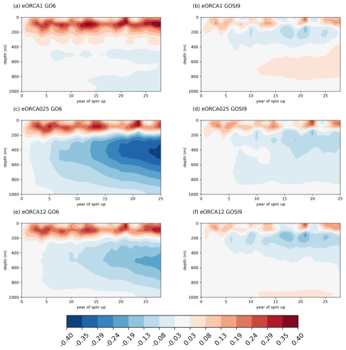
Figure 1 Global mean potential temperature drift from initial conditions (K) for GO6 (a, c, e) and GOSI9 (b, d, f).

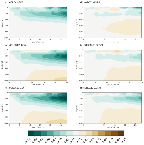
Figure 2 Global mean practical salinity drift from initial conditions for GO6 (a, c, e) and GOSI9 (b, d, f).

GOSI9 represents a substantial improvement in both temperature and salinity biases over the top 1000 m compared with GO6. The warm bias that was established quickly in the upper 300 m in GO6 is reduced to around one-third its size across the three resolutions, and the strong cooling that was manifest primarily in the $\mathrm{1}/\mathrm{4}\mathit{°}$ and $\mathrm{1}/\mathrm{12}\mathit{°}$ resolutions is far smaller. The improvements in the upper 300 m are largely attributable to the increase in chlorophyll concentration and the reduction in the mixing depth (see Sect. 2.5.8), while the reduction in the numerical mixing from using the fourth-order advection scheme and the upgrade to NEMO 4.0.4 are the leading contributors to the reduction in cooling below 300 m. Figure 3 shows an evolution of the globally integrated temperature drift from GO6 (a) through to GOSI9 (f) in the $\mathrm{1}/\mathrm{4}\mathit{°}$ configuration. Figure 3b–e show intermediate stages of the development process, enabling us to attribute relative contributions to the improvement of individual changes that have been made to the model configuration. The panels correspond to the list of experiments shown in Table 3.

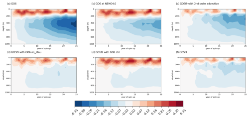
Figure 3 Global mean potential temperature drift from initial conditions (K) for the experiments with the $\mathrm{1}/\mathrm{4}\mathit{°}$ resolution model. (a) GO6. (b) GO6 4.0, which uses GO6 upgraded to NEMO 4.0.4; this configuration is the first experiment using the sea ice model SI³ and has large sea ice biases impacting the surface salinity. (c) GOSI9. (d) GOSI9 nn_etau, which uses GOSI9 with GO6 TKE mixing depth. (e) GOSI9 chl, which uses GOSI9 with GO6 chlorophyll concentration. (f) GOSI9 2nd order, which uses GOSI9 with second-order horizonal and vertical advection. The experiments are detailed in Table 3.

Similarly, the fresh bias that develops over the upper 500 m, centred around 200 m depth, is reduced by 50 % or more in GO6 (Fig. 2). This is mainly due to the upgrade to NEMO 4.0.4 (Fig. 4b) and the more accurate bulk formulae, which produce a salinification in the tropics. The other developments resulted in minimal impact on the globally integrated salinity trends (Fig. 4). While in GO6 the amplitude of the salinity and temperature drifts varies with the resolutions, all three GOSI9 models show consistent drift with little variation between resolutions.

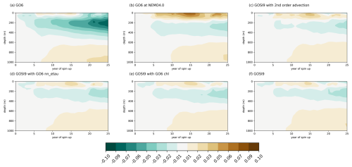
Figure 4 Global mean practical salinity drift from initial conditions (K) for the experiments with the $\mathrm{1}/\mathrm{4}\mathit{°}$ resolution model. (a) GO6. (b) GO6 4.0, which uses GO6 upgraded to NEMO 4.0.4; this configuration is the first experiment using the sea ice model SI³ and has large sea ice biases impacting the surface salinity. (c) GOSI9. (d) GOSI9 nn_etau, which uses GOSI9 with GO6 TKE mixing depth. (e) GOSI9 chl, which uses GOSI9 with GO6 chlorophyll concentration. (f) GOSI9 2nd order, which uses GOSI9 with second-order horizontal and vertical advection. The experiments are detailed in Table 3.

This assessment of model drift in globally integrated quantities is very positive, suggesting significant improvements over the previous generation of the models. However, we now need to assess whether these improvements arise from a reduction in biases or whether they are the product of large competing regional biases.

4.2 Large-scale biases

4.2.1 Zonal-mean biases

For the next assessment we compute zonal and time mean quantities of temperature and salinity using the period 1996–2005, the last decade of the forced simulations. Figure 5 shows anomalies of these metrics computed for the $\mathrm{1}/\mathrm{4}\mathit{°}$ configuration from both GO6 and GOSI9 from a reference 20-year climatology of EN4 v1.1 and anomalies between GOSI9 and GO6.

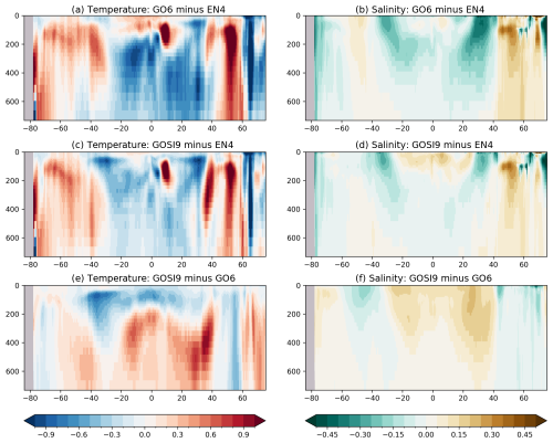
Figure 5 Zonal-mean potential temperature (K) and salinity: anomalies against 20-year climatology of EN4 v1.1 (Good et al., 2013) for the $\mathrm{1}/\mathrm{4}\mathit{°}$ configuration for GOSI9 and GO6 and differences between GOSI9 and GO6. Model fields are time means over the third decade of integration.

Both models exhibit a tendency to develop cold biases in the tropics and the Arctic and warm biases in the extra-tropics and Southern Ocean. The cold bias between 200 and 700 m present in GO6 between 30° S and 40° N is still present in GOSI9 but is significantly reduced, especially in the $\mathrm{1}/\mathrm{4}\mathit{°}$ resolution (Fig. 5). The near-surface warm bias in the tropics is also greatly reduced, and there is a modest reduction in the cold bias in the Arctic. There is a slight degradation in the Southern Hemisphere extra-tropics, with a cold bias developing near 30° S at 50–100 m depth and a slight increase in the warm bias between 40–60° S below 200 m. Salinity biases reduce at most latitudes and depths, although a modest positive salinity bias develops in the shallow subsurface tropics. Overall, GOSI9 shows reduced temperature and salinity biases at most latitudes and depths.

We can attribute these changes to each of the development steps by comparing the simulations for each of the intermediate steps (Table 3). Figure 6 shows the incremental temperature and salinity anomalies that arise from updating the NEMO code from v3.6 to v4.0 (a, b), increasing the global mean chlorophyll concentration value to 0.1 mg m⁻³ (c, d) and adjusting the nn_htau parameter that controls TKE mixing penetration (e, f). Upgrading to NEMO 4.0 results in a warming between 100 and 700 m between 20° S and 40° N and in the Arctic (Fig. 6a) and is the change primarily responsible for reducing the cold bias observed in GO6 in these regions (Fig. 5a). It also acts to increase the salinity in the shallow tropical region (Fig. 6b), partially compensating for the fresh biases in GO6 (Fig. 5b) and leading to the slight saline bias in GOSI9 (Fig. 5d). Increasing the chlorophyll concentration to 0.1 mg m⁻³ has a cooling effect, which reduces subsurface warm biases in the tropics but slightly increases cold biases in the extra-tropics (Fig. 6c). The increase in chlorophyll does not affect the salinity. Adjusting the nn_htau parameter cools the subsurface between 50 and 300 m and reduces the warm bias present in these layers between 30 and 40° S, but in the forced GOSI9 configuration it introduces a cold bias centred at 100 m. This change also has a negligible effect on salinity. Its isolated effect is presented in Fig. 6e and f. Despite the mixed impact on the forced GOSI9 configuration, the nn_htau adjustment was implemented with the purpose of keeping the same ocean configuration for forced and coupled applications. In the forced integration, GOSI9, the impact on the surface is more limited than in the coupled model as the SST is constrained by the bulk formulae, but the impact on the subsurface is significant.

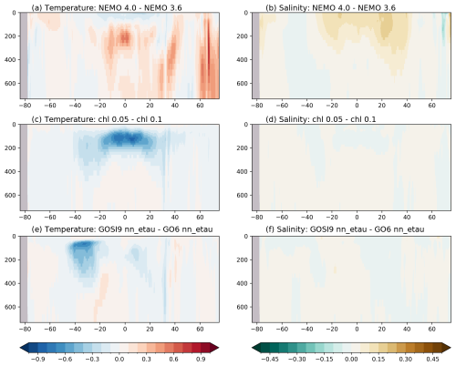
Figure 6 Zonal-mean potential temperature (K, a, c, e) and salinity (b, d, f) anomalies resulting from updating the NEMO code from v3.6 to v4.0 (a, b), increasing the global mean chlorophyll concentration value to 0.1 mg m⁻³ (c, d) and adjustment of the nn_etau parameter that controls TKE mixing penetration (e, f). Model fields are time means over the third decade of integration.

The more accurate tracer advection was found to result in reductions in the effective diffusivity, as defined by Megann (2018), of around 10 %, as well as robust improvements in model biases, which were mainly attributed to increasing the order of the horizontal advection. Figure 7 shows the impact of the fourth-order advection on the temperature in the top 700 m in the $\mathrm{1}/\mathrm{4}\mathit{°}$ configuration. Overall, using the fourth-order advection tends to warm the ocean, especially in the Atlantic basin. The impact is also seen on the western boundary currents (Gulf Stream and Kuroshio) where the steering is changed.

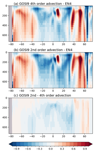
Figure 7 Potential temperature anomalies averaged over 0–700 m against the EN4 v1.1 average for 1995–2014 (Good et al., 2013) for GOSI9 and GOSI9 2nd order and difference between GOSI9 2nd order and GOSI9. Experiments GOSI9 and GOSI9 2nd order are detailed in Sect. 3 and Table 3. Model fields are time means over the third decade of the integrations.

4.2.2 Spatial biases

While the ability of a model to adequately represent globally or zonally integrated properties is important for applications such as climate projections and Earth system model studies, minimizing regional biases is also critical, not only for the regions in question but also for the climate and weather downstream. In this section we systematically assess the geographical distribution of biases.

For both GO6 and GOSI9, the three resolutions show a similar distribution of large-scale temperature and salinity biases. In GO6, temperatures are too warm at the surface and subsurface (Figs. 8 and 9) in the Southern Ocean, in the tropics and in the Arctic Ocean. Changes made in GOSI9 significantly reduce the biases in the Arctic, especially for the 1 and $\mathrm{1}/\mathrm{4}\mathit{°}$ resolutions. This improvement is linked to an improved representation of Arctic sea ice in GOSI9, especially in summer when the melting has been reduced and is in much better agreement with the observations. The warm SST bias in the tropics present in GO6 is reduced in GOSI9; however, the warm biases in the coastal upwellings in the eastern Pacific and eastern Atlantic are still present. At 100 m depth, GOSI9 is significantly cooler than GO6 (Figs. 9 and 5) as a result of the increased chlorophyll concentration. This change is net positive globally, reducing the warm bias centred at 100 m and present at all resolutions in GO6 (Fig. 5). However, it introduces regional cold biases, especially in the Indian Ocean. In the North Atlantic subpolar gyre, there is a dipole of cooling and warming, which is discussed in further detail in Sect. 5.2. Looking at the sea surface salinity, GO6 has large-scale fresh biases between 40° S and 40° N (Fig. 10). Outside the Arctic, the largest biases occur in the locations where subtropical mode waters ventilate. These subtropical surface fresh biases extend to depths of 500 m in the $\mathrm{1}/\mathrm{4}\mathit{°}$ and $\mathrm{1}/\mathrm{12}\mathit{°}$ resolutions (Fig. 5). With the upgrade to NEMO4 and its more accurate bulk formulae, these fresh biases are significantly reduced in GOSI9 and do not extend as deep (Fig. 5). In the Arctic, the fresh biases present in GO6 are reduced in GOSI9. We note that comparison with EN4 in the Arctic is problematic due to the existence of artificial spatial patterns arising from the interpolation of sparse observational data. Figures 11 and 12 show the annual minimum and maximum mixed-layer depth biases compared to de Boyer Montégut et al. (2004), respectively. Summer minimum mixed-layer depths are in good agreement with observations in all three models. There is an overall tendency towards a slight shallow bias on the order of 5–10 m, with deep biases at the Equator and in a few regions around the Southern Ocean. Storkey et al. (2018) noted that the winter mixed-layer is too deep in the North Atlantic subpolar gyre, in the Greenland–Iceland–Norway seas and in the Southern Ocean west of the Drake Passage. These biases are still present in GOSI9 but with reduced amplitude. For the 1° resolution, biases in the NE Atlantic change from positive to negative, while the strong bias in the Labrador Sea is almost eliminated. Apart from these regions, differences in mixed-layer depth between GO6 and GOSI9 can be observed in a latitudinal band around 40° S. This corresponds to the region where the TKE mixing depth has been reduced in GOSI9 (Sect. 2.5.8). Shallowing of mixed-layer depth between GOSI9 and GO6 at around 40° S and at around 60° N is more clearly visible in Fig. S2 in the Supplement, showing the mixed-layer depth zonal mean for both models.

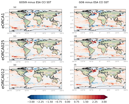
Figure 8 Sea surface temperature anomalies against the ESA CCI average for 1996–2014 (Merchant et al., 2014) for GOSI9 and differences between GOSI9 and GO6. Model fields are time means over the third decade of the integrations.

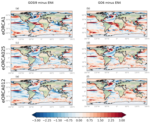
Figure 9 Potential temperature anomalies at 100 m against the EN4 v1.1 average for 1995–2014 (Good et al., 2013) for GOSI9 and differences between GOSI9 and GO6. Model fields are time means over the third decade of the integrations.

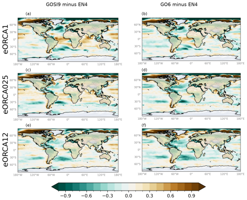
Figure 10 Sea surface salinity anomalies against the EN4 v1.1 average for 1995–2014 (Good et al., 2013) for GOSI9 and differences between GOSI9 and GO6. Model fields are time means over the third decade of the integrations.

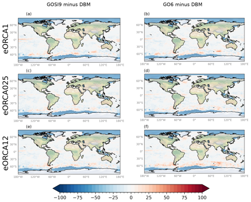
Figure 11 Annual minimum mixed-layer depth (in metres) anomalies against de Boyer Montégut et al. (2004) climatology for GOSI9 and GO6 and differences between GOSI9 and GO6. Model fields are time means over the third decade of integration.

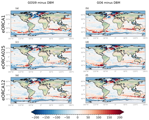
Figure 12 Annual maximum mixed-layer depth (metres) anomalies against de Boyer Montégut et al. (2004) climatology for GOSI9 and GO6 and differences between GOSI9 and GO6. Model fields are time means over the third decade of integration.

4.2.3 Sea ice

The seasonal cycle of sea ice area and volume is much improved in GOSI9 in both the Northern Hemisphere and Southern Hemisphere (Fig. 13). This represents a marked improvement over GO6, for which the Arctic summer minimum was significantly lower than observed, especially for the 1 and $\mathrm{1}/\mathrm{4}\mathit{°}$ resolutions. Ice representation is similar across the resolutions in GOSI9, and thus for conciseness we show only the assessment of $\mathrm{1}/\mathrm{4}\mathit{°}$. Given the change in ice model from CICE5 to SI³, it is difficult to attribute these improvements more precisely. However, one significant change is the increase in albedo (Sect. 2.5.2). Tested separately, it resulted in increased sea ice thickness and reduced melt in summer Arctic sea ice (not shown). This is consistent with work from Rae et al. (2014) that shows how sensitive the sea ice models are to parameter changes that affect the surface radiation and highlights that Arctic sea ice is the most sensitive to snow albedo. Figure 14a–c shows the September mean for Arctic sea ice concentration for the $\mathrm{1}/\mathrm{4}\mathit{°}$ configuration at GOSI9, gridded observations from HadISST, and the $\mathrm{1}/\mathrm{4}\mathit{°}$ configuration at GO6. The Northern Hemisphere distribution of sea ice in GOSI9 is in much better agreement with observations than GO6, though concentrations are still lower than observed over the central Arctic. Increasing the albedo in GOSI9 reduces the summer melt, allowing a better representation of the minimum sea ice area. As a result of improving the sea ice area in summer, the temperature and salinity biases are also reduced (Figs. 8 and 10). Sea ice distribution in the Southern Hemisphere is also improved (Fig. 14d–f), though concentrations close to Antarctica in the Weddell, Bellingshausen, Amundsen and Somov seas are all lower than observed. In the model, low concentrations of ice not present in the observations also extend east of the Weddell Sea into the Lazarev Sea.

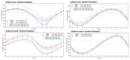
Figure 13 Mean seasonal cycles for integrated sea ice area (a, c) and sea ice volume (b, d) for the Northern Hemisphere and Southern Hemisphere for GOSI9 and GO6-GSI8.1 for eORCA025. The meaning period is 1995–2014. In the panels representing the sea ice area (a, c), HadISST analysis (Titchner and Rayner, 2014) is represented in grey. For the Northern Hemisphere volume (b) PIOMAS reanalysis (Zhang and Rothrock, 2003) is represented in grey. Dotted grey lines show mean ± σ, while dashed grey lines show the mean ±20 %.

Overall, GOSI9 exhibits a more consistent and realistic representation of sea ice across the different resolutions than GO6+GSI8, for which the $\mathrm{1}/\mathrm{12}\mathit{°}$ configuration was more realistic than the other two resolutions.

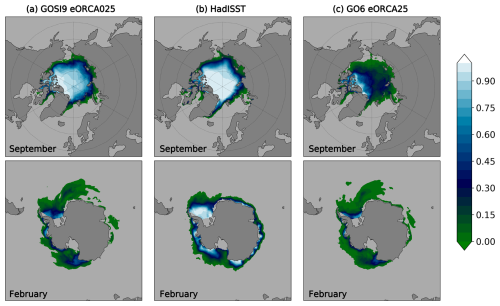
Figure 14 September mean for Arctic sea ice concentration (top) and February mean fort the Southern Ocean (bottom) averaged for 1995–2014 in GOSI9 eORCA025 (a), GO6-GSI8.1 eORCA025 (c) and HadISST (b) analysis (Titchner and Rayner, 2014).

5 Evaluation of model performance in specific regions of interest

Since GO6, concerns have been raised as to whether biases in specific regions of interest are limiting model performance, particularly in coupled forecasts and climate projections. In response, JMMP have established process evaluation groups (PEGs) with the remit of identifying the causes of biases and to advising on or delivering improvements to the model. To facilitate validations against observations and model comparison, key metrics have been identified and developed in a set of validation tools. These validation tools, MARINE_VAL, are available at https://github.com/JMMP-Group/MARINE_VAL (last access: 21 January 2025). In this section, we evaluate the improvements in model performance in three key regions.

5.1 The Southern Ocean and Antarctic Circumpolar Current

As described in Sect. 2.5.6, significant work has been done to try to reduce large-scale biases in the Southern Ocean in the coupled models with eddying ocean model resolution. In this section, we show the impact of these changes in the forced model. The coupled results will be described in detail in a separate publication, but here we also show results from a recent version of the HadGEM3 coupled model for illustration and comparison with the forced model results.

The biases are characterized by scalar metrics, as detailed in the caption of Fig. 15, in order to capture their time evolution. The immediate goal of the Southern Ocean package of changes in GOSI9 is to damp the overactive subpolar gyres in the Southern Ocean. The gyres in the Weddell Sea and Ross Sea are both too active at GO6 eddying resolutions and reduced in strength at GOSI9 (Fig. 15b and c). This change is primarily due to the Southern Ocean package, although the change to fourth-order advection in the horizontal also has a beneficial impact (not shown). The results for the coupled model (eddy-permitting ocean resolution, present-day forcing) show that the biases are larger than for the forced models due to coupled model feedbacks and are significantly reduced by the Southern Ocean package of changes.

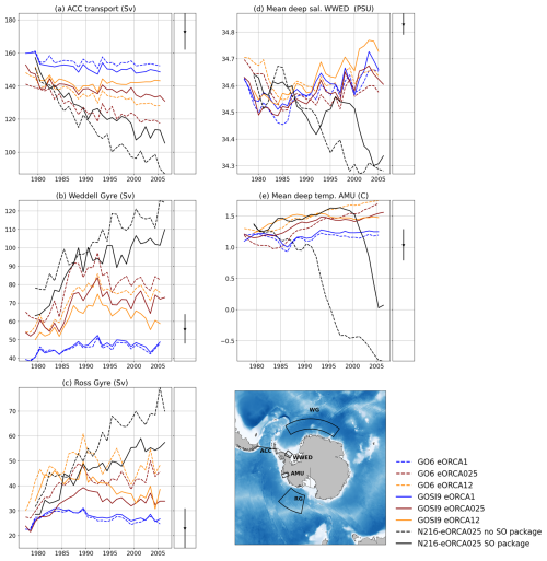
Figure 15 Time series of Southern Ocean metrics for the 30 years of GOSI9 and GO6 integrations compared with 30 years of a present-day forcing integration of two prototypes of the GC5 coupled model (N216-eORCA025) with and without the Southern Ocean Package described in Sect. 2.5.6. The plotted quantities are annual means. Observational estimates and uncertainties are plotted as the black dots and lines to the right of the time series plots. The panels show the following information: (a) the net eastward transport in the Drake Passage (cf. Donohue et al., 2016), (b) the transport of the Weddell gyre as indicated by the maximum streamfunction in the WG box (cf. Klatt et al., 2005), (c) the transport of the Ross gyre as indicated by the maximum streamfunction in the RG box (cf. Dotto et al., 2018), (d) the salinity below 400 m spatially averaged over the WWED box in the western Weddell Sea, and (e) the temperature below 400 m averaged over the AMU box in the Amundsen Sea. For (d) and (e), observational estimates are calculated from the EN4.2.2.g10 profile dataset (Good et al., 2013) using means and standard deviations for all the profiles with data below 400 m in the defined boxes.

The metrics for the subpolar gyre strengths are based on the local maximum of the barotropic streamfunction. By construction, this is the sum of the transport in the circumpolar Antarctic Slope Current (ASC) and the recirculating transport in the gyre. A large part of the reduction in this transport metric is due to a reduction in the strength of the ASC. This has the additional effect of reducing an unrealistically large westward flow at the southern boundary of the Drake Passage and hence increasing the net eastward transport in the Drake Passage (Fig. 15a). The GO6 models at all resolutions have net Drake Passage transport that is too small compared to the estimate of Donohue et al. (2016), with the largest bias being at eddy-permitting resolution. The biases are significantly reduced at GOSI9 for the eddying models. Again, the biases in the coupled eddy-permitting model are larger than in the equivalent forced model, and there is a similar reduction with the use of the Southern Ocean package.

The very strong ASC in the eddying models tends to act as a barrier to exchange of water and ice between the Antarctic shelf and the open ocean (as also noted by Beadling et al., 2022). This tends to lead to biases in the water mass properties on the shelves. Two examples are shown here. The deep shelf water in the western Weddell Sea tends to be too fresh in the coupled model integrations. This is a region of deep-water formation, and the freshening indicates that the process of deep-water formation is tending to shut down in the model. The Southern Ocean package reduces this bias to some extent. The forced models have a smaller fresh bias in this region, which is somewhat reduced at GOSI9 compared to GO6. The other example is in the Amundsen Sea where relatively warm and salty circumpolar deep water (CDW) impinges onto the shelf. In the coupled model at eddy-permitting resolution, the strong ASC acts as a barrier to this, and we see cold biases developing in this region, which are partially alleviated by the Southern Ocean package. In the forced models in this case we do not see the same biases. If anything the water in this region is slightly too warm, and there is little difference between GO6 and GOSI9.

5.2 The North Atlantic

The North Atlantic and its subpolar gyre is a key region for European weather and climate and is also where some of the largest biases on all three model resolutions occur. It is a dynamically active region where we see significant differences in ocean currents and temperature and salinity biases between the different resolutions. In the GO6 1° configuration, a strong cold bias in excess of −3 K manifests to the north of the Gulf Stream and east of Newfoundland (Fig. 8). All three resolutions exhibit a warm bias throughout the rest of the subpolar gyre, which is in excess of 3 K in the eastern lobe of the subpolar gyre. Changes introduced in GOSI9 have resulted in a substantial reduction in this warm bias at all three resolutions. The cold bias at 1° remains similar in extent and magnitude, and where the warm bias has been corrected a more muted version of this cold bias is also now present at $\mathrm{1}/\mathrm{4}\mathit{°}$. Strong SST gradients exist across the Gulf Stream separation and North Atlantic Current, meaning that biases of this magnitude can easily arise from biases in the position of the main current pathways in this region.

The Gulf Stream (GS) separation is known to be sensitive to resolution (Chassignet and Marshall, 2008; Marzocchi et al., 2015). Chassignet and Marshall (2008) states that a resolution on the order of at least $\mathrm{1}/\mathrm{10}$° is a necessary condition for a western boundary current to realistically separate from the coast. Figure 16f shows GS separation latitude for the three GOSI9 resolutions. The GS pathway is diagnosed using the 15 °C isotherm at 200 m following (Seidov et al., 2019), and the latitude of the GS at 72° W is displayed. In the 1° configuration, the GS separates too far north at 38.5° N and fails to deflect northwards. The position of the North Atlantic Current (NAC) is calculated with a method similar to the one used to diagnose the GS position but using the 10 °C isotherm at 50 m depth. The latitude of the NAC at 41° W is shown in Fig. 16g. In the 1° configuration the NAC position is 7° further south than observations. The poor representation of the GS and NAC in the 1° model was already highlighted in GO6 (Storkey et al., 2018) and is a known issue in eddy-parameterizing models (Zhang and Vallis, 2007). The lack of northward advection of warm and salty water from the GS results in fresh and cold biases off Newfoundland (Figs. 8, 9, 10a and 16c). In the $\mathrm{1}/\mathrm{4}\mathit{°}$ data, as in the 1° data, the GS separates too far to the north, but the position of the NAC is noticeably improved compared with the 1° data (Fig. 16g). At $\mathrm{1}/\mathrm{12}\mathit{°}$, the GS does not overshoot but separates further south than observations. The separation being too far from the coast in the $\mathrm{1}/\mathrm{12}\mathit{°}$ was already apparent in GO6 and in the coupled model based on GO6 (Grist et al., 2021). The pathway of the NAC in $\mathrm{1}/\mathrm{12}\mathit{°}$ is better represented than in the lower-resolution models and brings warmer and saltier water into the North Atlantic subpolar gyre (Figs. 8 and 10). Compared with GO6, there is no significant change in the GS separation latitude. However, GOSI9 exhibits a southward shift in the NAC compared with GO6. In GO6, the position of the NAC in $\mathrm{1}/\mathrm{4}\mathit{°}$ and $\mathrm{1}/\mathrm{12}\mathit{°}$ varies between 52 and 56° N (not shown), which further north than the observations. In GOSI9, the position of the NAC is in better agreement with observations and is mainly due to the impact of the fourth-order advection on the steering around Grand Banks (not shown). The additional GM poleward of 50° and the upgrade to NEMO4 also contribute to the southward shift but to a lesser extent (not shown). As a result of this southward shift in the NAC, the northward advection of heat and salt is reduced in GOSI9. It reduces the warm and salty bias present in the subpolar gyre in GO6 and highlighted in Treguier et al. (2005) and Marzocchi et al. (2015). Marzocchi et al. (2015) linked the warm and salty bias to the strength of the cyclonic subpolar gyre. However, the reduction in the temperature and salinity biases in GOSI9 is not associated with a change in the strength of the subpolar gyre (not shown).

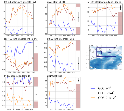
Figure 16 Time series of North Atlantic metrics for the 30 years of GOSI9 integrations. The plotted quantities are annual means. When available, observational estimates and uncertainties are plotted as the black dots and lines to the right of the time series plots. The panels show the following information: (a) subpolar gyre strength (Sv), (b) AMOC at 26.5° N at maximum depth (Sv) compared to 2004–2008 RAPID array (Moat et al., 2020), (c) mean sea surface temperature over the box off Newfoundland (°C), (d) mean mixed-layer depth in the Labrador Sea box (m) (cf. de Boyer Montégut et al., 2004), (e) mean sea surface salinity in the Labrador Sea box, (f) Gulf Stream separation latitude at 72° W (° N) calculated using the 15 °C isotherm at 200 m following Seidov et al. (2019), and (g) North Atlantic Current latitude at 41° W (° N) calculated using at 10 °C isotherm at 50 m depth following a similar method to that used for the Gulf Stream separation. For (c), (e), (f) and (g), observational estimates are calculated from EN4.2.2.g10 profile dataset (Good et al., 2013) using means and standard deviation.

The time series of the annual-mean AMOC at 26°5 N are shown in Fig. 16b. Observations from the RAPID array (Moat et al., 2020) between 2004–2018 estimate the transport to be 17.1 Sv with an estimated annual-mean rms uncertainty of 1.5 Sv. Transport estimates prior to RAPID suggest that the AMOC was slightly stronger during the 1980s and 1990s, with net transport from a 1992 hydrographic section calculated as 19.4 Sv (Bryden et al., 2005). Annual mean AMOC transports in the $\mathrm{1}/\mathrm{4}\mathit{°}$ and $\mathrm{1}/\mathrm{12}\mathit{°}$ GO6 models were unrealistic (Storkey et al., 2018), peaking at 26 and 29 Sv, respectively, in the mid 1990s. Values in 2005 remained outside of observations, at 21 and 23 Sv. In contrast, the 1° model showed excellent agreement with observations, with a peak transport of around 20 Sv in the mid to late 1990s, reducing to 17 Sv in 2005. Improvements in GOSI9 have reduced the AMOC in the $\mathrm{1}/\mathrm{4}$ and $\mathrm{1}/\mathrm{12}\mathit{°}$ models so that both now peak at 20–21 Sv in 1995 and reduce to values around 17 Sv in 2005. The reduction in AMOC is associated with a decrease in the deep bias in the subpolar gyre and GIN seas mixed-layer depth (Fig. 12). However, the convective overturning in the Labrador Sea is still too high in both the $\mathrm{1}/\mathrm{4}\mathit{°}$ and $\mathrm{1}/\mathrm{12}\mathit{°}$ configurations (Fig. 16d). This suggests that the AMOC at the $\mathrm{1}/\mathrm{4}$ and $\mathrm{1}/\mathrm{12}\mathit{°}$ models is driven too much by excessive deep mixing in the Labrador Sea, as previously noted by Megann et al. (2014). The excessive deep convection in the Labrador Sea (Fig. 16d) is common in numerical ocean models (Courtois et al., 2017). Chanut et al. (2008) highlights the crucial role played by eddies in the re-stratification process, but even at $\mathrm{1}/\mathrm{12}\mathit{°}$ these eddies are not fully resolved. Unfortunately, AMOC volume transport in the 1° model is now too weak, around 16 Sv in 1995 and 13–14 Sv in 2005. Sensitivity experiments were carried out with the 1° model to understand the changes in AMOC strength from GO6 to GOSI9, and the changes in AMOC are mainly driven by the increased albedos in GOSI9 and the improved the sea ice cover (not shown). We speculate that in GO6 the 1° model may have been getting the right answer for the wrong reason, with the unrealistically low sea ice coverage in late summer–early winter exposing the surface of the ocean and leading to strong heat loss, strong deep convection and a more vigorous AMOC. There is less than 2 years of overlap between the RAPID observation-based estimates of the strength of the AMOC and the reference simulations. This will be addressed in the next development cycle, for which we will update the forcing product used. It is also worth noting that the strength of the AMOC in numerical simulations is known to be sensitive to both the choice of forcing product and the strength of numerical mixing at tropical and subtropical latitudes (e.g. Megann and Storkey, 2021), meaning that care should be taken not to try to overfit transport in forced ocean models to the observations.

5.3 The northwestern Pacific

The Kuroshio is the western boundary current in the northern Pacific subtropical gyre and plays an important role in transporting heat poleward. Following methods described in Qiu et al. (2014) and Qiu and Chen (2005), the position and strength of the Kuroshio is calculated for the 30-year GOSI9 integrations at all resolutions and compared with sea surface height observations from CMEMS for the period 1994–2006 (https://doi.org/10.48670/moi-00149, Copernicus Marine Service, 2024). The position of the Kuroshio extension in the 1° configuration (38° N) and in the $\mathrm{1}/\mathrm{4}\mathit{°}$ configuration (37° N) is further north than in the observations (35° N), while the $\mathrm{1}/\mathrm{12}\mathit{°}$ configuration is in better agreement with the observations (Fig. 17a). An et al. (2023) shows that coupled models with eddy-rich ocean models better depict the Kuroshio extension dynamic and thermal structure than models with lower-resolution ocean data. Guo et al. (2003) show that as the resolution increases, the path, intensity and vertical structure of the Kuroshio improves. They observed a northwards overshoot with the lower-resolution model. They highlight that with increased resolution, the better representation of topography results in better reproduction of the interaction between baroclinicity and bottom topography. In addition to a better representation of the position of the Kuroshio extension, in the $\mathrm{1}/\mathrm{12}\mathit{°}$ configuration the intensity of the current is in better agreement with the observations than in the 1° and $\mathrm{1}/\mathrm{4}\mathit{°}$ configurations (Fig. 17b). It is noted that the intensity of the Kuroshio is very weak compared to the observations in the 1° configuration. The subarctic frontal zone formed by the convergence of cold water from the Oyashio and warm water from the Kuroshio is shifted northward in the two lower-resolution models, and this results in a warm anomaly (Fig. 9).

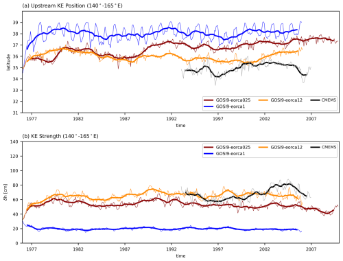
Figure 17 Time series of Kuroshio metrics for the 30 years of GOSI9 integrations and for the 13 years of observations from the altimeter satellite-gridded sea level anomalies (EU Copernicus Marine Service Information (CMEMS), Marine Data Store (MDS), https://doi.org/10.48670/moi-00149, Copernicus Marine Service, 2024). Annual (thick lines) and monthly (thin lines) data are plotted. (a) Kuroshio extension zonal-averaged latitude position in 140–165° E calculated following Qiu et al. (2014); Qiu and Chen (2005). (b) Kuroshio extension strength calculated using the sea surface height difference across the Kuroshio extension as in Qiu et al. (2014).

6 Summary and discussions

GOSI9 is the latest UK global ocean and sea ice configuration developed by the JMMP partnership (Met Office, National Oceanography Centre, British Antarctic Survey, and Centre for Polar Observation and Modelling), superseding GO6 (Storkey et al., 2018). GOSI9 is a traceable hierarchy of three horizontal resolutions, i.e. 1, $\mathrm{1}/\mathrm{4}$ and $\mathrm{1}/\mathrm{12}\mathit{°}$, and is based on the NEMO version 4.0.4 code (Madec and NEMO system team, 2019). The upgrade to NEMO 4.0.4 includes a new sea ice model SI³ (Sea Ice modelling Integrated Initiative) and faster integration achieved through the use of partially implicit schemes that allow a significant increase in the length of the time step. Other developments include the upgrade to the TEOS10 equation of state, a reduction in numerical mixing, and improved representation of the Southern Ocean. The interactive icebergs used in GO6 (Bigg et al., 1997; Martin and Adcroft, 2010) are switched off in GOSI9 due to stability issues, especially while testing with the coupled model. It is replaced by an iceberg melt climatology. The impact of these changes, principally in the $\mathrm{1}/\mathrm{4}\mathit{°}$ model, are presented. The upgrade to NEMO 4.0.4 has a large impact, with a significant reduction in the temperature and salinity biases (Figs. 3b and 4b). Adopting the fourth-order horizontal and vertical advection reduces the numerical mixing, helping to minimize the cold bias developing below 200 m (Fig. 3c and f). While the changes introduced to improve the representation of the Southern Ocean in the $\mathrm{1}/\mathrm{4}$ and $\mathrm{1}/\mathrm{12}\mathit{°}$ configurations have limited impact on the warm SST bias in the forced model, they result in a stronger and more realistic ACC transport and a reduction in the temperature and salinity biases along the shelf of Antarctica (Fig. 15).

Tests with the coupled model were carried out in the early phase of GOSI9 development. This allowed us to integrate further tuning required for the coupled model early during the development cycle. In particular, after testing with the coupled model, changes in TKE mixing depth and increased chlorophyll concentration were introduced to reduce subsurface biases. These two changes have a positive impact on both forced and coupled models.

The results from the 30-year integrations forced by the CORE2 dataset are presented for the three resolutions and compared against the GO6 integrations. In GOSI9, significant reductions in temperature and salinity drifts from initial condition are realized. Below 200 m these are mainly due to the upgrade to NEMO 4.0.4 and fourth-order advection, and in the top 200 m they are primarily a result of the change in chlorophyll (Fig. 3). The global warm SST bias is reduced in the tropics and Arctic, while minimal changes are observed in the Southern Ocean. Large improvements in Arctic surface temperature and salinity are linked to the improved sea ice representation. In particular, the excessive and unrealistic Arctic summer sea ice melt in GO6 is significantly improved in GOSI9 (Fig. 14) and can be attributed to the change in the sea ice model to SI³ and to the higher albedos that increased sea ice thickness.

The next round of development will focus on improving model fidelity in the North Atlantic and will include work already carried out to improve the representation of the Nordic overflows. Bruciaferri et al. (2024) combined the idea of Colombo (2018) with the multi-envelope approach of Bruciaferri et al. (2018) to successfully implement localized terrain following coordinates in the Nordic overflow region. Their generalized approach has been tested with the GOSI9 $\mathrm{1}/\mathrm{4}\mathit{°}$ configuration and is shown to significantly improve the realism of the Nordic overflows in simulations, reducing spurious cross-isopycnal mixing in this region of strong gravity currents. However, large-scale salinity biases along the bathymetry of the subpolar gyre impact the mass properties of the water cascading. Improving the salinity bias and using appropriate coordinates are both key to improving the representation of the Nordic overflows. Another key challenge is to realistically represent the separation latitude of the Gulf Stream. In the GOSI9 configuration, increasing the resolution is shown to improve the realism of the Gulf Stream separation latitude and the North Atlantic Current path. However, even with the $\mathrm{1}/\mathrm{12}\mathit{°}$ configuration this remains challenging. Work looking at the sensitivity of the Gulf Stream to the vertical coordinate system is ongoing (Bruciaferri et al., 2022), with the same approach being used for the Nordic overflows, and in parallel we plan to develop a $\mathrm{1}/\mathrm{12}\mathit{°}$ configuration with a two-way-nested Adaptive Grid Refinement In Fortran (AGRIF) zoom with a $\mathrm{1}/\mathrm{36}\mathit{°}$ configuration in the North Atlantic.

In GOSI9, progress have been made in the Southern Ocean with increased ACC transport and reduced temperature and salinity biases on the Antarctic shelf, but ice–shelf cavities have remained parameterized. For climate applications requiring open ice cavities, such as the UK Earth System Model (UKESM) configurations (Smith et al., 2021), improving water mass properties on the shelf is essential. Using a 1° forced configuration, Hutchinson et al. (2023) show that explicitly simulating the circulation beneath the largest ice shelves improves the realism of the Antarctic continental shelf circulation. However, they note that the impact on the representation of the Antarctic Bottom Water is limited by the absence of realistic overflows. Recent work under the NERC-funded ORCHESTRA project showed the merits of using a vertical sigma coordinate around the Antarctic shelf region to greatly reduce temperature and salinity biases on the shelf and to preserve the density of Antarctic bottom water (Meijers et al., 2023). For the next configuration, we plan to open the ice shelf cavities, taking advantage of the developments available at NEMO 4.2, and adopt the strategy used in the Nordic overflows using local terrain following coordinates to improve the Antarctic overflows.

In GOSI9, the bathymetries for each configuration originate from a different source (see Sect. 2.1). In this respect, the hierarchy of resolutions is not fully traceable. For future GOSI configurations, work is ongoing to produce traceable bathymetry for each resolution.

In GOSI9, the constant value used for the chlorophyll concentration was tuned to better match climatological values in the tropics. For future configurations, the constant value will be replaced by a monthly chlorophyll concentration climatology derived from ocean colour observations that will better account for the variation in the solar penetration due to the large spatial and seasonal variability. For the coupled model, it will allow a consistent approach between the ocean models and the atmosphere models, where a varying chlorophyll concentration is already used to compute the albedo.

The vertical mixing closure schemes currently available in NEMO underestimate the impact of important sources of mixing, such as Langmuir turbulence and maximum turbulence due to shear at the base of the mixed layer. These sources of mixing are important for near-surface mixing globally (Belcher et al., 2012). As part of the UK OSMOSIS project, a more physically based mixing scheme has been developed and is being implemented in NEMO. We expect this will replace the existing TKE scheme in the next configuration.