GREAT v1.0: Global Real-time Early Assessment of Tsunamis

We introduce a tsunami warning technology towards a global real-time analysis. The technology is based on the analysis of acoustic signals generated together with the tsunami, due to the compression of the water layer. The acoustic signals propagate much faster than the tsunami and thus can be recorded at hydrophone stations, which in turn enables the analysis in real time. The presented technology comprises a collection of models that have been integrated into a software with the goal to make it operational and to complement efforts by warning centres and provide a more reliable assessment, globally. The main models that were integrated into the software are presented and briefly discussed. Test cases performed by the software are compared with DART buoy observations, showing satisfactory agreement, though discrepancies arise in particular at far distances and locations separated by land. The calculation time of a full global-scale analysis is in the order of tens of seconds on a standard multi-core machine, without reliance on pre-computations, making it an appropriate real-time forecast.

1 Introduction

Tsunamis pose a significant threat to coastal communities around the world, necessitating the development of effective early warning systems. The inception of tsunami warning systems can be traced back to the 1940s when Japan and the USA adopted earthquake-centric approaches, utilizing seismic data and applying empirical formulae for wave height, along with a shallow water assumption for travel time. Challenges persisted, marked by numerous false alarms, inadequate coastal risk assessment, and delayed warnings. Consequently, a significant shift occurred post-2004 towards global, tsunami-centric systems, incorporating advanced methodologies such as pre-computed scenarios, empirical formulae, and tide gauge observations to enhance accuracy. The 2004 Indian Ocean tsunami served as a catalyst for a global response, instigating a paradigm shift in worldwide tsunami hazard reduction. This transformation involved integrating real-time tsunami observations and sharing advancements on a global scale. The UN-coordinated global system underwent expansion, introducing regional warning centres and standardized procedures. Since the 1940s, tsunami warning technology has evolved with the establishment of extensive seismic networks, deployment of DART buoys, cabled observatories, and GPS buoys, providing real-time data. Advances in numerical models, coupled with high-performance computing (HPC), contributed to a more effective warning system with reduced false alarms (Tsuchiya and Shuto, 1995; Igarashi et al., 2011; Bernard and Titov, 2015; Kong et al., 2015). However, conventional tsunami warning systems still struggle with significant challenges, resulting in a high incidence of false alarms and unreliability. Igarashi et al. (2011) point out operational weaknesses in providing timely warnings for local tsunamis, especially in regions where the existing system relies on tsunami measurements, leaving insufficient time for warnings when the source and destinations are in proximity. The dependence on earthquake information often leads to precautionary alerts, later cancelled when sea level data indicate non-destructive waves. While this cautious approach prioritizes safety, it unintentionally undermines the credibility of tsunami warning centres (TWCs) and fosters public scepticism, with people viewing alerts as frequent false alarms. Since the 1950s, a substantial 75 % of tsunami warnings that prompted evacuations have turned out to be false, as illustrated by the economic losses exceeding USD 30 million during the evacuation of Honolulu in 1986. Addressing these issues necessitates enhancing detection capabilities and public awareness to mitigate the credibility and economic challenges associated with false alarms.

This paper presents a methodology integrated into a piece of software which is currently under development for operational purposes. In particular, the software is designed to enhance real-time early tsunami warning technology, integrating precursor signal detection, computational techniques, and deep-water tsunami detection. By employing cutting-edge mathematical and artificial intelligence (AI) models, the software analyses sound signals to assess tsunamis as they occur (currently virtually). The methodology integrates data from various measurement sources and allows for the real-time mapping of risk areas, including relevant travel paths, once the epicentre location is identified. By utilizing a machine learning model, the earthquake magnitude is calculated, and the mode of strike is classified, in order to determine whether the earthquake is tsunamigenic or not. The earthquake fault angle, or dip, may be horizontal, vertical, or at an arbitrary angle. Faults are categorized by their slip direction: dip-slip faults move along the dip plane, strike-slip faults move horizontally, and oblique-slip faults display both motions. Tsunamigenic earthquakes usually involve motion normal to the surface. The strike mode is defined as either horizontal (less likely to cause tsunamis) or vertical (most likely to cause tsunamis); see Gomez and Kadri (2021). Additionally, in cases where the mode of strike exhibits a vertical element, an inverse problem model is employed to calculate the probability density function of the fault's geometry and dynamics. These properties are then used in a direct model to determine the tsunami amplitude in each risk area. Notably, the computational time required for analysing a given acoustic segment is below 30 s on a standard multicore PC station.

Furthermore, the methodology has been successfully validated through testing on previous earthquakes that resulted in tsunamis (or in false alarms). Further enhancement to the machine learning model and the incorporation of more mechanisms for tsunami generation, such as due to landslides or volcanic eruptions, including meteotsunamis (Omira et al., 2022), can be implemented as well. The future deployment of this technology in leading warning centres is expected to significantly reduce false alarms and the associated costs, ultimately promoting the goals of inclusive, safe, resilient, and sustainable cities, as outlined in SDG Goal 11 of the UNESCO (see https://sdgs.un.org/goals/goal11, last access: 17 April 2024), and increasing the number of local Disaster Risk Reduction strategies, which is Target 5 of the Sendai Framework.

2 Scientific background

In this work, a methodology for a rapid tsunami warning system is presented. The methodology allows input data from various measurement sources and integrates existing analysis techniques. In particular, the methodology allows real-time mapping of risk areas of interest including relevant travel paths once the epicentre location is identified. Then live acoustic signals are analysed using machine learning to classify the earthquake magnitude and mode of strike (Gomez and Kadri, 2021). If the mode of strike has a vertical element, then an inverse problem model (Kadri et al., 2017; Mei and Kadri, 2018; Gomez and Kadri, 2023) can be employed to calculate the probability density function of the geometry and dynamics of the fault. These properties are fed back into a direct model (Mei and Kadri, 2018; Williams et al., 2021) to obtain the tsunami amplitude at each risk area. The CPU time required for analysing a given acoustic segment ranges from seconds up to a few minutes on a standard multi-core PC station. The methodology has been successfully tested on previous earthquakes that resulted in tsunamis (Gomez and Kadri, 2023). This section provides a brief scientific background on the key models employed in the proposed technology.

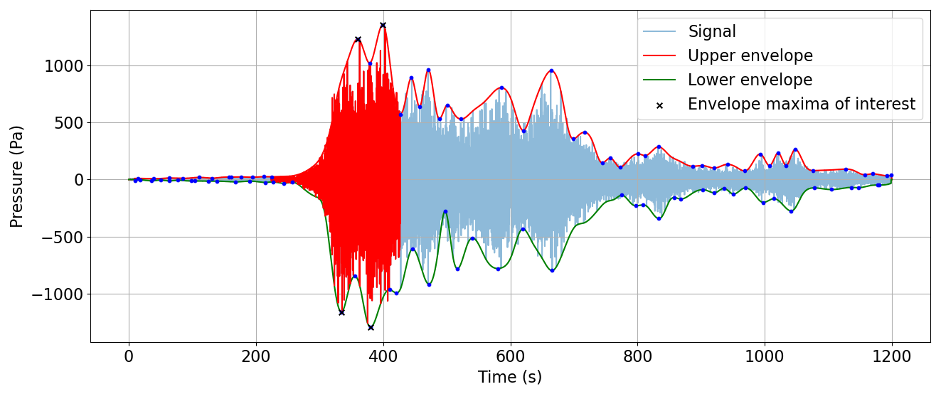
Figure 1 Test case 2004 M_w 9.1 Sumatra earthquake and tsunami. Analysed pressure signal. The signal was recorded at CTBTO's hydroacoustic station at Diego Garcia, H08S1. The analysis has been done automatically by the software for the region highlighted in red. The green and red curves are the lower and higher envelopes. This plot was created by the developed software GREAT.

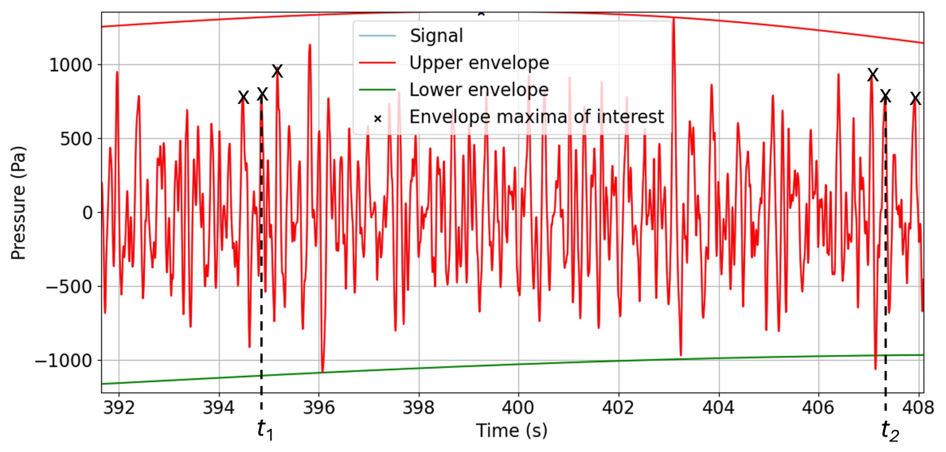
Figure 2 Test case 2004 M_w 9.1 Sumatra earthquake and tsunami. Enlarged view of the analysed pressure signal segment. The signal was recorded at CTBTO's hydroacoustic station at Diego Garcia, H08S1. The times are chosen at the peaks: t₁=407.03 s, t₂=394.83 s. The frequencies are calculated about each peak: ${\mathrm{\Omega }}_{\mathrm{1}}=\mathrm{2}\mathit{\pi }/\mathrm{0.35}$, ${\mathrm{\Omega }}_{\mathrm{2}}=\mathrm{2}\mathit{\pi }/\mathrm{0.7}$; c_l=1500 m s⁻¹. The depth at the hydrophone location h=1889 m. The green and red curves are the lower and higher envelopes. This plot was created by the developed software GREAT.

2.1 Hotspot model: Dijkstra's algorithm

The travel time is calculated on a triangular unstructured mesh with either global or regional coverage in the spherical coordinate system. The mesh files include ocean depth and Lame's elasticity constants λ, μ, and the earth density ρ_s. These data are used to calculate the phase speed of surface gravity waves (tsunamis), acoustic modes in the water body, and pressure-wave¹ and shear-wave² velocities (c_p and c_s) in the solid earth. The mesh file includes the node ID, coordinates (longitude and latitude), aforementioned variables, and the triangulation connectivity tables. The mesh can have uniform or spatially variable resolutions depending on the wave type. For P and S waves, a uniform mesh is adequate, while depth variable resolution is needed for acoustic and gravity waves. The hotspot model calculates the propagation speed of P, S, acoustic waves, and surface gravity waves based on the following procedure:

• P and S waves. The spatially variable speed of compressional c_p and shear c_s waves at the earth surface is related to Lame's elasticity constants λ and μ, and the earth density ρ_s. Lame's constants are taken from the PREM (Dziewonski and Anderson, 1981), and the anisotropic variability in the spherical coordinate system (latitude, longitude) is taken from Panning et al. (2010):

  $$\begin{array}{}\text{(1)}& c_p=\sqrt{{\displaystyle \frac{\mathit{\lambda }+\mathrm{2}\mathit{\mu }}{{\mathit{\rho }}_{\mathrm{s}}}}},c_{\mathrm{s}}=\sqrt{{\displaystyle \frac{\mathit{\mu }}{{\mathit{\rho }}_{\mathrm{s}}}}}.\end{array}$$

  The anisotropic, depth-dependent c_p and c_s values are subsequently interpolated onto a three-dimensional mesh. This configuration permits P waves to propagate through the mantle, outer, and inner core, whereas S waves are unable to penetrate the outer core.

• Acoustic waves. The phase speed and group velocity are calculated from the solution of the following dispersion relation for acoustic waves, which accounts for water compressibility and gravitational terms, neglecting the role of earth elasticity,

  $$\begin{array}{}\text{(2)}& \begin{array}{rl}& {\mathit{\omega }}^{\mathrm{2}}[\mathrm{1}-({\mathit{\gamma }}_l/\left(\mathrm{2}r\right)\left)\tanh rh\right]=gr(\mathrm{1}-({\mathit{\gamma }}_l/\left(\mathrm{2}r\right){)}^{\mathrm{2}})\\ & \tanh rh,\end{array}\end{array}$$

  with

  $$\begin{array}{}\text{(3)}& r^{\mathrm{2}}=k^{\mathrm{2}}-{\mathit{\omega }}^{\mathrm{2}}/c_l^{\mathrm{2}}+{\mathit{\gamma }}^{\mathrm{2}}/\mathrm{2},{\mathit{\gamma }}_l=g/c_l^{\mathrm{2}},\end{array}$$

  where r is the eigenvalue, k is the wavenumber, c_l is the sound speed in water, and g is the gravitational acceleration constant. The imaginary roots of Eq. (2) describe both progressive and spatially decaying acoustic wave modes, which are generated in a compressible fluid together with surface gravity waves (Abdolali and Kirby, 2017).

• Surface gravity waves. Considering the water compressibility, overlying a half-space elastic bed with gravitational terms, the dispersion relation is written as (Abdolali et al., 2019)

  $$\begin{array}{}\text{(4)}& \tanh \left(rh\right)={\displaystyle \frac{\left(C_{\mathrm{2}}+C_{\mathrm{3}}/g\right){\mathit{\omega }}^{\mathrm{2}}/r}{C_{\mathrm{1}}{C}_{\mathrm{2}}{\mathit{\omega }}^{\mathrm{2}}/r+C_{\mathrm{3}}\left(\mathrm{1}+{\mathit{\gamma }}_l{C}_{\mathrm{1}}/r\right)}},\end{array}$$

  where C₁, C₂, and C₃ are coefficients defined in Appendix A, and q and s are the eigenvalues:

  $$\begin{array}{}\text{(5)}& q^{\mathrm{2}}=k^{\mathrm{2}}-{\mathit{\omega }}^{\mathrm{2}}/c_p^{\mathrm{2}}+{{\mathit{\gamma }}_p}^{\mathrm{2}}/\mathrm{2},s^{\mathrm{2}}=k^{\mathrm{2}}-{\mathit{\omega }}^{\mathrm{2}}/c_{\mathrm{s}}^{\mathrm{2}}+{{\mathit{\gamma }}_{\mathrm{s}}}^{\mathrm{2}}/\mathrm{2},\end{array}$$

  where ${\mathit{\gamma }}_q=g/c_p^{\mathrm{2}}$ and ${\mathit{\gamma }}_{\mathrm{s}}=g/c_{\mathrm{s}}^{\mathrm{2}}$. The real root of the dispersion relation is used to calculate the phase speed and group velocity of tsunami waves.

At the initiation step of the hotspot model and per wave type, the nearest node in the mesh to the earthquake epicentre is identified. The weight for the elements' edges is calculated based on the Haversine formula and the phase speed of a given wave type between the nodes, as described earlier. In the second step, Dijkstra's algorithm (Dijkstra, 2022) is used to calculate the shortest path between the epicentre and all the nodes on the mesh (see Appendix B for more details).

The implemented model takes tens of seconds on a global unstructured mesh with 5–50 km resolution on a standard desktop machine and can do the simulations in parallel with other components of the system. The outputs of the model are the arrival time for the aforementioned waves and the transects from the source to all the nodes.

2.2 Machine learning: earthquake source inversion from acoustic signals

The machine learning model was originally developed by Gomez and Kadri (2021). They applied a range of techniques to analyse acoustic pressure signals generated by underwater earthquakes and calculate the effective fault size and dynamics in nearly real time. They used a dataset consisting of 201 earthquake signals recorded by the IMS hydroacoustic network and used 10 % of the data for validation and 10 % for testing. In addition, they used artificial data for further testing. The study compared four different methodologies for extracting relevant features from these acoustic signals, including statistical moments, time series analysis, power spectrum analysis, and wavelet transform coefficients analysis. Additionally, they employed two classification machine learning algorithms, random forest classifier (RFC) and support vector machine (SVM), to distinguish between vertical motion events and achieved over 70 % classification accuracy. Among these methodologies, the combination of wavelet transform feature extraction and SVM yielded the highest accuracy for both binary and multi-class scenarios.

Figure 3 The design of the software GUI.

Furthermore, the study applied regression machine learning algorithms to estimate the magnitudes of the tectonic events from the vectorized signals dataset. The machine learning algorithms provided more accurate predictions than simply using the mean value of the dataset, as confirmed by the sum of squared error (SSE) values. Notably, these algorithms, when combined with the precomputed vectorized dataset, took less than 1 s on a standard desktop machine to estimate the source magnitude and slip type. These estimates can be used as input for an inverse problem model to calculate the fault's effective size and dynamics in real time. The study, however, only considered shallow earthquakes to reduce uncertainties, and the depth dependence of classification accuracy remains unanalysed, a potential area for future research.

2.3 Direct model: pressure field and water amplitude calculations

The main objective of the direct model is to provide analytical calculations of the tsunami amplitudes at all regions of interest. Additionally, the model can calculate the pressure field induced by the acoustic waves, at any point of interest, but particularly at the hydrophone location, which allows a direct comparison against observations.

The model is based on an approach that was proposed by Mei and Kadri (2018), who considered the fault rupture to be slender and invoked multiple-scale analysis to obtain a closed-form analytical solution for the propagating acoustic modes. The earthquake fault is assumed to have a rectangular slender shape, characterized by a length of 2L and a width of 2b, where the slenderness parameter $\mathit{ϵ}=b/L\ll \mathrm{1}$. Due to this slender body assumption, Mei and Kadri (2018) were able to apply multiple-scale theory, introducing multiple-scale coordinates, $x,z,X={\mathit{ϵ}}^{\mathrm{2}}x,Y=\mathit{ϵ}y$, to derive a three-dimensional analytical solution of the pressure field (see Eq. 6.13 in Mei and Kadri, 2018). The closed form of the solution makes it ideal for real-time analysis. For example, the pressure field induced by the leading acoustic mode in the far field takes the form (see Eq. 8.5 in Mei and Kadri, 2018)

$$\begin{array}{}\text{(6)}& p={\mathit{\rho }}_l{W}_{\mathrm{0}}\left|A\right|{\displaystyle \frac{{\mathrm{2}}^{\mathrm{7}/\mathrm{2}}{c}_l}{\sqrt{{\mathit{\pi }}^{\mathrm{3}}{x}_{\mathrm{0}}k}}}\sin \left(kb\right)\sin \left(\mathrm{\Omega }T\right),\end{array}$$

where ρ_l is the water density, W₀ is the average uplift velocity of the fault, $A=A(k,X,Y)$ is the two dimensional envelope generated in the far field (defined in Appendix C), x₀ is the distance of the horizontal components at the observation point (e.g. hydrophone), k is the wave number, Ω is the frequency, and T is the duration of the effective uplift. Note that only the pressure induced by the first acoustic mode is considered here, as it carries most of the energy and information about the source (Mei and Kadri, 2018).

The solution by Mei and Kadri (2018) was modified later by Williams et al. (2021), who included the effects of gravity along with multi-faults. While to first order the acoustic modes are governed by compressibility of water, and surface gravity waves are governed by gravity, considering both gravity and compressibility (as well as elasticity effects) enhances the accuracy of the tsunami phase speed, as also shown by Abdolali et al. (2019). Similarly, including gravity modifies the dispersion relation of the acoustic modes, though in addition, it provides a closed-form solution for the generated tsunami. Thus, both the tsunami and the acoustic waves can be calculated simultaneously, which enhances the real-time analysis. The envelope of the surface elevation takes the form

$$\begin{array}{}\text{(7)}& \begin{array}{rl}\mathit{\eta }\left(x,y,t\right)& ={\displaystyle \frac{W_{\mathrm{0}}}{g\mathit{\pi }}}\left|A\right|{\displaystyle \frac{\mathrm{8}r\sin \left(kb\right)\sin \left(\mathrm{\Omega }T\right)\cosh \left(rh\right)}{k^{\mathrm{2}}\left[\mathrm{2}rh+\sinh \left(\mathrm{2}rh\right)\right]}}\\ & \sqrt{{\displaystyle \frac{\mathrm{2}\mathit{\pi }/t}{{\mathrm{\Gamma }}^{\prime \prime }\left(\mathrm{\Omega }\right)}}},\end{array}\end{array}$$

where Γ^′′(Ω) is given in Appendix D. Thus, given the basic properties of the fault, the tsunami can be calculated in the far field at extremely low computational cost.

Table 1 Sumatra 2004 tsunami height comparison between observations reported by Lay et al. (2005) and current model.

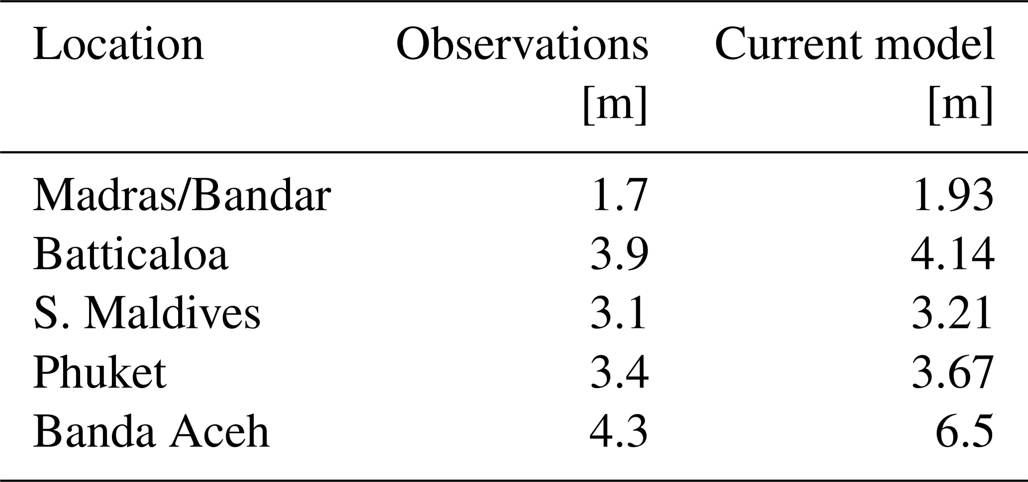
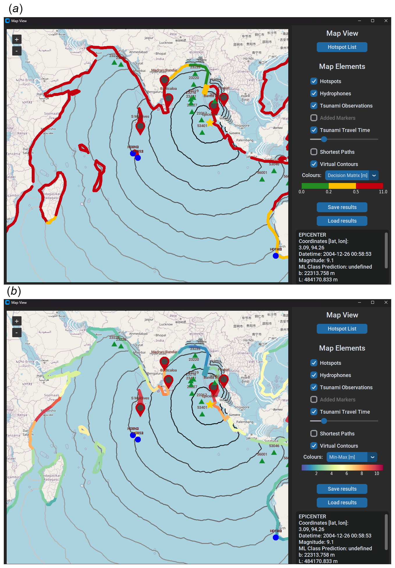
Figure 4 Screenshots of the software (GREAT) for test case 2004 M_w 9.1 Sumatra earthquake and tsunami. Yellow star: earthquake epicentre. Green triangles: the location of current DART buoys. Blue circles: hydrophone stations H08S and H08N. Hotspots: user-defined points of interest (red for high risk, yellow for middle risk). (a) A snapshot from the software for showing tsunami arrival times (black contours) and size (coloured contours) at 50 m depth. (b) A snapshot from the software for showing tsunami evaluation contours at the coasts (red for high risk, yellow for middle risk/advisory, and green for no risk) at 50 m depth. © OpenStreetMap contributors 2023. Distributed under the Open Data Commons Open Database License (ODbL) v1.0.

2.4 Inverse problem: calculating fault properties from acoustic data

The inverse problem approach of Hendin and Stiassnie (2013), originally devised for a circular fault, has been extended by Mei and Kadri (2018) to partially retrieve the main properties of a slender fault. Following that, a semi-analytical inverse problem approach has been developed by Gomez and Kadri (2021) to estimate the geometry, dynamics, and orientation of the fault by analysing real pressure signals recorded on the Comprehensive Nuclear-Test-Ban Treaty Organization (CTBTO) hydrophones. This approach allows for real-time calculation of the effective fault properties required in order to calculate the tsunami size. It is important to note that the geometry and dynamics of the slender fault represent an effective vertical motion, simplifying the more complex earthquake rupture dynamics. The ocean floor is assumed to move vertically at a constant speed.

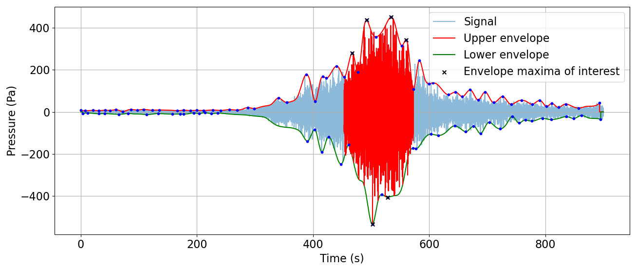
Figure 5 Test case 2011 M_w 9.1 Tohoku earthquake. Analysed pressure signal. The signal was recorded at CTBTO's hydroacoustic station at Wake Island, H11N. The analysis has been done automatically by the software for the region highlighted in red. The green and red curves are the lower and higher envelopes. The plot was created by the software GREAT.

The epicentre location and eruption time are usually known from seismic measurements, well before the acoustic data are available, and thus used as input parameters in the direct model. Nevertheless, an approximate calculation of the effective fault distance (x₀,y₀) and orientation can be made, for validation purposes, by the inverse problem model. However, the hydrophone station has to be sufficiently close, say within O(1000) km, so that the assumption of a Cartesian coordinate system is valid. Using triangulation, the bearing of the signal can be obtained from windowed entropy calculations (e.g. log energy, Coifman and Wickerhauser (1992)). Then, from the signal frequency evolution, the distance and eruption time (relative to recorded time) can be calculated using Eqs. (8)–(9). Knowing the bearing and horizontal (normal to fault) and vertical (parallel to fault) distances, the location and orientation of the fault are then calculated. Only frequency distributions within a predefined range, as identified by visual inspection of the spectrogram, are considered, leading to sets of solutions provided by the model. It is worth noting that a similar solution for multi-fault rupture can be derived based on Williams et al. (2021).

The comprehensive description of the inverse problem model can be found in Gomez and Kadri (2021). To briefly illustrate the inverse problem model algorithm, we consider the test case acoustic recordings (blue signal) in Fig. 1 and perform the following steps:

1. Choose the region to be analysed (highlighted in red in Fig. 1) – this can be done automatically or manually.

2. Calculate the frequency distribution Ω_j at different times t_j, $j=\mathrm{1},\mathrm{2},\mathrm{3},\mathrm{\dots }$, e.g. at the blue dots in Fig. 1.

3. Substitute Ω_j in the dispersion relation (4) to compute the wavenumbers k_j.

4. Calculate the location (i.e. distance relative to hydrophone location) and rupture time, x₀, y₀ and t₀, using the equation (Mei and Kadri, 2018)

   $$\begin{array}{}\text{(8)}& {\displaystyle }{x}_{\mathrm{0}}={\displaystyle \frac{(t_j-t_{j+\mathrm{1}})c_l}{\mathit{\{}\mathrm{1}-[{\displaystyle \frac{\mathit{\pi }{c}_l}{\mathrm{2}h{\mathrm{\Omega }}_{j+\mathrm{1}}}}{]}^{\mathrm{2}}{\mathit{\}}}^{-\mathrm{1}/\mathrm{2}}-\mathit{\{}\mathrm{1}-[{\displaystyle \frac{\mathit{\pi }{c}_l}{\mathrm{2}h{\mathrm{\Omega }}_j}}{]}^{\mathrm{2}}{\mathit{\}}}^{-\mathrm{1}/\mathrm{2}}}}\text{(9)}& {\displaystyle }{y}_{\mathrm{0}}={\left(t_{\mathrm{0}}^{\mathrm{2}}{c}_l^{\mathrm{2}}-x_{\mathrm{0}}^{\mathrm{2}}\right)}^{\mathrm{1}/\mathrm{2}},t_{\mathrm{0}}=t_j-{\displaystyle \frac{x_{\mathrm{0}}}{c_l}}\mathit{\{}\mathrm{1}-[{\displaystyle \frac{\mathit{\pi }{c}_l}{\mathrm{2}h{\mathrm{\Omega }}_j}}{]}^{\mathrm{2}}{\mathit{\}}}^{-\mathrm{1}/\mathrm{2}},\end{array}$$

   where t_j is the measured time for the jth pressure point in the signal. The results are then compared with seismic data, which are normally known well before the acoustic signal is recorded.

5. Calculate the fault width 2b. Choosing points j closest to the envelope (red and green curves), one can approximate sin (kb)=1 to find periodic solutions of the fault width following $b_m=\mathit{\pi }(m-\mathrm{1}/\mathrm{2})/k_j$, $(m=\mathrm{1},\mathrm{2},\mathrm{3}\mathrm{\dots })$. Finding a “reasonable” range for m is possible from existing empirical relations by Wells and Coppersmith (1994). The process results are repeated in a probability density function of the possible solutions.

6. Calculate the duration 2T numerically by solving for the pressure amplitude ratio of two different measurement points. Thus, from Eq. (6) we write (Gomez and Kadri, 2021)

   $$\begin{array}{}\text{(10)}& {\displaystyle \frac{p_i}{p_j}}={\displaystyle \frac{\left|A_i\right|/\sqrt{k_i}}{\left|A_j\right|/\sqrt{k_j}}}{\displaystyle \frac{\sin \left(k_i\overline{b}\right)}{\sin \left(k_j\overline{b}\right)}}{\displaystyle \frac{\sin \left({\mathrm{\Omega }}_{i}T\right)}{\sin \left({\mathrm{\Omega }}_{j}T\right)}},\end{array}$$

   where i≠j are two different measurement points.

7. Compute uplift speed W₀ and length 2L from Eq. (6), numerically. As before, solutions for L are constrained following Wells and Coppersmith (1994), resulting in a probability density function of results.

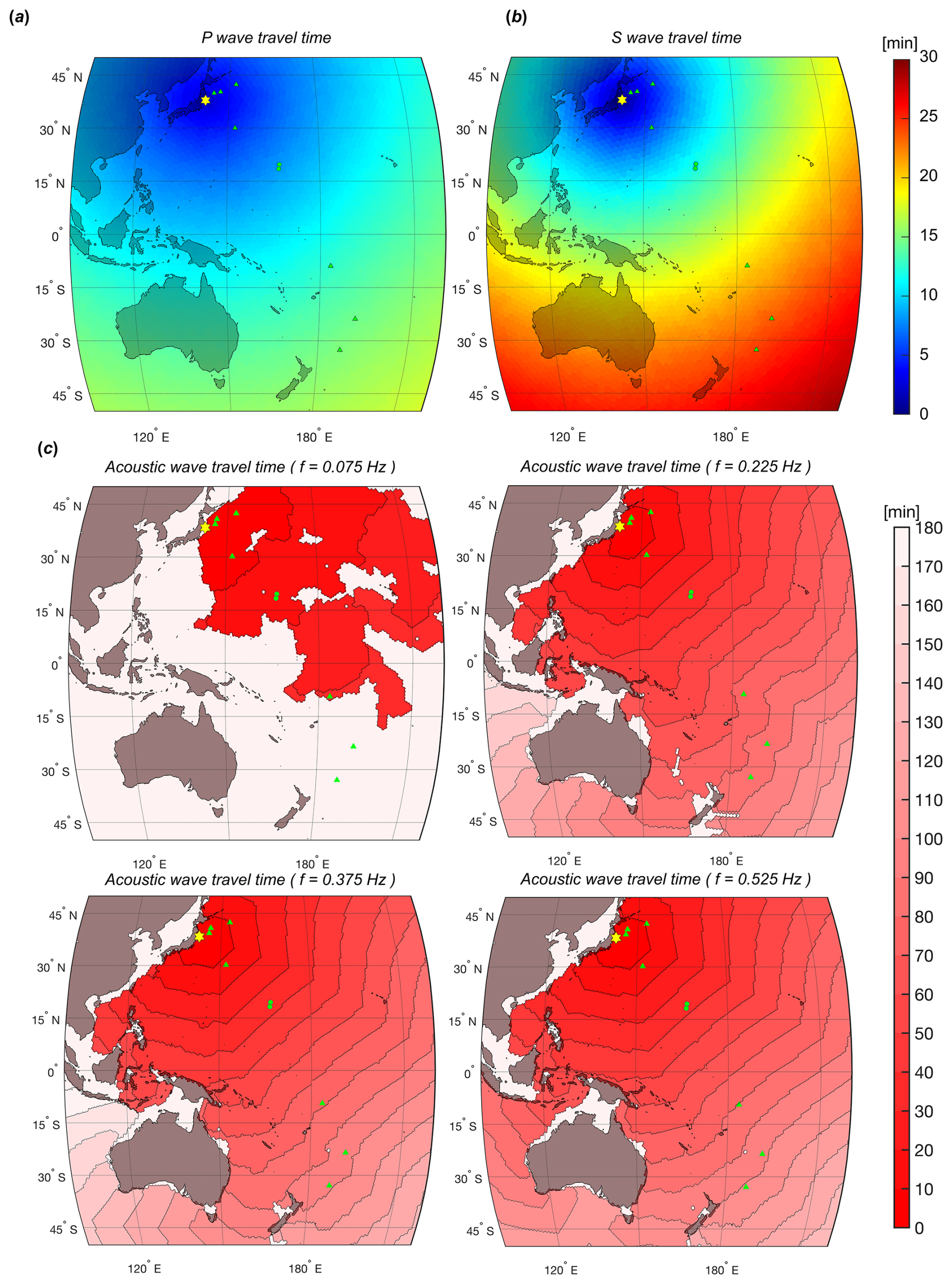
Figure 6 (a) P and (b) S wave travel times are computed using spatially varying compressional wave speed, c_p, and shear wave speed, c_s, derived from the PREM (Dziewonski and Anderson, 1981), with anisotropic variability in a spherical coordinate system (latitude, longitude), as described by Panning et al. (2010). (c) The travel times of the first four dominant acoustic modes (governed by fault depth). Bathymetry data from the General Bathymetric Chart of the Oceans (GEBCO) (Kapoor, 1981) are utilized to calculate arrival times for acoustic waves.

Figure 7 Surface tsunami travel times for the Tohoku 2011 event. Bathymetry data from the General Bathymetric Chart of the Oceans (GEBCO) (Kapoor, 1981) are used for the dispersion relation.

The detailed inverse problem model procedure can be found in Gomez and Kadri (2021). A comparison between input and calculated parameters by the inverse problem model can be found in Table II of Hendin and Stiassnie (2013) and Tables 3–4 of Gomez and Kadri (2021). However, as an example for calculating the distance from the effective fault, we consider the signal in Fig. 1 of the Sumatra earthquake test case. Note that the epicentre is located at a distance of about 2700 km from hydrophone H08S1. The specifics of the parameters employed in the inverse model are provided in the enlarged view depicted in Fig. 2. From Eqs. (8)–(9) we obtain x₀=2481 km, y₀=16 232 km, and thus a distance of 2965 km. Given the bearing of 64.5°±0.5°, the approximate location of the effective fault can then be found.

3 Software architecture and workflow

In order to facilitate the use of the technology in tsunami warning centres, as well as among the scientific community, we have been developing a user-friendly software, using the Python programming language. The software has been named GREAT (Global Real-time Early Assessment of Tsunami). It has the capability to automatically analyse incoming acoustic signals, keeping the option of manual use, with the aim to be employed both for real-time signal analysis and for educational purposes. A detailed description of the package, including the key considerations and the design philosophy that enables users to perform the analysis, the program structure, dependencies, and documentations, is given in Appendix E.

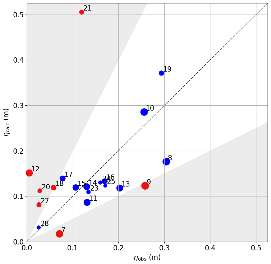
Figure 8 Tohoku 2011 study case, comparison of calculated amplitudes η_calc vs. observed amplitudes η_obs at various DART buoy locations. DART buoy location legend is given in Appendix F. Larger circles indicate shorter tsunami travel times to DART buoy locations, with the smallest circles representing around 10 h. Notably, most amplitude ratios fall within the range $\mathrm{0.5}<{\mathit{\eta }}_{\mathrm{calc}}/{\mathit{\eta }}_{\mathrm{obs}}<\mathrm{2}$. Blue circles mark DART buoy locations within this range, while red circles indicate locations outside it (see corresponding map in Fig. 9).

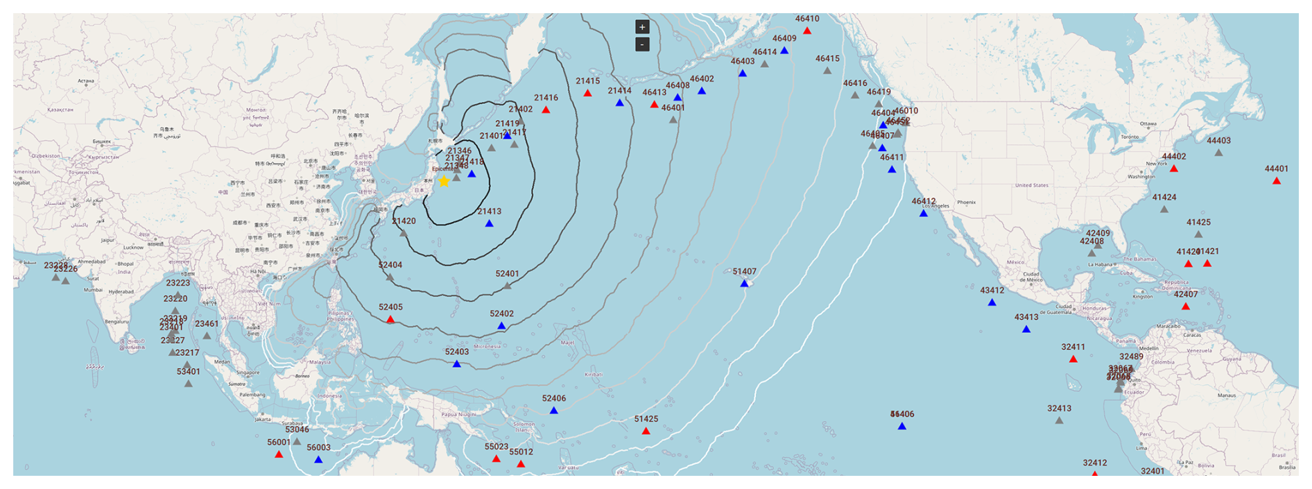
Figure 9 Tohoku 2011 DART buoy map. Blue triangles: location of DART buoys at which satisfactory agreement, up to a factor of 2, between calculations and observations (and vice versa), is noted. Red triangles: location of DART buoys at which larger deviations between calculations and observations are noted. Grey triangles: no available data. © OpenStreetMap contributors 2023. Distributed under the Open Data Commons Open Database License (ODbL) v1.0.

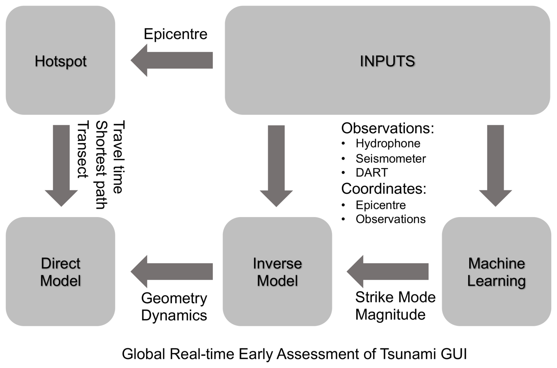
As shown in Fig. 3, the analysis begins by receiving information on the epicentre of the earthquake. Knowing its coordinates and the triangular mesh details, Dijkstra's shortest-path module calculates shortest paths from the epicentre to all nodes on the mesh and their corresponding transects. Using coordinates of all hotspots, the hotspot model calculates tsunami travel times, acoustic wave travel times, P and S waves, and the shortest paths from the epicentre to all hotspots and their corresponding transects. At this stage preliminary results are ready to be analysed, and initial warnings can, virtually, be issued.

The next required input is the signal (or multiple-signal) data and various analysis parameters for inverse and direct models. Operational software is designed to work with several signal input types. All of them are similar in terms of data structure as they contain arrays of pressure values, but they vary based on the file types. Those include Python NumPy array files (.npz), MATLAB data files (.mat), and text files with pressure values (.txt). Additionally, the system can take a json configuration file as an input, which will populate necessary analysis parameters alongside the signal data.

The signal data are used in a machine learning model to calculate additional earthquake parameters such as its magnitude and mode of strike. Alternatively, earthquake magnitude can be provided directly as an input if known. Then all the necessary parameters alongside the signal data are supplied to the inverse problem model, which returns probability density functions of the geometry and dynamics of the fault. Lastly, the inverse problem model results are used as input for the direct model that returns pressure and surface elevation data at all hotspot locations. After analysis is complete, the developed system generates an interactive map showing all the results and provides an option to save those into a file. There are two ways to export the results: one of them is a NumPy array file (.npz), and the other is a NetCDF4 file (Rew and Davis, 1990). Those can be used to load the results directly by the operational software to see the interactive map and full results at any convenient time or to analyse the results further using different software packages.

4 Results

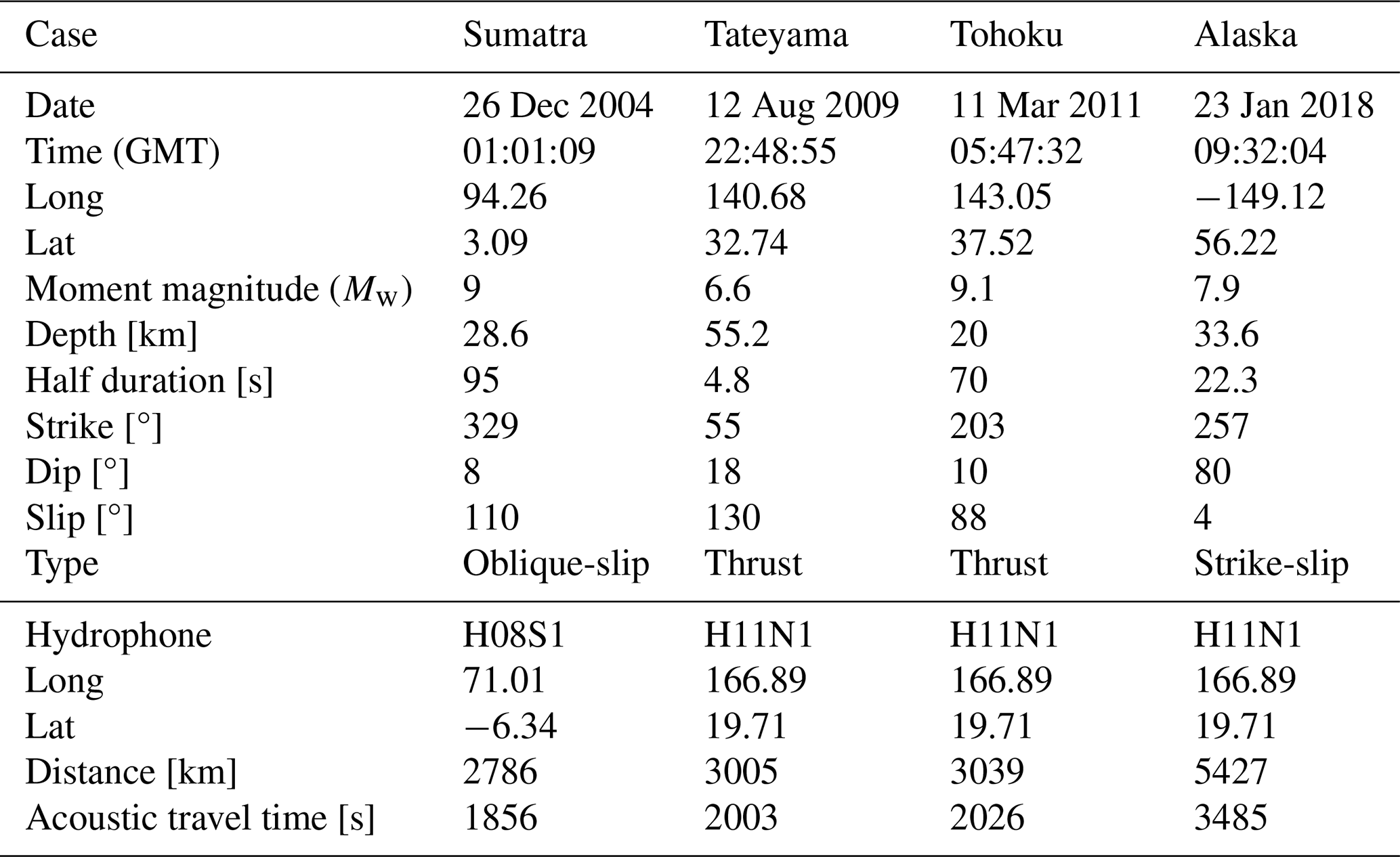
We present four test cases to highlight different qualities of the technology under development, with two cases resulting in mega-tsunamis and one that caused a major false alarm. The first test case is the 2004 M_w 9.1 Sumatra earthquake and tsunami. This test case highlights the promptness of the calculations and the timely assessment of the tsunami. It also shows some of the software GUI and main plotting features, but comparison with only five DART buoy data was made. The second test case is the Tohoku-oki 2011 tsunami. This test case emphasizes the results by the hotspot model. Quantitative analysis was done for all existing DART buoy data. The third test case concerns the 2018 M_w 7.9 Gulf of Alaska earthquake, which led to a false alarm. This test case emphasizes the capability of the presented technology to reducing the impact of false alarms. Quantitative analysis was done for existing DART buoy data. The last test case is the Tateyama 2009 event, which has a much smaller magnitude than the other test cases. This case is included to shed light on the effect of magnitude on the performance of the models. It is worth noting that all plots, apart from Figs. 8, 13, and 16), were made using the developed software (GREAT).

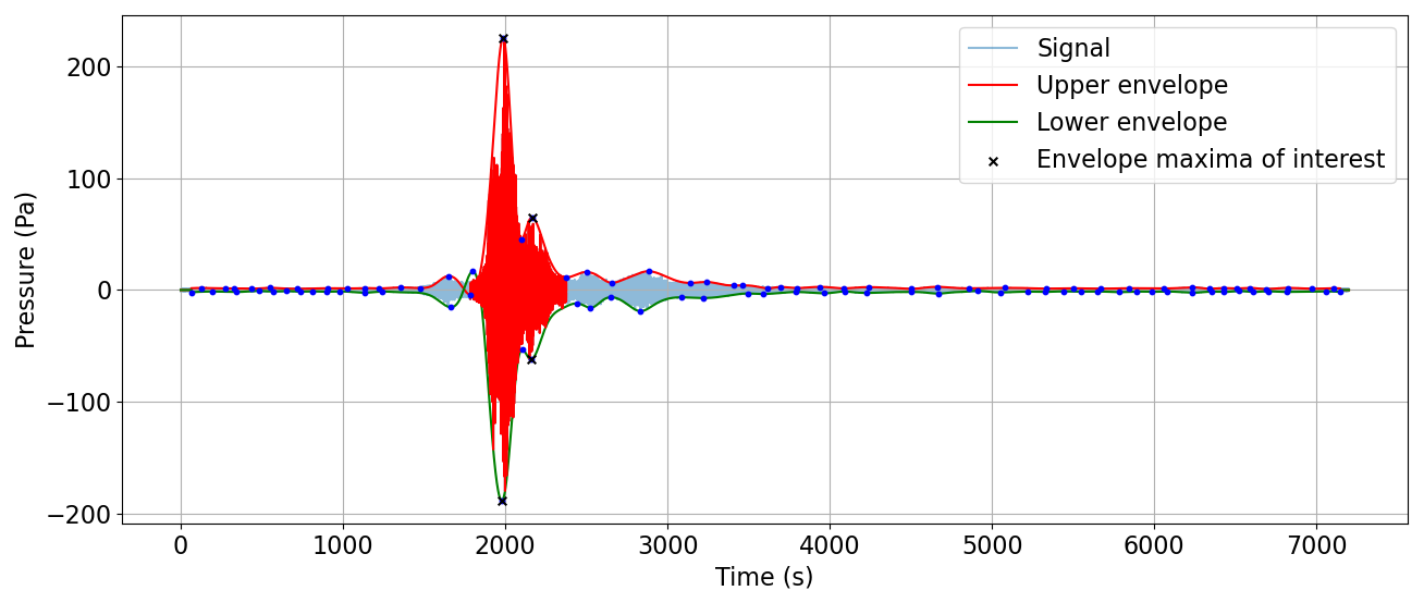
Figure 10 Test case 2018 M_w 7.9 Gulf of Alaska earthquake. Analysed pressure signal. The signal was recorded at CTBTO's hydroacoustic station at Wake Island, H11N. The analysis has been done automatically by the software for the region highlighted in red. The green and red curves are the lower and higher envelopes. The plot was created by the software GREAT.

Figure 11 Screenshots of the software (GREAT) for test case 2018 M_w 7.9 Gulf of Alaska earthquake. A snapshot from the software for showing tsunami evaluation contours at the coasts (red for high risk, yellow for middle risk/advisory, and green for no risk) at 50 m depth. Yellow star: earthquake epicentre. Green triangles: the location of current DART buoys. The hydrophone stations (H11S/H11N) are not shown. Hotspots: user-defined points of interest (green for no tsunami). © OpenStreetMap contributors 2023. Distributed under the Open Data Commons Open Database License (ODbL) v1.0.

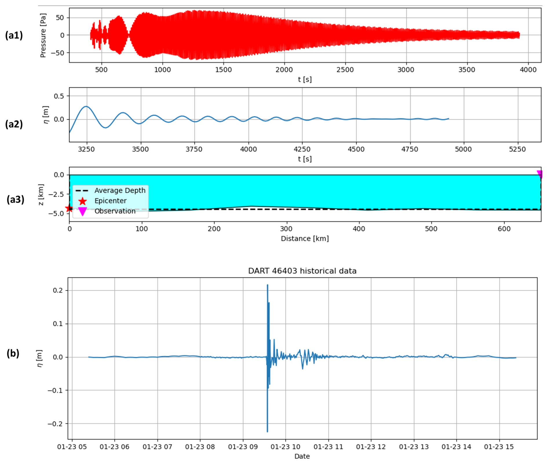
Figure 12 Test case 2018 M_w 7.9 Gulf of Alaska earthquake. The subplots in (a) were calculated by the software for the observation point at the location of DART 46403: (a1) pressure signal, (a2) water elevation, and (a3) sea bathymetry between the epicentre (star) and the observation point (triangle), with the average depth presented by a dashed line. Panel (b) is the observed water level at by DART 46403. These plots were created by the software GREAT.

4.1 Sumatra 2004

The 2004 Indian Ocean earthquake, which occurred on 26 December 2004, is one of the most powerful seismic events recorded in history. The undersea megathrust earthquake had a magnitude of 9.1–9.3 off the west coast of northern Sumatra, Indonesia (Lay et al., 2005). Triggering a series of devastating tsunamis, it affected more than a dozen countries, causing widespread destruction and killing 227 898 people in 14 countries (Goff and Dudley, 2021). The earthquake was caused by the subduction of the Indo-Australian Plate beneath the Eurasian Plate. The resulting displacement of the seafloor led to the release of a massive amount of energy, generating tsunamis that reached coastal areas across the Indian Ocean. The catastrophe highlighted the need for improved early warning systems and international collaboration in disaster preparedness and response.

Acoustic data related to the event were recorded on CTBTO hydroacoustic stations. The analysed pressure acoustic data (recorded on H08S1) are presented in Fig. 1. The analysis has been done automatically by the software for the region highlighted in red. The epicentre location is highlighted by a yellow star in Fig. 4. CTBTO hydroacoustic stations, H08S and H08N, are shown as blue circles, the tsunami arrival times are shown in black contours, and the location of DART buoys is presented by green triangles. The coloured contours in Fig. 4a near the shorelines present the relative tsunami amplitude (in metres), with red for tsunami threat (η>0.5), yellow for advisory ($\mathrm{0.2}<\mathit{\eta }<\mathrm{0.5}$), and green for no threat (η<0.2). These values that define the criteria for tsunami risk, referred to as the decision matrix in Fig. 4a, are typical values used by TWCs. The actual wave amplitudes are shown in Fig. 4b. Note that the hydroacoustic station is at a distance of about 3000 km, which is in a location that might be ideal for nuclear activity monitoring, though not for tsunami warning. If the hydroacoustic station were at a distance of 1000 km, that would have left enough alarm time, even for the closest shorelines that had as little as 15 min from the rupture time until the tsunami impact. The software successfully predicts most of the tsunami threat regions (red), even at very large distances such as Sri Lanka and Madagascar. The machine learning model predicted that this earthquake should generate a tsunami. The total analysis by all models took a few minutes on a standard multi-core PC station. There were no DART buoy data at the time of the event to allow a more quantitative analysis of the results. However a qualitative comparison with results shown by Lay et al. (2005) for five different locations is presented in Table 1. The calculations by the current model overpredict the observation by as little as 3 %, in the case of S. Maldives, to as high as 52 %, in the case of Banda Aceh.

4.2 Tohoku-oki 2011

The Tohoku-oki earthquake of 2011 was a momentous seismic event that struck off the northeastern coast of Japan on 11 March 2011. This megathrust earthquake, with a magnitude of 9.0–9.1, was caused by the Pacific Plate subducting beneath the North American Plate. The ensuing undersea earthquake triggered a massive tsunami that inundated the Japanese coastline and caused widespread devastation. The disaster resulted in the Fukushima Daiichi nuclear disaster, further intensifying the crisis.

The analysed acoustic data (recorded on H11N1) are presented in Fig. 5. As before, the analysis has been done automatically by the software for the region highlighted in red. The epicentre location is highlighted in Fig. 6 by a yellow star. The hydroacoustic stations H11S and H11N are shown as green circles. Note that the hydrophones are located at the SOFAR channel depth, about 700 m deep. The location of DART buoys is presented by green triangles.

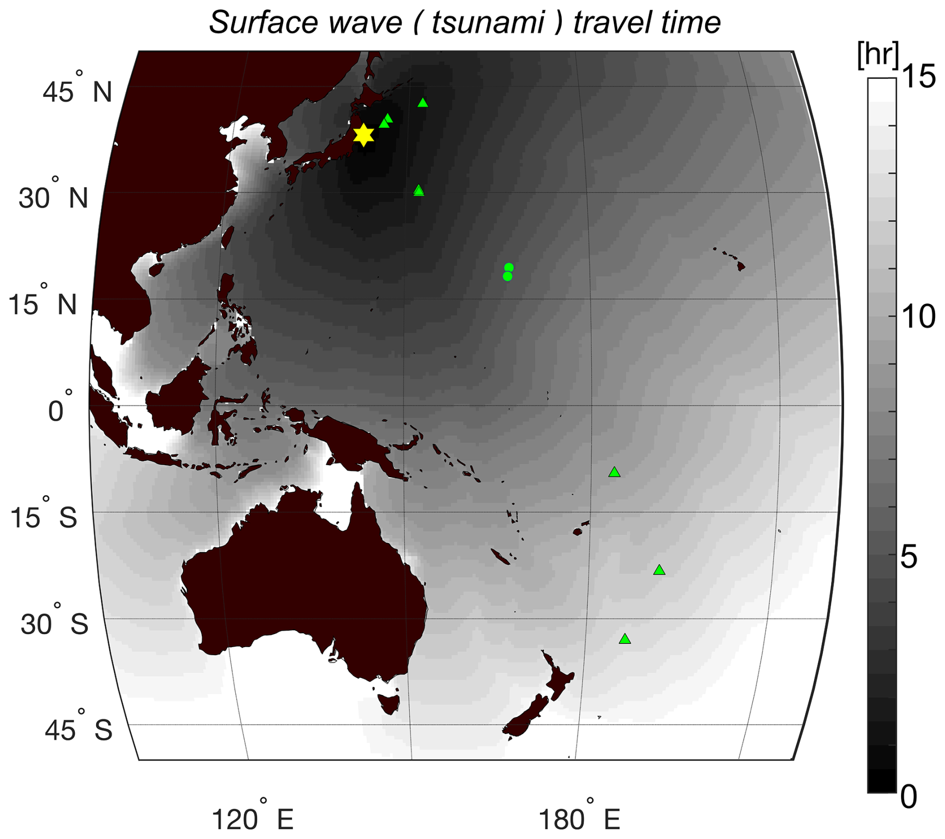
Figures 6 and 7 show the arrival time of three precursors and the surface gravity waves (tsunami) for Tohoku Oki 2011 event, calculated by the hotspot model. The arrival times of the P and S waves are presented in panels a and b, respectively, where spatially variable compressional c_p and shear wave c_s speeds are calculated from Lame's constants λ and μ of earth taken from the PREM (Dziewonski and Anderson, 1981), as shown in Eq. (1). Panel b shows the arrival time of the four first acoustic modes. In order to calculate the phase speed, the dispersion relation for compressible ocean is used (Abdolali and Kirby, 2017), as shown in Eq. (2). Figure 7 shows the arrival of tsunami waves where the dispersion relation for elastic half-space is used (Abdolali et al., 2019), as shown in Eq. (4).

To gain a more quantitative understanding of the performance of the models, we compare DART buoy observations, η_obs, with calculations, η_calc. Satisfactory agreement is in general observed at DART buoy stations closer to the epicentre and at stations with less land separating them from the epicentre – see Fig. 8 and the corresponding map in Fig. 9. The larger the circles, the lower the tsunami travel times to the DART buoy locations are, with the smallest circles representing approximately 10 h. For consistency, the DART buoys are numbered, and the real DART station names are provided in Appendix F. It is remarkable that the majority of the amplitude ratio falls within the region $\mathrm{0.5}<{\mathit{\eta }}_{\mathrm{calc}}/{\mathit{\eta }}_{\mathrm{obs}}<\mathrm{2}$. The blue circles represent DART buoy locations where the amplitude ratio falls within the specified range, while the red circles represent locations where the amplitude ratio is outside of this range.

4.3 Alaska 2018

The Alaska earthquake of 2018, which occurred on 23 January, was a significant seismic event with a magnitude of 7.9. Striking in the Gulf of Alaska, it raised concerns about potential tsunamis along the coast. The quake was attributed to the subduction of the Pacific Plate beneath the North American Plate. While the earthquake itself did not cause major damage or casualties, an error in the initial assessments led to a false alarm regarding a potential tsunami threat. The incident exposed flaws in the emergency alert system, demonstrating the importance of accurate and timely information dissemination during such events.

The analysed acoustic data (recorded on H11N1) are presented in Fig. 10. As before, the analysis has been done automatically by the software for the region highlighted in red. The epicentre location is highlighted in Fig. 11 by a yellow star. The tsunami assessment clearly shows that there is no tsunami threat in this case – green contours indicate no threat. The performance of the software can be assessed by comparing the calculated water elevation (tsunami amplitude) with DART buoys. For example, the peak amplitude recorded at DART 46403 is of the same order of the calculated amplitude (Fig. 12). It is also worth noting that the machine learning model predicted that this earthquake will not generate a tsunami. The prediction time took a fraction of a second, and the total analysis time by the inverse and direct models was less than 30 s on a standard multi-core PC station.

A quantitative analysis of the water elevation is shown in Fig. 13 corresponding to the map in Fig. 14. Again, consistent agreement is observed at DART buoy stations located closer to the epicentre, as well as at stations with less land separating them from the epicentre.

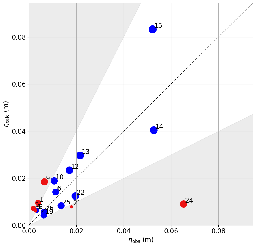
Figure 13 Alaska 2018 study case, comparison of calculated amplitudes η_calc vs. observed amplitudes η_obs at various DART buoy locations. DART buoy location legend is given in Appendix F. Consistent agreement is observed at DART buoy stations located closer to the epicentre, as well as at stations with less land separating them from the epicentre (see corresponding map in Fig. 14).

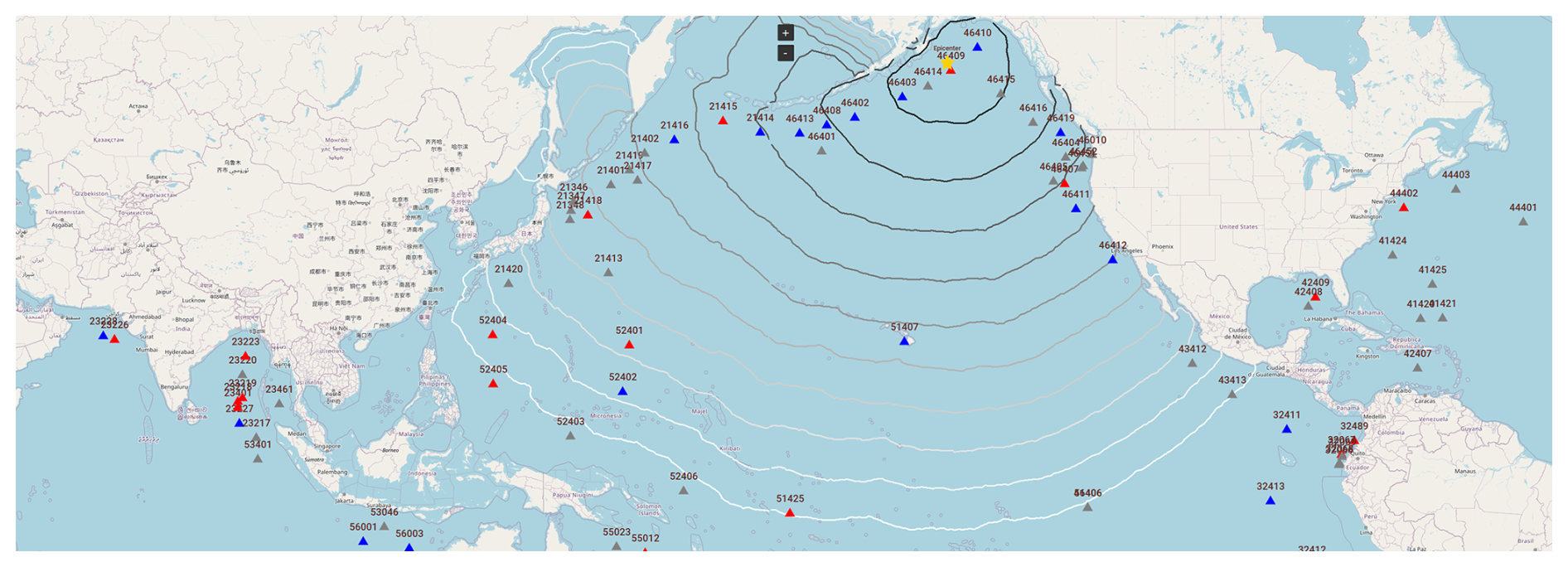
Figure 14 Alaska 2018 DART buoy map. Blue triangles: location of DART buoys at which satisfactory agreement, up to a factor of 2, between calculations and observations (and vice versa), is noted. Red triangles: location of DART buoys at which larger deviations between calculations and observations are noted. Grey triangles: no available data. © OpenStreetMap contributors 2023. Distributed under the Open Data Commons Open Database License (ODbL) v1.0.

4.4 Tateyama 2009

The Tateyama earthquake of 2009, with a magnitude of 6.6, struck approximately 244 km southeast of Tateyama, Japan. This seismic event occurred on 12 August 2009 and was associated with the subduction zone boundary between the Pacific Plate and the Philippine Sea Plate. The earthquake resulted in moderate shaking in the region and raised concerns about potential tsunami risks due to its offshore location. Again, the analysed acoustic data were recorded on H11N1, which is presented in Fig. 15. However, for this test case, we focus attention on the analysis of the water elevation, which is shown in Fig. 16, corresponding to the locations in the map in Fig. 17. Once again, consistent agreement is in general observed at DART buoy stations located closer to the epicentre, as well as at stations with less land separating them from the epicentre. It is also notable that in this relatively small earthquake, more deviation is noticed. This might be because the amplitudes are smaller and thus more sensitive to deviations.

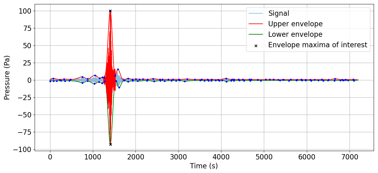
Figure 15 Test case 2009 M_w 6.6 Tateyama earthquake. Analysed pressure signal. The signal was recorded at CTBTO's hydroacoustic station at Wake Island, H11N. The analysis has been done automatically by the software for the region highlighted in red. The green and red curves are the lower and higher envelopes. The plot was created by the software GREAT.

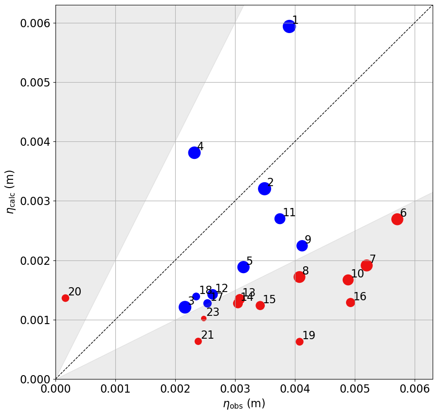
Figure 16 Tateyama 2009 study case, comparison of calculated amplitudes η_calc vs. observed amplitudes η_obs at various DART buoy locations. DART buoy location legend is given in Appendix F. Consistent agreement is generally observed at DART buoy stations nearer to the epicentre and those with minimal land separation from it (see corresponding map in Fig. 17). However, greater deviation is noted in this relatively small earthquake, likely due to smaller amplitudes being more sensitive to variations.

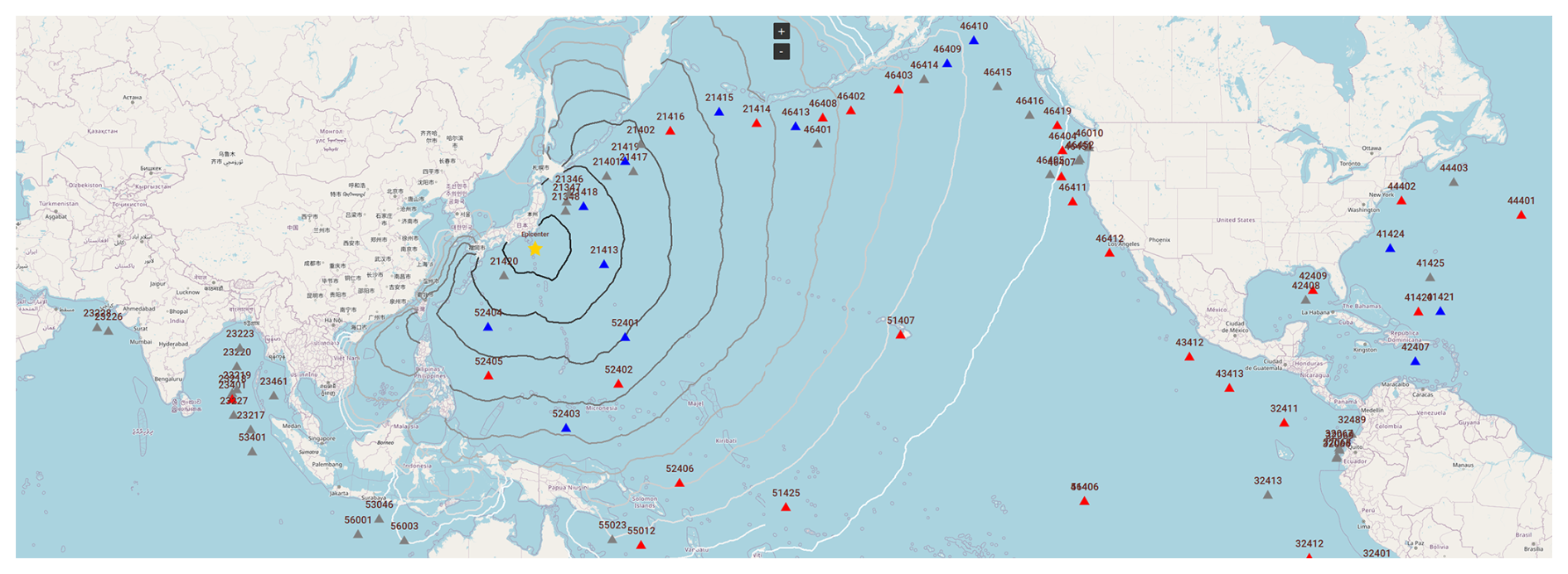
Figure 17 Tateyama 2009 DART buoy map. Blue triangles: location of DART buoys at which satisfactory agreement, up to a factor of 2, between calculations and observations (and vice versa), is noted. Red triangles: location of DART buoys at which larger deviations between calculations and observations are noted. Grey triangles: no available data. © OpenStreetMap contributors 2023. Distributed under the Open Data Commons Open Database License (ODbL) v1.0.

Table 2 Summary table for four case studies (Ekström et al., 2012).

Among the four case studies discussed in the paper, Sumatra was triggered by a large oblique-slip earthquake with a significant vertical component and prolonged duration, whereas Tohoku and Tateyama involved thrust fault movements. Tohoku was a high-magnitude, long-duration bottom-shaking event, while Tateyama was weaker and shorter in duration. In contrast, the Alaska case was characterized by a strike-slip fault, dominated by horizontal motion and moderately shorter duration compared to Sumatra and Tohoku. Despite its large magnitude, the horizontal motion in Alaska resulted in only a minor tsunami. The vertical ground motion played a critical role in tsunami generation for Sumatra, Tohoku, and Tateyama, whereas the horizontal motion in Alaska limited tsunami generation. Consequently, model performance depends heavily on earthquake magnitude and vertical motion, as defined by the dip angle, with better results observed for large, vertically dominant ground motions. Furthermore, the accuracy of model predictions improves when the gauges are closer to the hydrophones. The reason is that acoustic–gravity waves (AGWs) are less dissipated due to interactions with the seafloor geometry, allowing the inverse model to better capture and estimate the fault geometry. (see Table 2).

From an observational perspective, ground-truth data for the Sumatra case are limited to a few selected locations, as summarized in Table F1, while DART buoy observations were available for the Tateyama, Tohoku, and Alaska cases, as outlined in Table F2. The accuracy of the model at observation locations is further influenced by two key factors. The first is the ratio of the shortest distance to the direct distance (SD / DD) between the epicentre and the observation points; a ratio closer to 1 indicates wave propagation over relatively consistent depths, aligning well with the assumptions of the direct model. The second is the proximity of the observations to the source, as observations closer to the epicentre, reflected in shorter travel times, tend to show higher model accuracy.

5 Discussion

The methodology and software presented in this paper are aimed at providing a complementary tool in the domain of real-time early tsunami warning technology. By integrating state-of-the-art mathematical models and a machine learning model, our software has demonstrated, virtually, the capability of analysing sound signals to assess tsunamis globally, potentially in real time. The integration of data from diverse measurement sources has allowed for the dynamic mapping of high-risk areas, streamlining the identification of the shortest travel paths once the epicentre location is established. The machine learning model classifies earthquake magnitude and strike mode, while the incorporation of an inverse problem model has contributed to the calculation of probability density functions for fault geometry and dynamics. The calculated parameters are then employed by the direct model to provide tsunami amplitude assessment at high-risk locations, all accomplished within a computational time frame of seconds to a few minutes on standard multi-core PC stations.

However, it is important to acknowledge certain limitations in the presented technology. Notably, the dataset size of the machine learning model is relatively modest, encompassing only earthquakes that meet specific conditions. This limited dataset, while valuable for a proof of concept, does narrow the model's applicability to a specific subset of seismic events. Consequently, we view our research as a crucial initial step in demonstrating the potential of combining machine learning algorithms and semi-analytical solutions to infer properties of submarine tectonic events from acoustic radiation. The machine learning model can be improved in two ways. Firstly, employing a much larger database, the model can be trained to provide an angle of strike, instead of a binary result, i.e. vertical or horizontal. Secondly, the training can involve corresponding DART buoys as well as other sources, such as other tsunami measurements, including GPS buoys, tide gauges, or satellite altimeters. Incorporating these sources into the current version of the software, where they are primarily used for validation, can enhance confidence in model reliability across various geographical locations (offshore, nearshore, and at varying distances from the tsunami source). Such incorporation would exploit the database (since each event is associated with tens of DART buoys and other sources). Consequently, the model will be trained to assess the tsunami height at the different locations by analysing the acoustic signals directly, which is part of ongoing research. Once validated, the machine learning (ML) component in the next version of the model will be expanded to utilize these data as training datasets. This shift would alter their role from validation datasets to critical inputs, improving the model's predictive capabilities.

Integrating more datasets, including surface elevation from DART and GPS buoys, pressure from SMART cable and fibre optic cables, remote sensing (i.e. satellite altimetry), and acoustic waves, from sources other than CTBTO, can enhance the model and reduce uncertainty due to the sparseness of data. Increasing the number of datasets would enhance response time for faster warnings and provide multiple datasets per event, improving confidence in detection and analysis. It is important to note that certain components of the software, such as the inverse problem model, require adjustments based on the sampling rate. Therefore integrating publicly available data from sources like IRIS and Ocean Network Canada (ONC) requires system fine-tuning. During the expansion of the software to incorporate diverse and non-unified data types, a key challenge is ensuring that the software can distinguish data sources and account for differences in sampling rate, observational error, confidence level, and data format. Addressing these variations is crucial for accurate analysis and effective data integration.

Moreover, the presented quantitative analysis of the surface elevation (Figs. 8–9, 13–14, 16–17) indicates that the models perform relatively well, even at large distances. This is further supported by Fig. 18, which shows good agreement between amplitude ratios and tsunami travel times for the Tateyama 2009, Tohoku 2011, and Alaska 2018 events across various DART buoy locations, with a travel time limit of 24 h. To mitigate minor arbitrary fluctuations in wave amplitude measurements, a constant offset of 0.05 m is added to all values. A challenge with DART buoys is their hybrid sampling rate, which is too low [Δt=15 min] under normal conditions and only increases [Δt=1 min, 15 s] if triggered above a certain threshold. Typically, at these locations, the DART buoys are not triggered, resulting in a low sampling rate and data dominated by irrelevant noise. However, there is a need to analyse many more events, as well as studying results at each DART buoy location individually, before a solid conclusion is established, and the software becomes fully operational. It must be noted that the inverse problem model analysis conducted here was done automatically, whereas a more careful selection of the analysed envelopes could largely improve the results.

To enhance the operational capabilities of the software and its real-time analysis, it has been deployed since June 2024 at the Tsunami Warning Centre of the Instituto Português do Mar e da Atmosfera (IPMA), where it has access to real-time hydrophone data provided by CTBTO. This deployment aims to assess the system's performance under operational conditions, addressing key challenges such as hardware limitations, data transmission delays, and potential sensor failures. A detailed evaluation of these factors is ongoing, with results to be published upon the study's completion.

Note that a major limitation of the current real-time assessment is the sparse distribution of hydrophone stations. CTBTO operates six hydrophone stations globally, of which access is currently available for only four. The geographic distribution of these hydrophones restricts the technology's applicability to specific regions. The system is most effective within a 1000 km radius of each station, enabling an end-to-end assessment within an average of less than 6 min. Using these figures as an indicator for optimized global hydrophone station density, approximately 30 hydrophone stations would be required.

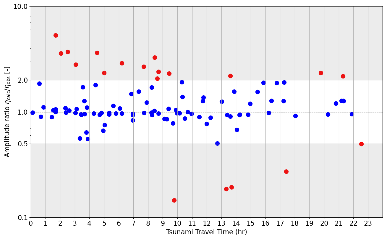
Figure 18 Amplitude ratio against tsunami travel time for Tateyama 2009, Tohoku 2011, and Alaska 2018 study cases at various DART buoy locations with tsunami travel time up to 24 h.

In conclusion, our work represents a complementary approach towards more effective early tsunami warning systems. While we acknowledge certain limitations, our methodology and software provide a robust foundation upon which future research and enhancements can be built. We hope this work encourages further research and development and provides a platform for integrating other efforts, both conservative and innovative, that would contribute to the overarching goal of ensuring the safety and resilience of coastal communities worldwide.

Appendix A: Coefficients C₁, C₂, and C₃

$$\begin{array}{}\text{(A1)}& {\displaystyle }{C}_{\mathrm{1}}={\mathit{\omega }}^{\mathrm{2}}/rg-{\mathit{\gamma }}_l/r,\text{(A2)}& {\displaystyle }{C}_{\mathrm{2}}=[q+{\mathit{\gamma }}_p]{\mathit{\rho }}_l\left({\displaystyle \frac{k^{\mathrm{2}}-s^{\mathrm{2}}-\mathrm{2}s{\mathit{\gamma }}_{\mathrm{s}}-{\mathit{\gamma }}_{\mathrm{s}}^{\mathrm{2}}}{k^{\mathrm{2}}+s^{\mathrm{2}}+\mathrm{2}s{\mathit{\gamma }}_{\mathrm{s}}+{\mathit{\gamma }}_{\mathrm{s}}^{\mathrm{2}}}}\right),\text{(A3)}& {\displaystyle }\begin{array}{rl}{C}_{\mathrm{3}}& =\left({\displaystyle \frac{\mathrm{4}\mathit{\mu }{k}^{\mathrm{2}}[s+{\mathit{\gamma }}_{\mathrm{s}}][q+{\mathit{\gamma }}_p]}{k^{\mathrm{2}}+s^{\mathrm{2}}+\mathrm{2}s{\mathit{\gamma }}_{\mathrm{s}}+{\mathit{\gamma }}_{\mathrm{s}}^{\mathrm{2}}}}+({\mathit{\rho }}_{\mathrm{s}}{\mathit{\omega }}^{\mathrm{2}}-\mathrm{2}\mathit{\mu }{k}^{\mathrm{2}})\right.\\ & \left.-\mathrm{2}{\mathit{\gamma }}_p(q+{\mathit{\gamma }}_p)(\mathit{\lambda }+\mathrm{2}\mathit{\mu })\right),\end{array}\end{array}$$

where ρ_l is the water density.

Appendix B: Dijkstra's algorithm

The Dijkstra algorithm works on graphs that have non-negative weights on their edges. It uses a greedy approach to iteratively explore nodes and update the shortest-path distances from the starting node to all other nodes. The algorithm maintains a set of “visited” nodes and a priority queue, initially containing only the starting node with a distance of zero.

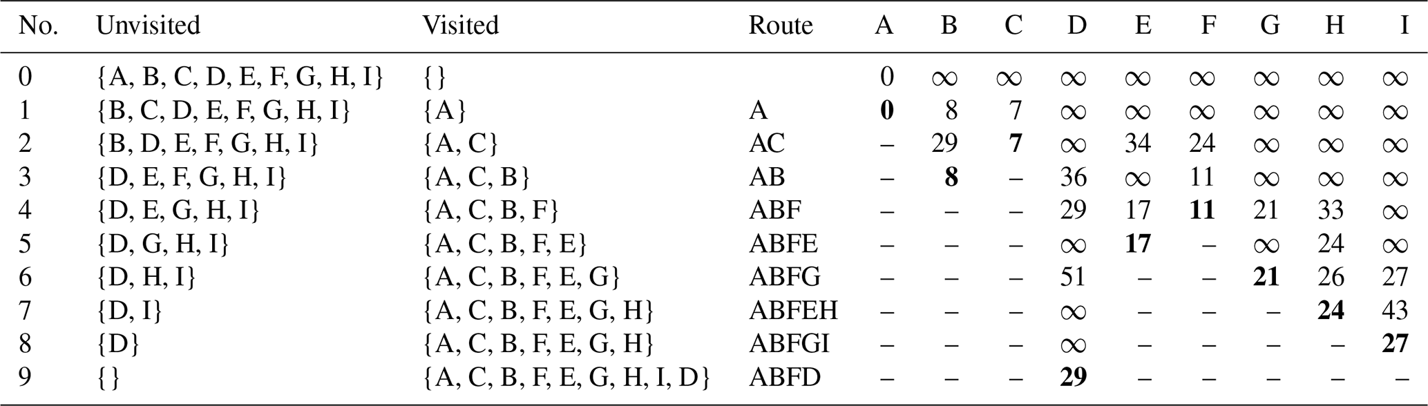
Table B1 Dijkstra's algorithm for the source at point A and shortest-path (blue) calculation to the destination points on the graph, shown in Fig. B1. The bold text is the shortest travel time from the source point (A).

Here are the main steps of Dijkstra's algorithm, adapted for P, S, acoustics, and tsunami waves:

1. Initialize the distance from the starting node to all other nodes as infinity (or a very large value) except the starting node itself, which is set to 0. Also, set the starting node as the current node.

2. While there are unvisited nodes, mark the current node as visited.

3. Update the distance of all neighbouring nodes that are not yet visited. The new distance is calculated as the minimum of the current distance to the neighbour and the sum of the distance from the current node to the neighbour (edge weight).

4. Choose the unvisited node with the smallest distance as the next current node, and repeat step 3.

Once all nodes have been visited or there are no more reachable nodes, the algorithm terminates, and the distances calculated are the shortest-path distances from the starting node to all other nodes in the graph. Upon completion, the algorithm produces a set of distances that represent the shortest path from the starting node to all other nodes in the graph. By following the sequence of nodes that produce these distances, the actual shortest paths are reconstructed. A schematic view of a triangular mesh, connectivity between nodes, and edge weight is shown in Fig. B1, and the Dijkstra algorithm, applied to find the shortest path between the source node (A) and the rest of nodes, is given in Table B1. Note that the calculation of tsunami and acoustic wave travel times occurs on an unstructured mesh spanning the Earth's surface, facilitating the propagation of these waves across the planet's exterior. Meanwhile, a three-dimensional mesh is employed for the modelling of P and S waves, enabling the propagation of P waves through the Earth's mantle, outer, and inner core and S waves through the mantle.

Figure B1 Schematic view of nodes' connectivity (grey lines) and weight (travel time).

Appendix C: Envelope equation

The envelope in Eq. (6) is given by Mei and Kadri (2018)

$$\begin{array}{}\text{(C1)}& \begin{array}{rl}& A(k,X,Y)=\\ & {\displaystyle \frac{\mathrm{1}-\mathit{ı}}{\mathrm{2}}}\left[C\left(z\right)\left(\sqrt{{\displaystyle \frac{\mathrm{2}}{\mathit{\pi }\mathcal{X}}}{\mathcal{Y}}_{+}}\right)+C\left(z\right)\left(\sqrt{{\displaystyle \frac{\mathrm{2}}{\mathit{\pi }\mathcal{X}}}{\mathcal{Y}}_{-}}\right)\right]\\ & +{\displaystyle \frac{\mathrm{1}+\mathit{ı}}{\mathrm{2}}}\left[S\left(z\right)\left(\sqrt{{\displaystyle \frac{\mathrm{2}}{\mathit{\pi }\mathcal{X}}}{\mathcal{Y}}_{+}}\right)+S\left(z\right)\left(\sqrt{{\displaystyle \frac{\mathrm{2}}{\mathit{\pi }\mathcal{X}}}{\mathcal{Y}}_{-}}\right)\right],\end{array}\end{array}$$

where C(z) and S(z) are Fresnel integrals (Lozier, 2003),

$$\begin{array}{}\text{(C2)}& \mathcal{X}={\displaystyle \frac{X}{\mathrm{2}{k}_n}},\mathrm{2}{\mathcal{Y}}_{+}=l+Y,\mathrm{2}{\mathcal{Y}}_{-}=l-Y.\end{array}$$

Appendix D: Stationary phase approximation

To obtain the stationary phase approximation we consider the phase term Γ₀(ω) for the general case (following Williams et al., 2021):

$$\begin{array}{}\text{(D1)}& \begin{array}{rl}{\mathrm{\Gamma }}_{\mathrm{0}}\left(\mathit{\omega }\right)& =k_{\mathrm{0}}\left(\mathit{\omega }\right){\displaystyle \frac{x}{t}}-\mathit{\omega },{\mathrm{\Gamma }}_{\mathrm{0}}^{\prime }\left(\mathit{\omega }\right)=k_{\mathrm{0}}^{\prime }\left(\mathit{\omega }\right){\displaystyle \frac{x}{t}}-\mathrm{1}=\mathrm{0},\\ & {\mathrm{\Gamma }}_{\mathrm{0}}^{\prime \prime }\left(\mathit{\omega }\right)=k_{\mathrm{0}}^{\prime \prime }\left(\mathit{\omega }\right){\displaystyle \frac{x}{t}},\end{array}\end{array}$$

where single and doubles primes denote first and second derivatives with respect to ω:

$$\begin{array}{}\text{(D2)}& k_{\mathrm{0}}^{\prime }={\displaystyle \frac{\mathrm{1}}{k_{\mathrm{0}}}}\left({\displaystyle \frac{\mathit{\omega }}{c^{\mathrm{2}}}}+r_{\mathrm{0}}{r}_{\mathrm{0}}^{\prime }\right).\end{array}$$

The stationary phase approximation requires a second derivative of k₀,

$$\begin{array}{}\text{(D3)}& k_{\mathrm{0}}^{\prime \prime }\left(\mathit{\omega }\right)={\displaystyle \frac{\mathrm{1}}{k_{\mathrm{0}}}}\left({\displaystyle \frac{\mathrm{1}}{c^{\mathrm{2}}}}+{\left(r_{\mathrm{0}}^{\prime }\right)}^{\mathrm{2}}+r_{\mathrm{0}}{r}_{\mathrm{0}}^{\prime \prime }\right)-{\displaystyle \frac{\mathrm{1}}{k_{\mathrm{0}}^{\mathrm{2}}}}\left({\displaystyle \frac{\mathit{\omega }}{c^{\mathrm{2}}}}+r_{\mathrm{0}}{r}_{\mathrm{0}}^{\prime }\right)k_{\mathrm{0}}^{\prime }.\end{array}$$

Appendix E: Software development

E1 Program structure

The operational software was written using the Python programming language, which was chosen as it has numerous libraries and frameworks that can handle complex mathematical operations quickly and efficiently. That makes it a top choice programming language for the development of any kind of scientific application (Raschka et al., 2020). It is highly memory-efficient and easy to write and debug. Additionally, it is fully cross-platform, which is one of the key requirements of the operational software. The software can be compiled on Unix, Mac, and Windows operational systems and is scalable on high-performance computing (HPC) platforms that are conventionally used in forecast centres.

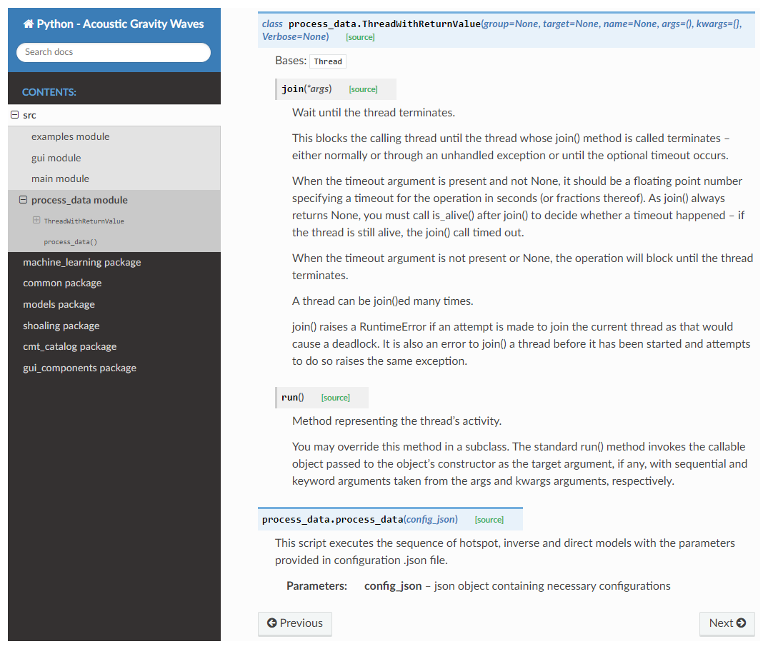
Figure E1 An excerpt from the documentation of the Global Real-time Early Assessment of Tsunami software.

The developed system has a modular structure, with each model written as an independent component. These modules include the machine learning model, inverse problem model, direct model, and hotspot model (Dijkstra's shortest-path algorithm). Many other functions that the main modules are dependent on are also implemented as modules in order to simplify the code and reuse as much existing knowledge as possible. These functions include basic functionality to read data, calculate distances between points on the map, extract contours from meshes, etc. The modular structure allows convenient and efficient adjustment to various parts of the system without breaking core software functionality.

To further increase the efficiency of the developed system and produce high-quality results in less time, calculations are done in parallel. Parallelization is applied to both inverse and direct models. Inverse problem model calculations are concurrently performed for all signals with the probability density functions of the geometry and dynamics of the fault combined after all the signals are fully analysed. The direct model is concurrently applied to all the hotspots in batches depending on the total number of hotspots supplied into the system. To achieve the required high efficiency, the concurrent.futures Python module is used for parallelization. On top of being effective, it provides a convenient way of asynchronous execution of tasks with both threads and processes (Sodian et al., 2022). Additionally, it allows Python to automatically scale calculations depending on the available computational power, number of CPUs, etc. That makes operational software highly efficient on all kinds of systems and helps it utilize its full potential.

E2 Dependencies

As Python offers an extensive collection of libraries that simplify complex computations and data analysis, the developed system depends on some of the external packages. All the packages are open-source, free, and maintained by their respective developers and the community. These include popular and highly efficient packages such as NumPy and SciPy. NumPy is a numerical mathematics extension of Python, which adds support for multi-dimensional arrays, along with a number of high-level mathematical operations on these arrays. SciPy is an extension of NumPy and provides more specific mathematical algorithms and convenience functions that are used in the main modules of the developed software. Machine learning is performed using the scikit-learn Python library, which is designed on top of NumPy and SciPy packages and features various classification, regression, and clustering algorithms.

A Matplotlib package is used for visualization purposes. This is a general and comprehensive plotting library for Python and NumPy, which can be used for creating both static and interactive figures. Python supports a number of graphical user interface (GUI) development frameworks. Among these, Tkinter was chosen as it is a free GUI framework best suited for developing desktop stand-alone applications. It is minimalistic and easy to use, and it is built on top of a Python standard GUI framework with a vast collection of widgets covering all the needs of the operational software development. To keep the GUI as consistent as possible while keeping the modern look, the developed system depends on the CustomTkinter library (https://customtkinter.tomschimansky.com/documentation/, last access: 17 April 2024).

E3 Documentation

Writing adequate documentation is an important aspect of continuous software development that helps future users and developers of the software. A comprehensive documentation using the Python Sphinx documentation generator was developed alongside the operational software. It automatically transforms descriptions of each function functionality and inputs and outputs into an interactive documentation HTML website with many convenient additions, i.e. contents index and search. This website can be easily rebuilt when any adjustments are made to the code. An excerpt from the documentation is shown in Fig. E1. It provides the opportunity to transition into an open-community paradigm, where parallel development is under consideration, following best practice coding standards. The main advantages of using an automated documentation generator are that the documentation is non-intrusive and is never out of sync. This way, coding and documenting are a part of the same task and are performed simultaneously (Theunissen et al., 2022).

Appendix F: DART buoy station legend

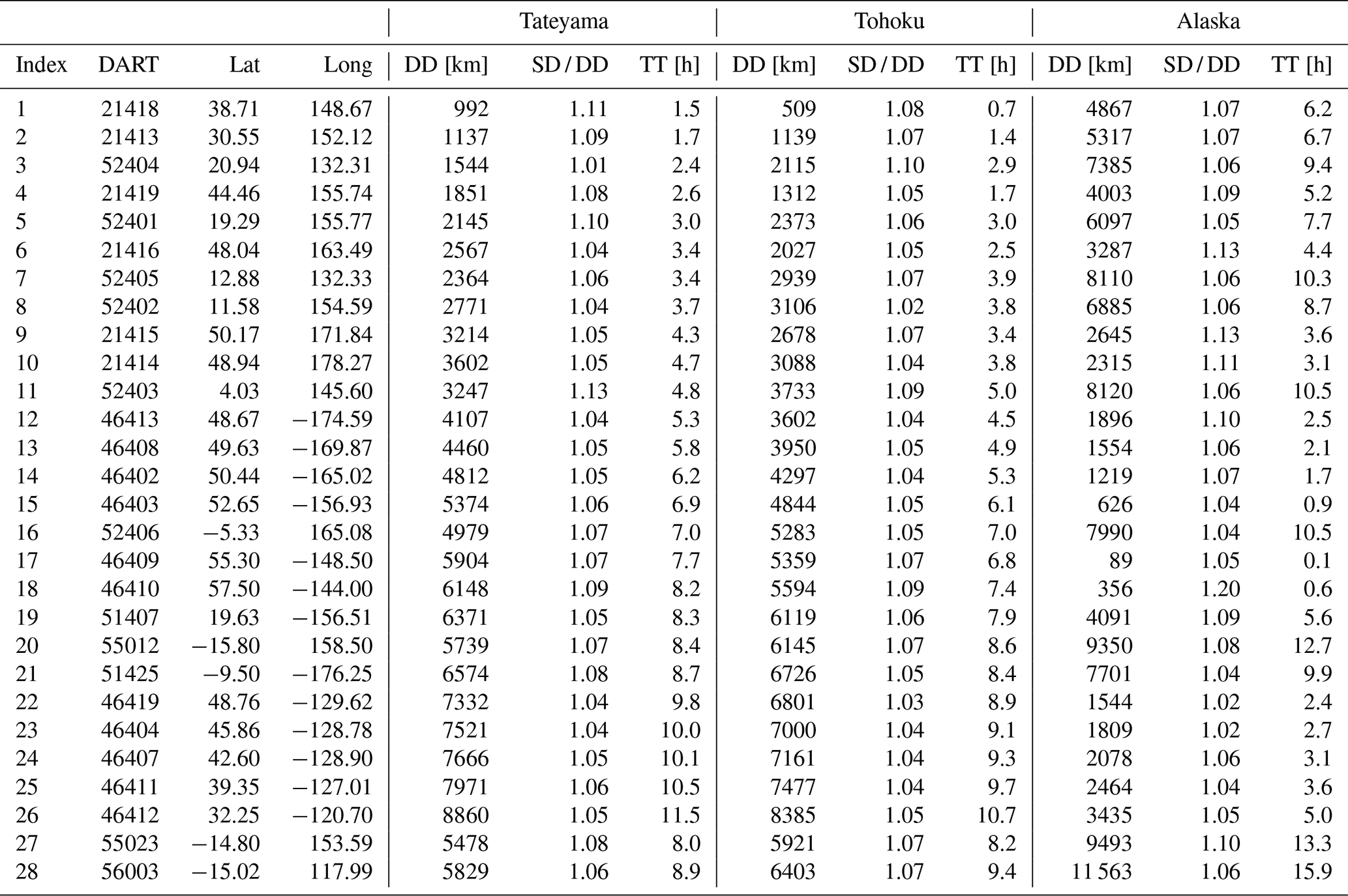
DART buoy station locations are coded according to Table F2.

Table F1 Direct distance (DD), ratio of shortest distance to direct distance (SD / DD), and travel time (TT) for Sumatra 2004.

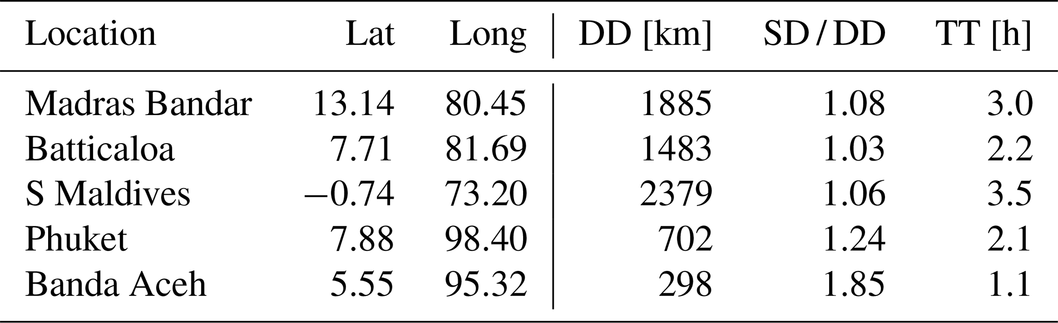
Table F2 DART buoy stations legend: direct distance (DD), ratio of shortest distance to direct distance (SD / DD), and travel time (TT) for Tateyama 2009, Tohoku 2011, and Alaska 2018 events.