A reach-integrated hydraulic modelling approach for large-scale and real-time inundation mapping

Flooding is one of the world's most common and costly natural hazards, inflicting billions in damages each year. However, current hydraulic models to support flood mapping are not well suited for large-scale applications or frequent updates, either due to limited accuracy of simple methods or lack of scalability (i.e. large computational requirements) for more sophisticated hydrodynamic models. This results in flood maps being decades out of date or simply nonexistent in some areas. Recent advances in generating flood maps have been made seemingly in parallel between geospatial methods and hydrodynamic models, such as the Height Above Nearest Drainage (HAND) method, hybrid 1D–2D hydrodynamic models, and more efficient computing of 2D models. This study presents the Geospatially Augmented Standard Step (GASS) method, which combines a novel improvement to the HAND method, Dynamic Height Above Nearest Drainage (DHAND), with a 1D hydraulic model for rapid flood inundation mapping at large scales while maintaining the accuracy of hydrodynamic models. This method is implemented into a new modelling software package called Blackbird and is tested via verification of the code and a benchmark case study comparing multiple approaches in the ability to approximate 2D model results. The Blackbird model vastly outperforms the simpler HAND–Manning method and also outperforms a traditional HEC-RAS 1D model when evaluated for accuracy of approximating a 2D model benchmark. This new method is shown to reduce the incidence of falsely predicting flooded areas through improved resolution of landscape connections over HAND-based or 1D hydraulic models. Blackbird also streamlines the model development effort relative to existing 1D or 2D models while maintaining a computational speed that was 10 000 times faster (a few seconds compared to a few hours) than a comparable 2D model in one case study. The method also allows for future integration of hydraulic structures, ice jams, and other features that are unavailable in HAND-based models. Overall, the GASS method provides a viable option for large-scale and real-time fluvial flood mapping applications.

1 Introduction

Flooding is one of the most common and costly natural hazards, with expected trends showing an increase in both exposure and vulnerability to flooding globally (e.g. Bhupsingh et al., 2022; Aristizabal et al., 2023; Steinhausen et al., 2022). As an example, the total residential flood risk in Canada is estimated to be CAD 2.9×10¹² yr⁻¹ by Public Safety Canada (Bhupsingh et al., 2022), while the availability of flood maps in high-risk Canadian communities is ranked as poor (Henstra et al., 2019). There is a need to mitigate flood risk for both the protection of human lives but also against financial losses. While there are different types of flooding (largely categorized as fluvial, pluvial, coastal, and minor system flooding including sewer backups), here we focus on addressing fluvial or riverine flooding (i.e. flooding that results from the overtopping of river banks as the river's capacity is exceeded).

Tools for mitigating flood risk and estimating flood extent come in different forms. For example, satellite imagery can be used to derive near-real-time or rapid flood maps (e.g. Tripathy and Malladi, 2022; Cian et al., 2018). These approaches are based on comparing satellite imagery during flood events to dry events and delineating flooded areas based on the differences in imagery. The availability of social media and other online information has also been exploited through machine-learning approaches and data mining to help determine active flood locations (e.g. Lin et al., 2023; Li et al., 2018; Fohringer et al., 2015). While these techniques may be useful in obtaining near-real-time conditions, they are not useful in prediction or simulation of future or possible flood impacts, as they rely on the collection of data in the period during and shortly after flooding occurs. In order to obtain simulations or forecasts of flooding, particularly under conditions not observed in the historical record, numerical models that can estimate future or hypothetical conditions are required.

Existing hydrodynamic models based on mass, energy, and momentum conservation, such as HEC-RAS (Hydrologic Engineering Center, 2023), have been used extensively to develop flood maps. These typically involve a numerical solution to the shallow-water equations, either in one dimension (1D) or two dimensions (2D). The results of 1D models can be imputed in space to create flood maps, though imputation is frequently done with an external program such as HEC-GeoRAS or external GIS software, (e.g. Yang et al., 2006; Md Ali et al., 2015; Hashim et al., 2021), and issues exist in the ease of generation and the interpretation of these results from 1D models with cross-sections. These include the prediction of wetted areas in locations with no hydraulic connection to the channel, caused by linear interpolation of water surface elevations (Bates, 2022). The accuracy of 2D models is generally considered much higher, with a number of studies confirming the benefit of 2D models over 1D in most circumstances (Ghimire et al., 2022; Jafarzadegan et al., 2023). In addition, 2D models do not require interpolation in the same way as 1D models since results are already spatially distributed. However, 2D models have a number of drawbacks, including high effort to configure and a high computational expense, and are therefore difficult to implement at large scales. Recent research efforts have focused on improving the efficiency of 2D models, including use of simplified forms of the underlying shallow-water equations, hybrid 1D–2D approaches, code optimization, and leveraging the use of high-performance computing (Jafarzadegan et al., 2023). Other approaches have also attempted to use machine-learning tools either to emulate 2D model results (e.g. Kabir et al., 2020; Zhou et al., 2022) or to simulate inundation directly (e.g. Shaeri Karimi et al., 2019; Frame et al., 2024). Global flood maps have also been produced at an approximate resolution of 90 m using the 2D LISFLOOD-FP model (Sampson et al., 2015). In all of these cases, the high degree of effort and computational cost of running the hydrodynamic models remains a barrier in practice, particularly for large-scale, high-resolution, and/or real-time prediction. Recent near-real-time forecasting applications seem to have overcome this barrier through massive parallelization and leveraging of graphical processing units (GPUs) (e.g. Apel et al., 2022; Najafi et al., 2024).

The computational demands of hydrodynamic models have at least partially driven the development of simplified methods for flood inundation and mapping (Hamidi et al., 2023). Many simplified methods focus on use of high-resolution topographic data to estimate flood depths. The most basic version of this could be considered the planar method, where any raster pixel with an elevation less than a specified flood elevation is considered flooded (Teng et al., 2015; McGrath et al., 2018). Other examples of recent simplified methods include the rapid flood spreading method (Lhomme et al., 2009), AutoRoute (Follum, 2013), and the Height Above Nearest Drainage (HAND) model (Rennó et al., 2008; Nobre et al., 2011). The popular HAND approach and its derivatives have been used in many studies (e.g. McGrath et al., 2018; Tavares da Costa et al., 2019; Scriven et al., 2021; Chaudhuri et al., 2021; Aristizabal et al., 2023) as a low-complexity, low-computational-cost approach to estimating flood depths and inundation extents, which is also scalable to large domains. The HAND approach re-expresses an elevation raster in terms of relative elevation to the nearest drainage point, which can then be used to rapidly generate inundation maps with depths for each drainage feature provided. Approaches in the literature for generating these depth estimates typically deploy Manning's equation to develop synthetic rating curves that estimate depth from flow (e.g. Afshari et al., 2018; Scriven et al., 2021; Chaudhuri et al., 2021; Diehl et al., 2021) and rely on the calculation of hydraulic properties over a reach to estimate wetted perimeter and area in Manning's equation (Zheng et al., 2018a, b). This type of approach, referred to here as the HAND–Manning method, has been shown to work reasonably well at emulating results of more sophisticated models in relatively simple cases, but since each reach is computed independently, the approach struggles with the very common case where backwater effects influence results (Aristizabal et al., 2023). Hydraulic structures can also not be represented with this approach. In addition, these methods do not respect mass, energy or momentum conservation. Other studies have circumvented these particular issues by calculating depths at cross-sections using HEC-RAS and then mapping these depths using HAND rather than interpolating results between cross-sections (Li et al., 2023). However, this approach assumes that the information at cross-sections is representative of conditions along the entire reach without considering the reach data in hydraulic calculations, which may not be appropriate in all cases.

In this study, we introduce a novel approach that combines the inundation mapping capabilities of the HAND approach with a 1D steady-state hydraulic model capable of handling backwater effects. We also provide a variant of the HAND approach, the Dynamic HAND (DHAND), which improves upon the ability of HAND to capture landscape connections within the DEM. The HAND or DHAND approaches are used in estimating hydraulic properties for 1D calculations, such as conveyance and cross-sectional flow area, and in mapping the depth results, thus removing the need for cross-sections that are typically deployed in 1D hydrodynamic models. This overcomes the limitations of HAND-only approaches with no backwater effects or energy loss calculations, and it also integrates the complete set of 3D information into the hydraulic model rather than relying on cross-sections to extract local data. The HAND-based method is used both in determining hydraulic properties for the hydraulic model (rather than from a cross-section) and in mapping the depth results in post-processing. These methods are combined within the Geospatially Augmented Standard Step (GASS) method and implemented within the Blackbird software package.

The main objectives of this study are

1. to present of a methodology that utilizes the reach-integrated approach and the HAND model to represent hydraulic properties and combine it within a 1D hydraulic model,

2. to introduce a modified version of HAND that captures the landscape connectivity as a function of stage and improves upon the ability of HAND to capture landscape connections in complex terrains, and

3. to demonstrate of the ability of the Blackbird software (which implements the GASS method) to estimate channel depths by first verifying the code against standard cross-section-based models and then benchmarking it against similar methods for hydraulic calculations and mapping to contrast performance.

2 Methods

2.1 Geospatially Augmented Standard Step (GASS) overview

The Geospatially Augmented Standard Step (GASS) method uses a combination of three main approaches:

1. a steady-state hydraulic model solved by the standard step method;

2. a dynamic version of the HAND method (DHAND), which is used in assessing whether cells are inundated for a given calculated downstream depth in pre- and post-processing; and

3. calculation of reach-integrated hydraulic properties in domains divided by overland flow paths, which are calculated prior to simulation to maintain a fast model runtime.

The use of a standard step method has been deployed in hydraulic models such as HEC-RAS for decades (Brunner, 2020). The DHAND method is a novel approach developed specifically herein to improve upon HAND. Strategies for reach integration of hydraulic properties have been introduced in previous studies (Zheng et al., 2018a, b). Here, we extend these reach-integration strategies to additional hydraulic properties that are required in computing depths with the standard step method, such as conveyance and velocity coefficients.

The data requirements of this methodology include a digital elevation model (DEM) which includes observed or estimated bathymetric information, spatially distributed Manning n roughness values, a set of main channel polylines, and flows defined at each channel reach. The resolution of the input raster layers is up to the user, though the resolution should be sufficient to capture the channels being modelled, and model outputs will be at the same resolution. The roughness layer can be determined from land cover information and translated to roughness values using the guidance of Chow (1959) or similar roughness tables. The channel polylines may be determined through processing of the input DEM to ensure alignment with the DEM. The bathymetric information is often not available in regional studies, though techniques for estimating channel depth (e.g. Wilkerson and Parker, 2011; Thayer, 2017) and reflecting this in the DEM through methods such as stream burning also exist in the literature (e.g. Lindsay, 2016). The key output from the model is a spatially distributed raster file of flood depths for each vector of flow values provided at each streamnode.

The basic workflow for this method begins with the provision of input data, including a DEM raster and a Manning n roughness layer. These would be of the same or similar resolution. A set of processing steps are then applied to determine flow accumulation, flow direction, HAND and/or DHAND layers, and channel locations as polylines (the latter may also be manually updated to key channels of interest). The model domain is then discretized by defining streamnodes, i.e. locations where depths will be computed, similar to cross-section locations in a fully 1D model. The reach-integrated hydraulic properties are computed for each streamnode as a function of depth. This is done as a pre-processing step and not during the runtime of the model. Once the pre-processing is completed, the model simulation to determine depths can begin. Flows are provided for each reach and/or streamnode as boundary conditions to the model. The depth at the downstream-most streamnode must also be provided as a specific depth or normal depth (for subcritical regime calculations). The standard step method is then applied to compute depths at each streamnode within the domain. The results are post-processed by interpolating along reaches, and subsequently depths are mapped to the landscape using HAND or DHAND raster(s). The options and parameters may be iterated upon in calibration. A roughness multiplier term is encoded in the Blackbird software, which may be calibrated without needing to reprocess hydraulic properties. In the calibration exercises performed in this study, a single roughness multiplier term is calibrated, though other parameters and options could also be included in a calibration exercise.

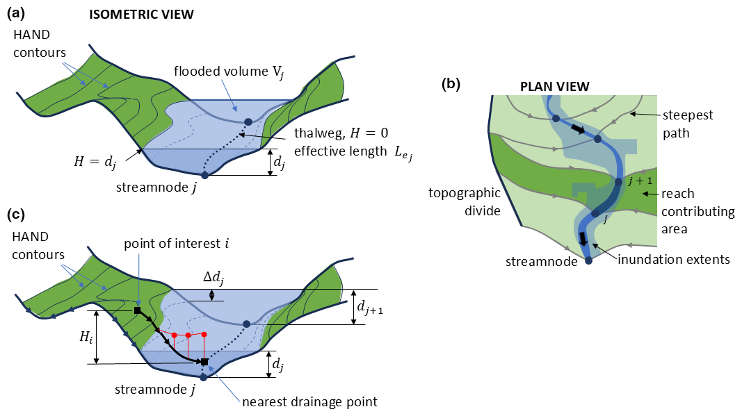
Figure 1 (a) Schematic of a single reach between two streamnodes in pre-processing where the depth is held constant throughout the reach, (b) plan view of the inundated area with the darker green area corresponding to the schematic extents in panel (a), and (c) schematic of the inundated reach with interpolation of depth from streamnodes j and j+1. The water surface elevation is held constant along the red line in panel (c), which is the vertical projection of the drainage path ending in the nearest drainage point.

The flooded area for a given reach is shown schematically in Fig. 1 and provides a representation of how the GASS method discretizes the spatial domain. The figure depicts (a) the view of an inundated reach in pre-processing; (b) the plan view of an inundated reach area delineated by the topographic divide and the steepest path divide at streamnodes; and (c) an inundated reach after the hydraulic model is used to compute depths at each streamnode, and depths are first interpolated between streamnodes and then mapped with a HAND-based method to generate the final inundation map. The terms in the diagram are described throughout this section.

2.2 Hydraulic modelling with the standard step method

In the traditional cross-section approach, the standard step method may be used to compute steady-state depths with gradually varied flow at each streamnode. This method is identical to that used in HEC-RAS (Brunner, 2020).

The standard step method relies on solving Bernoulli's equation without the pressure head term for each pair of streamnodes:

$$\begin{array}{}\text{(1)}& {\displaystyle }{\displaystyle }{z}_j+d_j+{\displaystyle \frac{{\mathit{\alpha }}_{\mathrm{2}}{\overline{v}}_j^{\mathrm{2}}}{\mathrm{2}g}}=z_{j-\mathrm{1}}+d_{j-\mathrm{1}}+{\displaystyle \frac{{\mathit{\alpha }}_{\mathrm{1}}{\overline{v}}_{j-\mathrm{1}}^{\mathrm{2}}}{\mathrm{2}g}}+\mathrm{\Delta }{h}_j,\end{array}$$

where z is the channel invert, d is the channel depth, $\overline{v}$ is the average cross-sectional velocity, α is the velocity coefficient (defined further in Sect. 2.4), g is gravitational acceleration, and h_e is the head loss between two streamnodes. The subscripts refer to the relative location of the streamnode, where j is a given streamnode and j−1 is the downstream streamnode. The Blackbird program currently assumes a subcritical regime, applies a normal depth boundary condition at the downstream-most node (j=1), and then proceeds upstream to solve each streamnode in turn.

The head loss between two streamnodes Δh_j is expressed as

$$\begin{array}{}\text{(2)}& {\displaystyle }{\displaystyle }\mathrm{\Delta }{h}_j=L_{{\mathrm{e}}_j}\overline{S_{{\mathrm{f}}_j}}+C_j\left({\displaystyle \frac{{\mathit{\alpha }}_j{v}_j^{\mathrm{2}}}{\mathrm{2}g}}-{\displaystyle \frac{{\mathit{\alpha }}_{j-\mathrm{1}}{v}_{j-\mathrm{1}}^{\mathrm{2}}}{\mathrm{2}g}}\right),\end{array}$$

where $L_{{\mathrm{e}}_j}$ is the effective stream length, $S_{{\mathrm{f}}_j}$ is the friction slope, and C_j is the expansion or contraction loss coefficient, depending on whether the flow area is larger or smaller than that of the downstream streamnode (A_j). The friction slope is computed at each streamnode using the relationship

$$\begin{array}{}\text{(3)}& {\displaystyle }{\displaystyle }{S}_{{\mathrm{f}}_j}={\left(Q_j/K_j\right)}^{\mathrm{2}},\end{array}$$

where Q_j is the flow rate at the downstream streamnode and K_j is the total conveyance of the streamnode. The average friction slope ${\overline{S}}_{{\mathrm{f}}_j}$ may be computed in a number of ways, where the default in Blackbird is a simple reach average between the downstream and upstream friction slopes. Additional details on the standard step method may be found in Brunner (2020).

While the focus in Blackbird is on the use of reach-integrated hydraulic properties, such as conveyance and cross-sectional flow area (discussed in Sect. 2.4), the expression of hydraulic properties into equivalent form allows properties at streamnodes to be determined from either the traditional cross-section or from reach integration, or a mix of both within the modelling domain, without a change in the standard step solution. This also allows Blackbird to theoretically include any feature of 1D cross-section-based models as well, such as hydraulic structures. This removes a common limitation in large-scale flood mapping applications based on geospatial methods such as the HAND–Manning approach (e.g. McGrath et al., 2018; Chaudhuri et al., 2021), which are unable to handle backwater effects or hydraulic structures.

2.3 Dynamic Height Above Nearest Drainage (DHAND)

In previous studies (e.g. Afshari et al., 2018; Scriven et al., 2021; Chaudhuri et al., 2021; Diehl et al., 2021), the HAND method is used to determine whether a cell is flooded based on its HAND value (H_i) relative to the depth (assumed uniform) in the reach (d_j). A cell is flooded with a depth of d_j−H_i if d_j>H_i. One issue with the processing required to produce a HAND raster is the need to condition the DEM using a breach or fill algorithm prior to computing the HAND raster (e.g. Scriven et al., 2021). This is a common approach in watershed delineation, but in determining flow pathways at a high resolution for flood mapping, this can either create artificial flow pathways that do not exist in the terrain if a breach conditioning algorithm is used or remove storage from the landscape if the fill algorithm is used. This is a known issue with the processing behind the HAND method (Aristizabal et al., 2023), which may lead to artefacts such as false positives in flood maps. In any case, the generation of the HAND raster itself requires manipulating the DEM to determine flow pathways.

The Dynamic Height Above Nearest Drainage (DHAND) is presented here as an alternative to HAND that minimizes the artefacts of terrain alterations through conditioning and is meant to preserve the flow connections in the DEM. This can be of particular importance when natural berms or engineered dykes exist in the landscape. The DHAND algorithm computes a series of raster layers with HAND values as a function of depth, where the number of depth intervals (N_k) and the depth interval between layers (Δd_k) are specified by the user. The calculation of DHAND starts with the initial HAND estimate determined from regular conditioning, which can be considered the DHAND layer for a depth of zero (d_k=0). Then, for each specified depth $d_k=k\cdot \mathrm{\Delta }{d}_k$,

1. a new DEM raster is constructed for the given layer k, where cells with a HAND value H_i of less than d_k in layer d_k−1 are conditioned with a breaching algorithm, which ensures that wetted cells (i.e. cells with H_i<d_k) are connected to the channel and remain wetted – all other cells with H_i≥d_k are conditioned via a fill algorithm, which allows the delineation algorithm to proceed, but ensures that these cells are not artificially breached and connected to the channel for lesser HAND values, and

2. the HAND layer for depth d_k is then computed in the standard way, subtracting the elevation of the cell where a given cell drains to ($z_{i_{\text{min}}}$) from each cell's elevation (z_i) to compute the DHAND layer, i.e. $H_i=z_i-z_{i_{\text{min}}}$.

The algorithm is described graphically in Fig. 2. This use of conditional breaching and filling of the DEM allows the landscape connections to be largely preserved and particularly ensures that cells at lower elevations do not artificially become inundated for a given depth because of the conditioning algorithm. The accuracy of this method is improved with higher-resolution depths applied in DHAND, at the cost of additional pre-processing and storage requirements, as each depth produces a new raster DHAND layer. The effect of this processing is shown graphically in Fig. 3.

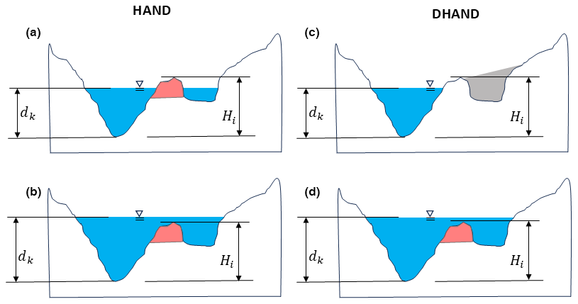
Figure 2 The DHAND algorithm is described graphically in profile view, contrasting HAND and DHAND. With HAND, all cells are typically breached (red areas) in conditioning the DEM, leading to the embedded assumption that low-lying areas are hydraulically connected in all cases (a and b). With DHAND, the low-lying area is filled (grey areas) when the depths are low (c) and only becomes wetted (d) when depth d_k exceeds the HAND value of the berm (H_i).

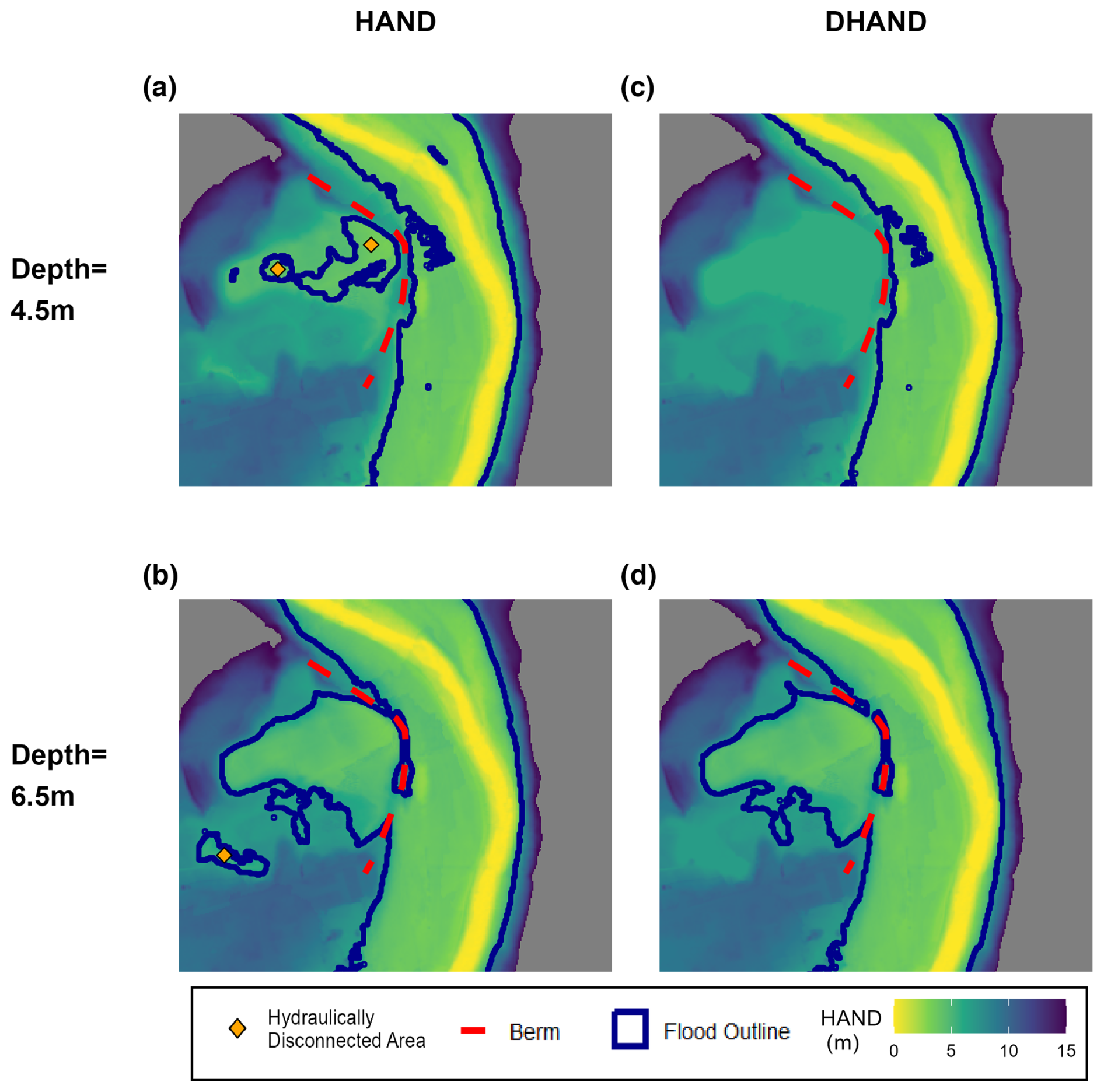
Figure 3 HAND and DHAND layers are applied for fixed depths to compute flood extents adjacent to a river bend. (a) HAND layer with shallower depth of 4.5 m shows flooding in two hydraulically disconnected areas on the inside of a berm. (b) Same HAND layer from panel (a) with a greater depth of 6.5 m shows greater flooding inside the berm area as it is overtopped and also shows a new disconnected and inundated area that appears down and left of the original area. (c) A DHAND layer for the specific depth of 4.5 m shows no flooding on the other side of the high berm. (d) The DHAND layer for a depth of 6.5 m now allows flooding on the other side of the berm as it is overtopped and does not generate falsely inundated areas as with the HAND layer in panel (b). These scenarios also correspond to the panels of Fig. 2.

2.4 Reach-integrated hydraulic properties

The depth in each cell (d_i) is determined by comparing the 1D reach-integrated depth d_j to the DHAND value of the raster cell (H_i). This assumes a flat raster cell where slope and aspect are neglected. The depth in each cell is calculated as $d_i=max(d_j-H_i,\mathrm{0})$.

The flooded area (A_i) is a binary function, defined as

$$\begin{array}{}\text{(4)}& {\displaystyle }{\displaystyle }{A}_i=\left\{\begin{array}{ll}\mathrm{0}& \text{ if }{d}_i=\mathrm{0}\\ A_i& \text{ if }{d}_i>\mathrm{0},\end{array}\right.\end{array}$$

where a is the square raster cell dimension. Similarly, the flooded volume V_i is computed as $V_i=A_i\cdot d_i$ if the ith cell is inundated, and it is zero otherwise. The effect of slope being incorporated into these equations was tested and found to have a negligible impact on results, and thus the simpler equations are adopted in calculating area and volume for raster cells.

In a traditional cross-section-based 1D model, we compute conveyance in each section of the cross-sectional flow area as

$$\begin{array}{}\text{(5)}& {\displaystyle }{\displaystyle }{K}_b={\displaystyle \frac{\mathrm{1}}{n_b}}{A}_b{R}_b^{\mathrm{2}/\mathrm{3}},\end{array}$$

where K_b is the conveyance of the bth section, n_b is Manning's roughness, A_b is the flow area, and R_b is the hydraulic radius, computed as $A_b/P_b$, where P_b is the wetted perimeter.

To compute the total conveyance in a cross-sectional model, we can sum the conveyance in each section:

$$\begin{array}{}\text{(6)}& {\displaystyle }{\displaystyle }{K}_j=\sum _{b=\mathrm{1}}^{N_b}{K}_b,\end{array}$$

where K_j is the total conveyance of the cross-section, and N_b is the number of sections (or slices) within the cross-section. The number of sections or slices is typically based on the number of ordinates (i.e. each pair of x, z coordinates constitutes a new section) or the sections are grouped based on whether the roughness value changes, which results in fewer sections.

In the reach-integrated approach we consider each raster cell as a section and substitute N_b sections for N_i cells. We further substitute the cross-sectional flow area for total cell flooded volume V_i and the cross-sectional wetted perimeter for the total cell flooded area A_i. The term is then divided by the effective length of the reach, $L_{{\mathrm{e}}_j}$, which creates a term that is comparable to that traditionally computed for a cross-section. This approach is similar to that of Zheng et al. (2018b), though we use the effective length rather than reach length, as the effective reach length is more representative of the flow path as a function of depth than a static reach length. This is written as

$$\begin{array}{}\text{(7)}& {\displaystyle }{\displaystyle }{K}_j={\displaystyle \frac{\mathrm{1}}{L_{{\mathrm{e}}_j}}}\sum _{i=\mathrm{1}}^{N_i}{K}_i={\displaystyle \frac{\mathrm{1}}{L_{{\mathrm{e}}_j}}}\sum _{i=\mathrm{1}}^N{\displaystyle \frac{\mathrm{1}}{n_i}}{V}_i{R}_i^{\mathrm{2}/\mathrm{3}},\end{array}$$

where in the reach-integrated set of properties, $R_i=V_i/A_i$, which is analogous to $A/P$ in the original Manning equation and equivalent in a uniform channel cross-section. We can similarly compute reach-integrated area and wetted perimeter, and we compute the flow area of the jth streamnode (A_j) as

$$\begin{array}{}\text{(8)}& {\displaystyle }{\displaystyle }{A}_j={\displaystyle \frac{\mathrm{1}}{L_{{\mathrm{e}}_j}}}\sum _{i=\mathrm{1}}^{N_i}{V}_i\end{array}$$

and the wetted perimeter (P_j) of the jth streamnode as

$$\begin{array}{}\text{(9)}& {\displaystyle }{\displaystyle }{P}_j={\displaystyle \frac{\mathrm{1}}{L_{{\mathrm{e}}_j}}}\sum _{i=\mathrm{1}}^{N_i}{A}_i.\end{array}$$

The effective reach length of the channel is intended to capture the distance travelled by water from one point to another and is then used to determine energy losses incurred by that travel. In traditional 1D models, this is resolved by inputting the main, left, and right channel distance manually (N_b=3) and often by using a flow-weighted arithmetic mean to determine the effective length for energy loss. In the cross-section-based implementation of our model, we use a similar conveyance-weighted approach to determine effective reach length:

$$\begin{array}{}\text{(10)}& {\displaystyle }{\displaystyle }{L}_{{\mathrm{e}}_j}={\displaystyle \frac{\mathrm{1}}{K_j}}\sum _{b=\mathrm{1}}^{N_b}{L}_b\cdot K_b,\end{array}$$

where N_b=3 and represents the left, right, and main channel sections.

In the reach-integrated implementation, we aim to determine the effective reach length automatically based on the geospatial data available without the need to prescribe the channel lengths for three locations (left, main, right), as is traditionally done in the cross-section approach. Instead, we compute a reach-length raster input, which determines the mean travel path length within the reach for a given stage. Conceptually, this reach-length raster represents the average path length that a droplet of water, if travelling through the reach at the given location and elevation of the raster cell it is located on, would travel from the upstream boundary of the reach to the downstream boundary of the reach. Within the channel this is determined from the channel vector polyline, and elsewhere this is determined from contour lines derived from the HAND raster. The path lengths mapped as a set of polylines are then interpolated to the DEM resolution to generate the reach-length raster.

The effective reach length ($L_{{\mathrm{e}}_j}$) of the jth streamnode for a specific depth is computed as

$$\begin{array}{}\text{(11)}& {\displaystyle }{\displaystyle }{L}_{{\mathrm{e}}_j}={\displaystyle \frac{\mathrm{1}}{{\sum }_{i=\mathrm{1}}^{N_i}{K}_i}}\sum _{i=\mathrm{1}}^{N_{\text{cells}}}{L}_i\cdot K_i,\end{array}$$

where L_i is the estimated reach length in the ith cell (determined from the reach-length raster), and K_i is the cell conveyance.

Two other terms that need to be computed in order to facilitate steady-state hydraulic calculations include the alpha term (α), which is a correction to the average velocity, and the composite Manning n (n_c).

The alpha term (α) accounts for the underestimation of mean velocity when computed from the sum of individual components. This value is generally between 1.0 and 4.7 (Hulsing et al., 1966). In a cross-section approach, the alpha term has been computed as (Brunner, 2020)

$$\begin{array}{}\text{(12)}& {\displaystyle }{\displaystyle }{\mathit{\alpha }}_j={\displaystyle \frac{A_j^{\mathrm{3}}}{K_j^{\mathrm{2}}}}\left(\sum _{b=\mathrm{1}}^{N_b}{\displaystyle \frac{K_b^{\mathrm{3}}}{A_b^{\mathrm{2}}}}.\right).\end{array}$$

We compute α_j in the same manner with the catchment approach, noting that the conveyance K_b is now the conveyance of an entire cell (K_i), and the cross-sectional area A_b is replaced by the total flooded volume of the cell V_i. This substitution is valid because the effective length term $L_{{\mathrm{e}}_j}$ appears in the numerator and denominator in converting cross-section properties to reach-integrated properties and is thus cancelled out. This can be written as follows:

$$\begin{array}{}\text{(13)}& {\displaystyle }{\displaystyle }\mathit{\alpha }={\displaystyle \frac{V_j^{f\mathrm{3}}}{K_j^{\mathrm{2}}}}\left(\sum _{i=\mathrm{1}}^{N_i}{\displaystyle \frac{K_i^{\mathrm{3}}}{V_i^{f\mathrm{2}}}}\right).\end{array}$$

The composite Manning n in the cross-sectional approach (n_c) can be computed using one of many equations (see Chow, 1959, Eqs. 6–17 through 6–19), including the equal force equation, equal velocity, weighted average conveyance, weighted average area, and others. No single method has been deemed the most appropriate in the literature. Here, we again substitute the cross-sectional area with the flooded volume and substitute the cross-sectional wetted perimeter with the flooded cell area. The default composite Manning n estimation approach in Blackbird is the equal velocity method, which can be written in reach-integrated form as

$$\begin{array}{}\text{(14)}& {\displaystyle }{\displaystyle }{n}_c={\left({\displaystyle \frac{{\sum }_{i=\mathrm{1}}^{N_i}{A}_i{n}_i^{\mathrm{1.5}}}{A_j}}\right)}^{\mathrm{2}/\mathrm{3}}.\end{array}$$

2.5 Post-processing and flood map generation

Following the execution of the hydraulic model calculations with a standard step approach, the mapping of hydraulic results at each streamnode is performed to generate a flood map of depths and/or inundation extents. The typical approach with HAND is to apply the reach-integrated depths d_j within each reach and compute depths in each cell as $d_i=max(d_j-H_i,\mathrm{0})$.

In Blackbird, the thalweg depths are first interpolated along the reach, reducing the occurrence of sharp differences in depths within the flood map. This creates a series of interpolated depths ${\widehat{d}}_j$ along the reach, where $d_j\le {\widehat{d}}_j\le d_{j+\mathrm{1}}$. The interpolated depths ${\widehat{d}}_j$ may optionally be corrected with the term $({\widehat{z}}_t-z_t)\cdot C_t$ to take into account the variability of the DEM elevations at the thalweg, such that the final water surface elevation remains a smooth linearly interpolated grade between streamnodes j and j+1 rather than a water surface that reflects the variability of bed elevation in the channel. The interpolated depths ${\widehat{d}}_j$ are computed as

$$\begin{array}{}\text{(15)}& {\displaystyle }{\displaystyle }{\widehat{d}}_j=d_j+(d_{j+\mathrm{1}}-d_j)\cdot {\displaystyle \frac{{\widehat{L}}_j}{L_{{\mathrm{e}}_j}}}+({\widehat{z}}_t-z_t),\end{array}$$

where ${\widehat{L}}_j$ is the length of the thalweg from streamnode j to the nearest drainage point associated with ${\widehat{d}}_j$, ${\widehat{z}}_t$ is the linearly interpolated channel bed elevation, and z_t is the actual bed elevation (i.e. thalweg elevation). Where the depths are corrected by thalweg elevation in post-processing, the same correction would be applied in pre-processing hydraulic properties for consistency.

The depths in each cell (d_i) are then computed using the closest DHAND information corresponding to the interpolated depth ${\widehat{d}}_j$, and depths in each cell are computed as $d_i=max({\widehat{d}}_j-H_i,\mathrm{0})$. Blackbird supports the use of DHAND or HAND for the post-processing step of map generation, as well as the options to interpolate depths or apply the depth uniformly within the reach.

2.6 Evaluation metrics

Several key metrics are used to evaluate model quality against either a benchmark model or flood polygons. If a benchmark model result with depths in each cell is available as the observed data set, error metrics based on the difference in depths between cells may be computed. Here, we use the mean absolute error (MAE), computed as

$$\begin{array}{}\text{(16)}& {\displaystyle }{\displaystyle }\text{MAE}={\displaystyle \frac{\mathrm{1}}{N_m}}\sum _{m=\mathrm{1}}^{N_m}|d_m^{\mathrm{s}}-d_m^{\mathrm{o}}|,\end{array}$$

where N_m is the total number of cells evaluated (typically, all cells within a defined boundary), $d_m^{\mathrm{s}}$ represents the simulated depth in the mth cell, and $d_m^{\mathrm{o}}$ represents the observed depth (noting that here we treat modelled depths from the 2D model as observed). The range for this metric is [0,∞], where 0 is an ideal score.

The other metrics used herein are Matthew's correlation coefficient (MCC) and the error bias (B), both of which are commonly used in image processing applications to assess binary classification accuracy. The MCC is considered to be the most informative metric within this domain (Chicco, 2017). The MCC is computed as

$${\displaystyle }\text{MCC}={\displaystyle \frac{\text{TP}\cdot \text{TN}-\text{FP}\cdot \text{FN}}{\sqrt{(\text{TP}+\text{FP})\cdot (\text{TP}+\text{FN})\cdot (\text{TN}+\text{FP})\cdot (\text{TN}+\text{FN})}}},$$

where TP is a true positive, TN is the true negative, FP is a false positive, and FN is a false negative. The range for MCC is $[-\mathrm{1},\mathrm{1}]$, where −1 indicates that no cells were correctly classified, 0 indicates equal performance to random chance, and 1 indicates a perfect classification of cells.

We also compute the error bias B as defined in McGrath et al. (2018):

$${\displaystyle }B={\displaystyle \frac{\text{TP}+\text{TN}+\text{FP}}{\text{TP}+\text{TN}+\text{FN}}},$$

where a value of 1 is ideal and indicates no bias, while $\mathrm{0}\le B<\mathrm{1}$ indicates a tendency towards underprediction, and $\mathrm{1}<B<\mathrm{\infty }$ indicates a tendency towards overprediction.

2.7 Case studies

We present a verification test and an applied case study of the Blackbird approach. First, we provide the simple verification benchmark tests, which are comprised of a set of six test cases (SB01–SB06), which are intended to verify the ability of Blackbird to provide a steady-state solution using the standard step method with cross-sections before it is used in the reach-integrated configurations. We deploy HEC-RAS 1D and Blackbird to both model sets of cross-section data without any reach integration or other novel methods presented in this paper.

The second case study is based on a physical location near the community of Waldemar, Ontario, within the Grand River watershed. The base terrain is based on high-resolution bathymetric and topographic data to ensure representation of the channel and floodplain geometries. In this case study we apply a fully 2D quasi-steady-state model in HEC-RAS, which is treated as the truth and used as the point of comparison for the 1D-based approaches. The purpose of this case study is to compare the HAND–Manning method, a cross-section-based 1D model in HEC-RAS 1D, and the Blackbird model in their ability to approximate the results from the fully 2D model. The model results for both uncalibrated and calibrated models are provided.

The HAND–Manning method is also implemented within the Blackbird software and uses the reach-integrated estimation of hydraulic properties from a HAND raster that is otherwise consistent with the Blackbird methodology. The normal depth in each streamnode is then estimated using Manning's equation to determine depth, providing the reach-integrated bed slope as the slope term. The depth results are generated for each streamnode and combined to create a flood map. The HEC-RAS 1D model refers to a fully 1D model built with HEC-RAS software offered by the US Army Corps of Engineers (Brunner, 2020). The same software is used to interpolate results between cross-sections and generate flood maps.

2.7.1 Simple verification benchmarks

In the simple verification benchmark tests, we deploy six basic tests in comparing cross-section-based models to ensure that the Blackbird standard step approach is consistent with industry-standard software. We apply the following tests in order of increasing complexity:

1. SB01 – basic trapezoidal channel with symmetric roughness values in the left, channel, and right banks, and consistent length values of 50 m in the left, channel, and right banks;

2. SB02 – basic trapezoidal channel with asymmetric roughness values (higher roughness in one bank than the other);

3. SB03 – basic trapezoidal channel, asymmetric roughness values, and asymmetric and varying channel lengths in banks;

4. SB04 – basic trapezoidal channel, varying channel lengths in banks, and horizontally varying roughness values as a vector rather than specifying three roughness values for the left, channel, and right banks;

5. SB05 – basic trapezoidal channels on three reaches, asymmetric roughness values, asymmetric and varying channel lengths in banks, and a junction; and

6. SB06 – 49 realistic cross-sections cut from real terrain data along a single channel with horizontally varying roughness values.

The last test, SB06, uses the sections and setup from the Waldemar 1D case study (described in the following section) under the high-flow scenario. These six tests are used as a verification of the ability of Blackbird to correctly compute steady-state subcritical hydraulic results as a necessary check before deploying those algorithms for more complex application. Each set of results uses the depth at each cross-section to verify the agreement of the models.

2.7.2 Waldemar

This case study is developed as a test bed to compare the various modelling approaches against the results of a 2D hydraulic model (built using HEC-RAS 2D). The philosophical approach taken here is to consider the 2D model as observed or truth data, with the goal of the simplified modelling approaches being to approximate the 2D model as closely as possible.

The town of Waldemar is located along the Grand River in Ontario, Canada, approximately 14 km west of Orangeville. The Grand River flows from the north through the town of Grand Valley, meanders, and then flows through the town of Waldemar. The extents of the case study are depicted in Fig. 4. The terrain was generated from a combination of the Southwestern Ontario Orthophotography Project 2020 (SWOOP2020) data product and bathymetry data provided by the Grand River Conservation Authority (GRCA). The SWOOP2020 product is freely available at a 0.5 m resolution across all of southwestern Ontario, including the Waldemar study area, and is offered under the Open Government License – Ontario. The bathymetry data were provided as a point cloud file under the GRCA Open Data License v2.0. The bathymetry data were processed into a 0.5 m DEM using the lidR package in R (Roussel et al., 2020; Roussel and Auty, 2024). These products were merged into a single terrain file at a 2 m resolution to capture both bathymetry and terrain elevations. Land cover data were obtained from the GRCA Land Cover 2017 product (also available under GRCA Open Data License v2.0) and reclassified to Manning's n roughness values using standard values from Chow (1959).

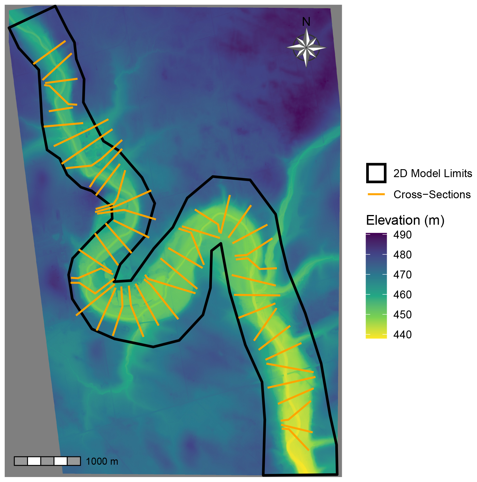
Figure 4 Location of the case study in the town of Waldemar. The extents of the HEC-RAS 2D model and the cross-sections from the HEC-RAS 1D model are shown.

The flows provided to the model were derived from a flood frequency analysis on annual peak daily flow data obtained from Water Survey of Canada gauge 02GA014. The data were corrected by a drainage ratio to the location of historic gauge 02GA022 located within the study area and then analyzed for extremes by fitting to the generalized extreme value distribution using the extRemes package in R (Gilleland and Katz, 2016). The flows used in this case study were 156.2 m³ s⁻¹ (low flow), 246.4 m³ s⁻¹ (medium flow), and 314.7 m³ s⁻¹ (high flow), which correspond to return periods of approximately 2-, 10-, and 100-year flows (50 %, 10 %, and 1 % annual exceedance probabilities), respectively. Only flows along the Grand River were considered in this model benchmark, though other tributaries exist within the study area.

The HAND–Manning, HEC-RAS 1D, HEC-RAS 2D, and Blackbird models are compared within the Waldemar case study. All four models used the same terrain, land cover, and flow inputs. Fifty cross-sections for the HEC-RAS 1D model were cut over the 13.5 km domain and adjusted to avoid overlapping in meanders. The cross-section thalweg locations were used as streamnode locations for the HAND–Manning and Blackbird models. Terrain and roughness data for the HEC-RAS 1D model were obtained from the raster inputs using native HEC-RAS tools to populate cross-section data. Bridges are present at crossings in the area but are omitted in all models here for simplicity. The roughness values in all non-2D models were initially multiplied by a single roughness multiplier of 1.1 in recognition that the losses encapsulated by the roughness term vary based on the modelling approach (Morvan et al., 2008) and are generally higher in more simplified models where more energy losses are abstracted by the roughness coefficient rather than defined in the mathematical formulation. The initial uncalibrated factor of 1.1 was determined by comparing depths in key sections of the HEC-RAS 1D and 2D models and adjusting the global roughness multiplier until the error in depths at those sections was minimized. The roughness multiplier was later calibrated manually for each of the three benchmarked models using the NSSE scores to develop calibrated models.

In developing the 2D hydraulic model with HEC-RAS 2D, a base cell resolution of 5 m was used with additional refinement along the main channel and hydraulic features in the model, such as berms and ponds. The model was run in unsteady mode using the shallow-water equations Eulerian–Lagrangian method (SWE-ELM) method. The conservative turbulence model was also included to account for turbulent effects. The time step was configured as an adaptive time step, with an initial time step of 0.5 s and allowing a range of 0.016 to 4 s time steps. The maximum depth error (as reported by the HEC-RAS solver) across all three flow simulations was found to be less than 0.23 m in water surface elevation, with an overall volume accounting error of 0.0047 % or less in each run. The model runtime was between 2–4.5 h per run on an i9 desktop with 24 cores, depending on the flow scenario. The HAND–Manning and Blackbird models required a pre-processing runtime of approximately 70 min to compute hydraulic properties prior to the model runs. The model runtime of a few seconds was negligible in comparison and is similar to the runtime in HEC-RAS 1D. The generation of result rasters using any approach ranged from 30–120 s.

3 Results

3.1 Simple verification benchmarks

The results from the simple benchmark tests found that in case studies SB01–SB05, the Blackbird algorithm had a maximum error in depth of 1 cm (translating to approximately 0.08 % error in depth), which was found on a few sections and is likely due to small numerical errors or rounding to the nearest centimetre. Aside from that, the HEC-RAS 1D results are effectively emulated by the Blackbird code for these simple tests.

In SB06, the full complexity of model inputs derived from real data, including up to 500 ordinates per cross-section, was introduced. This is unlike the theoretical cross-sections and hydraulic parameters used in SB01–SB05. The maximum error in SB06 was bounded by ±0.2 m (t-test p value of 0.315), which is approximately ±5.25 %. Based on the results of a t test on the mean and Shapiro–Wilk test, respectively, the mean of the data is not significantly different from zero and appears to be normally distributed. A plot of the errors is provided in Fig. 5, indicating that the errors appear homoscedastic and normally distributed. The errors in SB06 may be due to aggregated rounding errors in each cross-section, as the modelled cross-sections have between 175 and 500 points each, while earlier experiments had only eight (8) points per cross-section. There may be other differences in the algorithms as well, such as in the algorithmic handling of inundated areas outside of the main channel or other nuances that were not represented in SB01–SB05.

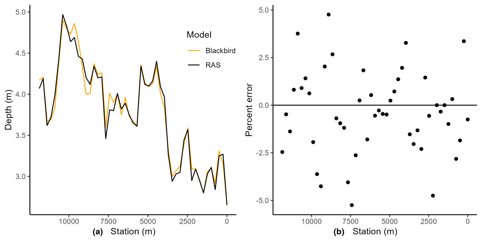
Figure 5 Results of the SB06 benchmark test, summarized with a profile plot for both Blackbird and HEC-RAS generated results (a) and the residual depth errors shown (b). Errors are bounded by ±0.2 m and are randomly distributed around a mean of zero.

Overall, the simple benchmark results indicate that the Blackbird code is working as expected when deploying the standard step method in subcritical regimes for a set of cross-sections when compared to HEC-RAS 1D. The code is able to replicate the results of simple case studies almost exactly and with a small amount of error in a very complex terrain. This provides sufficient confidence for using the code in the reach-integrated application, which is the focus of this study.

3.2 Waldemar

The metrics (defined in Sect. 2.6) were computed for each scenario in the Waldemar case study and are provided in Fig. 6. The evaluation is based on all raster cells within a defined evaluation area, and for each flow regime (low, medium, or high), any cells that are consistently dry in all model results are removed from the calculation of metrics. This pruning of dry cells does not impact the relative ranking of models in the results. The results indicate that based on all metrics, the best model in each flow scenario was consistently Blackbird, followed by HEC-RAS 1D and then HAND–Manning.

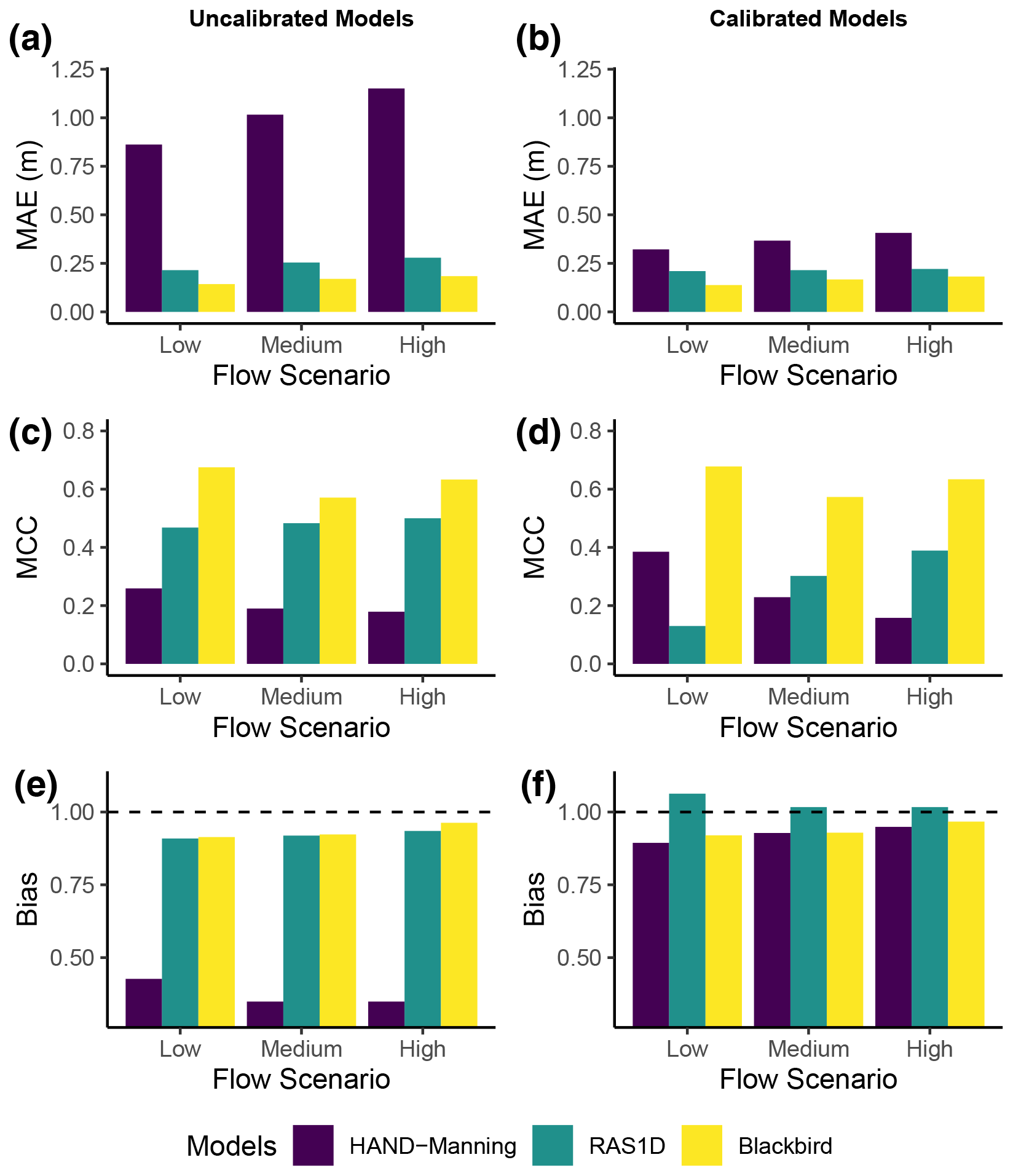
Figure 6 Results for the three model runs evaluated against the HEC-RAS 2D model under three flow scenarios. All raster cells within a defined evaluation area were evaluated, and cells that were not consistently dry in all four models (including the 2D model) were used in the calculation of metrics. Metrics used are the mean absolute error (MAE), Matthew's correlation coefficient (MCC), and the error bias. Plots (a), (c), and (e) show uncalibrated model results, and plots (b), (d), and (f) show calibrated model results. Ideal values for MAE, MCC, and bias metrics are 0.0, 1.0, and 1.0, respectively.

The HAND–Manning method is generally ranked last in performance, with errors substantially larger than other methods, particularly when examining the MAE results. The depths generated by HAND–Manning methods are always underestimated in this case study, particularly when uncalibrated (see Fig. 6e), and require calibration to increase roughness by a large factor in order to approach reasonable results. This in particular highlights the value added by considering energy losses via a hydraulic model rather than performing geospatial-based analysis alone, as the energy loss impacts are substantial.

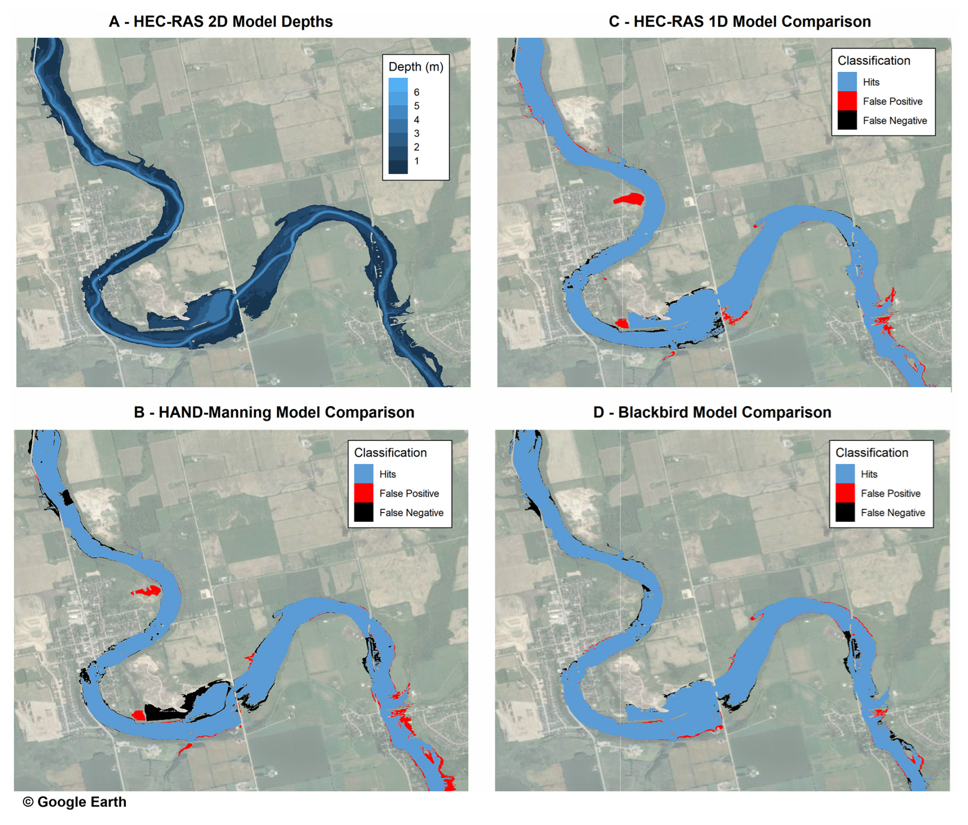
Figure 7 Calibrated model results compared against 2D model results, showing the results for (a) the HEC-RAS 2D model depths, (b) the HAND–Manning model classified differences, (c) classified differences for the HEC-RAS 1D model, and (d) classified differences for the Blackbird model output.

Results were generally improved by calibration, though the HAND–Manning method was substantially improved, and the Blackbird results were only marginally improved as the initial roughness multiplier was almost unchanged. The HEC-RAS1D models improved in MAE but worsened in MCC when calibrated. This is due to the calibration to a depth-based metric, which resulted in improved MAE scores but also generated additional false positives in the HEC-RAS1D model results, decreasing the MCC score. The calibrated roughness multiplication factors were 4.83, 1.35, and 1.14 for the HAND–Manning, HEC-RAS1D, and Blackbird methods, respectively (compared to an initial multiplier of 1.1). The difference in roughness multipliers highlights the drastic need to compensate for a lack of inherent energy losses in the HAND–Manning method. The difference in calibrated multipliers between the HEC-RAS 1D and Blackbird models also suggests that there may be additional energy losses captured with the reach-integrated approach relative to the cross-section approach, leading to the lower multiplier in the Blackbird model.

The model results were visually compared to the 2D model results in Fig. 7 to show locations where the inundated (wetted) and dry areas varied from the 2D output. Outputs were mapped in a categorical classification scheme to show where results were (1) accurately classified as wetted (hits); (2) false positives, where the model produced a wetted cell in a cell with no water from the 2D model; and (3) false negatives, where a dry well was produced where the 2D model was wetted.

Figure 7 shows clearly how the HAND–Manning method has the largest swaths of both false-positive and false-negative areas. The area on the inside bend near the northern part of the study area is wetted (false positive) in both the HAND–Manning and HEC-RAS 1D results though not in the Blackbird results – a phenomenon which is further explained by Fig. 3. While some areas of both false positives and false negatives exist in all three model results, the Blackbird model is successful in minimizing the large areas of false positives due to channel connection issues or due to resolving the threshold at which the channel spills to a low-lying area. This can be attributed to a combination of accurate depth estimations as well as the DHAND method used to resolve spatial connections on the landscape.

4 Discussion

4.1 Inundation forecasting requirements

Computational runtime is an important consideration both in large-scale and forecasting applications, where obtaining accurate model results in a timely fashion is critical. This may be compounded if any model calibration or uncertainty analysis requires the model to be run hundreds or thousands of times in a short time frame, and potentially without the computing resources necessary to run 2D models quickly.

A key benefit of Blackbird is that the computationally expensive estimation of hydraulic properties is handled in pre-processing, leaving the remaining simulation runtimes to be essentially equivalent to that of any 1D model. For instance, in the Waldemar case study the simulation runtime of the HEC-RAS 2D model runtime was 4.5 h for the high-flow scenario while the Blackbird runtime was less than a few seconds, which is approximately ×10 000 faster. This difference in runtime is similar to that of a 1D HEC-RAS model. This difference in model runtime can be expected to increase substantially with studies of a larger extent. It is also worth noting that the same pre-processing is required for the HAND–Manning method as Blackbird; thus, despite the simplicity of the HAND–Manning technique the computational-cost savings are negligible.

A feasible current practice for estimating flood extents in real-time forecasting applications is through the use of existing flood maps. Agencies responsible for flood forecasting will typically possess maps of estimated flood extents for potential floods with a specific probability, defined by an annual return period or exceedance probability. For example, a forecaster may access maps showing the flood extents of the 1-in-50-year and 1-in-100-year floods for an area of interest. A real-time flow estimate may coincide with a 1-in-80-year return period, in which case the two maps for the 50- and 100-year extents would be used to estimate flood extents of the current event. However, complications arise in this kind of interpretation that can render this exercise very challenging. For example, the maps may be out of date in either the estimated probabilities of flows, the landscape information, or the methodologies which produced the maps, leading to complications in easily interpreting flood maps under the pressure of issuing forecasts and decisions in real time. At junctions, the pre-computed flood maps for specific likelihoods are often made with idealized scenarios regarding the timing of peak flows or equal probability of flows at both upstream sections of the junction (e.g. 100-year flow on each branch). However, in practice there will likely be a different probability determined for the flows on each branch, such as a 1-in-80-year flow on one branch and 1-in-130-year flow on the second branch, making the use of a set of pre-computed flood maps less useful. There may also be backwater effects impacting flooding due to major constrictions on the channel downstream of the area of interest, which may not have been considered in the generation of the pre-computed maps. In these scenarios the pre-computed flood maps are far less useful to forecasters and decision-makers than a model which can be run in real time. Inundation forecasting, i.e. issuing forecasts of flood depths at specific locations, is much less common today than streamflow forecasting but may be supported by the capabilities of Blackbird to address many of the above issues and support accurate inundation maps in real time.

4.2 Relative model development effort

Another important consideration in developing models is the relative effort requiring manual intervention. While software exists to generate cross-sections automatically and populate the necessary data such as bank stations and channel lengths, manual intervention is often required to avoid overlapping cross-sections at meanders and generally to ensure a proper representation of the channel and floodplain via cross-sections. In addition, special attention must be given to the location of cross-sections along the channel profile and ensuring that sections are consistently placed at the top of riffles or other consistent features within the profile. Inconsistent placement of sections along the profile can lead to a poor definition of the channel inverts solely as a result of cross-section placement. Two-dimensional models also involve a fair amount of manual work, particularly in defining the breaklines during mesh generation, which are required to avoid artificial spilling of water across cells.

By contrast, Blackbird simplifies much of the effort to a set of automated functions, and the only manual labour is the same quality assurance required for any modelling exercise. For example, cross-sections do not need to be cut; only point locations for computational nodes need to be defined, which can be done automatically and are theoretically less sensitive to placement along the channel profile than cross-sections because of the reach-integration approach. Contributing area extents are defined by catchment areas around each streamnode. These still require checking but are generated automatically and are therefore less prone to error and bias by a modeller, such as extending a cross-section short of the potential flood extent. Bank stations and reach lengths are not explicitly defined in the Blackbird configuration as they are in HEC-RAS 1D, as bank stations are not used and reach lengths are calculated dynamically. Overall, the degree of manual effort is greatly reduced in the development of a Blackbird model relative to the traditional cross-section-based 1D model or fully 2D models.

4.3 Modelling challenges and limitations

The popularity of HAND-based flood maps has increased in recent years, which is likely driven by the ease of implementing the method as well as the low computational requirements. Validation of HAND-based models is often presented as adequate when the HAND-generated flood map captures some of the flood extents derived from satellite imagery (e.g. Scriven et al., 2021; Chaudhuri et al., 2021) or in comparison to other even simpler methods (e.g. McGrath et al., 2018). However, the limitations of this method are sometimes downplayed and warrant further discussion. The HAND–Manning method applies Manning's equation for depth estimation in each defined reach independently, and thus depths may vary substantially between reaches without any impact on adjacent reaches. The HAND–Manning method is noted to underperform in certain environments, such as meandering portions of channels or near hydraulic structures (Afshari et al., 2018), and is considered by Jafarzadegan et al. (2023) to only work in confined floodplains. The inability of the HAND–Manning method to incorporate energy losses, hydraulic structures, ice jams, or backwater effects is also severely limiting, as shown partially by the results of this study. While idealized conditions may be encountered, often the events that cause severe flooding are related to one or more of these hydraulic conditions (i.e. high energy losses, backwater effects from a downstream constriction, obstructions at bridges or culverts, ice jams, etc.). A model that is validated under idealized flows and then applied to forecast or simulate a real flood event under one of the aforementioned conditions may result in severe underprediction of depths with potentially disastrous consequences.

In comparing Blackbird with HEC-RAS 1D, the models are fundamentally similar in the computation because of the exact same underlying sets of equations and solvers (under steady-state conditions). Where the models differ is in the landscape discretization and representation within the model. Theoretically, the GASS method uses more of the available information in determining hydraulic properties than a cross-section approach, which discards the majority of data available to the modeller. It is unlikely that there would be scenarios in which GASS would underperform the cross-section methodology under the same set of input data. The scenarios where this may not be true are primarily related to the underlying catchment delineation algorithm used to define reach areas, such as very flat areas where catchment delineation is a challenge or other scenarios where the reach-integration approach is not a fair reflection of the hydraulic conditions. However, the ability of Blackbird to also represent streamnode properties with cross-sections alleviates any limitations relative to the cross-section approach, and future developments planned for Blackbird (such as representing hydraulic structures) will likely remove this relative limitation altogether. Other challenges of 1D modelling, such as conditionally varying or ephemeral flow paths (i.e. flow paths that may short-circuit the channel for some depths), are a challenge for both Blackbird and HEC-RAS 1D, since both of these models require a defined static channel line. Such cases are currently best handled with 2D models.

The Blackbird and HEC-RAS 1D models presented here are both steady-state models, which assume that flow values are sustained for a sufficient amount of time for steady-state conditions to be achieved. In practice, this is a conservative assumption compared to unsteady state where a time series of flows is provided rather than a fixed peak value. Under unsteady flow, the volume of water provided by the flow boundary conditions is taken into account in the hydraulic modelling. This can be particularly important in low-slope or flat areas where a small change in average depth of a cross-section of streamnode can result in vastly greater volumes of water on the landscape. As a check in the Waldemar case study, the cross-sectional flow area in each reach-integrated streamnode can be multiplied by the effective reach length and summed to get the total volume of water in the modelled landscape. Dividing this by the flow and converting units reveals a time period of approximately 3.5 h, which is conceptually the duration that the given flow rate would need to be maintained in order to deliver enough water to the system to fill the landscape (including floodplains) to the modelled extents. In the Waldemar example, a large proportion of this storage comes from a single streamnode where an offline storage pond is found and assumed initially dry in this model. This type of check on the system is important particularly when the landscape is flat, which can lead to overly conservative estimates of flood extents, and this duration check can reveal whether the steady-state assumption over the entire domain is a reasonable one. Future testing of Blackbird in case studies with varying terrains, including high slopes and flat areas, will show how the method and software performs in less ideal circumstances.

4.4 Future development

Future developments are planned to expand the capabilities of the Blackbird software. Further testing would involve fully understanding under which conditions the GASS approach performs well and where it does not, as well as what modifications may be required to address those limitations. Additional testing for features that are implemented though not studied in this work includes the modelling of junctions, as well as a mixed representation of streamnodes as cross-sections and reach-integrated properties within a modelling domain.

Additional features that are not yet implemented include the ability to represent hydraulic structures, such as bridges and culverts, which are very commonly encountered in systems with potential to impact humans under flood conditions. The development of hydraulic structures will take two approaches: (1) implementing hydraulic structures with cross-section-based streamnodes akin to what is done in HEC-RAS 1D and (2) more abstract reductions in flow area at streamnodes, which would be less accurate but have fewer data requirements. The latter in particular is intended to support modelling at large scales, where the presence of hydraulic structures can be detected at road crossings through geospatial analysis, but detailed survey information may not be available.

Another planned extension is the inclusion of unsteady flow (i.e. 1D Saint-Venant equations) to support time-varying hydrographs as boundary conditions. As discussed in Sect. 4.3, the steady-state assumption may be overly conservative, especially in flat areas, and lead to an overestimation of flood risk. This can be addressed by the use of unsteady-flow solutions. The inclusion of ice jams is also a possible extension to Blackbird capabilities. As with hydraulic structures, ice jams could be represented either with a cross-section approach as is done in HEC-RAS 1D or with a more generalized reach-integrated approach that reduces the flow area and increases resistance to flow in particular streamnodes. The latter may be more promising as the locations and properties of ice jams are often a source of great uncertainty, and thus the ability to reduce sensitivity to the precise location of ice jams may have great value in simulating ice jams under flood conditions.

Finally, the Blackbird software is planned to be developed into a compiled C++ program that will be made freely available to users. This will enable a more streamlined integration into workflows and forecasting systems than the current implementation as an R package.

5 Conclusions

A new method, GASS, has augmented the standard step method to handle complex terrain features and overcome interpolation issues encountered while generating flood maps using traditional 1D hydraulic models. The GASS method, as implemented in the Blackbird software, maintains computational efficiency during runtime by pre-processing the required hydraulic variables and also substantially reduces the effort required to develop hydraulic models for a given location of interest.

Blackbird was first successfully verified in its ability to emulate the steady-state solver in HEC-RAS 1D with cross-section models and was then compared to existing modelling approaches in a benchmark case study near the town of Waldemar, ON. The benchmark study shows that Blackbird vastly outperforms the popular HAND–Manning approach and can also improve the accuracy of inundation depths and locations relative to existing 1D models, partially due to its improved handling of landscape data through DHAND. The Blackbird model with its DHAND approach was shown to be particularly adept at minimizing the occurrence of false positives resulting from inadequate handling of landscape connections in comparable HAND or 1D models. The importance of embedding energy loss calculations in the models was demonstrated by the severely degraded performance and underestimation of depth by the HAND–Manning approach compared to either 1D hydraulic modelling approach evaluated in this study. This also highlights the significance of representing hydraulic structures and other 1D features through models such as Blackbird, which is not possible with the HAND–Manning method.

Blackbird has the potential to advance the state of flood mapping and inundation forecasting, particularly at larger spatial scales. The computational speed of Blackbird was on the order of 10 000 times faster than the 2D hydraulic model (a few seconds compared to a few hours) in the Waldemar case study. This illustrates the feasibility of deploying this methodology at spatial scales in which 2D hydraulic models are too computationally expensive to deploy and when model results are needed in a timely manner, such as forecasting. Future improvements to Blackbird are likely to include features such as unsteady flow and hydraulic structures. The ability of Blackbird to support a mixed representation of streamnodes as either cross-sections or reaches means that these developments may utilize existing approaches and equations. Overall, the GASS method as implemented in Blackbird software includes all of the benefits of 1D models, such as fast runtimes, while addressing some of the shortcomings of existing flood mapping techniques, including the high degree of model development effort and the imputation of depths to the landscape without preserving appropriate hydraulic connectivity to the channel. With these innovations, Blackbird provides an improved option to support real-time and large-scale flood mapping applications in the future.