Using a data-driven statistical model to better evaluate surface turbulent heat fluxes in weather and climate numerical models: a demonstration study

This study proposes using a data-driven statistical model to freeze errors due to differences in environmental forcing when evaluating surface turbulent heat fluxes from weather and climate numerical models with observations. It takes advantage of continuous acquisition over approximately 10 years of near-surface sensible and latent heat fluxes (H and LE respectively) together with ancillary parameters at the Météopole flux station, a supersite of the Aerosol, Clouds and Trace Gases Research Infrastructure in France (ACTRIS-FR), located in Toulouse. The statistical model consists of several multi-layer perceptrons (MLPs) with the same architecture. A total of 13 variables characterizing environmental forcing in the surface layer on an hourly timescale are used as input parameters to estimate the observed H and LE simultaneously. The MLPs are trained using 5-year observational data under a 5-fold cross-validation. The remaining data are used to test the estimates under unknown conditions. The performance of the statistical model ranges within the state-of-the-art surface parameterization schemes on hourly and seasonal timescales. It also has a good generalization ability, but it hardly estimates negative H and large LE. A case study is conducted with data from a regional climate simulation. The statistical model is used to evaluate the simulated fluxes in the simulated environment to better examine the flaws of their numerical formulation throughout the simulation. Comparison of simulated fluxes with observed and MLP-based fluxes shows different results. According to MLP-based fluxes in the simulated environment, the land surface scheme of this climate model tends to underestimate large sensible heat flux. Thus, it incorrectly partitions between surface heating and evaporation during the late summer. Our innovative method provides insight into different techniques for evaluating simulated near-surface turbulent heat fluxes when a long period of comprehensive observations is available. It can usefully support ongoing efforts to improve surface parameterization schemes.

1 Introduction

Surface sensible heat (H) and latent heat (LE) fluxes describe the surface–atmosphere exchanges of heat and moisture (Stull, 1988). They are major terms of the surface energy budget (SEB) and key drivers of atmospheric boundary layer (ABL) processes, such as turbulent mixing and convective cloud formation. Numerical models are important tools for weather forecasting and climate projection. Due to the coarse spatio-temporal resolution of operational weather and climate numerical models, the surface turbulent heat fluxes are computed with the help of surface parameterization schemes, which have different levels of sophistication. The correct formulation of turbulent heat fluxes in these schemes is necessary for properly simulating the surface–atmosphere interactions. However, the representation of convection and surface processes is the most important source of systematic biases in numerical simulations (Zadra et al., 2018; Frassoni et al., 2023). Therefore, it is of paramount importance to develop improvements, and evaluation is crucial to provide guidance.

Surface parameterization schemes, particularly their formulation of H and LE, are typically evaluated using two main approaches (Henderson-Sellers et al., 1996). The first involves carrying out full numerical simulations in which meteorological forcing at the surface and turbulent heat fluxes interact mutually. The simulated turbulent heat fluxes are then directly confronted with observations. If this approach is useful for evaluating the overall skill of numerical models, it cannot unambiguously assess the formulation of heat fluxes. Indeed, it blends biases from several other factors, such as inaccuracies in simulated weather conditions (cloudiness, temperature, moisture, wind, etc.), inconsistencies in landscape in the numerical model (e.g., vegetation and soil characteristics), the lack of representativeness of local measurements with respect to the model grid scale, and uncertainties in measurements itself (i.e., non-closure of SEB,  Mauder et al., 2020). These last two limits are usually not taken into account in comparisons, while diverse strategies have been proposed to get rid of the biases related to weather conditions, for example by investigating the relationships between turbulent heat fluxes and driving atmospheric variables (e.g., Zhou and Wang, 2016; Bastin et al., 2018) or focusing on clear-sky conditions (e.g., Arjdal et al., 2024). In the second approach, the surface scheme is externalized to the numerical model to suppress the biases from other components. The turbulent heat fluxes are then computed thanks to input from observations or reanalysis. The main limitation is that the crucial influence of the turbulence fluxes on the weather conditions is turned off. Moreover, surface representation is problematic since several required properties (roughness length, soil and vegetation parameters, etc.) are not routinely measured. The use of their default or empirical values is an additional source of uncertainty (Liu et al., 2013). The intrinsic limitations of these two approaches demonstrate the need for another approach to reliably evaluate the numerical formulation of turbulent heat fluxes.

In recent years, machine learning techniques have seen a tremendous expansion in weather and climate sciences (de Burgh-Day and Leeuwenburg, 2023), driven by unrivalled results and infinite possibilities. Because of their ability to act as universal approximators (Cybenko, 1989; Hornik et al., 1989), artificial neural networks (ANNs) have emerged as a powerful tool in machine learning for data-driven statistical modeling (Goodfellow et al., 2016). They can effectively model a broad range of complex relationships for quantitative approximations, such as multivariate classification and regression (Zhang, 2008; Kruse et al., 2013). ANNs are generally used to overcome the limitations of classical approaches. Several studies have explored the use of ANN-based estimators for replacing numerical atmospheric models or some of their components (e.g., Bonavita and Laloyaux, 2020; Gentine et al., 2018; Knutti et al., 2003; Sarghini et al., 2003; Vollant et al., 2017). In the study of Abramowitz (2005), a trained ANN with observational data is used as a benchmark to objectively assess how well a land surface scheme should perform in estimating turbulent heat and net CO₂ fluxes. Recently, Leufen and Schädler (2019) estimated the scaling quantities needed in some surface parameterization schemes to calculate momentum and sensible heat fluxes using an ANN-based model driven by meteorological factors. The ANN has learned from multi-year comprehensive data collected over several types of landscapes (grassland, forest, etc.). They obtained satisfying results when this ANN was implemented to replace the similarity functions in a one-dimensional stand-alone land surface model. In the field of hydrology, ANN-based models are increasingly being employed to estimate reliable evapotranspiration for near-real-time monitoring of crop water demand (Kumar et al., 2011; Kelley et al., 2020; Kelley and Pardyjak, 2019). The growing availability of comprehensive data from atmospheric observatories offers an opportunity to explore ANN-based methods to better evaluate the numerical formulation of surface H and LE, particularly within the framework of full simulations, which is the ultimate goal of numerical models.

The Model and Observation for Surface-Atmosphere Interactions (MOSAI) project (Lohou et al., 2022) seeks to enhance the understanding of surface–atmosphere interactions. The key objectives are to address the issue of observation representativity and uncertainty, encourage the development of novel methods to better compare simulations with observations, and improve surface heat flux parameterization over heterogeneous surfaces. This paper is a contribution to the second objective. It proposes a novel method to diagnose the errors of numerical models in their formulations of H and LE. The idea is to exploit the capabilities of machine learning techniques on multi-year continuous observational data, rather than performing a classical direct comparison of simulated fluxes against observed fluxes. We present a pilot study that uses data collected during several years at a permanent French station, operational since June 2012, for evaluating turbulent heat fluxes in a climate numerical model over the period from 1 January 2012 to 31 December 2016. Section 2 presents the proposed evaluation approach, which involves using observational data to build a data-driven statistical model that approximates observed H and LE. The data and methods of our experimental setup are described in Sect. 3. Section 4 discusses the performance of the data-driven model in observed conditions. In Sect. 5, the data-driven model is applied to simulated conditions to better identify the flaws in the numerical formulation of turbulent heat fluxes. Finally, Sect. 6 delivers a conclusion.

2 Justification and objectives

The surface turbulent heat fluxes are primarily governed by the net radiative flux (R_net), which is the algebraic sum of incoming (^↓) and outgoing (^↑) longwave (LW) and shortwave (SW) radiations. Their magnitude is strongly linked to thermodynamic and dynamical conditions in the surface layer, a thin atmospheric layer immediately above the ground where turbulent fluxes are approximately constant. The flux H is responsible for removing/depositing heat from/to the ground, and LE is the energy exchanged through phase changes of water from liquid (or ice) to vapor. H and LE are therefore closely linked to the vertical gradients of temperature and humidity in the surface layer. The relative predominance between H and LE depends on surface characteristics (vegetation and soil moisture). LE is predominant over wet surfaces and vice versa. The solar heating and annual evolution of land cover induce diurnal and seasonal cycles of turbulent heat fluxes. Thus, the turbulent fluxes result from complex non-linear relationships between meteorological factors, surface cover, and soil conditions.

The vast majority of numerical formulations of turbulent heat fluxes relies on the validity of the Monin–Obukhov similarity theory (MOST) in the surface layer, which assumes horizontally homogeneous terrain and fair and steady-state atmospheric conditions. The fluxes are then expressed in terms of the vertical gradient of the corresponding thermodynamic scalar (temperature for H and humidity for LE) in the surface layer, along with various parameters describing ground wetness and roughness. The weather and climate models usually apply MOST between the ground and the first atmospheric level above, considered the top of the surface layer (Liu et al., 2013). However, the relevance of this theory in grid cells with heterogeneous land use is highly questionable.

Another fundamental relationship, usually used in numerical models, is the conservation of SEB as follows:

$$\begin{array}{}\text{(1)}& {\displaystyle }{\displaystyle }{R}_{\text{net}}=H+\mathit{\text{LE}}+G,\end{array}$$

where G is the ground heat flux. However, this conservation is rarely verified when H and LE are measured with an eddy-covariance (EC) method, the most recent and reliable technique (Mauder and Foken, 2004; Wolf et al., 2008; Aubinet et al., 2012). Indeed, the available energy R_net−G is very often greater than the total turbulent flux H+LE, especially over a heterogeneous surface (Hu et al., 2021; Mauder et al., 2018; Foken et al., 2011). This imbalance can be quantified by the residual energy (RES).

$$\begin{array}{}\text{(2)}& {\displaystyle }{\displaystyle }\text{RES}\left(\mathit{\%}\right)=\mathrm{100}\cdot {\displaystyle \frac{(R_{\text{net}}-G)-(H+\mathit{\text{LE}})}{R_{\text{net}}-G}}\end{array}$$

Thus, the discrepancies in simulated and observed surface turbulent heat fluxes could stem from inconsistencies in surface representativeness, process parameterization, or observational and modeling biases. Therefore, a direct comparison is less useful in identifying the weaknesses of the surface parameterization scheme for the formulations of H and LE. The study by Abramowitz (2005), based on observational data, is the first to use a data-driven statistical model to reliably assess land surface schemes. Inspired by the methodology of this study, we propose an evaluation approach specifically devoted to full numerical simulation that realistically represents the interplay between surface turbulent heat fluxes and environmental factors. This approach consists of two successive phases that are illustrated in Fig. 1. At first, a long period of observations of turbulent heat fluxes and relevant environmental factors is needed to build a data-driven statistical model that approximates observed heat fluxes. It can be regarded as a parameterization without any simplifying assumptions. Then, the application of this statistical model to the simulated environment generates the fluxes that would have been observed under this environment from a statistical point of view. Thus, by comparing simulated heat fluxes with corresponding statistically based fluxes for the same environment, the biases from other components of the numerical model are frozen. This allows us to better isolate the weaknesses in the formulations of H and LE or in the surface parameters and characteristics. The problems of observation representativeness and uncertainty are not addressed here. However, RES is used as an indicator of the reliability of the observation in our analysis. The use of an indicator of the representativeness of the observation is also in development but is out of the scope of this paper.

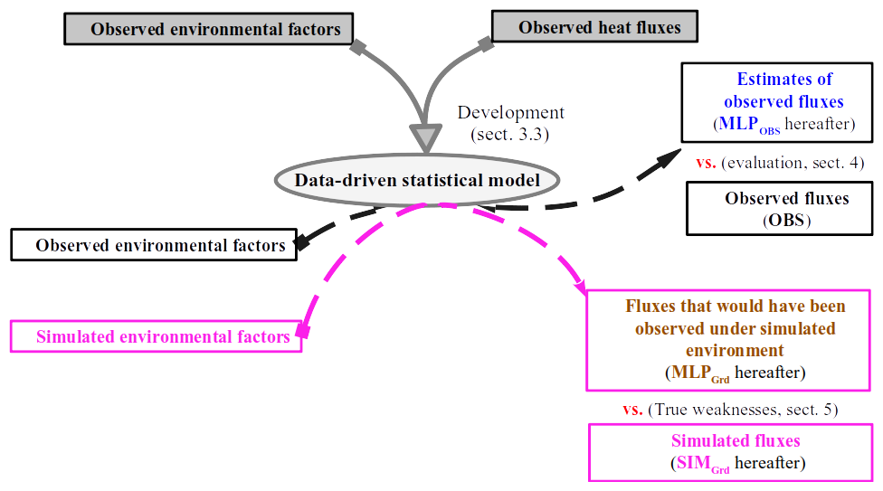
Figure 1 Schematic illustration of our proposed evaluation method. Several years of comprehensive observational data are first utilized to build a data-driven model that statically estimates observed turbulent fluxes (H and LE) along with environmental factors (MLP_OBS). This data-driven model is then applied to approximate the fluxes that could potentially be observed in the simulated weather conditions (MLP_Grd). Thus, comparing the simulated fluxes (SIM_Grd) with MLP_Grd enables a relevant identification of weaknesses in their numerical formulations.

3 Experimental setup

3.1 Observational data

This pilot study is based on high-temporal-resolution data gathered over several years at the Météopole (43.57° N, 1.374° E; 157 $\mathrm{m}\mathrm{a}.\mathrm{s}.\mathrm{l}.$; Etienne, 2022), a measurement site hosted by the Centre National de Recherches Météorologiques (CNRM) in Toulouse, France. This site, operated by Météo-France, is part of the Aerosol, Clouds and Trace Gases Research Infrastructure in France (ACTRIS-FR). The observation facility consists of several colocated ground-based instruments installed in a large grass field. Starting from 24 November 2012, the surface energy budget and the corresponding environmental forcing (soil and overlying meteorological conditions) are continuously documented through a comprehensive set of measurements; the most relevant for our study are listed in Table 1. In addition to turbulent fluxes H and LE, these include the four components of the radiative budget, ground heat flux (G), air temperature (T), relative humidity (RH) at two conventional heights 2 and 10 $\mathrm{m}\mathrm{a}.\mathrm{g}.\mathrm{l}.$ (above ground level), surface pressure (SP) and rainfall (RR), and soil volumetric water content (SWC). The surface and soil temperature are also measured at the Météopole station, but there is a lack of data before 12 July 2015. We thus decided not to use these measurements to avoid limiting the number of samples, which is crucial when building a data-driven statistical model. Sensitivity analysis indicates no significant loss of key information concerning the variability in H and LE.

Table 1 Observational data from the Météopole station used in this study. A negative height corresponds to a soil depth.

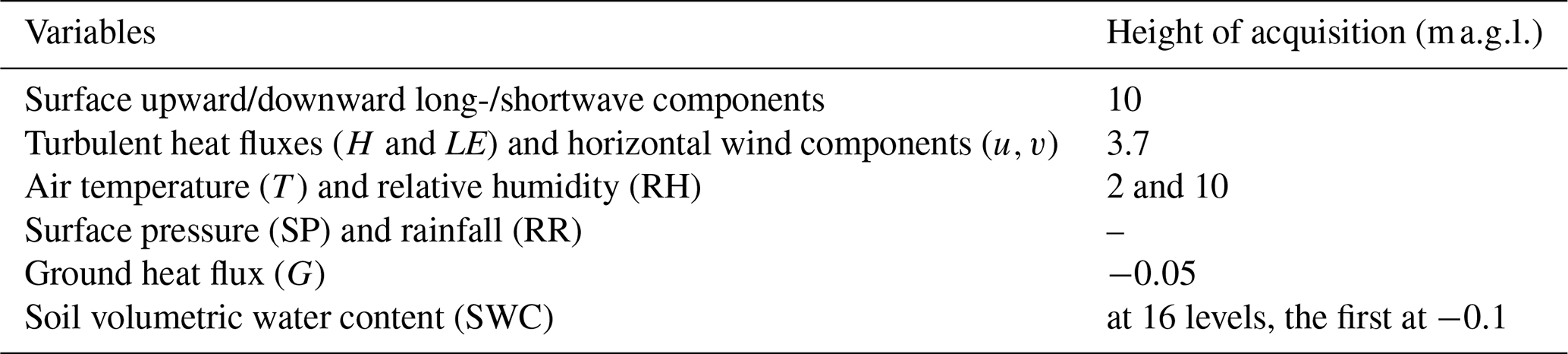
The fluxes H and LE are measured with the EC method (Aubinet et al., 2012) by high-frequency measurements (20 Hz) of three-dimensional components of the wind, T, and water vapor specific humidity (q) with a sonic anemometer and a rapid hygrometer mounted at 3.7 $\mathrm{m}\mathrm{a}.\mathrm{g}.\mathrm{l}$. Eventually, EddyPro 7 software (https://www.licor.com/env/support/EddyPro/software.html, last access: 10 April 2025) is utilized to compute turbulent heat fluxes at a half-hour temporal resolution. Each of these observed fluxes is accompanied by a quality flag by Mauder and Foken (2004) that ranks the measurement into three categories: 0 for high quality, 1 for suitable to be used for research, and 2 for should not be used. Moreover, the rapid hygrometer's accuracy (LI-COR 7500 open path) is highly degraded in wet conditions (fog or rain event). Therefore, the turbulent fluxes are normally not estimated under these conditions, based on the sensor detection of rainfall occurrence. However, wrong measurements could still be performed, as an accumulation of liquid water persists on the sensor.

The environmental parameters are originally acquired every minute and finally archived as half-hourly averages, matching the temporal resolution of turbulent fluxes. Jomé et al. (2023) analyzed the contribution of the surrounding land cover types to the turbulent heat fluxes measured at the Météopole station. It was found that the contribution of grass cover ranges between 80 % and 90 %, with the remaining contribution coming mostly from urbanized areas. The observational data from the Météopole station are freely available via the AERIS platform (https://www.aeris-data.fr/, last access: 10 April 2025). This database undergoes several quality controls and is regularly updated after an annual exercise.

This study is based on the data collected until 23:30 UTC on 31 December 2022, which represent nearly 10 consecutive years of monitoring. The corresponding database contains 117 782 half hours for which the required measurements (Table 1) are simultaneously available, i.e., almost 66.5 % of the samples expected since 00:00 UTC on 24 November 2012. The lack of data is mainly due to the absence of observed turbulent fluxes, mostly under wet conditions. Since the quality and amount of the data on which the data-driven statistical model is built determine its performance, several considerations were applied to select the samples with the most reliable measurements. Firstly, only H and LE with a quality flag of 0 or 1 (Mauder and Foken, 2004) were selected. Due to the strong evolution of continental turbulent heat fluxes throughout the day, several authors have preferred to evaluate numerical simulations under well-established diurnal cycles (e.g., Román-Cascón et al., 2021). For the final selection, we then considered sampling on a daily scale. The half-hourly data included in our analyses are collected during the diurnal cycles (starting at 00:00 UTC) that fulfill the following three conditions: (i) they are described by at least half of the expected samples (i.e., $\mathrm{24}/\mathrm{48}$ of pre-selected samples); (ii) the daily cumulative rainfall is less than 5 mm; and (iii) all the items of Pearson's correlation coefficient matrix between H,LE, and SW^↓ are greater than 0.6. The last two criteria are a compromise to preserve a reasonable number of samples while reducing the amount of data possibly impacted by wet conditions. This leaves us with 80 683 half-hourly samples (around 69 % of all available samples), documenting 2274 diurnal cycles. Figure 2a shows the distribution of these samples per year, and Fig. 2b presents the distribution of the corresponding diurnal cycles per month. None of these diurnal cycles was fully sampled; the rate of data availability is around 74 % on average. The annual cycles from 2015 to 2021 are relatively well sampled. The selected diurnal cycles are homogeneously distributed throughout each year, meaning that the four typical seasons (winter, spring, summer, and autumn) are represented well. There are no selected samples from June to September 2022 (Fig. 2b) due to missing data of LW^↑.

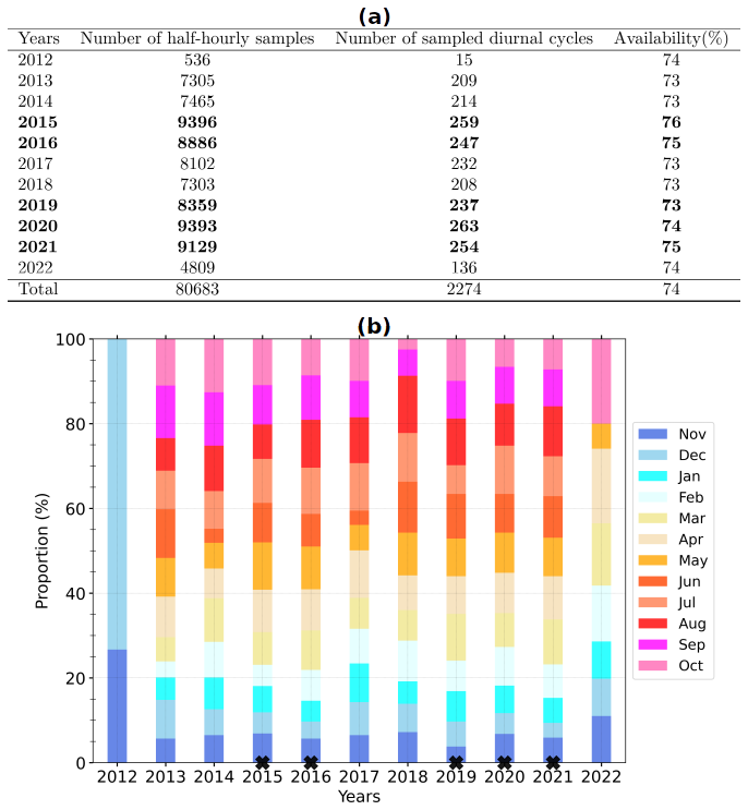
Figure 2 (a) Number of remaining half-hourly samples and diurnal cycles per year after the selection over the period from 24 November 2012 at 00:00 UTC to 31 December 2022 at 23:30 UTC (see text for details) and (b) monthly distribution of these diurnal cycles. The rate of availability is the ratio of the selected half-hourly samples (second column) over the number of samples which fully describe the corresponding diurnal cycles (48 samples, third column). The data of the 5 most covered years (in bold, a, with a black cross at the bottom, b) composed the learning set, and the other years are used as the test set.

3.2 Numerical model data

To test our proposed evaluation method, we used data from an existing climate simulation, carried out with the regional Earth system model of the Institut Pierre-Simon Laplace (RegIPSL). Within the settings of this model, the land surface model ORganising Carbon and Hydrology In Dynamic EcosystEms (ORCHIDEE; Krinner et al., 2005) provides the bottom boundary conditions for the continental surface to the atmospheric model, Weather Research and Forecasting v3.7.1 (WRF; Skamarock et al., 2008). The simulation has been carried out within the framework of the Mediterranean Coordinated Regional Climate Downscaling Experiment (Med-CORDEX) initiative (Ruti et al., 2016) and the European Climate Prediction (EUCP) system H2020 project (Coppola et al., 2020). It covers the Euro-Mediterranean area with a horizontal resolution of 20 km on a Lambert-conformal projection and spans 1 January 1979 to 31 December 2016. The atmospheric vertical column was discretized by 46 hybrid sigma–pressure levels (full eta levels), with 16 levels roughly in the first 2 $\mathrm{km}\mathrm{a}.\mathrm{g}.\mathrm{l}$. The soil column, which extends to 2 m below the ground, was subdivided by 11 nodes, with 7 nodes located within the first 15 cm. For more details, the reader can refer to the studies of Guion et al. (2022), who used this climate simulation to assess the impact of droughts and heat waves on vegetation and wildfires in the western Mediterranean, and Shahi et al. (2022), who used the RegIPSL model to analyze the added value of a convective-permitting climate simulation over the Iberian Peninsula.

The landscape in ORCHIDEE was categorized into 13 main classes, including bare soil and 12 plant functional types (PFTs: eight for forests, two for grasslands, and two for croplands). The total proportion of the grid cell occupied by each class remained constant throughout the simulation. Nonetheless, for PFTs, the proportion effectively occupied by vegetation was allowed to vary, and the non-occupied fraction was defined as bare soil (Ducharne et al., 2018; Alléon, 2022). The bare soil fraction is assumed to contain the urbanized areas. For simulating the surface processes, ORCHIDEE requires several environmental parameters, including surface precipitation and downward SW and LW, as well as air temperature, humidity, and wind just above the ground. These were taken at the lowest vertical level of WRF, located within 20 $\mathrm{m}\mathrm{a}.\mathrm{g}.\mathrm{l}$. The near-surface turbulent heat fluxes are computed using bulk aerodynamic formulations (Ducoudré et al., 1993; Krinner et al., 2005; Alléon, 2022) in an implicit surface–atmosphere coupling (Polcher et al., 1998). Several other useful parameters are also computed, such as surface temperature (T_S), surface albedo, and emissivity, which are needed to calculate the upwelling components of the radiative budget. The calculations are performed at the grid cell scale, by aggregating its landscape into three soil tiles: one for the forest, one for grass and crops, and one for the bare soil. The aerodynamic parameters of the grid cell correspond to the averaged parameters weighted by the effective areal fraction of each soil tile.

The raw output data of this climate simulation have been post-processed, and a variety of specific variables describing atmospheric and land surface conditions have been archived for further use. These include atmospheric variables on half-eta levels (M) such as q, potential temperature (θ), and horizontal wind components (u and v). The surface data involve skin temperature T_S,SP, precipitation rate, H and LE, the four components of the radiative budget, and the underground liquid water content. The most conventional meteorological variables, such as T and RH at 2 $\mathrm{m}\mathrm{a}.\mathrm{g}.\mathrm{l}.$, are also available. The data were stored at a 3 h temporal resolution for all variables except for the underground liquid water content. Specifically, the turbulent heat and radiative fluxes are 3 h time-centered averages, labeled at 01:30, 04:30, 07:30, 10:30, 13:30, 16:30, 19:30, and 22:30 UTC. Meanwhile, atmospheric variables at half-eta levels, q_M,u_M, and v_M, as well as those near the surface, $T_{\mathrm{S}},\text{SP},T_{\mathrm{2}\mathrm{m}}$, and RH_2 m, are nearly instantaneous at 00:00, 03:00, 06:00, 09:00, 12:00, 15:00, 18:00, and 21:00 UTC. The underground water content is archived daily and consists of the height of liquid water within various sublayers, each containing one node.

It would be very interesting to extract the simulation data at a grid cell with a landscape composition that resembles the landscape contribution to the turbulent heat fluxes measured at the Météopole station, as found by Jomé et al. (2023). This grid cell should also be geographically close to the station to preserve the local behavior of atmospheric forcing. However, for all the grid cells located within a distance of 60 km to the station coordinates (e.g., 3 times the simulation horizontal resolution), at least 50 % of the surface is covered by crops and forest PFTs. The areal fraction of grass PFTs ranges from 10 %–21 %. The simulation data are then extracted at the two nearest grid cells to the Météopole site, as is usually done. Figure 3 shows their landscape composition. The proportion of bare soil and crops is respectively greater and smaller in the closest grid cell (Grd1, Fig. 3b). Only the simulation covering the period from 1 January 2012 (the first year of heat flux measurements at the Météopole station) to 31 December 2016 is considered. This period coincides with the selected observation period from 24 November 2012. For consistency with radiative and heat fluxes, the time-centered averages of $q_M,{\mathit{\theta }}_M,u_M,v_M,T_{\mathrm{S}},\text{SP},T_{\mathrm{2}\mathrm{m}}$, and RH_2 m are used. SWC at the soil nodes is calculated as the ratio of liquid water height to the thickness of the corresponding sublayer. For each node, the value of SWC at a given day is assigned to every 3 h timestamp of that day. Similar to the selected observational data, the days with cumulative rainfall exceeding 5 mm were excluded, reducing the simulation data by around 15 %.

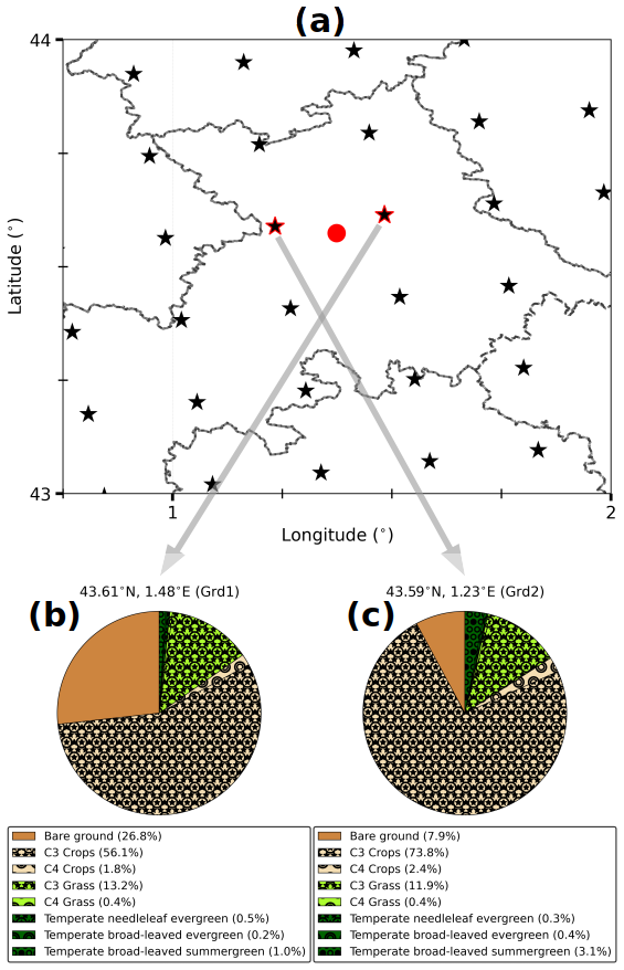
Figure 3 (a) The RegIPSL grid mesh (black stars) around the geographical location of the Météopole site (red circle). The dashed lines indicate the administrative subdivisions. The two nearest grid cells (Grd1 and Grd2) are highlighted with red edges. (b, c) Landscape composition in these two grid cells, with Grd1 (b) being the closest.

3.3 The data-driven statistical model

Since the fluxes H and LE are continuous variables, our problem is formulated as multivariate regression settings. There are several ways to perform regression with ANNs. The easiest is to exploit the most basic ANN, the feed-forward network, also known as the multi-layer perceptron (MLP). Due to its exceptional ability to approximate complex multivariate functions, MLP has become the most widely used type of ANN. Accordingly, our data-driven statistical model is built using MLP. This section begins by briefly introducing this type of ANN. Subsequently, the implementation of the statistical model with half-hourly observational data is detailed. Finally, the challenges involved in its application to the data from climate simulations are outlined.

3.3.1 The multi-layer perceptron

The elementary unit of ANNs is the mathematical neuron (Rosenblatt, 1960), which is illustrated in Fig. 4. It is a numerical computational unit that receives information through synaptic connections characterized by weights (w) and provides a response using an activation function (f) and a bias (b), as follows:

$$\begin{array}{}\text{(3)}& {\displaystyle }{\displaystyle }o=f\left(b+\sum _{j=\mathrm{1}}^N{w}_j\cdot x_j\right),\end{array}$$

where N is the number of input variables. In general, the input data of f and its output range within $[-\mathrm{1},\mathrm{1}]$. The neuron's behavior, either linear or non-linear, is defined by its activation function. Although there are many types of activation functions, sigmoid-like functions (e.g., logistic and hyperbolic tangent) and the identity function are commonly used for regression (Zhang, 2008).

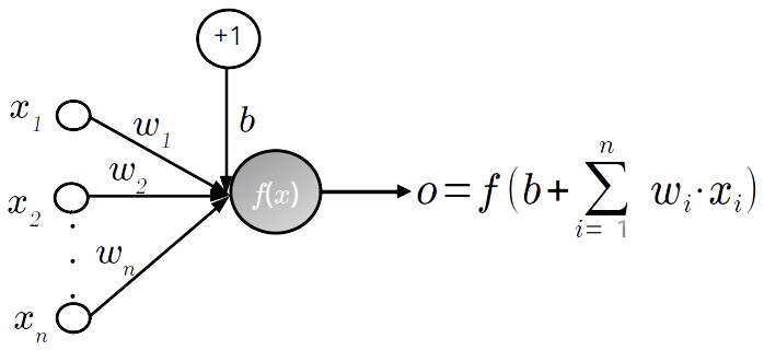
Figure 4 Schematic illustration of a mathematical neuron (adapted from Zhang, 2008): x_i and w_i correspond to its numerical inputs and synaptic weights respectively, whereas o is the response based on its activation function (f) and bias (b). This latter is schematized by an input variable with a value and weight equal to +1 and b respectively.

The MLP is a supervised ANN, which consists of fully interconnected neurons organized in successive layers (see Fig. 5 for illustration). These layers include an input layer to receive the predictors, an output layer to get the outcome, and at least one intermediate layer between them – the so-called hidden layer(s). There is one neuron per input and output variable. The neurons in the input layer just carry the data without any calculations. The hidden layer(s) form the computational core of MLP. Although the topography of hidden layers (number of layers and neurons) has an impact on the network's capability to approximate the relationships, there is not yet a universal rule defining the most suited topography for a given problem. Thus, finding an appropriate configuration for hidden layers (number of layers and neurons) is generally a non-trivial and uphill task with expensive computational costs.

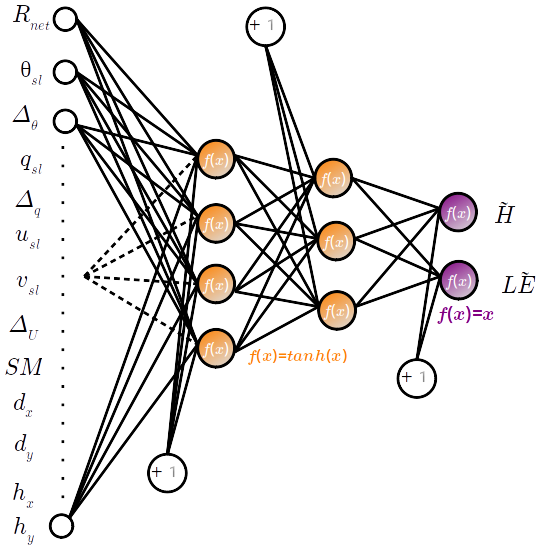
Figure 5 Architecture of the MLP used in this study. The input variables are described in Table 2.

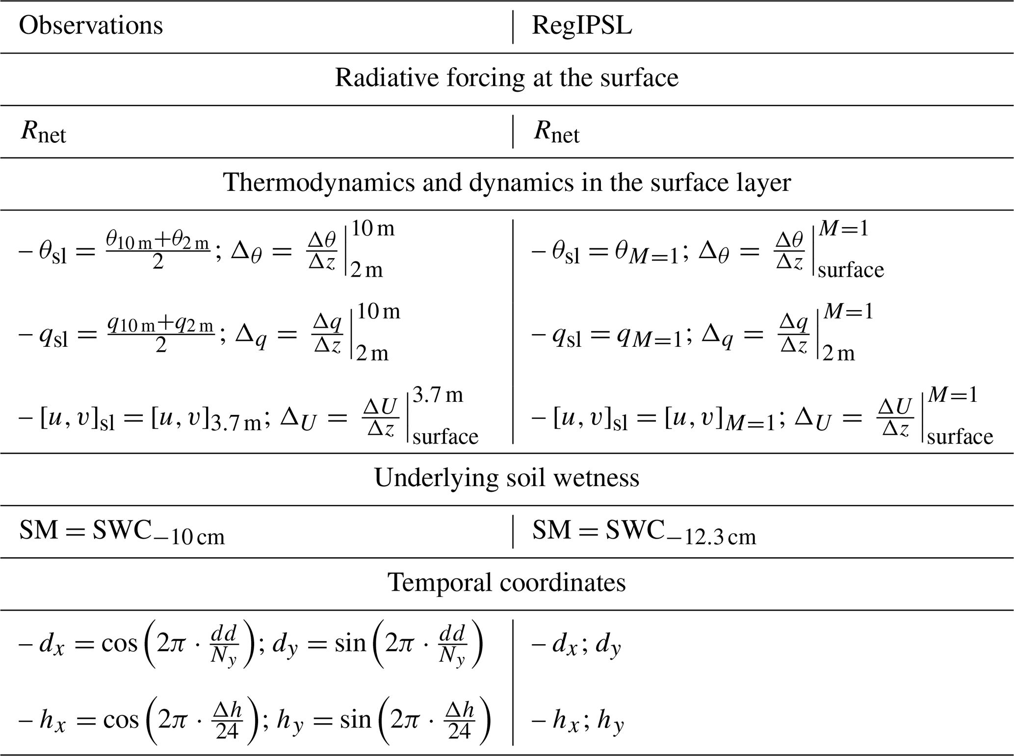
Table 2 The 13 MLP input variables, derived from observational data and their equivalent extracted from RegIPSL data. dd,Δh, and N_y included in the expressions of the temporal coordinates are the Julian date, hours relative to sunrise on dd, and number of days in the year respectively.

As a supervised ANN, MLP acquires knowledge about its task through a learning stage. During this stage, the network is provided with examples of paired predictors and desired outputs, and its weights and biases adjust accordingly. The MLP's understanding of physics laws then entirely relies upon the quality and amount of data on which it has learned. Thus, the more consistent the examples, the greater the chances of the MLP being accurate over unseen input data. The learning data are usually separated into two disjoint subsets: training and validation. The MLP weights and biases are updated using a backpropagation optimization technique, which minimizes an error metric calculated on the training data between the MLP outputs and the desired values. The mean square error (MSE) is the common error metric (Zhang, 2008) for regression. In general, there are three modes in which backpropagation optimization may be applied: (i) the “online” mode, in which the network weights and biases are updated for each example in the training set; (ii) the “batch” mode, in which all the training data are considered at once; and (iii) the “mini-batch” mode, which is a mixture of the first two and achieves their advantages while limiting their inconveniences. The training data are subdivided into a smaller fixed number of samples (the mini-batch), which are used for modifying weights and biases. The default mini-batch size is 32. Another key parameter of the learning stage is the number of training data passages through the network, also called epochs (Chicco, 2017; Zhang, 2008; Kruse et al., 2013). Indeed, with small epochs, the network would not understand the complexity of the data, leading to an underfitting. By contrast, large epochs may lead to overfitting; the network would capture all the details of the training data while performing badly on unknown data. The validation data serve to assess the network performance during the updating of its weights and biases. Thus, a fairly large number of epochs can be considered to prevent underfitting, while early stopping is applied when performance on the validation set no longer improves, thereby avoiding overfitting.

Thus, the implementation of MLP can be split into three main points:

• i.

  Define a set of relevant predictors based on the variables to be approximated.

• ii.

  Select learning data such that they would contain sufficient examples to statistically describe the relationships between predictors and targeted variables.

• iii.

  Find a suitable MLP setting (topology of hidden layer(s), activation function, etc.) through sensitivity experimentation.

Before processing with MLP, data should be scaled (i) for consistency with f and (ii) to circumvent the relevance of variables due to their magnitude. Moreover, the backpropagation algorithm is stochastic, which often leads to variability in the final weights and biases of MLP each time the network is retrained with the same data. Indeed, the final state may correspond to a local minimum of the error metric (Zhang, 2008). Although the difference between the MLP outputs is usually slight, it can be annoying not to get the same results. The ensemble learning approach (Ganaie et al., 2022) may limit the instability of the MLP-based estimates and get closer to the optimal estimate. Instead of training a single MLP, this approach involves training multiple MLPs and then averaging their outputs for regression problems. One of the standard strategies for generating these MLPs is bagging (Breiman, 1996; Khwaja et al., 2015); a base MLP is trained on a redistributed version of the original training or learning set.

3.3.2 Implementation

In this work, each MLP is implemented using TensorFlow-Keras (version 2, Abadi et al., 2016), a Python library specifically designed for ANNs, known for its user-friendly interface. Unless otherwise mentioned, the default parameters are used. The three points mentioned above are addressed as follows:

• i.

  As MLP predictors, we use 13 variables that can be derived from observational and simulation data while still having the same physical meaning. Their formulations are shown in Table 2. Indeed, H and LE are theoretically quasi-constant within the surface layer and strongly related to near-surface radiative, thermodynamic, and dynamical forcing. Moreover, their relative predominance is controlled by the wetness of the uppermost part of the soil. In numerical simulations, the atmospheric level just above the ground is usually the top of the surface layer. Therefore, considering the observed variables in Table 1 and the variables from the simulation that have been archived, we derived a set of nine physical variables that may analogously summarize the environmental forcing in the surface layer. They include the radiative-energy-governing surface processes (R_net), the meteorological conditions in the surface layer (${\mathit{\theta }}_{\text{sl}},{\mathrm{\Delta }}_{\mathit{\theta }},q_{\text{sl}},{\mathrm{\Delta }}_q,u_{\text{sl}},v_{\text{sl}},{\mathrm{\Delta }}_U$), and the moisture in the uppermost soil layer (SM). Eventually, four trigonometric temporal coordinates are added to describe seasonal (d_x,d_y) and diurnal (h_x,h_y) cycles. Under the observed environment, SM is defined by SWC_−10 cm (the first depth of soil moisture measurements), and the meteorological variables are calculated assuming that the surface layer always extends above 10 $\mathrm{m}\mathrm{a}.\mathrm{g}.\mathrm{l}.$ For the simulated environment, SM then corresponds to SWC_−12.3 cm (the nearest node to the measurement depth). Diagnostic variables derived from numerical simulation (T_2 m,RH_2 m) are susceptible to containing bias due to the interpolation technique and the inconsistency of terrain elevation. To avoid these uncertainties, the meteorological variables are taken directly at the first half-eta level (M=1, around 8 $\mathrm{m}\mathrm{a}.\mathrm{g}.\mathrm{l}.$) as much as possible. In both observed and simulated environments, Δ_U is calculated assuming a null horizontal wind speed at the ground. Due to missing data, the sunrise hour required to compute h_x and h_y was retrieved using the astral package (version 3.0) and rounded to the nearest half hour.

• ii.

  To train the statistical model over as many multivariate cases as possible, the half-hour observational data from the 5 most covered years (Fig. 2) were gathered as the learning set. The remaining data were reserved for assessing the model's ability to generalize, referred to as the test set.

• iii.

  Since H and LE are complementary fluxes and to avoid excessive sensitivity experiments in search of a relevant architecture for MLP, the neurons in the output layer were set to two, one for each flux. Following the literature (Kumar et al., 2011; Leufen and Schädler, 2019; Kelley and Pardyjak, 2019; Kelley et al., 2020), hyperbolic tangent and identical functions were used as the activation functions for neurons of the hidden and output layers respectively. The weight and bias optimization was carried out with the Adam AMSGrad backpropagation algorithm (Kingma and Ba, 2017; Reddi et al., 2019) in a default mini-batch mode, and MSE was chosen as the error to minimize. Based on preliminary results, we opted for the same strategy of network training used by Leufen and Schädler (2019). The network update stops at most after 1000 epochs. Otherwise, the update is stopped early if the MSE on the validation data does not improve after 50 successive epochs, and then the network state is finally set to the epoch with the best MSE.

The input and output data are scaled to the interval [0,1], similarly to Leufen and Schädler (2019), as follows:

$$\begin{array}{}\text{(4)}& {\displaystyle }{\displaystyle }\stackrel{\mathrm{̃}}{x}={\displaystyle \frac{x-x_{\text{min}}}{x_{\text{max}}-x_{\text{min}}}},\end{array}$$

where x_min and x_max correspond to the extreme values. They are set to the theoretical values of the trigonometric functions (e.g., −1 and 1 respectively) for the four temporal coordinates. For the other nine physical parameters, these values are set so that the resulting interval strictly holds both the observational and the RegIPSL data (see Fig. A1 in the Appendix).

The MLP base architecture used in this study involves two hidden layers with four and three neurons respectively (Fig. 5). This was found through several series of sensitivity experiments with the learning set (not shown). A bagging-based strategy was used to account for the strong inter-annual variability of H and LE in their statistically based estimates. Indeed, a 5-fold cross-validation (Andersen and Martinez, 1999) with year-wise data splitting was applied to the learning set to generate 55 bagged MLPs. Cyclically, the data from 1 year were used as the validation set, whilst the others composed the training set, and 11 MLPs were trained by randomly initializing weights and biases along with a shuffling of the training data before composing mini-batch subsets. In this way, each example in the learning set was used at least once as validation or training data. Even though the number 11 was arbitrarily chosen based on the available computing resources, it ensures the repeatability of estimates. Thus, the statistically based estimates of observed fluxes are the average across the individual MLP outputs. In the following, we refer to these as MLP-based fluxes or estimates.

3.3.3 Application to data from numerical model

The MLP-based model is built using half-hour observational data to take advantage of more samples. After that, it is applied to the 3 h simulation data to provide H and LE that are likely to be observed in the simulated environment. This assumes that simulated and observed environments share a common space, and the learning data represent that space. On one hand, the difference in temporal resolution could introduce artificial errors that might impact both the statistical model's performance and the comparison results. These potential impacts are discussed at the beginning of Sect. 5. On the other hand, if the simulated environment does not have similar structures (distribution and interval ranges of input variables) to the observations, the statistical model may perform poorly. Indeed, MLP has a good interpolation capability but may not correctly extrapolate beyond the ranges of values it has learned (Bonnasse-Gahot, 2022). Yet, for four of the nine physical variables (${\mathrm{\Delta }}_{\mathit{\theta }},{\mathrm{\Delta }}_q,u_{\text{sl}}$, and v_sl), the simulation data spread beyond the observed values (Fig. A1). A rigorous application of machine learning techniques requires the use of transfer learning to mitigate performance loss when a trained ANN is applied to data originating from another source (Day and Khoshgoftaar, 2017). Since the observed H and LE associated with the simulated environment are unknown, the most challenging transfer learning approach, unsupervised domain adaptation, would normally be used in our case. Numerous methods are available for achieving unsupervised domain adaptation. We tried the easiest and most popular methods over the simulation input data, such as correlation alignment (Sun et al., 2016), feature augmentation (Daumé III, 2009), subspace alignment (Fernando et al., 2013), transfer component analysis (Pan et al., 2011), and feature selection (Uguroglu and Carbonell, 2011) as implemented in the ADAPT library (version 0.4.2, de Mathelin et al., 2023). We either get unreasonable fluxes, particularly in stable conditions, or have fluxes that vary from one method to another, so it is hard to conclude the most suitable method. The most sophisticated methods require the use of an encoder, which may be an ANN, with the laborious and time-consuming task of finding its appropriate configuration. Further investigations are then needed to find a suited unsupervised domain adaptation method, but that is beyond the scope of this paper.

At this stage, our proposed evaluation method does not yet include any transfer learning method. Under the traditional assumption that training and testing data come from the same distribution and input space (Aggarwal, 2014), the MLP-based statistical model is directly applied to simulation data. Nonetheless, to gain insight into performance loss, the relative contribution of each predictor to flux estimates is calculated using the SHapley Additive exPlanations (SHAP) algorithm (Lundberg and Lee, 2017). SHAP is attractive because it unifies several common methods for interpreting the approximation with ANN. It is based on the game theory approach; for an individual game (MLP outputs), contributions (called SHAP values) are assigned to each player (predictor). The average of the SHAP absolute value in several instances is then used to measure the predictor influence. The higher the corresponding SHAP value, the more the input variable contributes on average.

4 Assessing the data-driven statistical model

As mentioned previously, the MLP-based H and LE are the average over the outputs of 55 MLPs trained with the learning set. The key objective in machine learning is generalization, which means that the data-driven model should perform well under known and unknown conditions. This section discusses the performance of our statistical model on learning and test sets.

Figure 6 compares half-hourly MLP-based fluxes (MLP_OBS) against their observed values (OBS), for learning and test sets (left and right panels respectively). It shows H and LE (top and middle panels respectively) and the total turbulent heat flux H+LE (bottom panels). Overall, the root mean square errors (RMSEs) range from 20–30 W m⁻², and Pearson's correlation coefficients (r) are greater than 0.95, indicating excellent agreement between estimated and observed fluxes. Interestingly, H+LE is particularly well approximated, despite not being a direct output of MLPs. Furthermore, the RMSE increases by less than 20 %, and the correlation is almost the same from learning to test data. Hence, under both known and unknown observed conditions, the statistical model performs similarly on average, demonstrating a fairly good generalization ability. Besides this good performance, some noticeable shortcomings appear in both the learning and the test sets. On the one hand, MLP_OBS H is bound to about −50 W m⁻², while values below −100 W m⁻² are observed (Fig. 6a and b). On the other hand, MLP_OBS LE tends to underestimate observed LE above 200 W m⁻² (Fig. 6c and d), especially for the test set. This indicates that the statistical model struggles to estimate large LE and negative H, which are associated with highly unstable and stable surface layer regimes respectively.

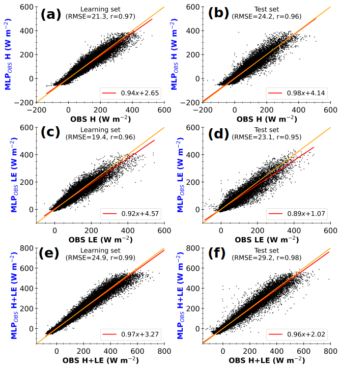
Figure 6 Half-hourly MLP-based estimates of observed sensible heat flux (MLP_OBS H, a, b), latent heat flux (MLP_OBS LE, c, d), and total turbulent heat flux (MLP_OBS H+LE, e, f) with observed input data against observed fluxes (OBS), for learning (a, c, e) and test (b, d, f) sets. The values at the top of each panel correspond to root mean square error (RMSE) and Pearson's correlation coefficient. The lines in red and orange represent the linear regression and identical fits respectively. The axis labels are colored according to the schematic illustration in Fig. 1 (right side).

Figure 7 shows the cumulative distribution functions (CDFs) of RES (Eq. 2) calculated with half-hourly observed R_net−G together with OBS and MLP_OBS fluxes. For both learning and test sets (Fig. 7a and b resp.), CDFs of OBS and MLP_OBS are close, but the MLP underestimates the strong (negative or positive) RES values. Although the sample size is different for these two sets, their CDF curves look quite similar, implying that they are individually representative of the main local characteristics of energy imbalance. Closer inspection showed that the statistical model provides smoothed fluxes that preserve the striking relationship between OBS H+LE and R_net−G (not shown). This smoothing is the main cause of intermittent departures between the CDF curves. Overall, the CDFs are smaller than 0.15 for RES lower than 20 %, indicating that both OBS H+LE and MLP_OBS H+LE are smaller than R_net−G in the majority of cases. This tendency is systematic for large H+LE (not shown). Thus, the statistical model carries the limitations of observed turbulent heat fluxes. The representativeness of turbulent heat fluxes measured at the permanent Météopole site on the coarser horizontal scale of numerical models is being examined as part of the MOSAI project (e.g., Jomé et al., 2023).

Figure 7 Cumulative density functions (CDFs) of RES (Eq. 2) calculated with half-hourly observed turbulent heat fluxes (OBS, in black) and competing MLP-based estimates (MLP_OBS, in blue) for the learning set (a) and test set (b) in Fig. 6.

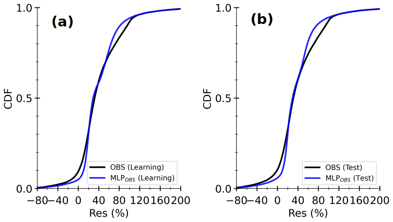
Figure 8 shows the composite seasonal cycles of OBS and MLP_OBS fluxes for the learning and test sets (left and right panels respectively). The observed H+LE presents similar seasonal cycles for both sets, with a peak from April to September (Fig. 8c and f). However, observed H and LE do not typically present the same seasonal cycle. Indeed, from April to September, H(LE) is on average stronger (weaker) in the learning set than in the test set. In the learning set, LE predominates over H from March to June, with the reverse occurring from July to October (Fig. 8a and b), whereas in the test set, the predominance of H starts later in August, since LE slowly decreases from May to July (Fig. 8d and e). The inter-annual variability presented in Fig. A2 explains this disparity. Indeed, the year 2018 presents a seasonal cycle of H and LE that differs from the one of other years, which different vegetation dynamics, driven by different atmospheric conditions, may explain. This highlights the importance of covering several annual cycles to effectively train the MLPs.

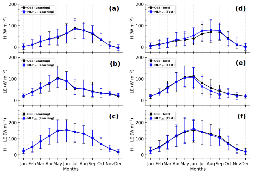
Figure 8 Composite monthly averages of observed (OBS in black) and MLP-based (MLP_OBS in blue) sensible heat flux (H, a, d), latent heat flux (LE, b, e), and total turbulent heat flux (H+LE, c, f) for the learning (a–c) and test sets (d–f) respectively. The solid lines represent the means, and the error bars correspond to the 10th and 90th percentiles, calculated by gathering the daily averages of half-hourly samples in Fig. 6.

Overall, the MLP_OBS fluxes correctly reproduce the observed seasonal cycles along with day-to-day variability for both learning and test sets. This is particularly true for the total turbulent heat flux (Fig. 8c and f). Interestingly, the relative predominance between H and LE is remarkably well replicated in the two sets. In the learning set, the absolute difference between estimated and observed fluxes remains smaller than 5 W m⁻² for all the fluxes. However, in the test set, striking differences appear between May and September, when the total turbulent heat flux is at its maximum. Indeed, while MLP_OBS H+LE is quite similar to observations (Fig. 8f), MLP_OBS H overestimates observations (Fig. 8d) by more than 10 W m⁻² in June and July, and MLP_OBS LE underestimates observations by more than 14 W m⁻² from July to September (Fig. 8e). This likely comes from the fact that the MLPs have learned respectively weaker LE and stronger H on average (Figs. 8 and A2).

In conclusion, the statistical model, constructed with half-hourly observational data, provides highly consistent estimates of observed H and LE. It especially approximates the total flux H+LE quite well. The non-closure of SEB embedded in the observed fluxes is also reproduced but slightly reduced for the strongest values. Its performance in terms of RMSE and linear correlation ranges within the best reported by the literature on surface parameterization schemes (e.g., Liu et al., 2013; Leufen and Schädler, 2019; Román-Cascón et al., 2021). In particular, the relative predominance between heating and evaporation is faithfully reproduced at the seasonal scale. The most fundamental local links between turbulent fluxes and environmental factors seem to be well captured by the data-driven model. However, it shows limitations with estimating large LE and negative H and does not generalize well in the spring and summer months. The limited number of samples in the learning set and/or the MLP input variables do likely not fully convey the strong inter-annual variability of turbulent heat fluxes.

Increasing the learning data at the expense of the test data does not noticeably improve the generalization ability of the statistical model (not shown). Moreover, uncertainties will always remain when the statistical model is applied to unseen data and cannot be assessed in the absence of corresponding observations, as is the case for numerical simulations. By convention, 30 years of observational data is required for good climatological coverage, while around 10 years is currently available at the Météopole permanent site. The spring and summer seasons are usually characterized by intense vegetation activity. Moreover, the relationship between surface latent heat flux and soil moisture could be modulated by the state of the vegetation (e.g., Román-Cascón et al., 2020). However, the MLP input variables lack a key factor that could capture vegetation dynamics, such as the leaf area index (LAI). Adding such a parameter to the input variables would provide a more robust description of the annual variability of surface turbulent heat fluxes. This is likely to enhance the generalization ability of the statistical model, especially during the spring and summer seasons.

5 Using the data-driven statistical model to evaluate simulated surface turbulent heat fluxes

The simulated surface turbulent heat fluxes from 1 January 2012 to 31 December 2016, by the RegIPSL model, are evaluated in this section. The benefits of our proposed evaluation approach, compared to the traditional direct comparison between observed and simulated time series, are discussed.

For as much consistency as possible with the archived simulation data, 3 h of “adapted” observational data (${\text{OBS}}^{\prime },\mathrm{15}\mathrm{739}$ samples in total from November 2012 to December 2022) was derived from half-hour observations (see Table 1). Indeed, $\text{SWC},H,\mathit{\text{LE}}$, and the four radiative fluxes were time-centered averaged on a 3 h window to get the same timestamps. The timestamp is excluded when more than half of the expected half-hour data (e.g., three out of six expected samples) are missing. Half-hour data at these timestamps are used directly when available for the other variables ($T,\text{RH},\text{SP},u$, and v). If not available, T,RH, and SP values are obtained through linear interpolation, while u and v are taken from the nearest half hour. First, the sensitivity of the data-driven model's performance to changes in temporal resolution and the effects of simulated data extending beyond the learning range are assessed. Then, the data-driven model is applied to evaluate the simulated heat fluxes over the common period.

5.1 Impact of temporal resolution and extrapolation on flux estimates using the data-driven model

Table 3 shows the RMSE, r, and linear regression coefficients (slope and intercept) obtained when all MLP_OBS H and LE from November 2012 to December 2022 are compared with their target values, for both the adapted 3 h OBS^′ and the half-hour OBS from which OBS^′ was derived. Figure 9 shows their composite diurnal cycles for the sub-periods during which the fluxes are weaker (November, December, January, and February), stronger with a predominance of LE (March, April, May, and June), and stronger with a predominance of H (July, August, September, and October). The RMSE of ${\text{MLP}}_{{\text{OBS}}^{\prime }}$ improves by 4 W m⁻², and the other parameters in Table 3 remain the same, between OBS and OBS^′ datasets. The composite diurnal cycles of the observed fluxes and the MLP-based estimates for both temporal resolutions align closely with each other. This indicates that the mismatches between half-hour and coarser 3 h time resolutions do not significantly affect the performance of the statistical model.

Table 3 Comparison of the root mean square error, linear correlation, and linear regression fitting coefficients (slope and intercept) when applying the MLP-based statistical model to half-hour raw and 3 h average observational data. The statistical model has been constructed using the half-hour sampling of the learning set (Fig. 2a).

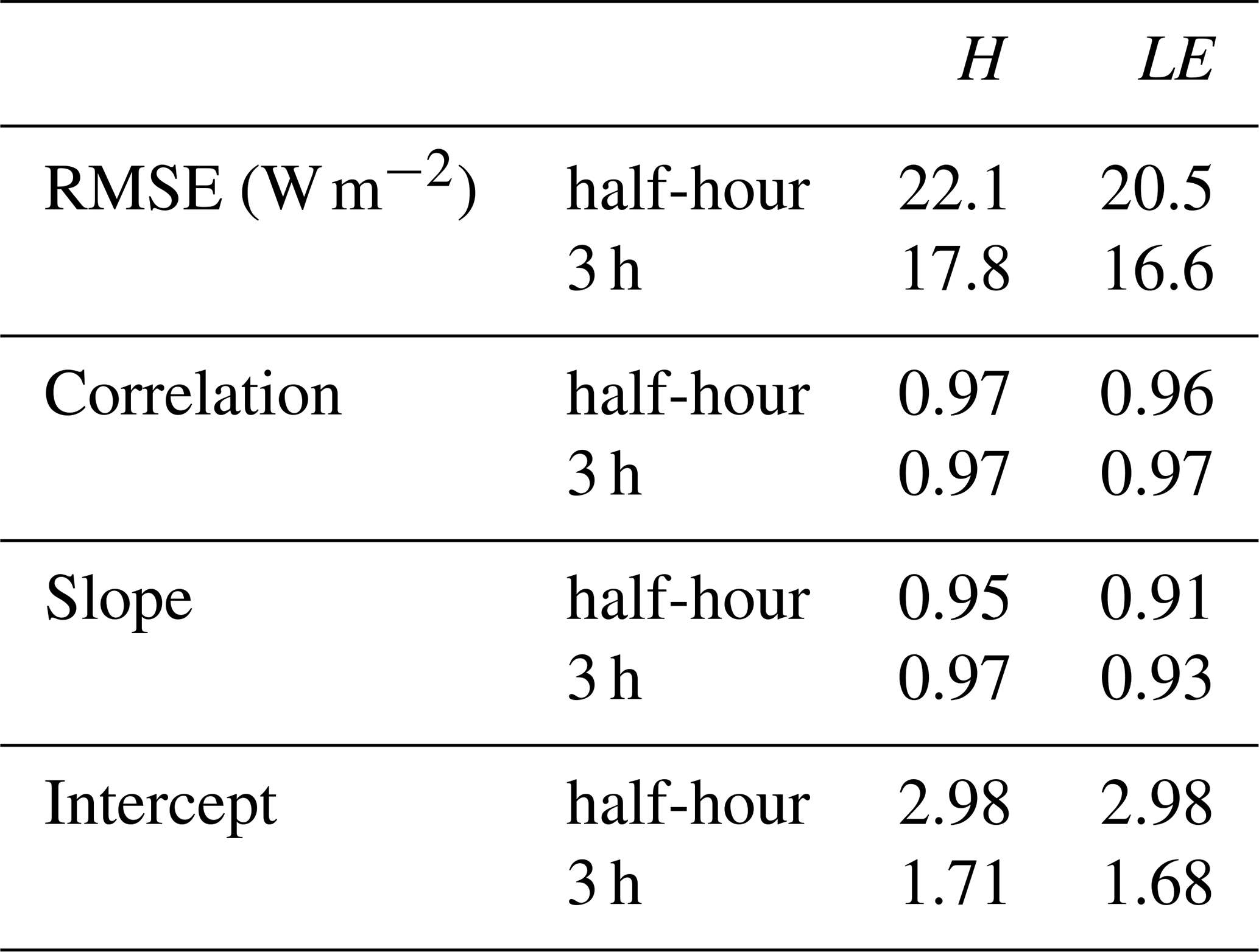
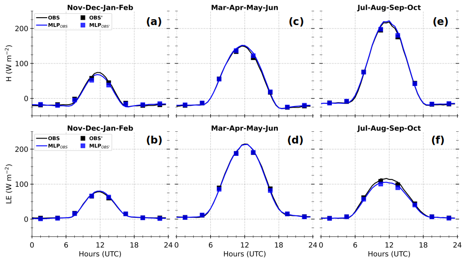
Figure 9 Composite diurnal cycles of half-hour and 3 h observed heat fluxes (OBS and OBS^′, in black) and their competing MLP-based estimates (MLP_OBS and ${\text{MLP}}_{{\text{OBS}}^{\prime }}$ respectively, in blue), for H (a, c, e) and LE (b, d, f), by splitting the annual cycle into three typical sub-periods (see the text for more details). They are calculated based on diurnal cycles where at least six out of eight expected OBS^′ samples are available (approximately 85 % of all selected diurnal cycles).

Figure 10 presents averages of SHAP absolute values for each input variable across the trained MLPs, for the MLP-based H and LE for learning and test sets (in Fig. 6) and simulated environments at Grd1 and Grd2. The variables are ranked on the y axis in descending order according to their values at Grd1, the nearest geographical grid cell. Note that the SHAP value increases with the relative contribution of the input variable. Thus, this figure allows for a discussion of performance loss due to extrapolation, e.g., when the input data extend beyond the learning interval.

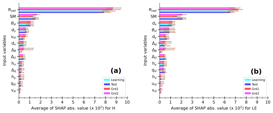
Figure 10 Averages of SHAP absolute values for each input variable in MLP-based estimates of H (a) and LE (b) within the simulated environment at Grd1 and Grd2 and the observed environment of learning and test sets, according to the caption. For a given MLP, the SHAP absolute values are calculated for each estimate and then averaged over the samples of each dataset. The colored bars indicate the median values, and the error bars correspond to the minimum and maximum values across the 55 trained MLPs that compose the statistical model. In each panel, the input variables are ranked in descending order under the simulated environment at Grd1.

Regardless of the environment, R_net is by far the most contributing variable, followed by SM and θ_sl for both H and LE estimates. Thus, the trained MLPs composing the statistical model clearly understood that the net radiative budget at the surface is the primary driver of turbulent heat fluxes and that the soil wetness is a crucial factor for the partitioning between heating and evaporation. This probably explains the better agreement between observed fluxes and the corresponding MLP_OBS at coarser, seasonal, and 3 h timescales, since the noise in the observational data is reduced. The importance of the other variables varies with the environment, the grid cells, and the fluxes. Notably, Δ_θ is one of the least influential variables under observed conditions, unlike in the simulated environment. This demonstrates that the statistical model takes into consideration changing environmental contexts. Overall, the aggregated contribution of the three physical variables (Δ_θ,u_sl, and v_sl), whose simulated values spread beyond the learning interval, is overall smaller than 20 % of the aggregated contribution of R_net, SM, and θ_sl. Therefore, we hypothesize a modest loss of performance due to extrapolation when the statistical model is directly applied to data from the RegIPSL model.

5.2 Evaluating the simulated heat fluxes using the data-driven model

Remember that MLP-based fluxes are approximations of observed fluxes in a given environmental forcing (see Sect. 4). When applied to the simulation, they correspond to the fluxes that would have been measured if the simulated conditions were effectively observed. In the following, OBS^′ data (e.g., 3 h time-centered averages) are used as observed conditions. They are referred to as OBS for simplicity.

The scatter plots in Fig. 11 illustrate the consistency of the MLP-based fluxes in the simulated environment. They also highlight errors resulting from disparities in observed and simulated environmental forcing. The scatter plots compare 3 h MLP-based fluxes with environmental conditions at Grd1 (MLP_Grd1) against the corresponding 3 h fluxes (OBS, left panels) and MLP-based fluxes in observed conditions (MLP_OBS, right panels). The figure only includes the timestamps between 24 November 2012 and 31 December 2016, for which both simulated and corresponding OBS are available, accounting for around 50 % of all simulation data. In each panel, the flux varies within the same interval range, between −50 and 400 W m⁻² for H and LE and between −50 and 500 W m⁻² for H+LE. Moreover, the correlation coefficient is greater than or equal to 0.9, indicating that the variability in MLP_Grd1 fluxes is consistent with OBS and MLP_OBS. These findings also hold for the second grid cell (Fig. A3). Hence, the disparities between simulated and observed fluxes mostly lie in their magnitudes. Since the difference is much more pronounced for large fluxes, the divergence would occur mainly during daylight hours. MLP_Grd1 H and H+LE are stronger than those observed. The same tendency has been found when comparing simulated R_net to observations (not shown).

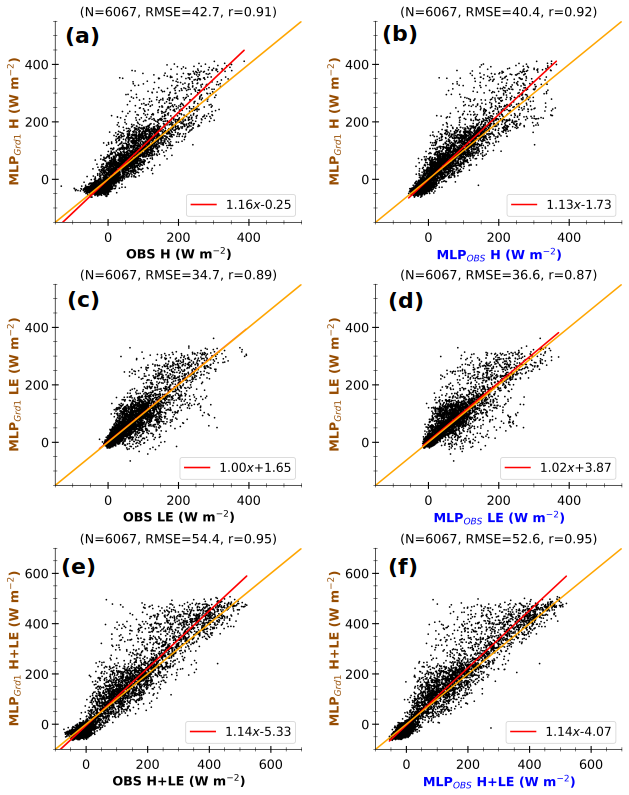
Figure 11 Comparison of 3 h MLP-based fluxes in the simulated environment at Grd1 (MLP_Grd1) against 3 h observations (OBS, a, c, e) and MLP-based fluxes in the associated environment (MLP_OBS, b, d, f) at the Météopole site, for H (a, b), LE (c, d), and H+LE (e, f). The data include only 3 h timestamps between 24 November 2012 and 31 December 2016, for which both simulation and observational data are available. The values at the top of each panel correspond to the number of samples (N), the root mean square error (RMSE), and Pearson's correlation coefficient (r). The lines in red and orange represent the linear regression and identical fits respectively. The axis labels are colored according to the schematic illustration in Fig. 1.

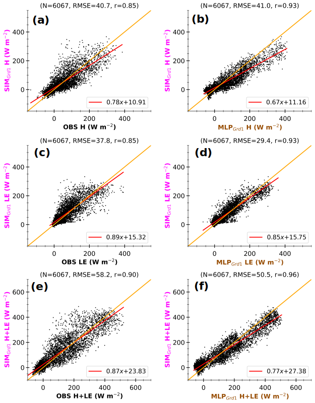
Figure 12 Comparison of 3 h simulated fluxes at Grd1 (SIM_Grd1) with observed fluxes at the Météopole site (OBS, a, c, e) and MLP-based estimates in the simulated environment (MLP_Grd1, b, d, f) for H (a, b), LE (c, d), and H+LE (e, f). The data correspond to the same timestamps as in Fig. 11. The values at the top of each panel correspond to the number of instances (N), the root mean square error (RMSE), and Pearson's correlation coefficient (r). The lines in red and orange represent the linear and ideal fits respectively. The axis labels are colored according to the schematic illustration in Fig. 1.

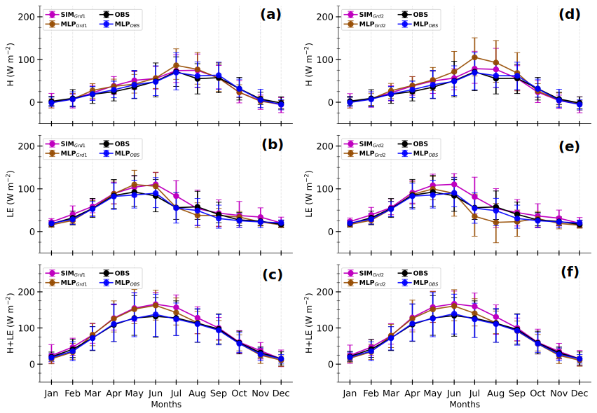
Figure 13 Composite monthly averages of heat fluxes simulated at Grd1 and Grd2 (SIM_Grd1, a–c, and SIM_Grd2, d–f, respectively); MLP-based estimates for their respective environments (MLP_Grd1 and MLP_Grd2) observed at the Météopole site (OBS); and MLP-based estimates in the observed environment (MLP_OBS) for H (a, d), LE (b, e), and H+LE (c, f). The curve colors are according to the schematic illustration in Fig. 1. The solid lines correspond to the means, and the error bars represent the 10th and 90th percentiles, calculated by gathering daily averages using 3 h data. Only the timestamps between 1 December 2012 and 31 December 2016, for which both simulation and observational data are available, have been considered. The days involving fewer than six timestamps were excluded.

Figure 12 compares 3 h simulated heat fluxes at Grd1 (SIM_Grd1) to OBS and MLP_Grd1 (left and right panels respectively) at the same timestamps as in Fig. 11. The scatter is considerably reduced with a better alignment along the linear regression fit when MLP_Grd1 values are used as the reference values instead of OBS. These changes agree well with a reduction in uncertainties, particularly those related to the disparities in environmental conditions. The non-closure of SEB for MLP-based fluxes may (Fig. 7) explain the imperfect fit between SIM_Grd1 H+LE and corresponding MLP_Grd1. This suggests that substantial uncertainties remain. Nonetheless, comparing with MLP_Grd1 better highlights the shortcomings of the surface scheme than a direct comparison with OBS, as the bias in R_net is frozen. According to MLP_Grd1, the surface scheme tends to quasi-systematically underestimate large H (Fig. 12a and b). This tendency is more pronounced for Grd2 (Fig. A4), which comprises a smaller fraction of bare soil and a larger cropland fraction, which enhance evaporation. In contrast, the simulated environment promotes overestimating large observed H (Figs. 11 and A3a and b), mostly due to higher R_net and weaker SM. Thus, by using the statistical model, we can detect that the R_net overestimation compensates for and hides an underestimation of H in RegIPSL. This underestimation may be due to (i) incorrect surface land use (with crop instead of grass and bare soil instead of urban area) and (ii) inadequate formulations of fluxes.

Additionally, SIM_Grd1 and SIM_Grd2 differ very slightly. As a result, the direct comparison with observations leads to nearly similar RMSE and correlation. Meanwhile, using MLP-based fluxes shows a larger departure for Grd2, since its landscape induces slightly drier soil on average (Fig. A1i). Thus, formulations of H and LE in ORCHIDEE appear to lack sensitivity to soil wetness.

Another key advantage of our method is that data on any simulation timestamps can be used for comparison, since the availability of observations at the same timestamps is no longer necessary. The statistical significance of the results is thus enhanced. Overall, including all the timestamps between 1 January 2012 and 31 December 2016 in the comparison does not greatly change the previous finding that the surface scheme struggles with large H (Fig. A5).

The seasonal cycles of SIM_Grd1 and SIM_Grd2, as well as those of OBS, MLP_OBS, MLP_Grd1, and MLP_Grd2 for H,LE, and H+LE in Fig. 13 show the following:

• Simulated fluxes during the spring and summer seasons (from April to August) are the most tricky to evaluate because of significant differences in environmental forcing between the simulation and observations. The direct comparison between the simulation and observations is mainly hampered by the systematic bias in simulated R_net (Fig. A6). This overestimation of R_net is no doubt due to more shortwave radiation reaching the surface caused by a lack of low clouds in the numerical simulation, as found in several modeling studies over mid-latitudes (e.g., Cheruy et al., 2014; Bastin et al., 2018; Chakroun et al., 2018). Moreover, comparing SIM_Grd fluxes against MLP_Grd seems to mitigate the effect of the SEB non-closure in observations. Indeed, the data-driven model tends to underestimate strong values of RES (Sect. 4, Fig. 2). Hence, if its effect was so strong, MLP_Grd H+LE would have been much weaker than SIM_Grd H+LE, which is not necessarily the case (Fig. 13).

• Strikingly, the partitioning between H and LE in June, July, and August differs between SIM_Grd and MLP_Grd. The fraction of grid cell effectively occupied by vegetation (crops and grass) is at its maximum during the summer months. Hence, the larger R_net in the simulation mainly leads to higher simulated LE than what is observed. In contrast, this stronger energy is converted into higher H and weaker LE by the statistical model to mimic what it has learned from observations. This is somewhat consistent with the fact that urban surfaces are not represented in ORCHIDEE and are replaced by bare soil, which evaporates more than impervious surfaces.

• As mentioned above, the simulated heat fluxes are not very sensitive to soil wetness, whilst the MLP-based estimates are. Hence, the two grid cells show important differences for the MLP-based fluxes but not for the simulated fluxes. On average, the soil at Grd2 is drier between May and September (Fig. A7), which explains the relatively higher MLP_Grd2 H and lower MLP_Grd2 LE during this period, compared with MLP_Grd1 fluxes. The same results are found when all the diurnal cycles of the model sample data are considered (Fig. A8). This deficiency opens an avenue for improvements in ORCHIDEE.

There is clear evidence that the simulated H and LE are highly biased from late spring to late summer. This is undoubtedly due to an inappropriate representation of land cover and inaccurate weather conditions. Our statistical model also shows weak generalization ability during this period (Fig. 8), illustrating the challenge of using environmental variables to parameterize surface turbulent heat fluxes that include contributions from heterogeneous patches. However, using the statistical model shows consistent differences between the two grid cells, which are not as evident when using observations. The MLPs were trained on observed fluxes involving contributions from urban land use types, whereas urban areas were replaced by bare soil in the version of ORCHIDEE used in the RegIPSL model. Yet, bare soil heats the atmosphere less than impervious surfaces such as urban areas. This likely explains why the surface scheme tends to underestimate large H and, conversely, overestimate the associated LE when evaluated in the simulated environment using the data-driven model. Since bare soil typically evaporates less than vegetated areas, the errors are relatively smaller for the nearest grid cell, likely due to its higher proportion of bare soil. This limitation in the land surface scheme likely contributes to a misrepresentation of the intense convective heating of the atmosphere by the surface during the summer. Efforts are ongoing to improve the representation of urban areas in ORCHIDEE (e.g., Lalonde et al., 2024).

6 Conclusions

The representation of surface processes, especially the formulation of surface turbulent heat fluxes H and LE, is the second most important source of biases in the numerical weather and climate simulations. However, it is very challenging to unambiguously quantify this error with existing evaluation methods. In the framework of the MOSAI project (Lohou et al., 2022), this study proposes a different evaluation approach when a long period of comprehensive observational data is available. Based on the observations, a data-driven statistical model is first developed to approximate observed H and LE with near-surface environmental factors as inputs. The data-driven model is then applied to the simulated environment to generate possibly observed fluxes under this environment. By comparing the simulated fluxes against their statistically based estimates, the evaluation is performed in the environment as seen by the numerical model.

A demonstration study was carried out with about 10 consecutive years of observational data acquired at one of the permanent French instrumented sites of the ACTRIS-FR research network. The data-driven model is a collection of several multi-layer perceptrons, trained on the data of the 5 most covered years after cleaning. A total of 13 variables characterizing the environmental forcing in the surface layer are used as inputs to simultaneously provide estimates of observed H and LE. The analysis of variable contribution showed that the estimates are largely based on three classical physical parameters, namely the surface net radiative flux, the mean potential temperature of the surface layer, and the wetness of underlying soil. This opens the possibility to reduce the number of input parameters. Overall, the statistically based fluxes under observed conditions are rather consistent with the observed fluxes for known and unknown cases by the MLPs. Similar to the observed fluxes, the estimated fluxes do not close the surface energy budget, but they reduce its impact. Nevertheless, the model does not correctly approximate negative H and tends to underestimate large LE. Moreover, its ability to generalize is altered from spring to late summer, likely because the leading input parameters do not fully describe the strong inter-annual variability in this period. This limitation can probably be overcome by adding a typical vegetation parameter (e.g., LAI) to the inputs.

The data-driven model was subsequently applied to a regional climate simulation performed with the RegIPSL model to freeze the uncertainties which may come from the inaccuracy of simulated environmental forcing. The simulation data were extracted at the two nearest grid cells to the station. The comparison between simulated and observed fluxes gives the error resulting from the compensation between the components of the numerical model. A noticeable difference is found from late spring to late summer, in agreement with previous studies. Overall, both simulated H and simulated LE are stronger than those observed, consistent with stronger net radiative flux. The comparison of simulated and statistically based heat fluxes in the simulated environment revealed that the numerical formulation of fluxes combined with the inconsistency of surface characteristics in the grid cells mainly causes an underestimation of large H and an overestimation of associated LE, which were hidden by the overestimation of R_net. Moreover, the partitioning between heating and evaporation is not properly sensitive to soil moisture.

By circumventing the challenge of comparing the turbulent heat fluxes from different environments, our evaluation method offers promising perspectives for adequate evaluation of the surface parameterization schemes. The ACTRIS-FR network offers the possibility of applying this methodology to other supersites where the variables required for this analysis have been also measured for several years, allowing for investigation in different types of surfaces and climates. The ReOBS approach (Chiriaco et al., 2018) has been applied to these long-term colocated multi-variable datasets, which eases their use for different applications.

At this early stage, our proposed approach firstly focused on discrepancies in environmental forcing between the simulation and observations. However, the non-closure of SEB and the representativeness of in situ measurements at the horizontal resolution of the numerical models are also key sources of uncertainties. Hence, our evaluation method should be further refined to address these two challenges, ensuring better agreement with the simplifying assumptions used in the numerical models. Thanks to the MOSAI project, the Toulouse region benefited from a 1-year enhanced observation period, which would allow for a more detailed regional-scale characterization of the representativeness of the fluxes measured at the Météopole permanent station (Jomé et al., 2023). For instance, the input variables for the data-driven model could incorporate a description of land use composition. In addition, this model may learn to estimate observed fluxes that verify the closure of SEB (e.g., Hu et al., 2021), usually applied in numerical models. There is also a need to include a transfer learning strategy to prevent the possible deterioration of performance when the data-driven model is applied to situations with the leading input variables ranging out of its known domain. Moreover, this novel approach could be used to evaluate community numerical simulations like reanalysis and to revisit intercomparison of land surface schemes.

Appendix A

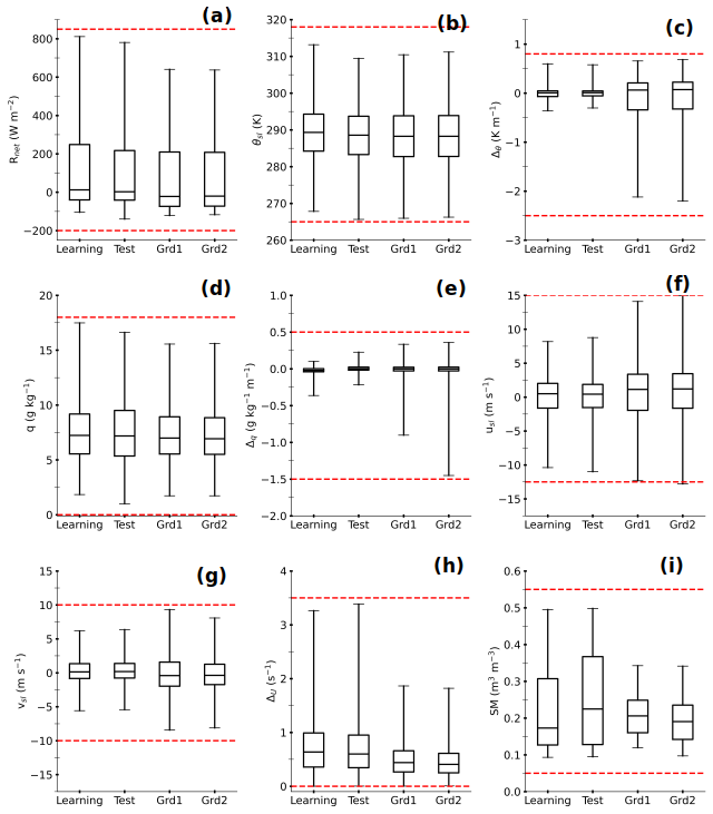
Figure A1 Box plots summarizing the interval ranges of the nine physical variables used as input to our MLP-based statistical model (Table 2). The corresponding datasets are indicated on the x axis. The whiskers represent the minimum and maximum values of each dataset. The horizontal dashed red lines indicate the extreme values used for scaling.

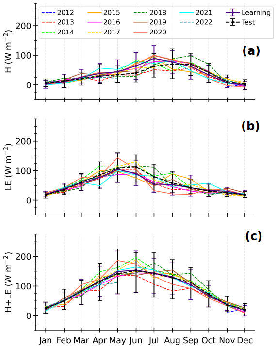
Figure A2 Composite monthly averages of observed sensible heat flux (H, a), latent heat flux (LE, b), and total turbulent heat flux (H+LE, c) for each year included in the observational data, calculated from the daily averages of half-hourly samples. The years of learning and test sets are in solid and dashed lines respectively. The thick lines correspond to the means on each subset, and the error represents the 10th and 90th percentiles.

Figure A3 Same as in Fig. 11 but for Grd2.

Figure A4 Same as in Fig. 12 but for Grd2.

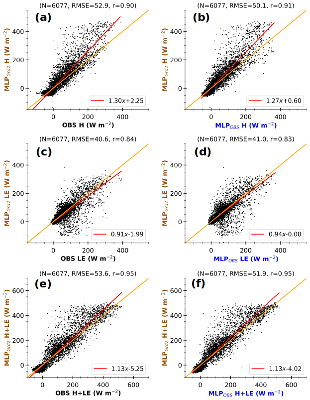
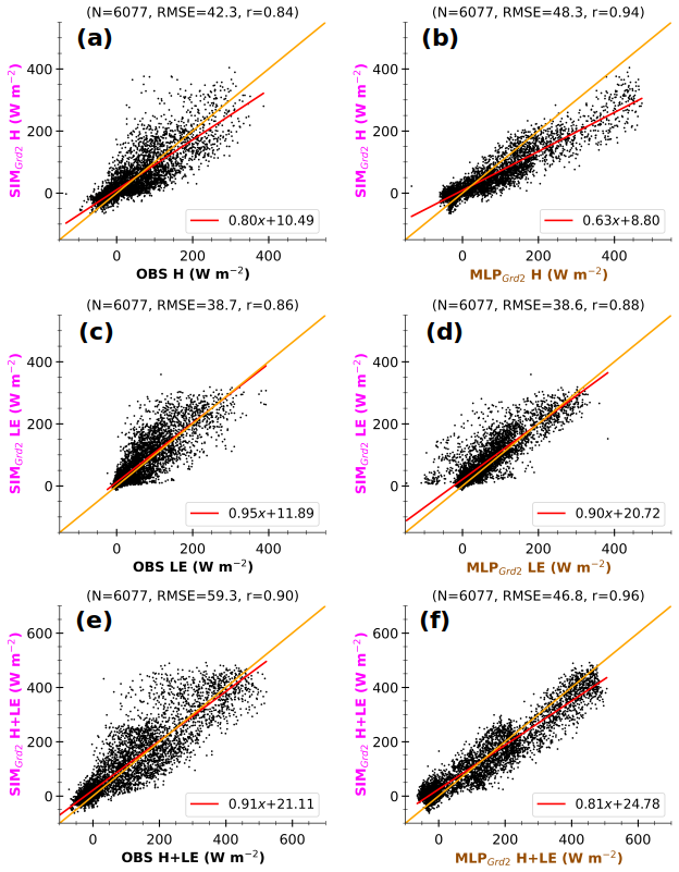
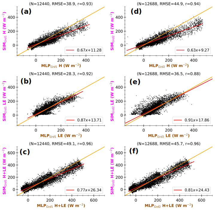
Figure A5 The 3 h simulated sensible heat flux (H, a, d), latent heat flux (LE, b, e), and total turbulent heat flux (H+LE, c, f) at Grd1 (a–c) and Grd2 (d–f) against corresponding MLP-based estimates in the simulated environment. All selected timestamps from 1 January 2012 to 31 December 2016 are considered here. The values at the top of each panel correspond to the number of samples (N), root mean square error (RMSE), and Pearson's correlation coefficient (r). The lines in red and orange represent the linear and ideal fits respectively. The axis labels are colored according to the schematic illustration in Fig. 1.

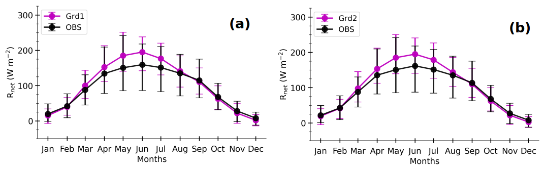
Figure A6 Composite monthly averages of simulated surface net radiative flux (R_net, magenta lines) at Grd1 (a) and Grd2 (b) and those of their respective observations at Météopole (black lines). They are computed as in Fig. 13.

Figure A7 Same as in Fig. A6 but for soil wetness (SM).

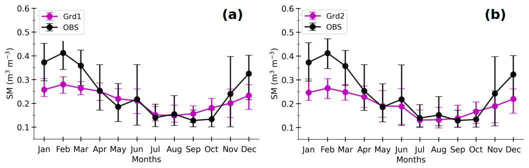
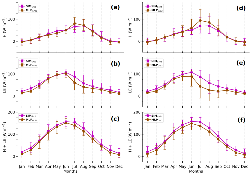
Figure A8 Composite monthly averages of simulated H (a, d), LE (b, e), and H+LE (c, f) at Grd1 and Grd2 (SIM_Grd1 and SIM_Grd2, lines in magenta) together with those of MLP-based estimates under the simulated environment (MLP_Grd1 and MLP_Grd2, lines in brown). The solid lines correspond to the means, and the error bars represent the 10th and 90th percentiles, calculated by gathering daily averages of 3 h data. All selected diurnal cycles from 1 January 2012 to 31 December 2016 are considered here.