Pochva: a new hydro-thermal process model in soil, snow, and vegetation for application in atmosphere numerical models

This work presents the land model Pochva. Pochva is a model of hydro-thermal processes at the Earth's surface and in the underlying medium. The model simulates the main hydro-thermal parameters of the surface, soil layer, vegetation, and snow cover. The soil process scheme accounts for diversity in the vertical profile of the soil physical parameters. The snow cover is processed in a multilayer scheme and its numerical algorithm allows solutions for both extremely thin and extremely thick layer cases. The model is characterized by a particular accuracy in simulating the water phase transitions in soil and snow and by the autonomy in the determination of the lower boundary condition in the soil column. The model can be used as a stand-alone land surface model driven by observed or analytical forcing data or coupled to an atmospheric model, which is either global or limited-area, in either the forecast regime or climatic regime. The results of coupling Pochva to the numerical weather prediction limited-area model Bolam are presented.

1 Introduction

Water mass balance and energy balance at the Earth's surface are key processes in the numerical modelling of the atmosphere. Such surface processes affect the conditions at the lower boundary for the main atmospheric parameters as well as the air parameters in the surface layer. The surface hydro-thermal conditions are simulated by a scheme (or model) of hydro-thermal processes at the surface and inside the underlying media, composed by the soil layer, possibly covered by vegetation, and by a snow layer.

The modelling of hydro-thermal processes in the underlying media evolved significantly from a simple soil scheme (e.g. Deardorff, 1978) to complex vegetation structures with multilayer soil hydrology and energy and multilayer snow. Examples of currently used land surface schemes include the interaction soil–biosphere–atmosphere (ISBA) model (Noilhan and Planton, 1989); the Canadian Land Surface Scheme (CLASS) (Verseghy, 1991; Verseghy et al., 1993); the Tiled ECMWF Scheme for Surface Exchanges over Land (TESSEL) model (Viterbo and Beljaars, 1995), including a multilayer snow scheme (Arduini et al., 2019); the NOAH model (Ek et al., 2003); the Common Land Model of the National Center of Atmospheric Research (USA) and Sun Yat-sen University (China) (Dai et al., 2003); the Community Land Model (CLM) (Oleson et al., 2010); the Joint UK Land Environment Simulator (JULES) (Best et al., 2011); and the GEOtop (Endrizzi et al., 2014) model. Santanello et al. (2018) provided a thorough discussion of the processes occurring between the atmosphere and the land surface and their important role in the numerical modelling of the atmosphere.

The large number and variety of existing models reflect the particular focus of several different processes occurring for the soil and the vegetation. Such differences are related to the different purposes of their application: weather prediction, study of atmospheric processes, simulation of snow cover and avalanche prediction, and climate simulations coupled with biosphere models. Some models pay particular attention to hydro-thermal exchange processes in the soil, take into account phase transition processes in soil water and processes in the snow layer, and accurately describe the fluxes at the soil surface. These models are more suitable for application in modelling atmospheric processes and weather forecasting. Other models pay more attention to an accurate description of the processes related to vegetation, distinguishing between high and low vegetation, simulating, in detail, processes like evapotranspiration, and providing an accurate simulation of carbon cycle. These models are more suited to climate and Earth system modelling.

The model proposed in the present work is closer to the first class of models, i.e. more suitable for models targeted at the study of atmospheric process and weather prediction models. In the proposed model, special attention is paid to the following aspects: the accuracy of the description of heat and moisture exchange in the soil, including the water phase transitions; the accuracy and reliability in the description of processes in the snow cover (including water melting and re-freezing); the inhomogeneity in soil parameters along the vertical; the definition of thermal and hydraulic conductivity in the soil; the definition of the air humidity at the contact surface with the soil and vegetation leaves; and the problem of determining the albedo and density of snow cover depending on its previous state. In the proposed land model, an original method is employed for the definition of the bottom boundary conditions for temperature and humidity, making the scheme autonomous within the context of a known climatology or climatological drift. The model can also be useful for the simulation of snow cover for avalanche prediction purposes since the snow module is independent of the other modules and can be applied separately. Pochva can also be used with a forcing derived from observational data for defining the fluxes between the surface and the atmosphere as well as for idealized column simulations.

The present paper is divided into eight sections. Sections 2 to 6 describe the numerical schemes included in the Pochva, indeed surface processes, processes in the vegetation, heat exchange processes in the soil, moisture exchange processes in the soil, and processes in the snow layer. Section 7 and the Appendix contain the description of the numerical experiments and their results. Section 8 summarizes the conclusions and discusses some critical points of the land model and some issues on the verification results.

2 Surface processes scheme

In the atmospheric numerical modelling, the interaction between the atmosphere and the Earth's surface involves mainly fluxes of heat and moisture. The thermal state of the soil environment in the present model is synthesized by entropy as it simplifies the description of the water phase changes following the idea proposed in Pressman (1994).

The state of the atmosphere in interaction with the Earth's surface is described by air temperature, specific humidity and pressure at the lowest atmospheric level, turbulent transfer coefficients between the surface and lowest atmospheric level, total net radiation flux, and fluxes of atmospheric precipitation in liquid and crystal phases. The thermodynamic state of the surface is described by two parameters, temperature and specific humidity of the air at the surface. The values of these two parameters depend on the whole state of the underlying surface.

2.1 State of the soil surface

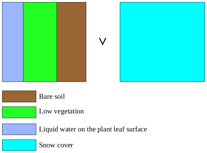
According to the principles adopted in this work, a unit size of underlying surface is composed by a set of fractional contributions, each of which exhibits uniform characteristics from the point of view of interaction with the atmosphere. The soil surface cover can be characterized by vegetation (grass, shrub, trees, woodland) and snow. Snow cover and vegetation imply the presence of a particular layer with its own thermodynamic characteristics, which thus has a distinct temperature. For this reason, it is not possible to classify these surface categories as a fraction of the surface of the soil itself, but it is necessary to consider them as independent “columns”. As a consequence, if we introduce the concept of fraction of snow cover, it is necessary to divide the surface into three independent columns, each with its own temperature even in the case of equal upper and lower boundary conditions. In the present version of the land model, however, the following simplifying assumptions have been made: the vegetation is not a special medium, but it is considered a part of the soil surface with particular characteristics; the snow layer can either cover the entire grid cell surface or not exist at all, and a fractional snow cover is introduced only as a diagnostic field to allow for the computation of the radiative characteristics of the surface (albedo, emissivity). Under these assumptions, the soil surface can consist of bare soil possibly partly covered by vegetation, which in turn may be partly covered by water or snow. These two features of the surface are assumed as they cannot exist simultaneously.

Figure 1 Scheme of the soil surface.

For each area of a single model grid cell, the vegetation fraction is determined by an external vegetation parameter dataset. The fraction of vegetation leaves covered by water is determined by the ratio between the water mass deposited on the leaf surface and the maximum value of this mass, which is also evaluated using a dataset.

Then the fractional surface interacting with atmosphere can be, without snow cover (F_snow=0)

• 1.

  $F_{\mathrm{baresoil}}=\mathrm{1}-F_{\mathrm{veg}}$, bare soil;

• 2.

  $F_{\mathrm{veg}}^{\mathrm{dry}}=F_{\mathrm{veg}}\cdot \left(\mathrm{1}-F_{\mathrm{veg}}^{\text{leaf wet}}\right)$, vegetation leaves not covered by water;

• 3.

  $F_{\mathrm{veg}}^{\mathrm{wet}}=F_{\mathrm{veg}}\cdot F_{\mathrm{veg}}^{\text{leaf wet}}$, vegetation leaves covered by water.

In the case of snow cover, under the indicated assumptions the only type of interacting surface is F_snow=1.

More precisely, in the presence of snow, we always assume F_snow=1 for the computation of moisture fluxes, while for the entropy fluxes, F_snow=1 holds only if the snow cover has a minimal thickness; otherwise, for a thin snow layer, entropy fluxes are computed under the assumption of F_snow=0.

For each of these four surface types, surface air temperature and humidity have to be defined. The overall surface air temperature and humidity for the whole grid cell are then computed as a weighted average, where each weight equals the fractional area for each surface type.

2.2 Air temperature and humidity on bare soil

For bare soil, the surface air temperature (T_{surf soil}) is equal to the temperature of the upper soil layer (T_{soil 0}). The air specific humidity, q_{v surf soil} (kg kg⁻¹) is defined according to the diagnostic expression

$$\begin{array}{}\text{(1)}& q_{\text{v surf soil}}=q_{\text{v atm 1}}\cdot \left(\mathrm{1}-{\mathit{\alpha }}_{\mathrm{soil}}\right)+q_{\text{v sat}}\left(T_{\text{soil 0}}\right)\cdot {\mathit{\alpha }}_{\mathrm{soil}},\end{array}$$

where q_{v atm 1} is the air specific humidity at the lowest atmospheric level (kg kg⁻¹); q_{v sat} (T_{soil 0}) is the saturation air specific humidity at temperature T_{soil 0} computed as

$$\begin{array}{}\text{(2)}& q_{\text{v sat}}=\left\{\begin{array}{l}{q}_{\text{v sat}}^{\mathrm{water}}\left(T_{\text{soil 0}}\right),\text{ if }{T}_{\text{soil 0}}⩾T_{\mathrm{0}}\\ q_{\text{v sat}}^{\text{ice}}\left(T_{\text{soil 0}}\right),\text{ if }{T}_{\text{soil 0}}<T_{\mathrm{0}}\end{array}\right.,\end{array}$$

where q_{v sat water} and q_{v sat ice} are saturation air specific humidity over liquid water and ice respectively, α_soil is an empirical coefficient, and T₀=273.15 (K) is constant.

For the definition of the empirical coefficient α_soil, an original method is proposed in this work. The approach is based on Kondo et al. (1990) using both concepts of turbulent exchange and influence of top soil moisture to surface air humidity. Various empirical parameters have been introduced by the author and presented in Eqs. (3), (4), and (5). These formulations and the values of parameters are the results of many numerical experiments and statistical verification on a big number of observational meteorological stations (see Sect. 7). The definition is the following:

$$\begin{array}{}\text{(3)}& {\mathit{\alpha }}_{\mathrm{soil}}={\displaystyle \frac{\mathrm{2}\cdot F_{\mathrm{2}}^{\mathrm{soil}}}{e^{F_{\mathrm{1}}^{\mathrm{soil}}{K}_{\mathrm{v}}^{\mathrm{turb}}}+e^{-F_{\mathrm{1}}^{\mathrm{soil}}{K}_{\mathrm{v}}^{\mathrm{turb}}}}},\end{array}$$

where $K_{\mathrm{v}}^{\mathrm{turb}}$ is the coefficient of water vapour turbulent exchange in the lowest 1 m of the surface layer (m² s⁻¹),

$F_{\mathrm{1}}^{\mathrm{soil}}$ and $F_{\mathrm{2}}^{\mathrm{soil}}$ are empirical functions of the relative moisture contents of the upper soil layer:

$$\begin{array}{}\text{(4)}& {\displaystyle }{F}_{\mathrm{1}}^{\mathrm{soil}}=\mathrm{7}\cdot \left[\mathrm{2}+\mathrm{3}\cdot {\left(\mathrm{1}-q_{\mathrm{0}}^{\mathrm{rel}}\right)}^{\mathrm{0.2}+\mathrm{0.05}\cdot b}\right],\text{(5)}& {\displaystyle }{F}_{\mathrm{2}}^{\mathrm{soil}}=\mathrm{1}-\mathrm{0.8}\cdot {\left(\mathrm{1}-q_{\mathrm{0}}^{\mathrm{rel}}\right)}^{\mathrm{0.2}+\mathrm{0.05}\cdot b},\end{array}$$

where b is the so-called soil exponent (Clapp and Hornberger, 1978) and $q_{\mathrm{0}}^{\mathrm{rel}}$ is the soil relative water content at the top level (see Sect. 4). The choice of the values defining the empirical function is crucial since it strongly influences the magnitude of the water vapour flux and its associated latent heat flux, which, in turn, influences the soil surface temperature and the air temperature at 2 m that are routinely used for the verification of numerical weather predictions. The methodology used for the definition of the empirical coefficients and their influence on the numerical weather forecast will be discussed in a separate publication dedicated to the evaluation of the numerical model results.

2.3 Air temperature and humidity over vegetation with leaves not covered by water

The air temperature in this case ($T_{\mathrm{veg}}^{\mathrm{dry}}$) is equal to the temperature of the topmost soil layer (T_{soil 0}). For the definition of air humidity, we distinguish between two cases: the evapotranspiration being active or not active. The conditions under which evapotranspiration is or is not active are shown in Sect. 3.

The method of numerical approximation of evapotranspiration presented here has been formulated using the approach presented in Pressman (1994).

In the case of a lack of evapotranspiration, the air humidity is equal to the air humidity at the lowest atmospheric layer, while in the case of active evapotranspiration by leaves not covered by water, it is defined analogously to the case of bare soil:

$$\begin{array}{}\text{(6)}& \begin{array}{rl}& q_{\text{v veg}}^{\mathrm{dry}}=\\ & \left\{\begin{array}{l}{q}_{\text{v atm}},\text{ if evapotranspiration is not active}\\ q_{\text{v atm}}\cdot \left(\mathrm{1}-{\mathit{\alpha }}_{\mathrm{veg}}\cdot {\mathit{\beta }}_{\mathrm{veg}}\right)+q_{\text{v sat}}\left(T_{\text{soil 0}}\right)\cdot {\mathit{\alpha }}_{\mathrm{veg}}\\ \cdot {\mathit{\beta }}_{\mathrm{veg}},\text{ if evapotranspiration is active}\end{array}\right.,\end{array}\end{array}$$

where $q_{\text{v veg}}^{\mathrm{dry}}$ is the air specific humidity over respiring plant leaf, q_{v atm} is air specific humidity at the bottom atmospheric level (kg kg⁻¹), q_{v sat}(T_{soil 0}) is saturation air specific humidity (kg kg⁻¹) at soil surface temperature T_{soil 0} (see Sect. 2.2), α_veg is an empirical parameter depending on the magnitude of the evapotranspiration activity, and β_veg is a parameter depending on the moisture content in the root layer of the soil (the definition of this parameter is given by Eqs. 11–13; see below).

The approximation of the parameter defining the evapotranspiration activity is similar to the method presented by Eq. (3). The parameter is given by

$$\begin{array}{}\text{(7)}& {\mathit{\alpha }}_{\mathrm{veg}}={\displaystyle \frac{\mathrm{2}\cdot F_{\mathrm{2}}^{\mathrm{veg}}}{e^{F_{\mathrm{1}}^{\mathrm{veg}}\cdot K_{\mathrm{v}}^{\mathrm{turb}}}+e^{-F_{\mathrm{1}}^{\mathrm{veg}}\cdot K_{\mathrm{v}}^{\mathrm{turb}}}}},\end{array}$$

where $F_{\mathrm{1}}^{\mathrm{veg}}$ and $F_{\mathrm{2}}^{\mathrm{veg}}$ are empirical functions depending on the turbulent exchange coefficients for water vapour in the lowest 1 m of the atmospheric surface layer and on the intensity of the evapotranspiration process, which in turn depends on the flux of incoming visible solar radiation and on the LAI (leaf area index) following the concept proposed in (Viterbo and Beljaars, 1995) according to

$$\begin{array}{}\text{(8)}& {\displaystyle }{F}_{\mathrm{1}}^{\mathrm{veg}}=\mathrm{30}\cdot \left[-\mathrm{1.9}\cdot {\displaystyle \frac{\mathrm{LAI}}{{\mathrm{LAI}}_{max}}}+\mathrm{2}\right],\text{(9)}& {\displaystyle }{F}_{\mathrm{2}}^{\mathrm{veg}}=min\left[{\left[min\left({\displaystyle \frac{F_{\text{rad vis}}}{\mathrm{600}}},\mathrm{1}\right)\right]}^{\mathrm{0.3}},{\left({\displaystyle \frac{\mathrm{LAI}}{{\mathrm{LAI}}_{max}}}\right)}^{\mathrm{0.2}}\right],\end{array}$$

where F_{rad vis} is the flux of visible solar radiation at the surface (W m⁻²) and LAI_max is the maximum value of LAI in the static global database used.

In this case, as in the case of air surface humidity over bare soil, the various empirical parameters in Eqs. (7), (8), and (9) have been introduced by the author, and their values have been obtained as a result of many numerical experiments and statistical verification.

In order to evaluate the parameter β_veg, a description of the finite-difference representation of the vertical space coordinate used in the model is described here.

As a vertical coordinate, the geometrical length (depth) is used, with the origin positioned at the surface and values increasing with depth. The vertical computational domain is divided into full and half levels, with the upper full level having the index 0, and with each half level having the same index as the full level located below it; the level indices increase with depth (see Fig. 2).

Figure 2 Finite-difference discretization of the vertical coordinate in the soil.

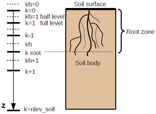
The upper part of the soil column may contain plant roots. The depth of the root layer is defined as

$$\begin{array}{}\text{(10)}& Z_{\mathrm{root}}={\sum }_{k=\mathrm{0}}^{k_{\mathrm{root}}}\left(z_{kh+\mathrm{1}}-z_{kh}\right),\end{array}$$

where z (m) is the space coordinate in soil, k is the index of full level in the vertical discretization, and k_root is the index of the deepest root zone level. The root zone depth is defined using a suitable vegetation dataset. In this work, the distribution of vertical soil levels is not uniform; the thickness of soil layers increases with depth according to an exponential law, but it is possible to apply any other distribution. The depth of the soil bottom in the present scheme may be different for water exchange processes and for thermal exchange processes, depending on bottom boundary conditions, and they may differ from one geographical location to another according to the local geographical characteristics.

$$\begin{array}{}\text{(11)}& {\displaystyle }{\mathit{\beta }}_{\mathrm{veg}}={\displaystyle \frac{{\sum }_{k=\mathrm{0}}^{k_{\mathrm{root}}}\left(z_{\mathrm{kh}+\mathrm{1}}-z_{kh}\right)\cdot F\left(q_k^{\mathrm{rel}}\right)}{Z_{\mathrm{root}}}},\text{(12)}& {\displaystyle }F\left(q_k^{\mathrm{rel}}\right)=\left\{\begin{array}{l}\mathrm{1},\text{ if }{q}_k^{\mathrm{rel}}⩾q_k^{\text{rel ref}}\\ \frac{q_k^{\mathrm{rel}}-q_k^{\text{rel wilt}}}{q_k^{\text{rel ref}}-q_k^{\mathrm{rel}}},\text{ if }{q}_k^{\text{rel wilt}}<q_k^{\mathrm{rel}}<q_k^{\text{rel ref}}\\ \mathrm{0},\text{ if }{q}_k^{\mathrm{rel}}⩽q_k^{\text{rel wilt}}\end{array}\right.,\text{(13)}& {\displaystyle }\begin{array}{rl}{q}_k^{\mathrm{rel}}& ={\displaystyle \frac{q_k-q_k^{min}}{q_k^{max}-q_k^{min}}},q_k^{\text{rel wilt}}={\displaystyle \frac{q_k^{\mathrm{wilt}}-q_k^{min}}{q_k^{max}-q_k^{min}}},\\ & q_k^{\text{rel ref}}={\displaystyle \frac{q_k^{\mathrm{ref}}-q_k^{min}}{q_k^{max}-q_k^{min}}},\end{array}\end{array}$$

where q_k and $q_k^{\mathrm{rel}}$ are the soil specific volumetric (m³ m⁻³) and relative (proportion) water content at level k; $q_k^{\max }$ and $q_k^{min}$ are the maximum and minimum soil specific volumetric content at level k (m³ m⁻³); $q_k^{\mathrm{wilt}}$ and $q_k^{\text{rel wilt}}$ are soil specific volumetric (m³ m⁻³) and relative (proportion) water content at level k at wilting point, i.e. at the water content at which plant evapotranspiration stops because of overly dry soil; and $q_k^{\mathrm{ref}}$ and $q_k^{\text{rel ref}}$ are soil specific volumetric (m³ m⁻³) and relative (proportion) water content at level k at reference point, i.e. at the water content level at which plant evapotranspiration stops increasing because of highly wet soil.

2.4 Air temperature and humidity over vegetation with leaves covered by water

The air temperature in this case ($T_{\mathrm{veg}}^{\mathrm{wet}}$) is equal to the temperature of the topmost soil layer (T_{soil 0}). The air humidity is equal to the saturation humidity at the given temperature:

$$\begin{array}{}\text{(14)}& q_{\text{v veg}}^{\mathrm{wet}}=q_{\text{v sat}}\left(T_{\text{soil 0}}\right),\end{array}$$

where q_vsat(T_{soil 0}) is the saturation air specific humidity (kg kg⁻¹) at soil surface temperature T_{soil 0} (see Sect. 2.2).

2.5 Air temperature and humidity over snow cover

The air temperature in this case (T_{surf snow}) is equal to the temperature of the topmost snow layer (T_snow 0). The air humidity is equal to the saturation humidity at the given temperature:

$$\begin{array}{}\text{(15)}& q_{\text{v surf snow}}=q_{\text{v sat}}\left(T_{\text{snow 0}}\right),\end{array}$$

where q_{v sat}(T_snow 0) is the saturation air specific humidity (kg kg⁻¹) at snow cover surface temperature T_snow 0.

$$\begin{array}{}\text{(16)}& q_{\text{v sat}}=\left\{\begin{array}{l}{q}_{\text{v sat}}^{\mathrm{water}}\left(T_{\text{snow 0}}\right),\text{ if }{T}_{\text{snow 0}}⩾T_{\mathrm{0}}\\ q_{\text{v sat}}^{\mathrm{ice}}\left(T_{\text{snow 0}}\right),\text{ if }{T}_{\mathrm{snow}\mathrm{0}}<T_{\mathrm{0}}\end{array}\right.,\end{array}$$

where $q_{\text{v sat}}^{\mathrm{water}}$ and $q_{\text{v sat}}^{\mathrm{ice}}$ are saturation air specific humidity (kg kg⁻¹) at snow cover surface temperature T_{snow 0} over liquid water and over ice respectively.

2.6 Air temperature and humidity over a composite soil surface

Having defined the values of air temperature and humidity over all the possible components of a composite soil surface and knowing the fraction of each component of the surface, it is possible to define the overall surface air temperature (T_surf) and humidity (q_{v surf}).

In the absence of snow cover, or in the presence of a so-called shallow snow layer (see the description of snow scheme), the overall surface air temperature is equal to the weighted mean of the temperatures of the surface components:

$$\begin{array}{}\text{(17)}& T_{\mathrm{surf}}=T_{\text{surf soil}}\cdot F_{\mathrm{baresoil}}+T_{\mathrm{veg}}^{\mathrm{dry}}\cdot F_{\mathrm{veg}}^{\mathrm{dry}}+T_{\mathrm{veg}}^{\mathrm{wet}}\cdot F_{\mathrm{veg}}^{\mathrm{wet}},\end{array}$$

while in the case of a thick snow layer, we have

$$\begin{array}{}\text{(18)}& T_{\mathrm{surf}}=T_{\text{surf snow}}.\end{array}$$

Similar formulae hold for the surface specific humidity in the case of absence of snow cover:

$$\begin{array}{}\text{(19)}& q_{\text{v surf}}=q_{\text{v surf soil}}\cdot F_{\mathrm{baresoil}}+q_{\text{v veg}}^{\mathrm{dry}}\cdot F_{\mathrm{veg}}^{\mathrm{dry}}+q_{\text{v veg}}^{\mathrm{wet}}\cdot F_{\mathrm{veg}}^{\mathrm{wet}},\end{array}$$

and in the presence of snow cover (either thick or shallow), where it is

$$\begin{array}{}\text{(20)}& q_{\text{v surf}}=q_{\text{v surf snow}}.\end{array}$$

2.7 Entropy flux between soil surface and atmosphere

The surface incoming entropy flux is composed by the turbulent flux of entropy for dry air, the turbulent flux of entropy due to water vapour, and the entropy flux due to global radiation:

$$\begin{array}{}\text{(21)}& {\mathrm{\Phi }}_{S\text{surf}}={\mathrm{\Phi }}_{\text{S rad}}+{\mathrm{\Phi }}_{{\mathrm{S}}_{\mathrm{da}}}^{\mathrm{turb}}+{\mathrm{\Phi }}_{{\mathrm{S}}_{\mathrm{v}}}^{\mathrm{turb}},\end{array}$$

where Φ_S surf is the surface entropy flux (J K⁻¹ m⁻² s⁻¹), ${\mathrm{\Phi }}_{\text{S da}}^{\mathrm{turb}}$ and ${\mathrm{\Phi }}_{\text{S v}}^{\mathrm{turb}}$ are the entropy fluxes originating from the turbulent entropy flux of dry air and of water vapour (J K⁻¹ m⁻² s⁻¹), and Φ_{S rad} is the entropy flux originating from global radiation (J K⁻¹ m⁻² s⁻¹).

The flux of entropy due to the flux of water (in liquid and solid phases) from atmospheric precipitation is neglected since, in the soil entropy scheme, the entropy flux originating from soil moisture flux is also neglected.

The entropy fluxes are computed according to the following relations:

$$\begin{array}{}\text{(22)}& {\mathrm{\Phi }}_{\text{S rad}}={\displaystyle \frac{{\mathrm{\Phi }}_{\mathrm{rad}}}{T_{\mathrm{surf}}}},\end{array}$$

where Φ_rad is the flux of global radiation (W m⁻²).

$$\begin{array}{}\text{(23)}& {\mathrm{\Phi }}_{{\mathrm{S}}_{\text{da surf}}}^{\mathrm{turb}}=K_{\mathrm{h}}^{\mathrm{turb}}\cdot {\mathit{\rho }}_{\text{a surf}}\cdot {\displaystyle \frac{S_{\text{da surf}}-S_{\text{da atm}}}{z_{\mathrm{atm}}}},\end{array}$$

where $K_{\mathrm{h}}^{\mathrm{turb}}$ is the coefficient of heat exchange in the surface layer (m² s⁻¹), ρ_{a surf} is the air density at the surface (kg m⁻³), and z_atm is the height of the lowest atmospheric level (m). S_{da surf} and S_{da atm} are the specific entropy of dry air on the surface and at the lowest atmospheric level (J kg⁻¹ K⁻¹).

The entropy of dry air is defined by the relation

$$\begin{array}{}\text{(24)}& S_{\mathrm{da}}=q_{\mathrm{d}}\cdot \left[C_p^{\mathrm{d}}\ln \left({\displaystyle \frac{T}{T_{\mathrm{0}}}}\right)-R_{\mathrm{d}}\ln \left({\displaystyle \frac{P_{\mathrm{d}}}{P_{\mathrm{0}}}}\right)\right],\end{array}$$

where S_da is the specific entropy of dry air (J kg⁻¹ K⁻¹), q_d is the specific mass of dry air (kg kg⁻¹), T is the temperature (K), P_d is the partial pressure of dry air (Pa), T₀=273.15 K is the reference temperature, P₀=10⁵ Pa is the reference pressure, $C_p^{\mathrm{d}}=\mathrm{1004.6}$ J kg⁻¹ K⁻¹ is the specific heat capacity of dry air at constant pressure, and R_d=287.05 J kg⁻¹ K⁻¹ is the gas constant of dry air.

In order to define the entropy of dry air at the surface and at the lowest atmospheric level, the known values of air temperature, humidity, and pressure are used together with the following relations:

$$\begin{array}{}\text{(25)}& {\displaystyle }{q}_{\text{da surf}}=\mathrm{1}-q_{\text{v surf}},\text{(26)}& {\displaystyle }{q}_{\text{da atm}}=\mathrm{1}-q_{\text{v atm}},\text{(27)}& {\displaystyle }{P}_{\text{d surf}}=P_{\text{surf}}-e_{\text{surf}},\text{(28)}& {\displaystyle }{P}_{\text{d atm}}=P_{\text{atm}}-e_{\text{atm}},\end{array}$$

where q_{da surf} and q_{da atm} are dry-air specific mass at the surface and at the lowest atmospheric level (kg kg⁻¹), P_{d surf} and P_{d atm} are the partial pressure of dry air at the surface and at the lowest atmospheric level (Pa), and e_surf and e_atm are the partial pressure of water vapour at the surface and at the lowest atmospheric level (Pa).

The entropy flux of water vapour originating from turbulent exchange in the layer between the soil surface and the lowest atmospheric level is defined as

$$\begin{array}{}\text{(29)}& {\mathrm{\Phi }}_{{\text{S}}_{\text{v}}}^{\text{turb}}=K_{\mathrm{v}}^{\mathrm{turb}}\cdot {\mathit{\rho }}_{\text{a}}\cdot {\displaystyle \frac{S_{\text{v surf}}-S_{\text{v atm}}}{z_{\text{atm}}}},\end{array}$$

where S_{v surf} and S_{v atm} are the specific entropy of water vapour at the surface and at the lowest atmospheric level respectively (J kg⁻¹ K⁻¹), which, in turn, are defined by

$$\begin{array}{}\text{(30)}& S_{\mathrm{v}}=q_{\mathrm{v}}\cdot \left[C_{\mathrm{v}}^{\mathrm{d}}\ln \left({\displaystyle \frac{T}{T_{\mathrm{0}}}}\right)-R_{\mathrm{v}}\ln \left({\displaystyle \frac{e}{e_{\mathrm{0}}}}\right)+{\displaystyle \frac{L_{\mathrm{i}}^{\mathrm{v}}}{T_{\mathrm{0}}}}\right]\end{array}$$

where S_v is the specific entropy of water vapour (J kg⁻¹ K⁻¹), q_v is the air specific humidity (kg kg⁻¹), e is the partial pressure of water vapour (Pa), e₀=611 Pa is the reference partial pressure of water vapour, $C_p^{\mathrm{v}}=\mathrm{1869.46}$ J kg⁻¹ K⁻¹ is the specific heat of water vapour at constant pressure, R_v=461.51 J kg⁻¹ K⁻¹ is the gas constant for water vapour, and $L_{\mathrm{i}}^{\mathrm{v}}=\mathrm{2}\mathrm{834}\mathrm{170.5}$ J kg⁻¹ is the specific latent heat for ice–vapour phase transition.

The total entropy flux between the atmosphere and soil surface (Φ_S surf) determined in this way has to be assigned to each component of the complex soil surface in order to define the boundary condition for each type of surface. As introduced in Sect. 2.1, the surface can be composed of soil partially covered by either low vegetation or snow, which, in turn, may be thick or shallow. From the point of view of entropy (energy) exchange, low vegetation behaves as a transparent layer; i.e. it does not have an own temperature, and it is part of the soil surface. Thus, it does not have its own entropy flux. Hence, two cases may occur.

The first case occurs when snow cover is absent or shallow. In this case, all the components of the flux fully impinge on the soil surface with low vegetation, and snow surface does not receive any flux:

$$\begin{array}{ll}{\displaystyle }& {\displaystyle }{\mathrm{\Phi }}_{S\text{surf}}^{\mathrm{soil}}={\mathrm{\Phi }}_{S\text{surf}},\\ {\displaystyle }& {\displaystyle }{\mathrm{\Phi }}_{S\text{surf}}^{\mathrm{snow}}=\mathrm{0}.\end{array}$$

The second case occurs when the snow layer is present and thick. In this case, all of the entropy flux impinges on the snow surface, and the soil surface does not receive any direct flux:

$$\begin{array}{ll}{\displaystyle }& {\displaystyle }{\mathrm{\Phi }}_{S\text{surf}}^{\mathrm{soil}}=\mathrm{0},\\ {\displaystyle }& {\displaystyle }{\mathrm{\Phi }}_{S\text{surf}}^{\mathrm{snow}}={\mathrm{\Phi }}_{S\text{surf}}.\end{array}$$

2.8 Water vapour flux between soil and atmosphere

The flux of water vapour originating by means of turbulent exchange between the surface and the atmosphere is defined as

$$\begin{array}{}\text{(31)}& {\mathrm{\Phi }}_{\mathrm{v}}^{\mathrm{turb}}=K_{\mathrm{v}}^{\mathrm{turb}}\cdot {\mathit{\rho }}_{\text{a surf}}\cdot {\displaystyle \frac{q_{\text{v surf}}-q_{\text{v atm}}}{z_{\mathrm{atm}}}},\end{array}$$

where ${\mathrm{\Phi }}_{\mathrm{v}}^{\mathrm{turb}}$ is the flux of water vapour in the atmosphere surface layer (kg m⁻² s⁻¹).

This summary flux has to be split between the components of the soil surface.

In the absence of snow cover, the water vapour exchange takes place between the atmosphere and the soil surface covered by (partly wet) vegetation. We can distinguish between two cases: in the first case, the flux is positive (i.e. downward), and thus condensation (deposition) of water vapour on the surface takes place; in the second case, the flux is negative (i.e. upward), and thus evaporation (sublimation) from the surface takes place.

When the flux is directed downward, it partly impinges on the bare soil surface and partly on the vegetation, where it contributes to the formation of dew over the leaves up to a maximum pre-specified value of water content as in the following formulae:

$$\begin{array}{}\text{(32)}& {\displaystyle }{\mathrm{\Phi }}_{\text{v soil}}^{\mathrm{turb}}={\mathrm{\Phi }}_{\mathrm{v}}^{\mathrm{turb}}\cdot \left(\mathrm{1}-F_{\mathrm{veg}}\right),\text{(33)}& {\displaystyle }{\mathrm{\Phi }}_{\text{v veg dry}}^{\mathrm{turb}}=\mathrm{0},\text{(34)}& {\displaystyle }{\mathrm{\Phi }}_{\text{v veg wet}}^{\mathrm{turb}}=min\left\{{\mathrm{\Phi }}_{\mathrm{v}}^{\mathrm{turb}}\cdot F_{\mathrm{veg}},{\displaystyle \frac{q_{\text{w veg}}^{max}-q_{\text{w veg}}}{\mathrm{\Delta }t}}\right\},\end{array}$$

where ${\mathrm{\Phi }}_{\text{v soil}}^{\mathrm{turb}}$ is the flux of water vapour in the atmospheric surface layer towards bare soil (kg m⁻² s⁻¹), ${\mathrm{\Phi }}_{\text{v veg dry}}^{\mathrm{turb}}$ and ${\mathrm{\Phi }}_{\text{v veg wet}}^{\mathrm{turb}}$ are the fluxes of water vapour in the atmospheric surface layer towards vegetation that is not moistened and that is moistened (kg m⁻² s⁻¹), q_{w veg} and $q_{\text{w veg}}^{\max }$ are the water content of plant leaves and its maximum value (kg m⁻²) respectively, and Δt is the model time step (s).

When the flux is directed upward, it removes water partly from the bare soil surface, partly from the soil through plant evapotranspiration, and partly through evaporation of water on the leaves. When conditions for evapotranspiration are not met, the corresponding flux is zero (see description of vegetation scheme), while evaporation from leaves obviously occurs as long as there is water available on leaf surface, as in the following formulae:

$$\begin{array}{}\text{(35)}& {\displaystyle }\begin{array}{rl}& {\mathrm{\Phi }}_{\text{v veg dry}}^{\mathrm{turb}}=\\ & \left\{\begin{array}{l}{\mathrm{\Phi }}_{\mathrm{v}}^{\mathrm{turb}}\cdot F_{\mathrm{veg}}^{\mathrm{dry}},\text{if evapotranspiration is possible}\\ \mathrm{0},\text{if evapotranspiration is not possible}\end{array}\right.,\end{array}\text{(36)}& {\displaystyle }{\mathrm{\Phi }}_{\text{v veg wet}}^{\mathrm{turb}}=max\left\{{\mathrm{\Phi }}_{\mathrm{v}}^{\mathrm{turb}}\cdot F_{\mathrm{veg}}^{\mathrm{wet}},{\displaystyle \frac{-q_{\text{w veg}}}{\mathrm{\Delta }t}}\right\},\text{(37)}& {\displaystyle }{\mathrm{\Phi }}_{\text{v soil}}^{\mathrm{turb}}={\mathrm{\Phi }}_{\mathrm{v}}^{\mathrm{turb}}-{\mathrm{\Phi }}_{\text{v veg dry}}^{\mathrm{turb}}-{\mathrm{\Phi }}_{\text{v veg wet}}^{\mathrm{turb}}.\end{array}$$

In the presence of snow cover, the water vapour fluxes between the atmosphere and the bare soil/vegetation are null, and the interaction takes place only between the atmosphere and the snow layer:

$$\begin{array}{}\text{(38)}& {\mathrm{\Phi }}_{\text{v snow}}^{\mathrm{turb}}={\mathrm{\Phi }}_{\mathrm{v}}^{\mathrm{turb}},\end{array}$$

where ${\mathrm{\Phi }}_{\text{v snow}}^{\mathrm{turb}}$ is the flux of water vapour in the atmosphere surface layer towards the snow layer (kg m⁻² s⁻¹).

2.9 Atmospheric precipitation flux at the surface

Atmospheric precipitation flux over surface, divided into liquid (${\mathrm{\Phi }}_{\mathrm{w}}^{\mathrm{liq}}$) and solid (${\mathrm{\Phi }}_{\mathrm{w}}^{\mathrm{ice}}$), is provided by the atmospheric model. The distribution of these fluxes over the soil surface depends on the presence of snow over it.

In the absence of snow cover, liquid precipitation contributes to the surface components, including leaves, according to the fraction of each component; the amount of water on leaves exceeding the maximum allowable is immediately redistributed among the bare soil components:

$$\begin{array}{}\text{(39)}& {\displaystyle }{\mathrm{\Phi }}_{\text{w veg}}^{\mathrm{liq}}=min\left\{{\mathrm{\Phi }}_{\mathrm{w}}^{\mathrm{liq}}\cdot F_{\mathrm{veg}},{\displaystyle \frac{q_{\text{w veg}}^{max}-q_{\text{w veg}}}{\mathrm{\Delta }t}}\right\},\text{(40)}& {\displaystyle }{\mathrm{\Phi }}_{\text{w soil}}^{\mathrm{liq}}={\mathrm{\Phi }}_{\mathrm{w}}^{\text{liq}}-{\mathrm{\Phi }}_{\text{w veg}}^{\mathrm{liq}},\text{(41)}& {\displaystyle }{\mathrm{\Phi }}_{\text{w snow}}^{\mathrm{liq}}=\mathrm{0},\end{array}$$

where ${\mathrm{\Phi }}_{\mathrm{w}}^{\mathrm{liq}}$, ${\mathrm{\Phi }}_{\text{w soil}}^{\mathrm{liq}}$, ${\mathrm{\Phi }}_{\text{w veg}}^{\mathrm{liq}}$, and ${\mathrm{\Phi }}_{\text{w snow}}^{\mathrm{liq}}$ are the fluxes of atmospheric precipitation in the liquid phase on the whole surface, the soil surface, vegetation, and the snow-covered surface respectively (kg m⁻² s⁻¹).

In the presence of snow cover, all of the liquid precipitation flux is directed towards the snow layer:

$$\begin{array}{}\text{(42)}& {\displaystyle }{\mathrm{\Phi }}_{\text{w soil}}^{\mathrm{liq}}={\mathrm{\Phi }}_{\text{w veg}}^{\mathrm{liq}}=\mathrm{0},\text{(43)}& {\displaystyle }{\mathrm{\Phi }}_{\text{w snow}}^{\mathrm{liq}}={\mathrm{\Phi }}_{\mathrm{w}}^{\mathrm{liq}}.\end{array}$$

Conversely, the solid precipitation flux is always directed towards snow layer, creating it if it does not exist:

$$\begin{array}{}\text{(44)}& {\displaystyle }{\mathrm{\Phi }}_{\text{w snow}}^{\mathrm{ice}}={\mathrm{\Phi }}_{\mathrm{w}}^{\mathrm{ice}},\text{(45)}& {\displaystyle }{\mathrm{\Phi }}_{\text{w soil}}^{\mathrm{ice}}={\mathrm{\Phi }}_{\text{w veg}}^{\mathrm{ice}}=\mathrm{0}.\end{array}$$

where ${\mathrm{\Phi }}_{\mathrm{w}}^{\mathrm{ice}}$, ${\mathrm{\Phi }}_{\text{w snow}}^{\mathrm{ice}}$, ${\mathrm{\Phi }}_{\text{w soil}}^{\mathrm{ice}}$, and ${\mathrm{\Phi }}_{\text{w veg}}^{\mathrm{ice}}$ are the fluxes of atmospheric precipitation in the solid phase on the whole surface, the snow-covered surface, the snow-free soil surface, and vegetation respectively (kg m⁻² s⁻¹).

The surface process scheme defines the conditions on the upper layer of the soil column in the absence of snow cover or on the snow column in the presence of snow. The boundary conditions are given by fluxes of entropy and water, which can comprise water vapour and precipitation. The soil scheme can also define the air temperature and humidity over a composite surface.

3 Scheme of vegetation processes

In the vegetation scheme, two processes are represented: evapotranspiration and interception of water by plant leaves.

Considering the evapotranspiration process, we recall that in the previous section, the water vapour flux between the soil surface and the lowest atmospheric model was defined, taking into account evapotranspiration of plants (${\mathrm{\Phi }}_{\text{v veg\hspace{0.17em} dry}}^{\mathrm{turb}}$; Eqs. 33, 35). In this section, the conditions under which evapotranspiration can take place are defined as well as the change in soil wetness due to evapotranspiration.

Evapotranspiration is possible when the following conditions are fulfilled:

1. In each level of the plant root zone, the temperature is above 0 °C.

2. The air saturation specific humidity at surface temperature is higher than the actual air specific humidity at the lowest atmospheric layer; i.e. the water vapour flux can be directed upward.

3. Leaves are present; i.e. the leaf area index (LAI) is nonzero.

4. Photosynthesis is possible; i.e. the incoming visible radiation flux is positive.

The water vapour flux due to evapotranspiration from leaf surface not covered by water (${\mathrm{\Phi }}_{\text{v veg dry}}^{\mathrm{turb}}$; see Sect. 2.7) removes water from the root zone of the soil and each layer of this zone loses water proportionally to its contribution to evapotranspiration flux. In Sect. 2.3, it is shown how to determine air humidity over a vegetation surface not covered by water depending on the evapotranspiration rate (Eq. 6), and the scheme of vertical space discretization in soil is presented (Fig. 2).

Consequently, the contribution of each root-zone level to the overall water flux due to evapotranspiration becomes

$$\begin{array}{}\text{(46)}& F_k={\displaystyle \frac{\left(z_{kh+\mathrm{1}}-z_{kh}\right)\cdot F\left(q_k^{\mathrm{rel}}\right)}{Z_{\mathrm{root}}}},\end{array}$$

and the wetness variation in each soil level due to evapotranspiration is

$$\begin{array}{}\text{(47)}& q_k^{\mathrm{\Delta }t}=q_k^{\mathrm{0}}+{\mathrm{\Phi }}_{\text{v veg dry}}^{\mathrm{turb}}\cdot F_k\cdot {\displaystyle \frac{\mathrm{\Delta }t}{{\mathit{\rho }}_{\mathrm{w}}\cdot \left(z_{kh+\mathrm{1}}-z_{kh}\right)}},\end{array}$$

where ρ_w is the liquid water density (kg m⁻³).

When considering interception by vegetation leaves, the water content over low-vegetation leaves is determined by the turbulent flux of water vapour between the leaves and the lowest atmospheric level (${\mathrm{\Phi }}_{\text{v veg wet}}^{\mathrm{turb}}$), which can lead to either evaporation (sublimation) or condensation (deposition), as well as by atmospheric liquid precipitation flux over the vegetation surface (${\mathrm{\Phi }}_{\text{w veg}}^{\mathrm{liq}}$). Thus, the prognostic equation for the water deposited over leaves is as follows:

$$\begin{array}{}\text{(48)}& \begin{array}{rl}{q}_{\text{w veg}}^{\mathrm{\Delta }t}& =max\left\{min\left[q_{\text{w veg}}^{\mathrm{0}}+\left({\mathrm{\Phi }}_{\text{v veg wet}}^{\mathrm{turb}}+{\mathrm{\Phi }}_{\text{w veg}}^{\mathrm{liq}}\right)\right.\right.\\ & \left.\left.\cdot \mathrm{\Delta }t,q_{\text{w veg}}^{max}\right],\mathrm{0}\right\},\end{array}\end{array}$$

where $q_{\text{w veg}}^{\mathrm{\Delta }t}$ and $q_{\text{w veg}}^{\mathrm{0}}$ are the water content on plant leaves at the beginning and at the end of the time step (kg m⁻²), while the other variables are defined in Sect. 2.7 and 2.8.

The water intercepted by vegetation leaves can cover the leaves either partially or completely, as mentioned in Sect. 2.1, where the concept of leaf fraction covered by water ($F_{\mathrm{veg}}^{\text{leaf wet}}$) is introduced. This fraction is determined by the diagnostic relation

$$\begin{array}{}\text{(49)}& F_{\text{leaf wet}}^{\mathrm{veg}}={\left({\displaystyle \frac{q_{\text{w veg}}}{q_{\text{w veg}}^{max}}}\right)}^{\mathrm{2}/\mathrm{3}},\end{array}$$

where the exponent $\mathrm{2}/\mathrm{3}$ is needed to obtain the cross-section ratio from the volume ratio for a spherical drop.

The vegetation scheme thus defines the variation of water content in the root zone due to evapotranspiration and water intercepted by leaves and provides a diagnostic relation for the leaf fraction covered by water.

4 Scheme of water exchange processes in the soil

The main equation describing dynamics of liquid water along the soil profile is Darcy's law:

$$\begin{array}{}\text{(50)}& {\mathrm{\Phi }}_{\mathrm{f}}={\displaystyle \frac{-\mathrm{\Omega }}{\mathit{\mu }}}\mathrm{\nabla }P,\end{array}$$

where Φ_f is the fluid flux (m s⁻¹), ∇P is the pressure gradient (Pa m⁻¹), μ is the fluid viscosity (Pa s), and Ω is the section area (m²). When applied to the transport of water in soil, Darcy's law takes the following form:

$$\begin{array}{}\text{(51)}& W_{\mathrm{s}}{\displaystyle \frac{\partial \mathrm{\Psi }}{\partial t}}=K{\mathrm{\nabla }}^{\mathrm{2}}\mathrm{\Psi }-G,\end{array}$$

where Ψ is the hydraulic head or hydraulic potential (m), W_s is the ratio of the drained water volume at saturation to the total material volume (m³ m⁻³) or maximum specific volumetric water content, K is the hydraulic conductivity (m s⁻¹), G represents the water source terms (m³ m⁻³ s⁻¹), and t is time (s).

Assuming the absence of water sources, in the hypothesis of constant K and considering only the vertical coordinate, the equation can be written as follows

$$\begin{array}{}\text{(52)}& W_{\mathrm{s}}{\displaystyle \frac{\partial \mathrm{\Psi }}{\partial t}}=K{\displaystyle \frac{{\partial }^{\mathrm{2}}\mathrm{\Psi }}{\partial z^{\mathrm{2}}}}.\end{array}$$

In the usual soil notation, this equation is written as follows:

$$\begin{array}{}\text{(53)}& q_{max}{\displaystyle \frac{\partial \mathrm{\Psi }}{\partial t}}={\displaystyle \frac{\partial \left(\frac{{\mathrm{\Phi }}_{\mathrm{w}}}{{\mathit{\rho }}_{\mathrm{w}}}\right)}{\partial z}},\end{array}$$

where $\frac{{\mathrm{\Phi }}_{\mathrm{w}}}{{\mathit{\rho }}_{\mathrm{w}}}=K\frac{\partial \mathrm{\Psi }}{\partial z}$, Φ_w is the soil water flux (kg m⁻² s⁻¹), and q_max is the maximum specific volumetric water content (m³ m⁻³), i.e. in the case when all the soil pores are filled with water; this parameter depends on the soil texture and changes along the profile depending on the soil horizon.

The equation introduced here operates on soil hydraulic potential, while the main prognostic quantity for soil moisture is q, i.e. the specific volumetric moisture content (m³ m⁻³), so it is necessary to express Ψ in terms of q.

Using the method of Clapp and Hornberger (1978) and introducing the concept of partially frozen soil moisture, the hydraulic potential can be represented as follows:

$$\begin{array}{}\text{(54)}& \mathrm{\Psi }={\mathrm{\Psi }}_g{\left({\displaystyle \frac{q_{max}}{q\left(\mathrm{1}-f_{\mathrm{ice}}^{\mathrm{soil}}\right)}}\right)}^b,\end{array}$$

where Ψ_g is the hydraulic potential of saturated soil (i.e. when q=q_max), b is an empirical parameter named the soil exponent, and both of these parameters depend on soil texture and can change along the soil profile depending on soil horizon. $f_{\mathrm{ice}}^{\mathrm{soil}}$ is the fraction of frozen water with respect to total soil water. It can be noticed that Eq. (54) is valid only when $f_{\mathrm{ice}}^{\mathrm{soil}}<\mathrm{1}$ since in the event of total freezing of water in the soil, the hydraulic potential tends to infinity, and no moisture motion can take place.

An important component of Eq. (53) is the hydraulic conductivity of soil, which depends on its physical properties and on soil water content itself. Using again the Clapp and Hornberger (1978) method and extending it to the case of partly frozen soil moisture, the dependence of hydraulic conductivity on water content takes the following form:

$$\begin{array}{}\text{(55)}& K=K_g{\left({\displaystyle \frac{q-f_{\mathrm{ice}}^{\mathrm{soil}}q}{q_{max}-f_{\mathrm{ice}}^{\mathrm{soil}}q}}\right)}^{\mathrm{2}b+\mathrm{3}},\end{array}$$

where K_g is the hydraulic conductivity of saturated soil (when $q=q_{max}$) also depending on soil texture.

By substituting Eq. (54) into Eq. (53) under the assumption that the fraction of frozen water does not change during the process, i.e. $\partial f_{\mathrm{ice}}^{\mathrm{soil}}/\partial t=\mathrm{0}$, a prognostic equation for q is obtained, describing the motion of moisture along the soil profile:

$$\begin{array}{}\text{(56)}& {\displaystyle \frac{\partial q}{\partial t}}={\displaystyle \frac{\frac{\partial \left(\frac{{\mathrm{\Phi }}_{\mathrm{w}}}{{\mathit{\rho }}_{\mathrm{w}}}\right)}{\partial z}}{-\frac{q_{max}}{q}\cdot {\mathrm{\Psi }}_g\cdot b\cdot {\left(\frac{q_{max}}{q\left(\mathrm{1}-f_{\mathrm{ice}}^{\mathrm{soil}}\right)}\right)}^b}}.\end{array}$$

In a finite-difference representation (see Fig. 2), applying an explicit approximation of the moisture flux terms and of the space derivatives, Eq. (56) takes the following form:

$$\begin{array}{}\text{(57)}& {\displaystyle }\begin{array}{rl}{\displaystyle \frac{q_k^{\mathrm{\Delta }t}-q_k^{\mathrm{0}}}{\mathrm{\Delta }t}}& ={\displaystyle \frac{\frac{{\mathrm{\Phi }}_{\mathrm{w}kh+\mathrm{1}}^{\mathrm{0}}}{{\mathit{\rho }}_{\mathrm{w}}}-\frac{{\mathrm{\Phi }}_{\mathrm{w}kh}^{\mathrm{0}}}{{\mathit{\rho }}_{\mathrm{w}}}}{z_{kh+\mathrm{1}}-z_{kh}}}\\ & \cdot {\displaystyle \frac{\mathrm{1}}{-\left(\frac{q_{max}}{q_k^{\mathrm{0}}}\right)\cdot {\mathrm{\Psi }}_g\cdot b\cdot {\left(\frac{q_{max}}{q_k^{\mathrm{0}}\left(\mathrm{1}-f_{\mathrm{ice}k}^{\text{soil 0}}\right)}\right)}^b}},\end{array}\text{(58)}& {\displaystyle \frac{{\mathrm{\Phi }}_{\mathrm{w}kh}^{\mathrm{0}}}{{\mathit{\rho }}_{\mathrm{w}}}}=K_{kh}\cdot {\displaystyle \frac{{\mathrm{\Psi }}_k^{\mathrm{0}}-{\mathrm{\Psi }}_{k-\mathrm{1}}^{\mathrm{0}}}{z_k-z_{k-\mathrm{1}}}},\end{array}$$

where the upper indices 0 and Δt indicate the variables at the beginning and at the end of the time step respectively, while the lower indices k and kh indicate the values of variables taken at full and half vertical levels respectively (Fig. 2).

The values of the variables at half levels are computed as arithmetical means $x_{kh}=\mathrm{1}/\mathrm{2}(x_{k-\mathrm{1}}+x_k$).

In the case when a soil layer is completely frozen, $f_{\mathrm{ice}}^{\mathrm{soil}}=\mathrm{1}$, the hydraulic potential tends to infinity, so the moisture flux is simply set to 0; i.e. if $f_{\mathrm{ice}}^{\mathrm{soil}}=\mathrm{1}$ or $f_{\mathrm{ice}k-\mathrm{1}}=\mathrm{1}$, then ${\mathrm{\Phi }}_{\mathrm{w}kh}^{\mathrm{0}}=\mathrm{0}$.

5 Scheme of thermal exchange processes in the soil

As stated in Sect. 2, the quantity chosen to describe the thermal state of the environment in the present model is entropy. The use of this quantity allows for describing the phase changes in water in soil in simple mathematical form, while it does not differ significantly from other thermodynamic quantities in the description of thermal exchange. In the present model, two main approximations are applied in the numerical solution scheme. The first is the application of the splitting method for solving the prognostic equation for entropy; i.e. the equation for the conductive transport of entropy is solved separately from the equation of the conservation of entropy in moist soil in the case of phase change in soil water. The second approximation consists of neglecting the entropy due to water fluxes in the equation for the conductive transport of entropy. These approximations are applied on the basis of the experience in the numerical solution of the given problem. Due to the application of different space and time approximations, problems generated by small numerical inaccuracies (differences in big numbers) appeared, leading to an unacceptable instability and unphysical solution in particular situations. The aforementioned approximations mitigated these instabilities.

Starting from the first part of the problem, i.e. the conductive transport of entropy in wet soil, this process is described by the diffusion equation in the following form:

$$\begin{array}{}\text{(59)}& {\displaystyle \frac{\partial S_{\mathrm{soil}}}{\partial t}}={\displaystyle \frac{\partial {\mathrm{\Phi }}_{S\mathrm{soil}}}{\partial z}},\end{array}$$

where S_soil is the soil entropy (J K⁻¹ m⁻³) and Φ_S soil is the soil entropy flux (J K⁻¹ m⁻² s⁻¹).

The entropy of wet soil is a function of the specific entropy:

$$\begin{array}{}\text{(60)}& {\displaystyle }{S}_{\mathrm{soil}}={\mathit{\rho }}_{\mathrm{soil}}{S}_{\mathrm{soil}}^{\mathrm{spec}},\text{(61)}& {\displaystyle }{S}_{\mathrm{soil}}^{\mathrm{spec}}=C_{\mathrm{soil}}\ln \left({\displaystyle \frac{T}{T_{\mathrm{0}}}}\right),\end{array}$$

where $S_{\mathrm{soil}}^{\mathrm{spec}}$ is the specific entropy of wet soil (J kg⁻¹ K⁻¹), ρ_soil is the density of wet soil (kg m⁻³), C_soil is the specific heat capacity of wet soil (J kg⁻¹ K⁻¹), and T is the soil temperature (K).

The conductive flux of entropy is defined as

$$\begin{array}{}\text{(62)}& {\mathrm{\Phi }}_{S\mathrm{soil}}={\displaystyle \frac{{\mathit{\lambda }}_{\mathrm{soil}}}{C_{\mathrm{soil}}}}{\displaystyle \frac{\partial S_{\mathrm{soil}}^{\mathrm{spec}}}{\partial z}},\end{array}$$

where λ_soil is the heat conductivity of wet soil (J s⁻¹ m⁻¹ K⁻¹).

From the thermodynamical point of view, wet soil includes two components: dry soil, which does not undergo phase changes, and water, which undergoes phase changes and can be represented as a mixture of water and ice (the gaseous phase of water in soil is neglected). For this reason, the following assumptions are made in relation to the parameters of wet soil:

$$\begin{array}{}\text{(63)}& {\displaystyle }{\mathit{\rho }}_{\mathrm{soil}}={\mathit{\rho }}_{\mathrm{soil}}^{\mathrm{dry}}+q\left(\left(\mathrm{1}-f_{\mathrm{ice}}^{\mathrm{soil}}\right){\mathit{\rho }}_{\mathrm{w}}+f_{\mathrm{ice}}^{\mathrm{soil}}{\mathit{\rho }}_{\mathrm{i}}\right),\text{(64)}& {\displaystyle }{C}_{\mathrm{soil}}=C_{\mathrm{soil}}^{\mathrm{dry}}+q\left(\left(\mathrm{1}-f_{\mathrm{ice}}^{\mathrm{soil}}\right)C_{\mathrm{w}}+f_{\mathrm{ice}}^{\mathrm{soil}}{C}_{\mathrm{i}}\right),\end{array}$$

where ${\mathit{\rho }}_{\mathrm{soil}}^{\mathrm{dry}}$ is the density of dry soil (kg m⁻³) and $C_{\mathrm{soil}}^{\mathrm{dry}}$ is the specific heat capacity of dry soil (J kg⁻¹ K⁻¹), with both quantities depending on the soil characteristics (texture) and varying along the vertical. ρ_w and ρ_i are the density of liquid water (1000 kg m⁻³) and ice (900 kg m⁻³), C_w and C_i are specific heat capacity of liquid water (4186.8 J kg⁻¹ K⁻¹) and ice (2093.4 J kg⁻¹ K⁻¹), q is the soil specific volumetric water content (m³ m⁻³), and $f_{\mathrm{ice}}^{\mathrm{soil}}$ is the fraction of frozen water in total soil water, introduced in previous chapters.

Defining the value of the specific heat conductivity of moist soil is by itself a non-obvious problem. The main factor influencing this quantity is the moisture content of the soil. Different approaches for defining soil heat conductivity depending on its moisture content are known in the literature, for example, through hydraulic potential (Pielke, 2013) or through relative water content and heat conductivity of dry and saturated soil (Peters-Lidard et al., 1998; Best et al., 2011). In the present work, a different approach is proposed i.e. by means of relative water content and soil density:

$$\begin{array}{}\text{(65)}& \begin{array}{rl}{\mathit{\lambda }}_{\mathrm{soil}}& =min\left\{min\left[{\displaystyle \frac{{\mathit{\rho }}_{\mathrm{soil}}^{\mathrm{dry}}}{\mathrm{1000}}}\cdot \sqrt{q^{\mathrm{rel}}}+\mathrm{0.3}\cdot {\displaystyle \frac{{\mathit{\rho }}_{\mathrm{soil}}^{\mathrm{dry}}}{\mathrm{1000}}},\mathrm{3.0}\right]\right.\\ & \left.+q\cdot f_{\mathrm{ice}}^{\mathrm{soil}}\cdot {\mathit{\lambda }}_{\mathrm{i}},\mathrm{3.0}\right\},\end{array}\end{array}$$

where q^rel is the soil relative water content, as in Eq. (13), and λ_i is the heat conductivity of ice (2.0 J s⁻¹ m⁻¹ K⁻¹).

The proposed definition and the proposed values for the coefficients were formulated during the numerical experiments and verification of air temperature shown in Sect. 9. The definition of this quantity significantly influences near-surface temperatures, especially daily minimum and maximum values and the amplitude of diurnal cycle in the cases of stable boundary layer. The experiments have shown that the given formula is suitable for different types of soil encountered in the territories of Europe and western Asia.

Considering now the second part of the problem, i.e. the conservation of the entropy of soil moisture in the case of phase change, the quantity which has to be conserved is the sum of liquid water and ice entropy:

$$\begin{array}{}\text{(66)}& \begin{array}{rl}{S}_{\mathrm{soil}}^{\mathrm{water}}& ={\mathit{\rho }}_{\mathrm{w}}q\left(\mathrm{1}-f_{\mathrm{ice}}^{\mathrm{soil}}\right)\left(C_{\mathrm{w}}\ln {\displaystyle \frac{T}{T_{\mathrm{0}}}}+{\displaystyle \frac{L_{\mathrm{i}}^{\mathrm{w}}}{T_{\mathrm{0}}}}\right)\\ & +{\mathit{\rho }}_{i}q{f}_{\mathrm{ice}}^{\mathrm{soil}}{C}_{\mathrm{i}}\ln {\displaystyle \frac{T}{T_{\mathrm{0}}}},\end{array}\end{array}$$

where $S_{\mathrm{soil}}^{\mathrm{water}}$ is the entropy of soil water (J K⁻¹ m⁻³) and $L_{\mathrm{i}}^{\mathrm{w}}$ is the specific latent heat of ice–water phase change (333 560.5 J kg⁻¹).

The solution of the basic prognostic soil entropy (Eq. 59) is split into two steps: the conductive transport of the entropy (Eq. 69; see below) and the phase change in the soil water. In the approximation of the conductive entropy transport, the water phase changes are not considered; i.e. the fraction of ice in total soil water ($f_{\mathrm{ice}}^{\mathrm{soil}}$) is assumed to be known, and the only unknown is the temperature. In the equation describing the phase changes in soil water (Eq. 66), two unknowns are present, temperature and fraction of ice in soil water, so in order to solve this equation, an additional equation relating the two quantities has to be added. This equation is introduced on the basis of the hypotheses that at temperatures over 0 °C, the fraction of ice is equal to zero, while at temperatures below a certain threshold (here −30 °C is assumed), the water in liquid phase cannot exist, and thus, the fraction is equal to 1. Between these two threshold values, the fraction of ice grows monotonically with decreasing temperature, and the shape of the growth is assumed to be a hyperbolic tangent:

$$\begin{array}{}\text{(67)}& f_{\mathrm{ice}}^{\mathrm{soil}}=-\tanh \left[\left(T-T_{\mathrm{0}}\right)\cdot a\cdot f_b\right],\end{array}$$

where the empirical coefficient $a=\frac{-\mathrm{4}}{-\mathrm{30}}$ defines the thermodynamic regime and does not depend on the soil characteristics, while the coefficient f_b depends on the soil characteristics and can assume values in the interval $\mathrm{1}\le f_b\le \mathrm{2}$.

$$\begin{array}{}\text{(68)}& f_b=\mathrm{2}-\left\{{\displaystyle \frac{min\left[max\left(b,\mathrm{4}\right),\mathrm{12}\right]-\mathrm{4}}{\mathrm{8}}}\right\},\end{array}$$

where b is the soil exponent already introduced in previous sections (about water exchange processes), and the higher the value of b, the smoother the growth of the ice fraction with decreasing temperature.

The numerical solution of the split problem is now considered: the discretization of the vertical coordinate is the one shown in Sect. 2 (Fig. 2), while a time-explicit approximation of fluxes and of their derivatives, is used; the equation for conductive transport of entropy (Eq. 59) thus becomes, in finite-difference form as follows:

$$\begin{array}{}\text{(69)}& \begin{array}{rl}& {\displaystyle \frac{{\mathit{\rho }}_{\mathrm{soil}}^k{C}_{\mathrm{soil}}^k\ln \frac{T_k^{\ast }}{T_{\mathrm{0}}}-{\mathit{\rho }}_{\mathrm{soil}}^k{C}_{\mathrm{soil}}^k\ln \frac{T_k^{\mathrm{0}}}{T_{\mathrm{0}}}}{\mathrm{\Delta }t}}=\\ & {\displaystyle \frac{\frac{{\mathit{\lambda }}_{\mathrm{soil}}^{kh+\mathrm{1}}}{C_{\mathrm{soil}}^{kh+\mathrm{1}}}\frac{C_{\mathrm{soil}}^{k+\mathrm{1}}\ln \frac{T_{k+\mathrm{1}}^{\mathrm{0}}}{T_{\mathrm{0}}}-C_{\mathrm{soil}}^k\ln \frac{T_k^{\mathrm{0}}}{T_{\mathrm{0}}}}{z_{k+\mathrm{1}}-z_k}-\frac{{\mathit{\lambda }}_{\mathrm{soil}}^{kh}}{C_{\mathrm{soil}}^{kh}}\frac{C_{\mathrm{soil}}^k\ln \frac{T_k^{\mathrm{0}}}{T_{\mathrm{0}}}-C_{\mathrm{soil}}^{k-\mathrm{1}}\ln \frac{T_{k-\mathrm{1}}^{\mathrm{0}}}{T_{\mathrm{0}}}}{z_k-z_{k-\mathrm{1}}}}{z_{kh+\mathrm{1}}-z_{kh}}},\end{array}\end{array}$$

where indices k and kh indicate values on vertical full and half levels respectively, the upper indices 0 and ∗ indicate values of temperature before and after the solution of the conductive transport equation respectively. The values of the physical parameters on half levels are computed as the arithmetic mean of the values on the full levels. In order to compute the density and the heat capacity of wet soil, the value of soil ice fraction computed at the beginning of the step is used.

The solution of Eq. (69) allows for computing the temperature T^*, taking into account the contribution of conductive heat flux but without taking into account any possible phase change.

After solving the first part of the split problem, the obtained value of temperature T^* allows for computing the entropy of soil water, which is considered its final value at the end of the time step:

$$\begin{array}{}\text{(70)}& \begin{array}{rl}{S}_{\mathrm{soil}k}^{\mathrm{\Delta }t}& =\left\{{\mathit{\rho }}_{\mathrm{w}}{q}_k\left(\mathrm{1}-f_{\mathrm{ice}k}^{\text{soil 0}}\right)\left(C_{\mathrm{w}}\ln {\displaystyle \frac{T_k^{\ast }}{T_{\mathrm{0}}}}+{\displaystyle \frac{L_{\mathrm{i}}^{\mathrm{w}}}{T_{\mathrm{0}}}}\right)\right.\\ & \left.+{\mathit{\rho }}_{\mathrm{i}}{q}_k{f}_{\mathrm{ice}k}^{\text{soil 0}}{C}_{\mathrm{i}}\ln {\displaystyle \frac{T_k^{\ast }}{T_{\mathrm{0}}}}\right\}\cdot \left(z_{kh+\mathrm{1}}-z_{kh}\right),\end{array}\end{array}$$

where q_k and $f_{\mathrm{ice}k}^{\text{soil 0}}$ are the total moisture content and soil ice fraction on the level k before taking into account the phase changes.

The obtained value of soil water entropy is then used for computing the temperature and ice fraction at the end of the time step, i.e. after considering the possible phase changes, by solving the following equation system:

$$\begin{array}{}\text{(71)}& \left\{\begin{array}{l}\left[{\mathit{\rho }}_{\mathrm{w}}{q}_k\left(\mathrm{1}-f_{\mathrm{ice}k}^{\mathrm{soil}\mathrm{\Delta }t}\left(T_k^{\mathrm{\Delta }t}\right)\right)\left(C_{\mathrm{w}}\ln \frac{T_k^{\mathrm{\Delta }t}}{T_{\mathrm{0}}}+\frac{L_{\mathrm{i}}^{\mathrm{w}}}{T_{\mathrm{0}}}\right)\right.\\ \left.+{\mathit{\rho }}_{\mathrm{i}}{q}_k{f}_{\mathrm{ice}k}^{\text{soil}\mathrm{\Delta }t}\left(T_k^{\mathrm{\Delta }t}\right)C_{\mathrm{i}}\ln \frac{T_k^{\mathrm{\Delta }t}}{T_{\mathrm{0}}}\right]\cdot \left(z_{kh+\mathrm{1}}-z_{kh}\right)\\ =S_{\mathrm{soil}k}^{\mathrm{\Delta }t}\\ f_{\mathrm{ice}}^{\mathrm{soil}\mathrm{\Delta }t}=-\tanh \left[\left(T_k^{\mathrm{\Delta }t}-T_{\mathrm{0}}\right)\cdot a\cdot f_b\right]\end{array}\right.,\end{array}$$

where $T_k^{\mathrm{\Delta }t}$ and $f_{\mathrm{ice}k}^{\mathrm{soil}\mathrm{\Delta }t}$ are the values of temperature and ice fraction at level k at the end of the time step. The system in Eq. (71) is solved by successive iterations, which is an effective method in this case since Eqs. (66) and (68) are smooth and monotonous.

It should be noted that, in the presence of a thin layer of snow above the soil surface, for which it is not advantageous from the point of view of numerical precision to solve a separate equation for conductive transport and phase change, the entropy of soil moisture on the upper soil layer is increased by the value of the entropy of the thin snow layer (see next section for more details). The resulting temperature value is valid for both the soil surface and the snow layer.

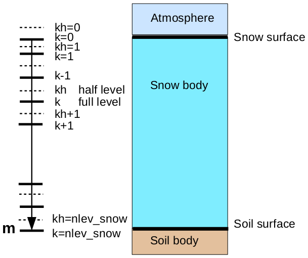
Figure 3 Scheme of the finite-difference representation of the space coordinate in the snow layer.

6 Snow scheme

The processes of formation, transformation, and melting of snow above the soil surface are very important as they are associated with water phase changes, i.e. with a powerful energy source or sink, and with an important thermal insolating layer between the atmosphere and the soil. In this work, an original multilayer scheme for the evolution of snow cover is proposed.

As shown in Sect. 2, from the point of view of thermodynamic processes, the snow layer may either cover the entire surface or be completely absent. However, a concept of minimal snow thickness is introduced above which the snow can be considered a separate layer in terms of heat transport and phase changes. If the snow layer thickness is smaller than this minimum value, the snow is considered an additional component of the soil surface (Sect. 5). At the same time, when considering water balance, i.e. processes related to atmospheric precipitation and water vapour condensation and sublimation, the snow layer thickness can be arbitrarily small; i.e. there is no minimum layer thickness.

The snow layer can be approximated as a porous ice mass which can contain water in the liquid phase formed either by melting of the mass itself or because of incoming liquid precipitation. This liquid water, as soon as it appears, flows into the deepest layers of snow or in the soil. On the snow surface, sublimation from the solid ice phase takes place.

The proposed model uses the snow mass per unit area (kg m⁻²) as a vertical coordinate in the snow layer instead of the more common geometric length, so the term layer thickness here refers to the amount of snow mass associated with a layer rather than its geometrical thickness. The vertical discretization includes full and half levels, the topmost full level has the index 0, the level index increases with depth, and each half level is situated above the full level with the same index (Fig. 3). With the use of this vertical coordinate, each layer, except the topmost one, has the same, constant standard thickness. An increase or decrease in total snow mass first changes the thickness of the top layer. If this thickness reaches or exceeds the standard thickness or becomes smaller than a minimum value, a layer is added or removed respectively. In these cases, the values of snow temperature and melted water content are recomputed considering the newly appeared or disappeared level so that, throughout the snow column, the total snow entropy, the liquid water content, and other diagnostic characteristics such as snow age and density are preserved. However, the number of vertical snow levels cannot exceed a given value. When the snow cover thickness is such that this number of vertical levels is not enough, the standard layer thickness is increased (doubled) for that point, and all the prognostic and diagnostic quantities are recomputed on the new set of levels with conservation of the vertical integral values. The opposite happens when, in the case of snow mass reduction, the number of levels becomes too small; in that case, the standard thickness is reduced (halved) down to the initial standard thickness. In this way, the numerical scheme allows for representing a snow cover of arbitrary thickness, following its thickening or thinning, while keeping the number of layers between given limits.

6.1 Dynamics and balance of snow mass

The dynamics of the snow layer mass is determined by the variations of the two components of the snow layer: solid and liquid. The variations of the liquid component take place in the presence of liquid precipitation falling and condensation of water vapour at the top snow level and, in the case of snow melting, in the whole layer; in this case, liquid water flows into the lower layers or into the soil. The general balance of snow mass is determined by the sum of the water fluxes (in all the phases) at the top and bottom layers.

The water mass flux at the top layer is described in Sect. 2 – see Eq. 38 (${\mathrm{\Phi }}_{\text{v snow}}^{\mathrm{turb}}$), Eqs. 41 and 43 (${\mathrm{\Phi }}_{\text{w snow}}^{\mathrm{liq}}$), Eq. 44 (${\mathrm{\Phi }}_{\text{w snow}}^{\mathrm{ice}}$). At the bottom layer, the water mass flux is determined by the liquid water flux from the layer above. The process of water draining along the snow profile is described in the following way: all the liquid water that at the beginning of the time step is found at level k is found at level k+1 at the end of the step; this hypothesis is acceptable since empirical data show that even a very small liquid water draining speed is always higher than the values resulting from this hypothesis. The thickness of the snow layers is on the order of centimetres, and the time step is on the order of a minute; thus, all the water can drain through a layer of any reasonable thickness in a few seconds even with a very low hydraulic conductivity value on the order of 10⁻⁴ m s⁻². The liquid water flux at a half snow layer is thus

$$\begin{array}{}\text{(72)}& {\mathrm{\Phi }}_{mkh}={\displaystyle \frac{m_{k-\mathrm{1}}\cdot \left(\mathrm{1}-f_{\mathrm{ice}k-\mathrm{1}}^{\mathrm{snow}}\right)}{\mathrm{\Delta }t}},\end{array}$$

where Φ_m kh is the flux of liquid water at level kh (kg m⁻² s⁻¹), m_k−1 is the specific (total) snow mass at level k−1 (kg m⁻²), and $f_{\mathrm{ice}k-\mathrm{1}}^{\mathrm{snow}}$ is the fraction of ice phase in the total snow mass at level k−1.

The water flux at the lowest snow half level is the water flux at the soil surface (see Sect. 3).

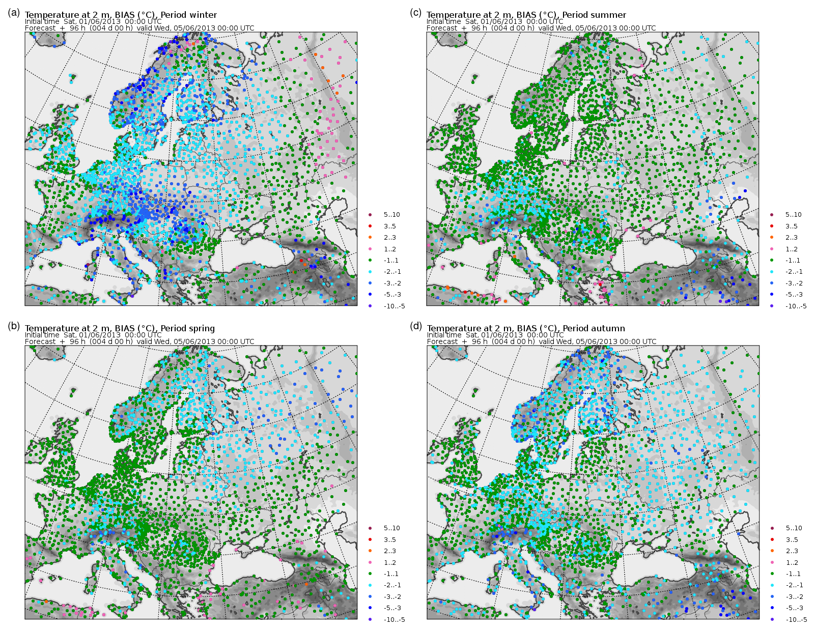
Figure 4 Seasonally averaged bias of temperature at 2 m above surface at observation points: (a) winter, (b) spring, (c) summer, and (d) autumn.

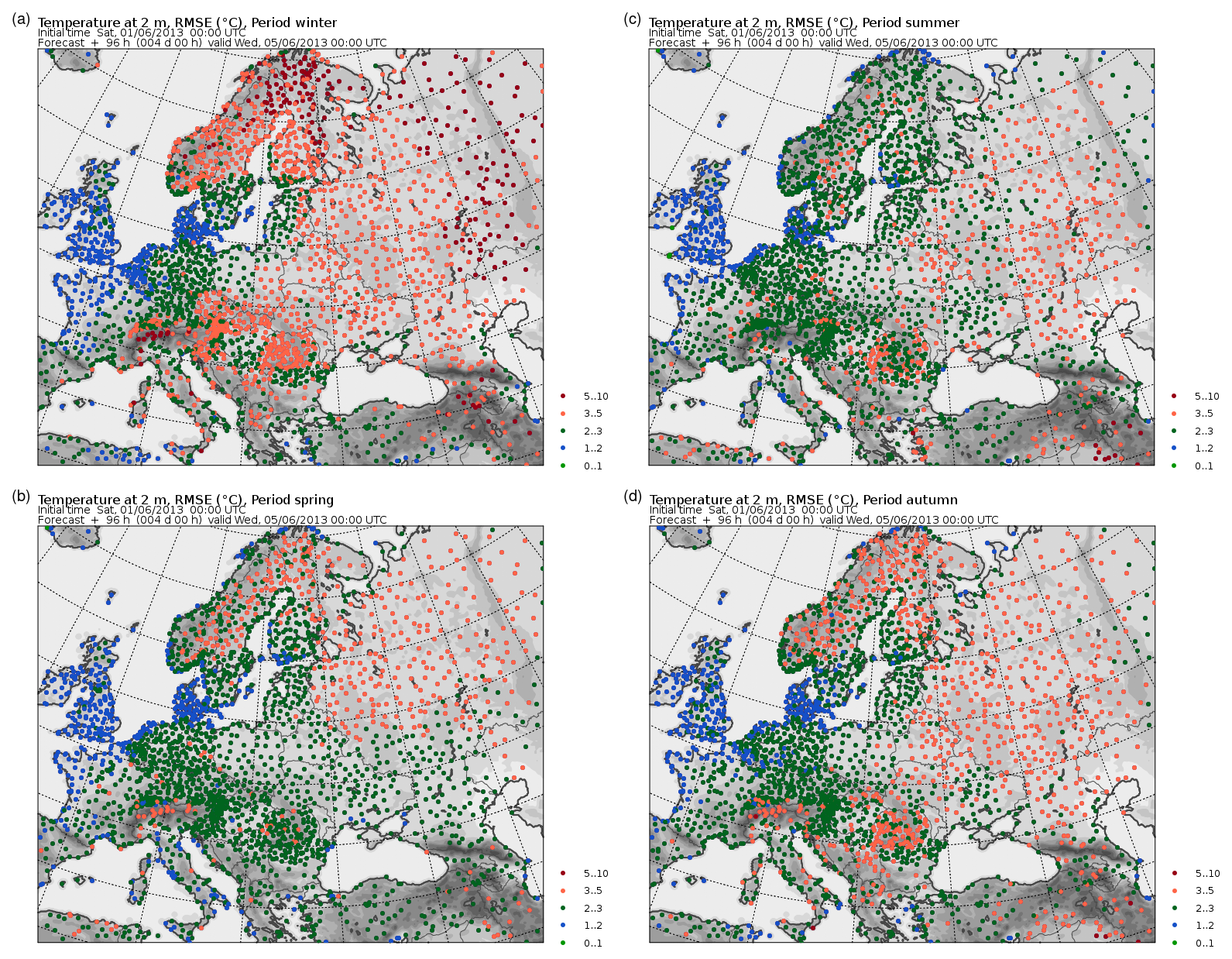
Figure 5 Seasonally averaged RMSE of temperature at 2 m above surface at observation points: (a) winter, (b) spring, (c) summer, and (d) autumn.

6.2 Processes of heat conduction and water phase transition in the snow

As in the soil scheme, the main equation describing the thermodynamic state of the snow is the equation of entropy transport and conservation (see Sect. 5). In the case of snow, for solving the entropy prognostic equation, the splitting method is applied: first, the conductive entropy transport term is solved, and then the entropy conservation in the case of phase transition in the snow layer is solved.

Considering the conductive transport, in mass coordinates, the equation has the following aspect:

$$\begin{array}{}\text{(73)}& {\displaystyle \frac{\partial S_{\mathrm{snow}}^{\mathrm{spec}}}{\partial t}}={\displaystyle \frac{\partial {\mathrm{\Phi }}_{S\mathrm{snow}}}{\partial m}},\end{array}$$

where $S_{\mathrm{snow}}^{\mathrm{spec}}$ is the specific entropy of snow (J K⁻¹ kg⁻¹) and Φ_S snow is the snow entropy flux (J K⁻¹ m⁻² s⁻¹).

By analogy with soil entropy (see Eqs. 60, 61), the total specific entropy of the snow layer, including the solid and liquid phases of water, is defined as

$$\begin{array}{}\text{(74)}& S_{\mathrm{snow}}^{\mathrm{spec}}=C_{\mathrm{snow}}^{\mathrm{\Sigma }}\ln {\displaystyle \frac{T}{T_{\mathrm{0}}}},\end{array}$$

where $C_{\mathrm{snow}}^{\mathrm{\Sigma }}$ is the total specific heat capacity of snow including ice and liquid water (J kg⁻¹ K⁻¹), which can be rewritten, by making use of the concept of the fraction of the solid phase with respect to total mass, in the following way:

$$\begin{array}{}\text{(75)}& C_{\mathrm{snow}}^{\mathrm{\Sigma }}=f_{\mathrm{ice}}^{\mathrm{snow}}{C}_{\mathrm{i}}+\left(\mathrm{1}-f_{\mathrm{ice}}^{\mathrm{snow}}\right)C_{\mathrm{w}}.\end{array}$$

The flux of conductive entropy transport is defined as

$$\begin{array}{}\text{(76)}& {\mathrm{\Phi }}_{S\mathrm{snow}}={\displaystyle \frac{{\mathit{\lambda }}_{\mathrm{snow}}}{C_{\mathrm{snow}}^{\mathrm{\Sigma }}}}\cdot {\mathit{\rho }}_{\mathrm{snow}}^{\mathrm{\Sigma }}\cdot {\displaystyle \frac{\partial S_{\mathrm{snow}}^{\mathrm{spec}}}{\partial m}},\end{array}$$

where λ_snow is the specific heat conductivity of snow (J s⁻¹ m⁻¹ K⁻¹) and ${\mathit{\rho }}_{\mathrm{snow}}^{\mathrm{\Sigma }}$ is the total density of snow including ice and liquid water (kg m⁻³).

In this equation, the density is not the density of the porous medium, but it is a virtual density of the thermodynamically active medium, excluding the pore volume, defined as

$$\begin{array}{}\text{(77)}& {\mathit{\rho }}_{\mathrm{snow}}^{\mathrm{\Sigma }}=f_{\mathrm{ice}}^{\mathrm{snow}}{\mathit{\rho }}_{\mathrm{i}}+\left(\mathrm{1}-f_{\mathrm{ice}}^{\mathrm{snow}}\right){\mathit{\rho }}_{\mathrm{w}}.\end{array}$$

At the same time, a density from the point of view of the porous medium is introduced for the snow in order to define the characteristics of heat conductivity. This density is indicated with the symbol ρ_snow. This quantity is a diagnostic parameter defined at each snow layer, depending on the thickness of the snow layer, the snow age at each layer, and the total period during which the snow at every layer was subject to melting/freezing processes. The following method for determining diagnostic snow density is proposed:

$$\begin{array}{}\text{(78)}& \begin{array}{l}{\mathit{\rho }}_{\mathrm{snow}}=min\left[f_{\mathrm{2}}\cdot f_{\mathrm{3}},{\mathit{\rho }}_{\mathrm{firn}}\right],\\ f_{\mathrm{2}}=max\left\{min\left[{\left(\frac{{\mathit{\tau }}_{\mathrm{snow}}^{\mathrm{melt}}+\mathrm{30}}{\mathrm{395}}\right)}^{\mathrm{0.3}},\mathrm{1}\right]\cdot {\mathit{\rho }}_{\mathrm{firn}},f_{\mathrm{1}}\right\},\\ f_{\mathrm{1}}=max\left\{min\left[{\left(\frac{{\mathit{\tau }}_{\mathrm{snow}}}{\mathrm{365}}\right)}^{\mathrm{0.3}},\mathrm{1}\right]\cdot {\mathit{\rho }}_{\mathrm{snow}}^{\mathrm{old}},{\mathit{\rho }}_{\mathrm{snow}}^{\mathrm{fresh}}\right\},\\ f_{\mathrm{3}}=min\left[\mathrm{1}+\mathrm{0.5}{\left(\frac{m}{\mathrm{100}}\right)}^{\mathrm{0.5}},\mathrm{1.5}\right],\end{array}\end{array}$$

where τ_snow and ${\mathit{\tau }}_{\mathrm{snow}}^{\mathrm{melt}}$ are the total snow age and the total period during which snow was subject to melting (days); ρ_firn, ${\mathit{\rho }}_{\mathrm{snow}}^{\mathrm{fresh}}$, and ${\mathit{\rho }}_{\mathrm{snow}}^{\mathrm{old}}$ are density of firn, fresh snow, and old snow (kg m⁻³); and m is the snow mass in the current layer according to the vertical coordinate used (kg m⁻²). When density is determined, a limitation is applied according to which the density variation cannot exceed 10 % d⁻¹.

The heat conductivity of snow is defined following the study of Jin et al. (1999):

$$\begin{array}{}\text{(79)}& {\mathit{\lambda }}_{\mathrm{snow}}=\mathrm{2.45}\times {\mathrm{10}}^{-\mathrm{6}}\cdot {\mathit{\rho }}_{\mathrm{snow}}^{\mathrm{2}}.\end{array}$$

When Eq. (73) is solved, the snow temperature including the effect of heat conduction is determined, while the solid fraction does not change and is considered known.

We consider now the solution of the second part of the problem, i.e. the conservation of snow entropy in the case of phase transition. The following quantity, equal to the entropy of a particular snow layer including liquid and solid phases, should be preserved:

$$\begin{array}{}\text{(80)}& \begin{array}{rl}& S_{\mathrm{snow}}=\mathrm{\Delta }m\\ & \cdot \left\{f_{\mathrm{ice}}^{\mathrm{snow}}{C}_{\mathrm{i}}\ln {\displaystyle \frac{T}{T_{\mathrm{0}}}}+\left(\mathrm{1}-f_{\mathrm{ice}}^{\mathrm{snow}}\right)\left(C_{\mathrm{w}}\ln {\displaystyle \frac{T}{T_{\mathrm{0}}}}+{\displaystyle \frac{L_{\mathrm{i}}^{\mathrm{w}}}{T_{\mathrm{0}}}}\right)\right\},\end{array}\end{array}$$

where S_snow is the entropy of snow (J K⁻¹ m-2) and Δm is the specific mass of a snow layer (kg m⁻²).

In order to numerically solve Eq. (73), a discretization of the vertical coordinate as shown in Fig. 3 is used together with a time-explicit method of approximation of fluxes and of their derivatives. The following finite-difference prognostic equation is thus obtained:

$$\begin{array}{}\text{(81)}& \begin{array}{rl}& {\displaystyle \frac{C_{\mathrm{snow}k}^{\mathrm{\Sigma }}\ln \frac{T_k^{\ast }}{T_{\mathrm{0}}}-C_{\mathrm{snow}k}^{\mathrm{\Sigma }}\ln \frac{T_k^{\mathrm{0}}}{T_{\mathrm{0}}}}{\mathrm{\Delta }t}}={\mathit{\rho }}_{\mathrm{snow}k}^{\mathrm{\Sigma }}\\ & \cdot {\displaystyle \frac{\begin{array}{c}\frac{{\mathit{\lambda }}_{\mathrm{snow}}^{kh+\mathrm{1}}}{C_{\mathrm{snow}kh+\mathrm{1}}^{\mathrm{\Sigma }}}\frac{C_{\mathrm{snow}k+\mathrm{1}}^{\mathrm{\Sigma }}\ln \frac{T_{k+\mathrm{1}}^{\mathrm{0}}}{T_{\mathrm{0}}}-C_{\mathrm{snow}k}^{\mathrm{\Sigma }}\ln \frac{T_k^{\mathrm{0}}}{T_{\mathrm{0}}}}{m_{k+\mathrm{1}}-m_k}\\ -\frac{{\mathit{\lambda }}_{\mathrm{snow}}^{kh}}{C_{\mathrm{snow}kh}^{\mathrm{\Sigma }}}\frac{C_{\mathrm{snow}k}^{\mathrm{\Sigma }}\ln \frac{T_k^{\mathrm{0}}}{T_{\mathrm{0}}}-C_{\mathrm{snow}k-\mathrm{1}}^{\mathrm{\Sigma }}\ln \frac{T_{k-\mathrm{1}}^{\mathrm{0}}}{T_{\mathrm{0}}}}{m_k-m_{k-\mathrm{1}}}\end{array}}{m_{kh+\mathrm{1}}-m_{kh}}},\end{array}\end{array}$$

where the indices k and kh indicate the values on the full and half vertical levels respectively, the upper indices 0 and * indicate the values of temperature before and after the solution of the conductive heat transport equation respectively. The values of the physical parameters at half levels are computed as the arithmetic mean of the values at the contiguous full levels. In order to compute the overall virtual density (density used in thermodynamics) and heat capacity of snow, the value of the solid fraction of snow layer at the beginning of the time step is used.

Solution of Eq. (81) allows for computing temperature T^∗ after taking into account the conductive heat transfer but without considering the phase transition.

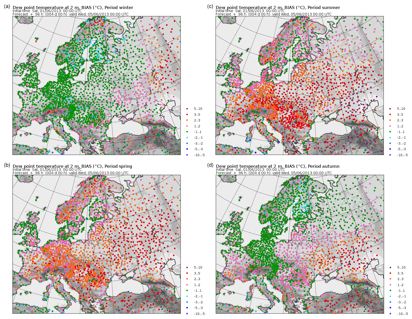
Figure 6 Seasonally averaged bias of dew-point temperature at 2 m above surface at observation points: (a) winter, (b) spring, (c) summer, and (d) autumn.

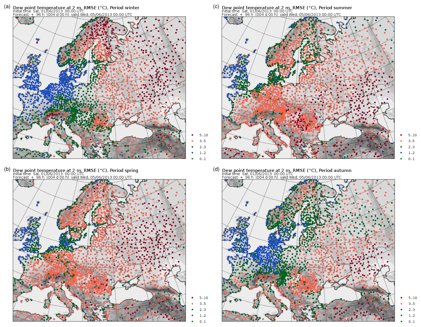
Figure 7 Seasonally averaged RMSE of dew-point temperature at 2 m above surface at observation points: (a) winter, (b) spring, (c) summer, and (d) autumn.

After having solved the first part of the split problem, which provided the value of temperature T^∗, it is possible to define the value of snow entropy, which is considered the definitive value at the end of the time step. For determining entropy, the finite-different discretization of Eq. (80) is used:

$$\begin{array}{}\text{(82)}& \begin{array}{rl}& S_{\mathrm{snow}k}^{\mathrm{\Delta }t}=\\ & \left\{f_{\mathrm{ice}k}^{\mathrm{snow}\mathrm{0}}{C}_{\mathrm{i}}\ln {\displaystyle \frac{T_k^{\ast }}{T_{\mathrm{0}}}}+\left(\mathrm{1}-f_{\mathrm{ice}k}^{\mathrm{soil}\mathrm{0}}\right)\left(C_{\mathrm{w}}\ln {\displaystyle \frac{T_k^{\ast }}{T_{\mathrm{0}}}}+{\displaystyle \frac{L_{\mathrm{i}}^{\mathrm{w}}}{T_{\mathrm{0}}}}\right)\right\}\\ & \cdot \left(m_{kh+\mathrm{1}}-m_{kh}\right),\end{array}\end{array}$$

where $f_{\mathrm{ice}k}^{\mathrm{snow}\mathrm{0}}$ is the fraction of the solid phase at level k before taking into account phase transitions.

Equation (82) includes two unknowns: temperature and fraction of the solid phase. Unlike the case for soil moisture, it is assumed that in the snow layer, the presence of water in the liquid phase ($f_{\mathrm{ice}}^{\mathrm{snow}}<\mathrm{1}$) is possible only at 0 °C (T=T₀). This assumption simplifies the solution: either the initial temperature is T₀, and then Eq. (82) has a single unknown, i.e. fraction of solid phase, or the initial temperature is below zero, and then the only unknown is temperature, which has to be below or equal to 0 °C. The temperature and fraction of the solid phase determined in this way are considered final at the end of the time step.

As remarked in Sect. 5, the solution of the thermodynamic state of the snow layer is performed only when the amount of snow exceeds a given threshold in order to avoid numerical problems. If the snow specific mass is below the given threshold, its thermodynamic state is described by the solution of the entropy equation at the top soil level, whose entropy is augmented by the value of entropy for snow.

The solution of Eq. (82) allows for diagnosing the length of the time interval during which the snow is exposed to melting. The value of this interval is required for computing snow density.

In conclusion, the scheme of snow layer processes defines the overall specific snow mass and its distribution along the vertical levels. Furthermore, it defines at each level the temperature, fraction of the solid phase, snow age, length of melting time interval, and snow density.

7 Verification of the Pochva scheme in the NWP model Bolam in hindcast regime

The Pochva scheme, described above, was developed for use in numerical atmospheric models as a parameterization of heat and water exchange processes at the surface. However, it can be also applied in a column variant using observational data on energy and water fluxes at the surface. Such application allows for studies of soil physical parameters as well as for testing the scheme itself. The results of such testing using observations from the Coordinated Energy And Water Cycle Observation Project (CEOP) Baltic Sea Experiment (BALTEX) are presented in Appendix A.

The Pochva scheme is available as free and open-source software, and it has been implemented in a way that makes it easily adaptable to any atmospheric model. The input data required are atmospheric variables at the lowest level together with fluxes of precipitation, visible and infrared radiation, heat, and humidity (or variables allowing for computing these fluxes). Besides these variables, quantities defining the physical characteristics of soil and vegetation are required. Soil characteristics are allowed to vary along the vertical direction as well. In Pochva, the bottom boundary condition for temperature and soil moisture can be specified through a climatological level, with a horizontally varying depth, depending on the local climatological and hydrological conditions, at which the values of temperature and moisture content are considered constant. The description of the methods used to define the physical parameters of soil and vegetation and the method to define the climatological level may be the subject of a future task. Here, we remark that the spatial variability in soil physical parameters has been defined on the basis of the FAO dataset (FAO – Unesco, 1997), and the vegetation types and the corresponding physical parameters have been defined using the GLC2000 dataset (Joint Research Centre, 2003). Regarding the definition of the climatological levels, these have been set following the analysis of air temperature at 2 m above the surface for the period 1979–2014 from the ECMWF ERA-Interim dataset and the FAO soil type dataset.

In order to test the implementation, the Pochva scheme was included in the NWP (numerical weather prediction) model Bolam (Buzzi et al., 1994, 1998) and in its global variant Globo (Malguzzi et al., 2011). Bolam is a hydrostatic NWP model on a limited area. A numerical experiment in hindcast regime was set up with Bolam; the experiment consisted of a continuous integration of the model over a long period using objective analysis data as boundary conditions during the whole period. As initial and boundary conditions, data of the ECMWF IFS model from the ECMWF operational archive were used. The model domain covered most of European territory. The time extent of the experiment covered the period June 2013–November 2015, with the first 6 months being used to allow the soil layer to reach the thermodynamic equilibrium with the climatological bottom boundary conditions. Consequently, these 6 months were excluded from the subsequent analysis of the results. In this way, the effective period includes 2 full years, from the beginning of December 2013 to the end of November 2015. The length of 2 years was chosen in order to exclude the presence of interannual oscillations and trends in the simulations.

In order to verify the results, data from standard meteorological observations from WMO GTS (World Meteorological Organization Global Telecommunication System) network, retrieved from the ECMWF archive, were used. The main purpose of the numerical experiment was to evaluate the contribution of the Pochva scheme to the numerical modelling results; thus, the variables used in the verification process were the air temperature and the dew-point temperature at 2 m above the surface.

The experiment shows that the main scores, such as the mean error (bias) and root mean square error (RMSE), of near-surface temperature and humidity, stratified on monthly and seasonal intervals do not vary significantly among the 2 simulated years. This suggests that there is no significant trend due to error accumulation in the simulation. In the following, scores averaged over seasonal intervals based on the 2 simulated years are shown.

Figures 4 and 5 show seasonal averages of the temperature bias and RMSE over observation points. As it can be seen from Fig. 4, the bias obtained is relatively low and mostly between −1 and +1 °C. A higher error is noticed in the cold seasons (winter, autumn), when central Europe experiences bias values between −1 and −3 °C (up to −5 °C in mountainous areas), while at the east of the Ural Range, the bias sign is opposite (+1, +2 °C). In the warm seasons, and mainly in summer, a bias of up to +5 °C is noticed in the desert or semi-arid areas of the eastern Mediterranean.

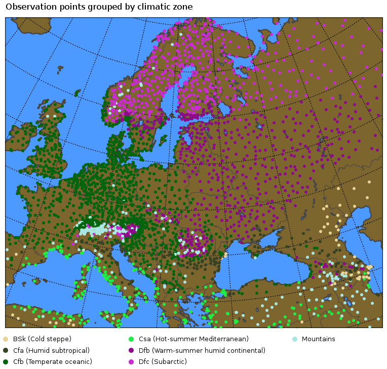
Figure 8 Distribution of observation points by climatic zone according to Köppen–Geiger classification.

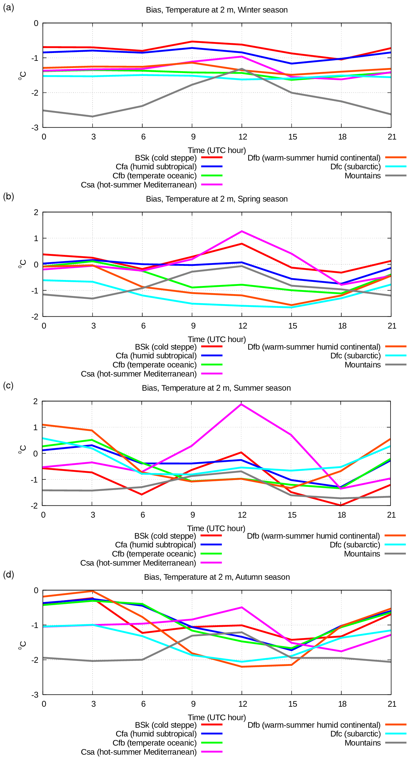
Figure 9 Diurnal cycle of bias of simulated temperature at 2 m above surface for various seasons, i.e. (a) winter, (b) spring, (c) summer, and (d) autumn, in various climatic zones: cold steppe (Bsk, red line), humid subtropical (Cfa, blue line), temperate oceanic (Cfb, green line), hot-summer Mediterranean (Csa, violet line), warm-summer humid continental (Dfb, orange line), subarctic (Dfa, azure line), mountains (grey line).

Figure 10 Same as Fig. 9 but for RMSE of simulated air temperature at 2 m above surface.

The RMSE shown in Fig. 5 also indicates that, in the background of an error with a magnitude of 2–3 °C, the error is higher in the colder seasons, especially in mountain and continental areas, reaching up to 5 °C. In general, coastal areas show a lower RMSE, with values lower than 2 °C, and growing up to 3–5 °C with increasing distance from the sea.

It can be concluded that the overall near-surface atmospheric thermal regime is simulated with enough accuracy. The errors in the cold periods in continental and mountainous areas can be attributed to poor simulation of the snow cover, which strongly influences the near-surface temperature, while high errors in desert areas during the warm periods can be due to either an error in the soil surface temperature or an inaccurate representation of surface turbulent exchange in cases of dry thermal instability.

Figure 6 shows the seasonal dew-point temperature bias at observation points. In the cold seasons the systematic error is in the interval from −1 to +2 °C, while in the warm seasons, the dew-point temperature (and thus air humidity) is overestimated in the continental areas, with a bias growing up to +3 to +5 °C with increasing distance from the sea. Similar conclusions may be drawn from the analysis of the seasonal RMSE, presented in Fig. 7. In the coastal areas all year round and anywhere in the colder seasons, RMSE has low or moderate values of 1–3 °C, while in the continental areas in the warm seasons, it may grow up to 5 °C and more. It can thus be noticed that most of the RMSE is explained by the bias. The overestimation of air humidity in the continental areas during warm seasons is difficult to explain. The absence of a corresponding systematic error for temperature suggests that it is not due to an overestimation of evaporation since, if that were the case, temperature would have been underestimated. It can be assumed that this is due to inaccuracy in the definition of water vapour fluxes or of the humidity profile in the surface layer in the warm season, i.e. in cases of neutral or unstable stratification.

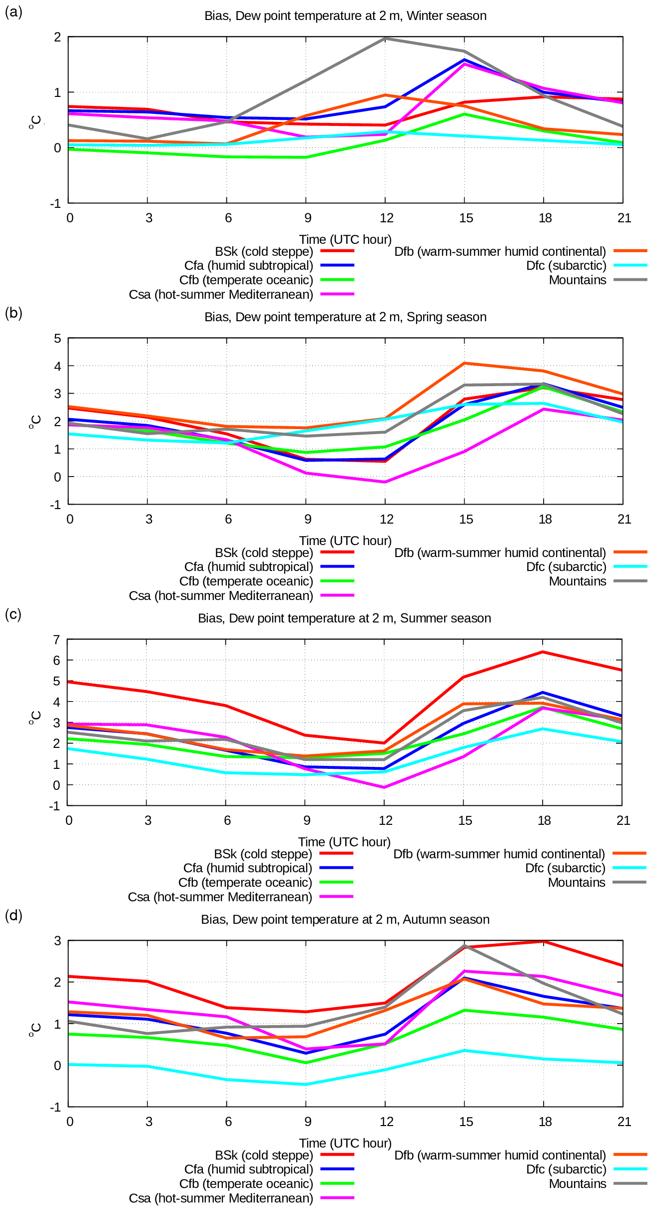
Figure 11 Diurnal cycle of bias of simulated dew-point temperature at 2 m above surface for various seasons, i.e. (a) winter, (b) spring, (c) summer, (d) autumn, in various climatic zones: cold steppe (Bsk, red line), humid subtropical (Cfa, blue line), temperate oceanic (Cfb, green line), hot-summer Mediterranean (Csa, violet line), warm-summer humid continental (Dfb, orange line), subarctic (Dfa, azure line), mountains (grey line).

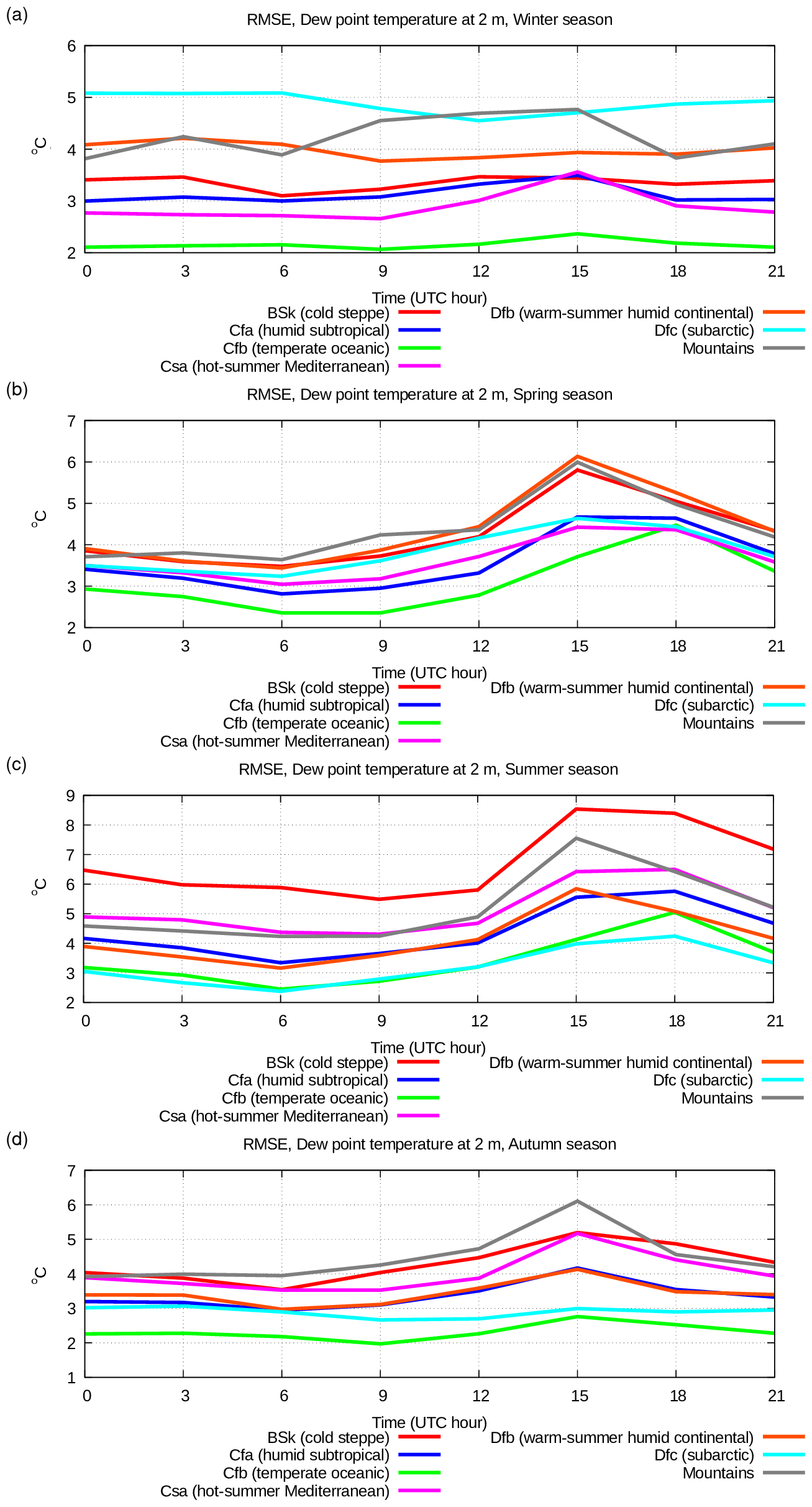
Figure 12 Same as Fig. 11 but for RMSE of simulated dew-point temperature at 2 m above surface.

For a more detailed examination of the errors in near-surface air temperature and humidity from the point of view of the representation of daily cycle, the simulated and observed values for these variables at all the observation times are shown here, averaged over each season and specific geographical areas. Since the model domain covers areas with completely different meteorological and climatological characteristics, the geographical averaging has been carried out considering climatologically uniform areas. For this purpose, a dataset of the Köppen–Geiger climate classification has been used (Rubel and Kottek, 2010). Most of the observation points fall into six climatic areas according to the Köppen–Geiger classification, namely, Bsk (cold steppe), Cfa (humid subtropical), Cfb (temperate oceanic), Csa (hot-summer Mediterranean), Dfb (warm-summer humid continental), and Dfc (subarctic). Furthermore, a separate treatment was adopted for points on mountainous areas, defined as points whose altitude exceeds 1000 m above the mean sea level. Figure 8 shows the distribution of observation points by climatic zone.

For all the observation points falling in each of the seven main climatic zones, the bias and RMSE of temperature and dew-point temperature at 2 m above surface were computed at all the times of the day at which observations are available, namely, 00:00, 03:00, 06:00, 09:00, 12:00, 15:00, 18:00, and 21:00 UTC. Below, the error obtained in the representation of the daily cycle in each climatic zone is examined.

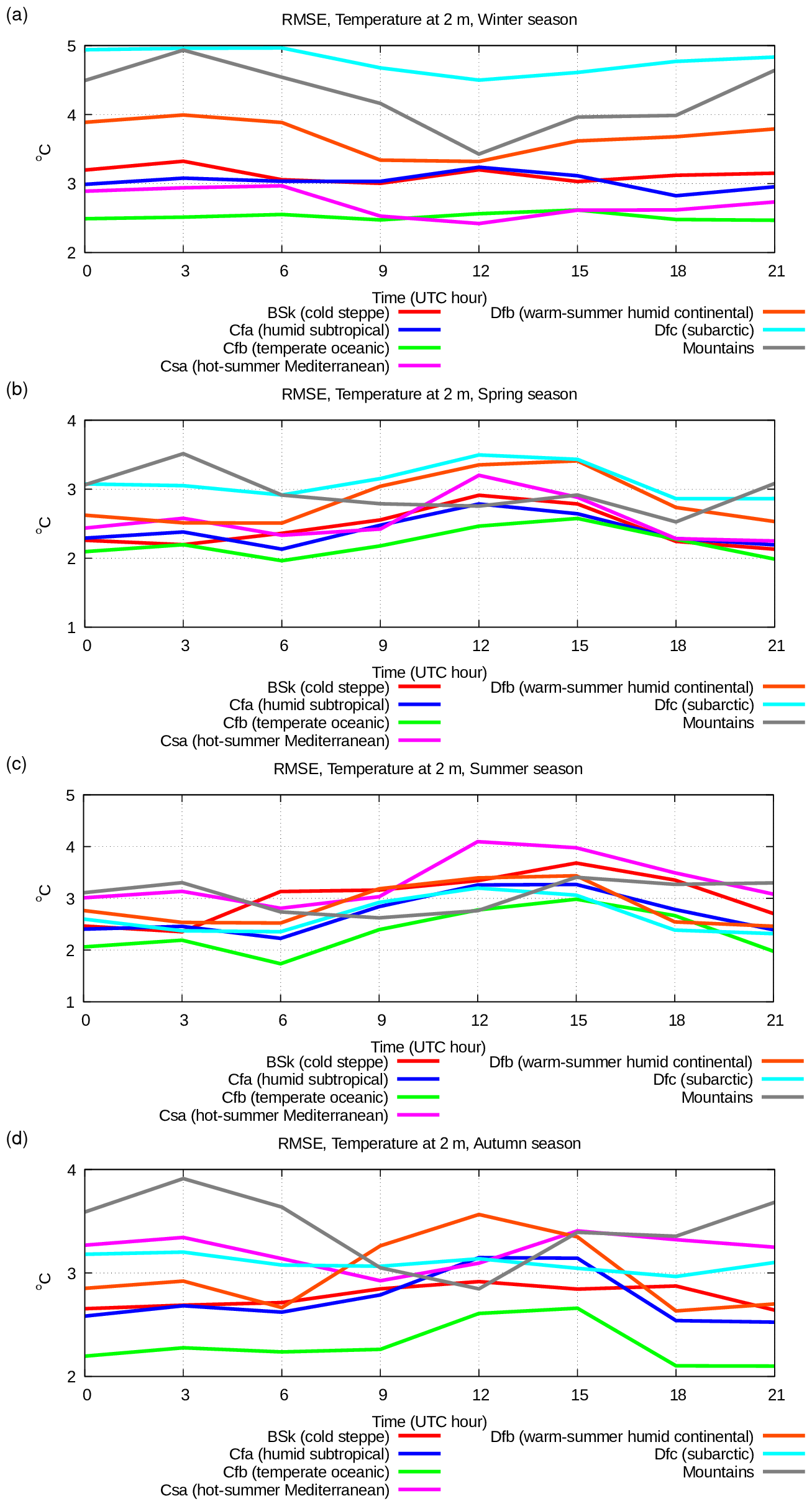
In the winter period (Figs. 9 and 10), the error does not depend on the time of day in all the climatic zones except in the mountainous areas, where the error is higher during the day. In most of the climatic zones, the error is mostly due to bias, which is quite low at −1.3 to 1 °C, while the RMSE is in the range of 1–4 °C. The error is lower in the oceanic climate areas, and it increases in areas with a continental climate. The zone with subarctic climate stands out from this picture since it is characterized by a low bias (−1.5 °C) and high RMSE (4.5–5 °C). At the same time, the mountainous areas, characterized by a similar cold climate, show good scores. This suggests that there are some problems with surface albedo definition in subarctic area and further studies are needed.

During the summer period (Figs. 9 and 10), all the climatic zones are characterized by a relatively low RMSE (2–4 °C), mostly explained by bias, which oscillates between −1.5 and +1 °C. Bias is higher during daytime in the hot-summer Mediterranean climate. This could possibly be due to some problems in the representation of the surface sensible heat flux in the presence of an unstable surface layer or in the surface latent heat flux or due to the insufficient heat capacity of the higher soil layer, which, in turn, could be due to too low values of soil moisture. In areas with mountain and subarctic climate, the score is significantly better in summer than in winter. This is possibly due to deficiencies in the representation of snow cover or of the radiative characteristics of the snow cover itself.

In the spring and autumn periods (Figs. 9 and 10, panels b and d), the scores for 2 m temperature have intermediate values between those for summer and winter. The overall scores are good; the bias ranges between −1.5 and +1.5 °C, while the RMSE is around 2–4 °C. In spring, the error characteristics are closer to the summer ones, while in autumn, they are closer to the winter ones. It is probably the case that the processes of formation and melting of the snow layer in the areas with a stable winter snow cover (warm-summer humid continental, subarctic, and mountains) are simulated more or less correctly since no increase in the error is observed in these transitional seasons.

Concerning the scores for humidity in terms of 2 m dew-point temperature, Figs. 11 and 12 show the daily cycle of the bias and RMSE for this variable.

In the winter period (Figs. 11 and 12, panel a) all the climatic zones are characterized by a low systematic error (0 to +2 °C) and a significant RMSE (2–5 °C) with a very weak daily cycle. In the same way as for temperature, the scores strongly depend on the climatic zone: better scores (RMSE up to 3 °C) are found in the area with an oceanic climate (temperate oceanic, hot-summer Mediterranean, humid subtropical), while the worst scores (RMSE higher than 4 °C) are found in zones with a cold continental climate (warm-summer humid continental, subarctic, mountains). This may be attributed to deficiencies in the definition of latent heat flux or air humidity profile over snow layer, i.e. in cases of stable surface layer.

In the summer period, on the other hand, most of the RMSE (2.5–8.5 °C) is explained by systematic error (0 to +6 °C), which is always positive; i.e. the air humidity is systematically overestimated. In general, the minimum of the daily error occurs at daytime, while it is maximum in the evening and night. This may be due to a suboptimal tuning of the turbulent exchange parameterization in neutral and stable boundary layer conditions. In the areas characterized by oceanic climate or in cold climate areas (temperate oceanic, subarctic), the errors are lower, while in dry areas (cold steppe), they are higher. At the time of day when errors are higher, the overestimation of air humidity is accompanied by the underestimation of air temperature. This may be evidence of deficiencies in the computation of latent heat flux (evaporation).

During the spring and autumn seasons (Figs. 11 and 12, panels b, d), the dew-point temperature scores, similarly to the case of temperature, exhibit intermediate values between those found in winter and summer seasons. In general, the air humidity is almost always overestimated, even more so in the warm season than in the cold season.

The scores presented here show no evidence of systematic deficiencies in the near-surface temperature except during periods characterized by a stable snow cover, when temperature is systematically underestimated, or during summer periods in dry climatic zones, when daytime temperature is overestimated. At the same time, near-surface air humidity is systematically overestimated, especially in summer time, and, in particular, in dry climatic areas in the evening and at night.

As a general conclusion, the results shown by the numerical experiments with the Pochva scheme are definitely convincing.

8 Summary

The model of hydro-thermal processes in vegetated soil and snow cover presented in this work is characterized by a special attention to the soil–water phase transition and by novel approaches to define some soil and snow physical parameters. The proposed model has been validated by a solid verification presented in this work, consisting of a 2-year hindcast experiment. The presented model may be useful for modelling research over polar or cold climate zones, in permafrost evolution studies, in studies and forecast of snow cover, and in studies of the surface layer in stable conditions over cold surfaces. The model is realized using an effective and stable numerical algorithm with a clear, intuitive interface that allows for a simple coupling to an atmospheric model or to observations of energy and water fluxes in the air surface layer and at the surface.

This land model has been included in the Institute of Atmospheric Sciences and Climate (CNR-ISAC) NWP models: Globo (hydrostatic approximation, global domain); Bolam, described above; and Moloch (non-hydrostatic, high space resolution at limited area). The indicated NWP models with Pochva are used from 2018 up to present day for the routine operational weather prediction in CNR-ISAC for the Civil Protection Department of Italy. Forecast products are available at https://www.isac.cnr.it/dinamica/projects/forecasts/ (last access: May 2025), and the results of forecast verification are available at https://www.isac.cnr.it/dinamica/projects/forecast_verif (last access: May 2025).

Appendix A

A test of Pochva scheme in its column version has been performed using observational data of Coordinated Energy and Water Cycle Observation Project (CEOP) Baltic Sea Experiment (BALTEX). The observed data have been used as forcing parameters for Pochva simulations, determining the physical parameters of the soil profile, and defining the initial condition. The observed data have also been used for the verification of simulation results. The observations were carried out at Falkenberg, a site of the German Weather Service Meteorological Observatory. This site is located in grassland fields, in a heterogeneous rural landscape typical of central Europe. The observational data are freely available upon individual request.

Table A1 Physical parameters of the soil at the Lindenberg–Falkenberg observation station adapted from Beyrich (2011c).

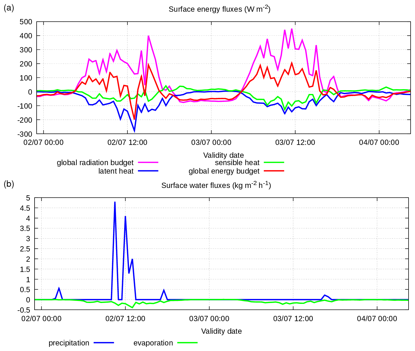
Figure A1 Observation data (BALTEX) in Falkenberg on 2–3 July 2003. Parameters at the surface: (a) solar radiation and heat fluxes (W m⁻²) and (b) precipitation and evaporation rate (kg m⁻² h⁻¹).

To apply the soil scheme offline, the values of the soil physical parameters and the soil temperature and water content profiles must be defined at the beginning of the simulation; top and bottom conditions for the prognostic variables must be defined for each time step during the simulation. A time step of 60 s was used in the simulation. Values of soil physical parameters in Pochva simulations are defined following the values measured at the observation point and presented in Table A1, taken from dataset documentation (Beyrich, 2011c). The initial condition for prognostic variables, soil temperature, and soil water content, can be defined using the measurements at the soil levels. The bottom boundary conditions for prognostic variables can be defined using observation data at the lowest measurement level interpolated in time. The top boundary condition for prognostic variables, surface temperature, surface air humidity, and surface soil water content can be defined by heat and water mass fluxes at the surface: radiation flux (global net and visible incident), sensible and latent heat flux, precipitation flux, and water vapour flux. The indicated surface fluxes have to be defined using the measurement data at the surface and in the air surface layer.

The observation dataset contains measurement for the following variables: soil temperature at 0.05, 0.10, 0.15, 0.20, 0.30, 0.45, 0.50, 0.60, 0.90, 1.00, 1.20, and 1.50 m depth; specific volumetric soil water content at 0.08, 0.15, 0.30, 0.45, 0.60, and 0.90 m depth; pressure and temperature at the surface, air temperature, and air humidity at 2.4 m above the surface; wind at 10 m above the surface; pressure, air temperature, air humidity, and wind at 40 and 80 m above the surface; downward and upward short-wave and long-wave solar radiation at the surface; precipitation at the surface; and sensible and latent heat flux 2.4 m above the surface. These data are presented in Beyrich (2011a, c).

To avoid vertical interpolation of simulated data when comparing with observations, the Pochva simulation uses the same soil levels where soil temperature and water content measurements are available, namely, 0.02, 0.05, 0.08, 0.10, 0.15, 0.20, 0.30, 0.45, 0.50, 0.60, 0.90, 1.00, 1.20, and 1.50 m depth. The bottom condition for soil temperature is defined at 1.5 m depth using the bottom temperature measurement level, whereas the bottom condition for soil water content is defined at 0.9 m depth using the bottom measurement level for this parameter. Since the lower boundaries for the prognostic variables in these simulations are not deep, a few days of simulation may be sufficient to reach the numerical thermodynamic equilibrium regime.

The indicated measurement list contains all the parameters required for defining the top soil boundary condition. These parameters are also named atmospheric forcing parameters. They are the following: sensible and latent heat flux at 2.4 m above the surface, downward and upward short-wave and long-wave radiation at the surface, and precipitation at the surface (water vapour flux at the surface cat be estimated using observed latent heat flux).

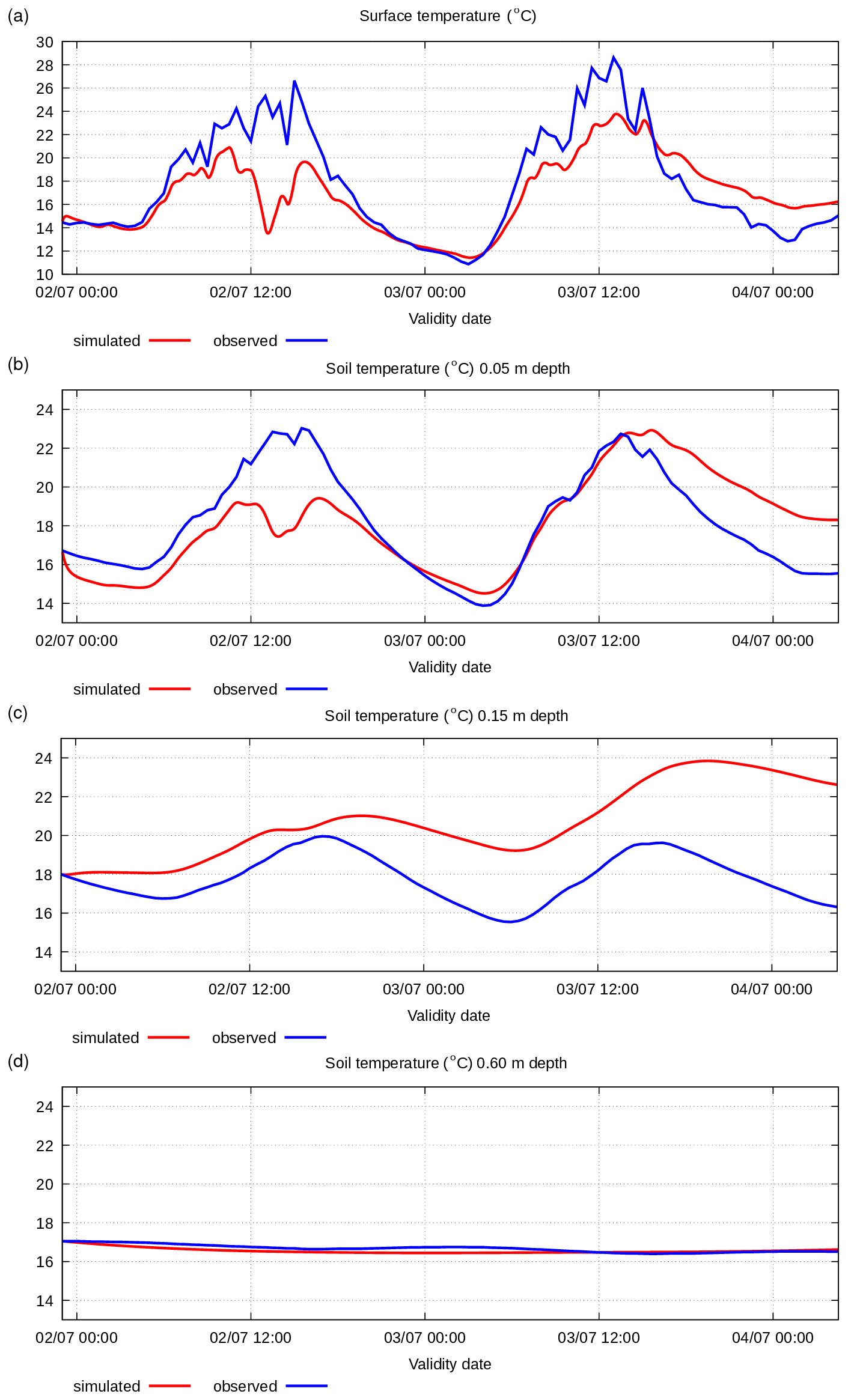
Figure A2 Simulated and observed 2–3 July 2003 soil temperature (°C) at the surface and at various depths: (a) surface, (b) −0.05 m, (c) −0.15 m, and (d) −0.60 m.

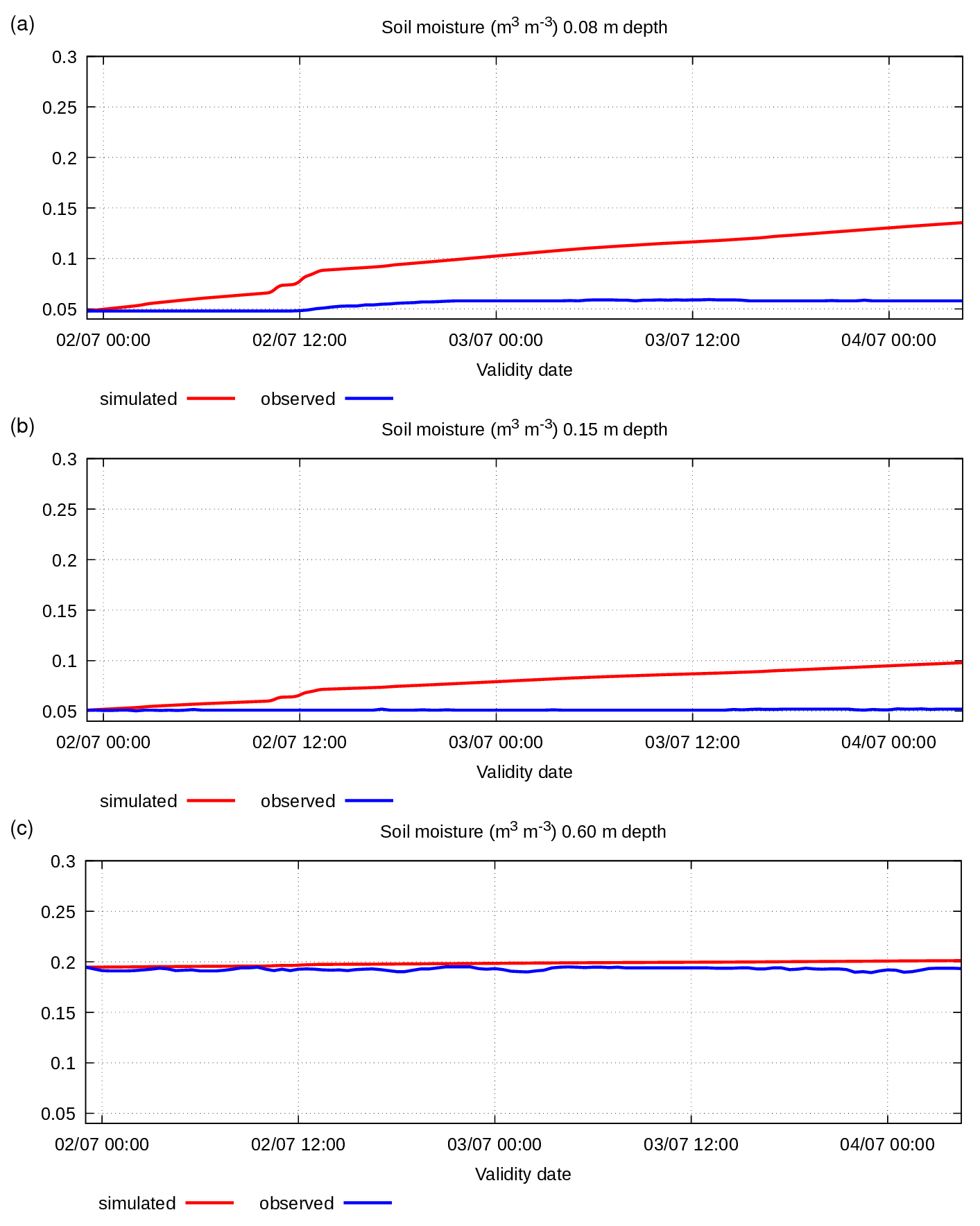
Figure A3 Simulated and observed 2–3 July 2003 soil specific volumetric water content (m³ m⁻³) at various depths: (a) −0.08 m, (b) −0.15 m, and (c) −0.60 m.

The observation datasets contain the data for the period from 1 January 2002–31 December 2009. All observed data have a time resolution equal to 30 min. The author has developed a program that reads data from the database for various parameters, identifies the times at which data for all the atmospheric forcing parameters are available, and produces a list of the times found. Another program finds periods without gaps in the obtained list. A third program searches in the database the measurements for all required forcing parameters within the periods of continuous measurements, interpolates these data in time with the step specified for the model simulation (60 s), and prepares all necessary data for the Pochva simulation.

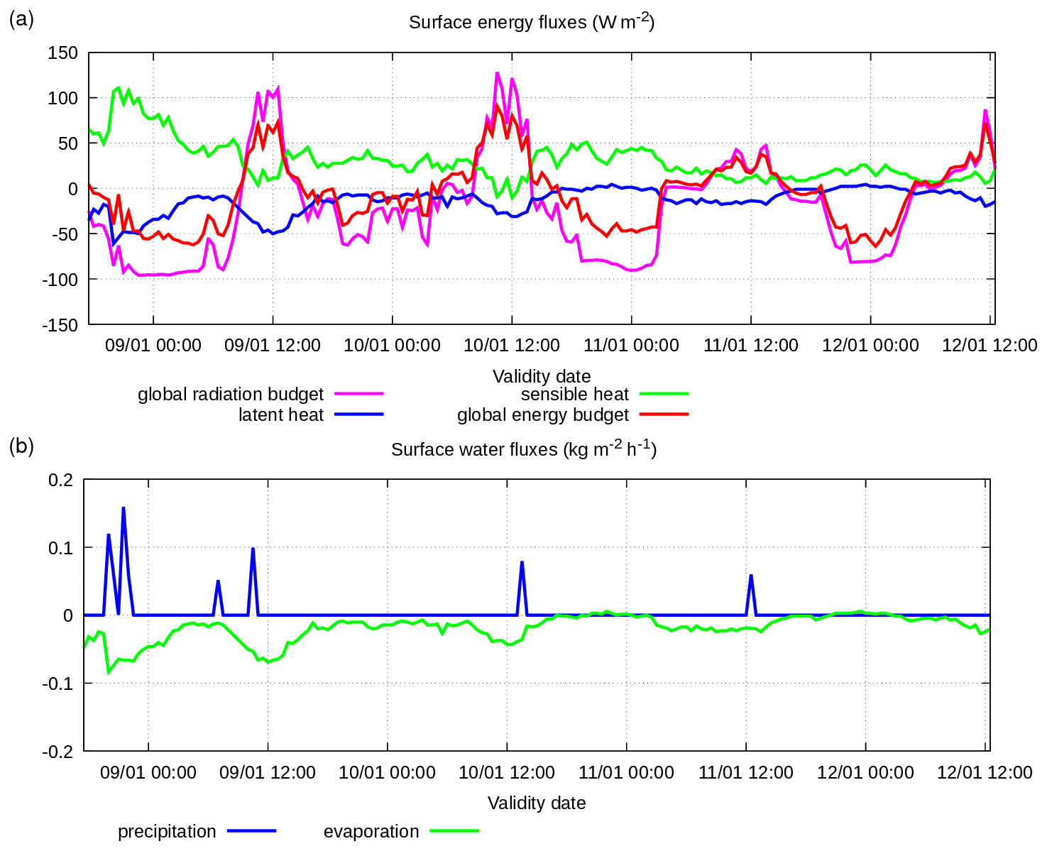
Figure A4 Observation data (BALTEX) in Falkenberg 8–12 January 2005, parameters at the surface: (a) solar radiation and heat fluxes (W m⁻²) and (b) precipitation and evaporation rate (kg m⁻² h⁻¹).

Unfortunately, this search revealed very frequent gaps in the measurements of surface heat fluxes. A search for periods with gaps of no more than 2 h for all the required forcing parameters resulted in 90 periods, the longest of which had a length of 4 d. However, if heat fluxes are excluded from the search of continuous measurement periods, then a very long period of 913 d is found. Therefore, the author decided to perform two types of simulations: one exclusively with the Pochva model using all atmospheric forcing parameters from measurements, the other with the Pochva model coupled with a model of air surface layer processes, which simulates surface heat fluxes using measurements of wind, pressure, air temperature, and air humidity at a height of 40 m above ground level and at the surface.

The author selected two periods for the first type of Pochva simulations, one in summer and one in winter. The initial conditions are defined using the observational data at the date and time of the simulation start. The simulation results and their comparison with the observational data are presented below.

The summer verification period is from 1 July 2003 at 23:00–4 July 2003 at 04:30 (53.5 h). Input data on energy fluxes at the surface and water mass fluxes are shown in Fig. A1.

These July days are characterized by intensive net radiation flux accompanied by moderate sensible and latent heat fluxes; the latent heat flux is significant only after light rain on the first day.

The simulated soil temperature and moisture data are shown in Figs. A2 and A3 together with observed data at the same depth levels.

Figures A2 and A3 show that the simulated soil parameters at the different levels are out of numerical equilibrium. Despite this fact, the simulated parameter values are close to the observed values. The soil temperature simulated at various levels shows a correct daily cycle, especially at the surface and at the top soil levels, which are important for atmospheric model parameterization. Moreover, the observation data show some odd characteristics: light rain was observed on 2 July at 12:30 (Fig. A1b) accompanied by a sharp decrease in solar incoming radiation flux and an increase in the outgoing latent heat flux, thus determining a strongly negative energy budget at the surface. This phenomenon is simulated by Pochva; the simulated surface and soil top temperature evidently drop at this time, while, on the other hand, the observed surface and soil top temperature do not reflect this phenomenon. Furthermore, the observed soil moisture at different levels remains unchanged despite the presence of the significant vertical gradient of soil moisture, rain, and evaporation in the observation data.

The winter verification period is from 8 January 2005 at 17:30–12 January 2005 at 12:30 (91 h). Input data on energy fluxes at the surface and water mass fluxes are shown in Fig. A4.

This January period is characterized by an intensive net radiation flux during the first and second day, with significant daytime heating and night-time cooling, accompanied by weak sensible and latent heat fluxes except for the first night, when a significant sensible heat flux is observed; the latent heat flux is significant only after light rain on the first day. Some episodes of very light precipitation occur. The evaporation flux has small values.

The simulated soil and moisture data at same depth levels are presented in Figs. A5 and A6 together with observed data.

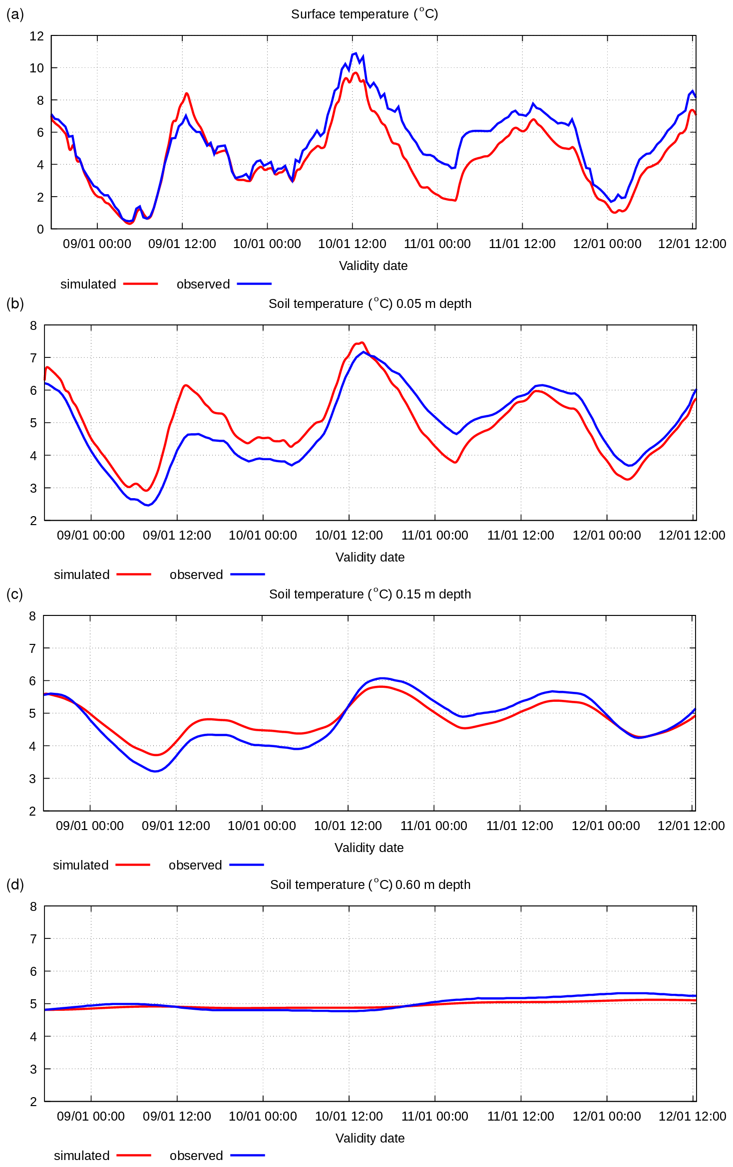
Figure A5 Simulated and observed 8–12 January 2005 soil temperature (°C) at the surface and various depths: (a) surface, (b) −0.05 m, (c) −0.15 m, and (d) −0.60 m.

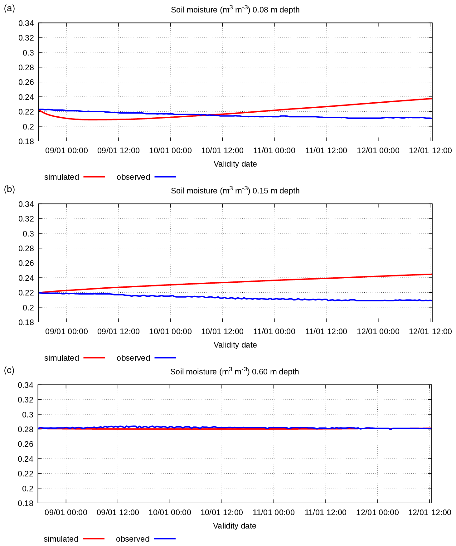
Figure A6 Simulated and observed 8–12 January 2005 soil specific volumetric water content (m³ m⁻³) at various depths: (a) −0.08 m, (b) −0.15 m, and (c) −0.60 m.

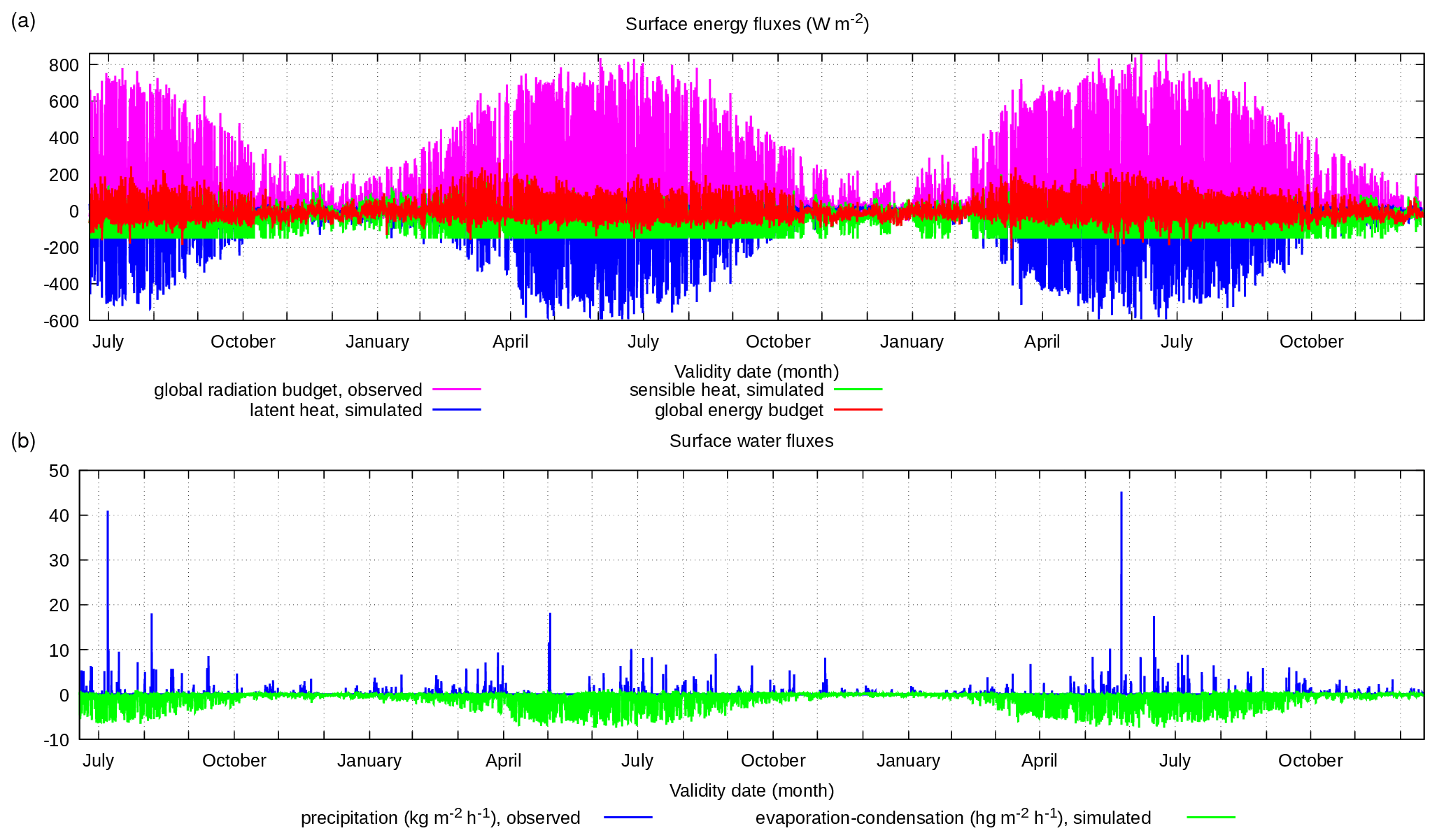
Figure A7 Simulation and observation data for the period 3 July 2007–31 December 2009, parameters at the surface: (a) observed solar radiation (W m⁻²) observed and simulated heat fluxes (W m⁻²) and (b) observed precipitation rate (kg m⁻² h⁻¹) and simulated evaporation rate (hg m⁻² h⁻¹).

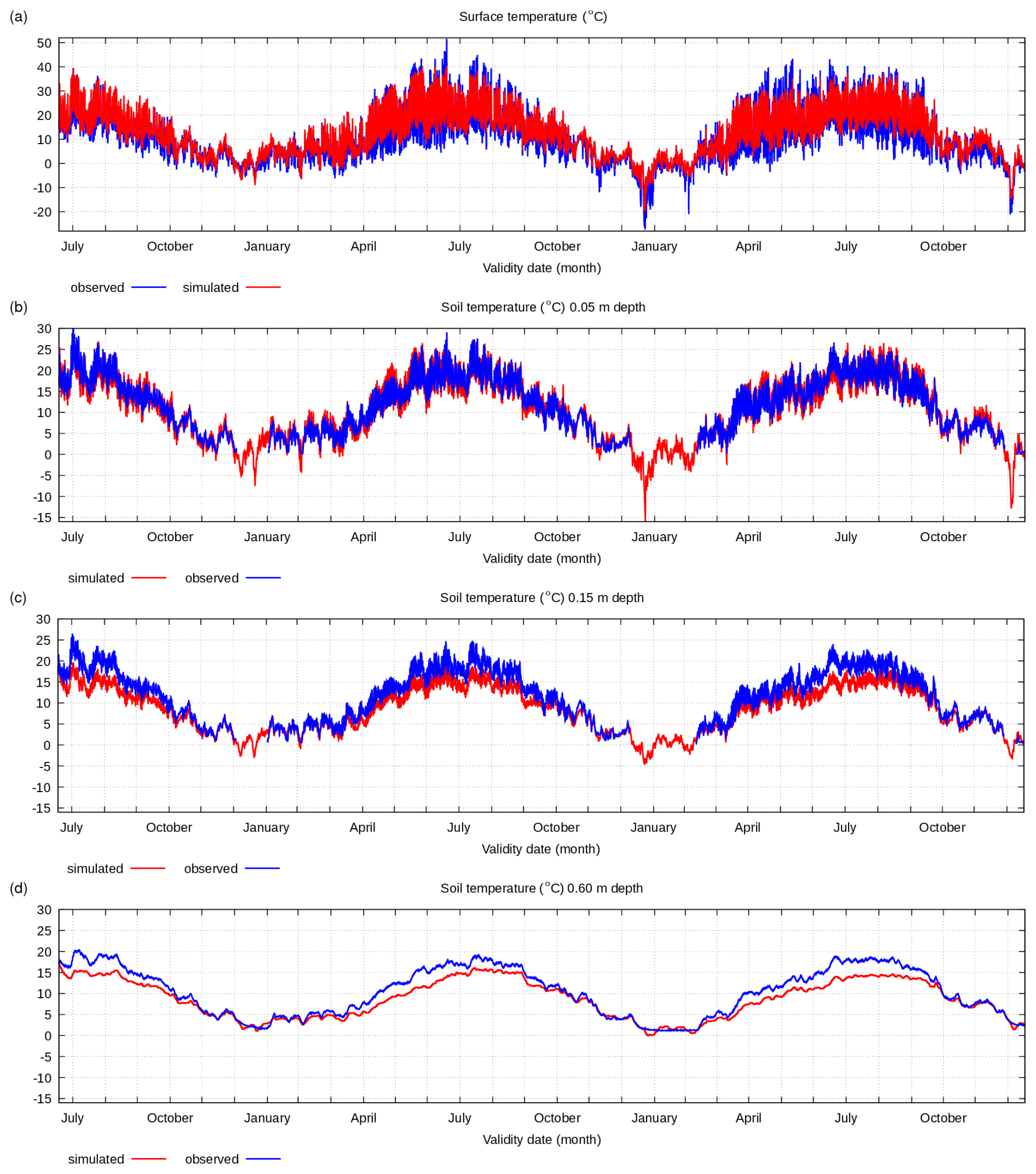
Figure A8 Simulated and observed soil temperature (°C) at the surface and at various depths: (a) surface, (b) −0.05 m, (c) −0.15 m, and (d) −0.60 m for the period from 3 July 2007–31 December 2009.

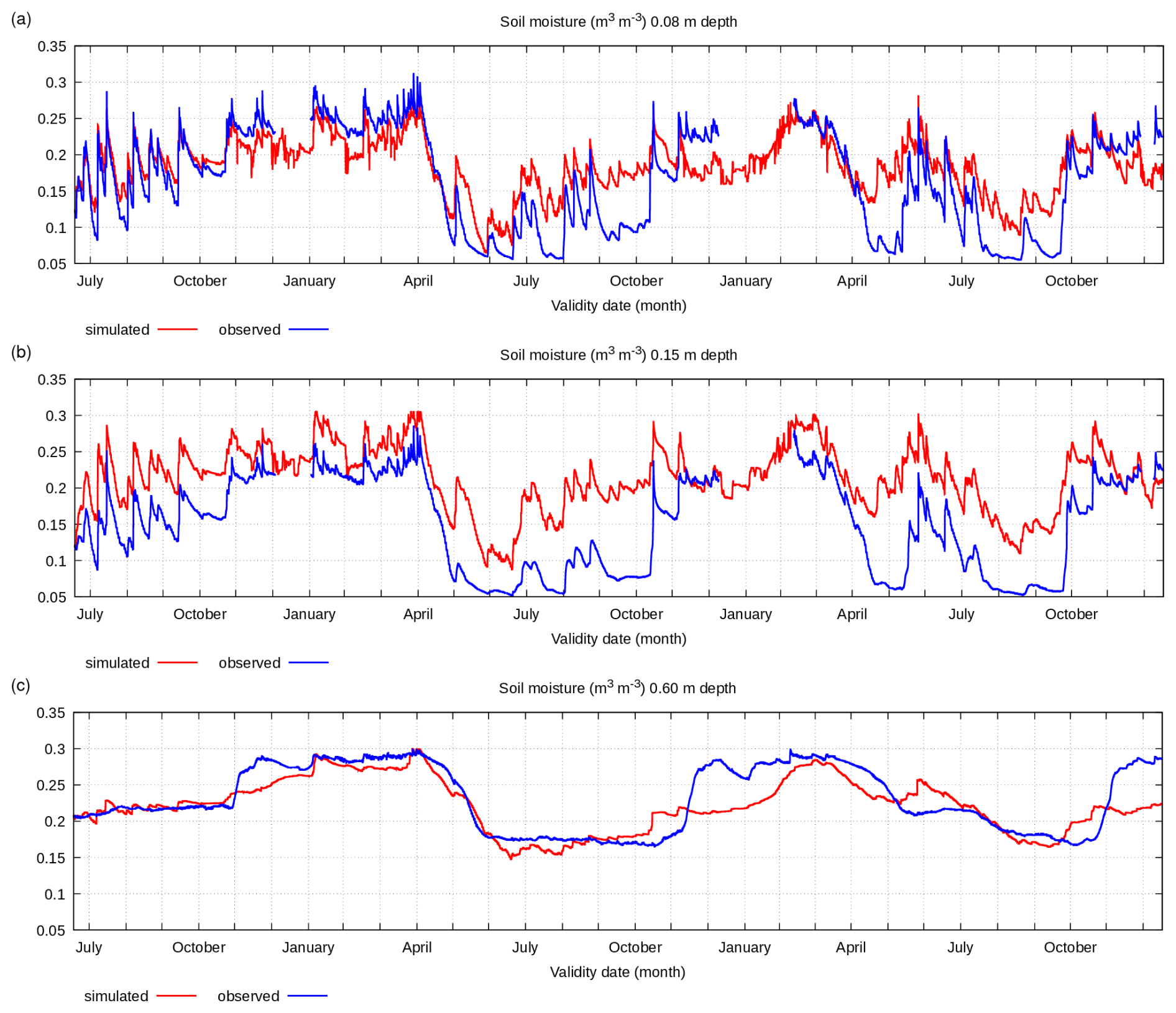
Figure A9 Simulated and observed soil specific volumetric water content (m³ m⁻³) at various depths: (a) −0.08 m, (b) −0.15 m, and (c) −0.60 m for the period from 3 July 2007–31 December 2009.

In this winter case, the initial condition for the soil temperature has a very small vertical gradient. For this reason, the simulated results do not show numerical imbalance. The simulated soil temperature is very close to observed values. At the same time, the initial condition for soil moisture has a significant vertical gradient following observed data. Thus, the simulated soil moisture has the characteristics of numerical disequilibrium similarly to the summer case. However, in this case, the observed moisture has an odd behaviour; it remains almost constant at all vertical levels. The observed soil moisture data indicate that water conductivity is close to zero, but it does not correspond to the conductivity value declared for the observation point (see Table A1). There are probably some measurement inaccuracies.

To summarize, it can be said that the Pochva scheme is able to simulate the soil temperature and moisture correctly enough. The observed values of soil physical parameters, forcing scheme parameters, and initial condition parameters have been used in Pochva simulations with no manipulation, and simulations show results close to observation data.

The second type of Pochva simulation has been performed for the period from 3 July 2007 at 03:00–31 December 2009 at 23:30 (912.85 d), which amounts to almost 3 years. The sensible heat, latent heat, and water vapour fluxes at the surface have not been taken from measurements but simulated by an air surface layer process model based on the Monin–Obukhov similarity theory (Monin and Obukhov, 1955) using wind, air temperature, and air humidity observations at 40 m above the surface and at the surface (Beyrich, 2011b). The simulation results and their comparison with the observation data are presented below.

Input data on energy fluxes at the surface and water mass fluxes are shown in Fig. A7, and the simulated soil temperature and moisture data at same depth levels are shown in Figs. A8 and A9 together with observed data.

Figures A7–A9 show a well-defined seasonal cycle of the surface and soil parameters. Periods with very hot and very cold weather, as well as periods with precipitation, are present in the observed data. As it can be seen in Figs. A8 and A9, unfortunately, at temperatures below 0 °C, the soil temperature and soil water content sensors were not operational during the two winters. However, the surface temperature sensor was in operation during the whole simulation period.

Figures A8 and A9 show that the simulated values for various parameters are close to the observed values. The surface temperature is very close to the observed values (Fig. A8a); this means that Pochva and the air surface layer schemes approximate the energy flux surface equilibrium very well. This is very important because the main task of the Pochva scheme is to correctly simulate the thermal state of the surface for use in a numerical atmosphere model. The simulation of the soil temperature in the middle levels has some problems with underestimation (by 3–5 °C) in the summer months (Fig. A8b, c); this error is also noticeable in the deep layer (Fig. A8d) but less pronounced (2–3 °C). During winter months, when the surface temperature is mostly between 0 and −20 °C, the simulation of soil temperature is correct at all soil levels. The soil water content in the upper layer is mostly correctly simulated (Fig. A9a), except for August 2008 and 2009 and October 2008 and 2009, when soil moisture at 8 cm depth was overestimated. At the same time, the soil water content in the deeper layer was simulated correctly (Fig. A9c).

In summary, it can be noted that the Pochva scheme correctly simulates the temperature and water content of the soil in the upper and lower soil layers in all seasons but in the middle layer only in the cold season, while in the warm season, it underestimates the temperature of this layer and overestimates the water content.