NMH-CS 3.0: a C# programming language and Windows-system-based ecohydrological model derived from Noah-MP

The community Noah with multi-parameterization options (Noah-MP) land surface model (LSM) is widely used in studies ranging from uncoupled land surface hydrometeorology and ecohydrology to coupled weather and climate predictions. In this study, we developed NMH-CS 3.0, a hydrological model written in C# (pronounced C sharp). NMH-CS 3.0 is a new model developed by faithfully translating Noah-MP, written in Fortran, from the uncoupled WRF-Hydro 3.0, and it is coupled with a river routing model. NMH-CS has the capacity to be executed on Windows systems, utilizing the multi-core CPUs commonly available in today's personal computers. The code of NMH-CS has been tested to ensure that it produces a high degree of consistency with the output of the original WRF-Hydro. High-resolution (6 km) simulations were conducted and assessed over a grid domain covering the entire Yellow River basin and most of northern China. The spatial maps and temporal variations in many state variables simulated by NMH-CS 3.0 and WRF-Hydro/Noah-MP demonstrate highly consistent results, occasionally with minor discrepancies. The river discharge for the Yellow River simulated by the new model with various scheme combinations of six parameterizations exhibits general agreement with the natural river discharge at the Lanzhou station. NMH-CS can be regarded as a reliable replica of Noah-MP in WRF-Hydro 3.0, but it can leverage the modern, powerful, and user-friendly features brought by the C# language to significantly improve the efficiency of the model's users and developers.

1 Introduction

In contemporary hydrological prediction and flood warning applications, the effectiveness of hydrological models hinges on their ability to delineate intricate energy and water processes on the land surface, surpassing the capabilities of traditional rainfall–runoff models. To address this demand, certain land surface models (LSMs) utilized by atmospheric science communities have been bolstered by hydrological simulation features, as observed in WRF-Hydro (Lin et al., 2018), or conventional rainfall–runoff models have been enriched with more comprehensive descriptions of land surface processes, exemplified by the VIC model (Liang et al., 1994).

The Noah land surface model with multi-parameterizations (Noah-MP) (Niu et al., 2011; Yang et al., 2011) stands out as a robust tool for studying global water issues, serving as the foundation for models like WRF-Hydro, which incorporates Noah-MP (Gochis, 2020). However, the code for Noah-MP and WRF-Hydro is written in Fortran, a “legacy” language, posing challenges for code analysis and editing, unlike more modern languages such as C# (pronounced C sharp), because Fortran lacks the intelligent, efficient programming tools that are now common for C#. This limitation makes it arduous for users unfamiliar with Fortran to efficiently comprehend and modify the code. Additionally, Noah-MP and WRF-Hydro necessitate a UNIX-like operating system, causing inconvenience for users and developers relying on Windows systems. Therefore, there is a compelling need to code Noah-MP in a contemporary modern programming language and gain wider accessibility to the Noah-MP model.

We designed NMH-CS 3.0, a Noah-MP-based hydrological model coded using the C# programming language. This model was crafted by creating a framework and accurately translating the original Noah-MP LSM code from WRF-Hydro 3.0 and coupling it with a Muskingum-method-based river routing model (Liu et al., 2023). C#, recognized for its modern and object-oriented approach, is widely used for software development across various platforms, particularly on the Windows operating system. According to the TIOBE Programming Community Index (https://www.tiobe.com/, last access: 16 October 2024) for October 2024, C# ranks fifth among major programming languages with a user base of 5.6 %, while Fortran ranks ninth with only 1.8 % of users.

NMH-CS provides several advantages over the original WRF-Hydro/Noah-MP. Unlike the original version, which requires compiling for each computer and primarily depends on UNIX-like systems, NMH-CS can seamlessly run on Windows systems that support the Microsoft .NET Framework. The executable files, once compiled, can be easily packaged and distributed to other Windows machines and offers greater convenience for users who are less familiar with UNIX-like operations. The utilization of the C# language facilitates advanced software tools for visualizing and analyzing the model's code, enhancing the convenience for users to read, modify, and debug the code. This is appealing to model developers who are proficient in the C# language and object-oriented programming. The design of NMH-CS aligns with the input datasets and configurations specified in the “namelist” file, ensuring high compatibility with WRF-Hydro 3.0. Leveraging the parallel computing capabilities of C#, both the translated Noah-MP LSM simulation and the river routing simulation within NMH-CS support parallel execution on common personal computers.

2 The Noah-MP LSM

Noah-MP is a robust model renowned for its capability to represent diverse physical processes. Since its initial introduction (Niu et al., 2011; Yang et al., 2011), Noah-MP has been widely used. For example, Noah-MP has been coupled to WRF-Hydro as a major module and can be seamlessly integrated into the Weather Research and Forecasting (WRF) model (Gochis, 2020). Furthermore, the offline WRF-Hydro model plays a pivotal role in the National Water Model, contributing to the simulation of floods and river flows across the United States (Bales, 2019; Francesca et al., 2020; Karki et al., 2021). Noah-MP's versatility extends to applications such as streamflow prediction (Lin et al., 2018) and the estimation of evapotranspiration, surface temperature, carbon fluxes, heat fluxes, and soil moisture, as demonstrated in many studies (Chang et al., 2020; Gao et al., 2015; Li et al., 2022; Ma et al., 2017; Yang et al., 2021). Noah-MP is supported by several different modeling frameworks to facilitate coupling it to various Earth system framework models including HRLDAS (Chen et al., 2007), LIS (Kumar et al., 2006), and WRF-Hydro (Gochis, 2020). This makes Noah-MP a powerful research and forecasting tool within the hydrology community.

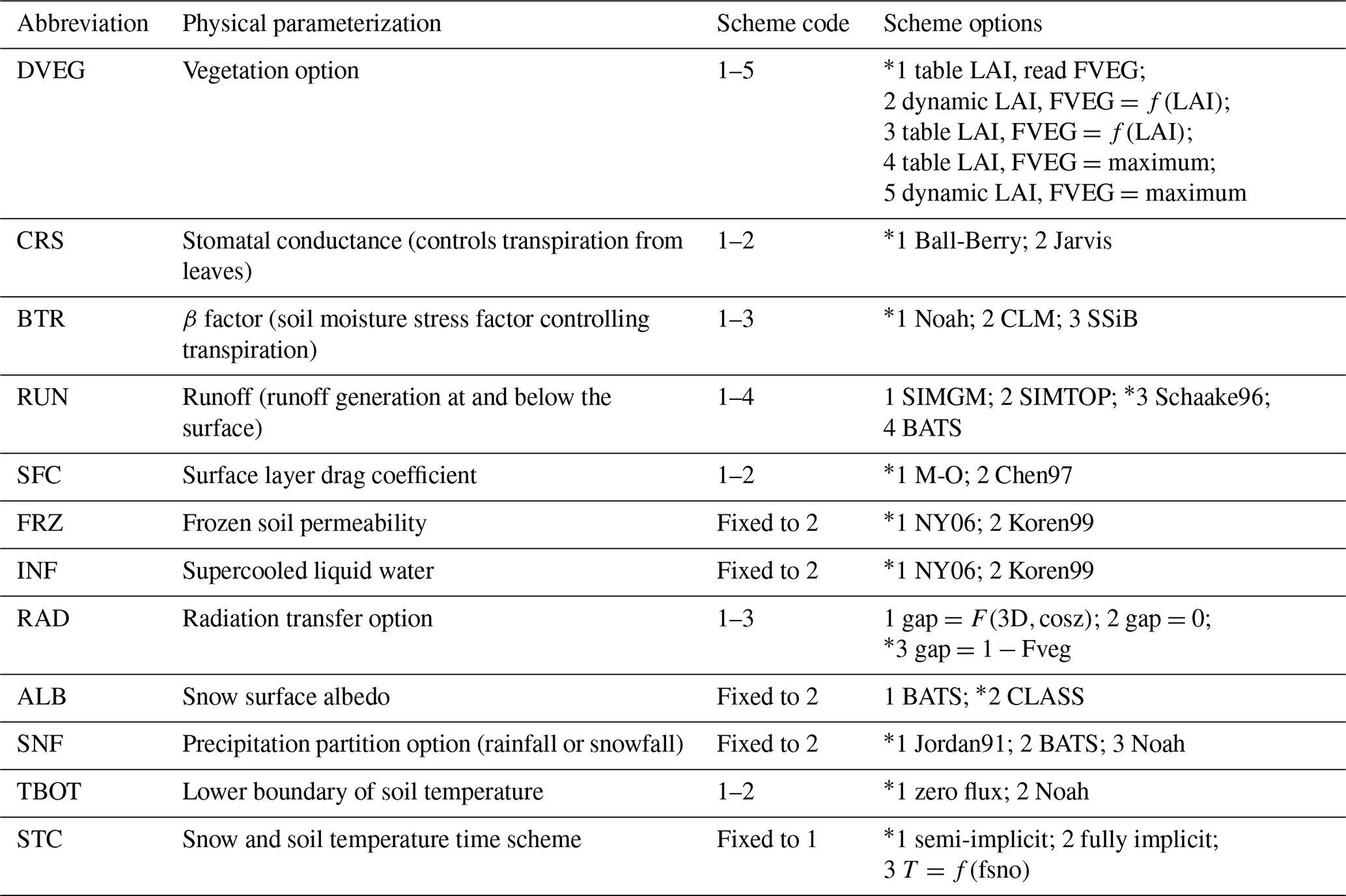
Noah-MP excels in physical representation of water and energy dynamics across various environmental layers, including a vegetation canopy layer, multiple snow and soil layers, and an optional unconfined aquifer layer for groundwater. To capture specific physical processes, Noah-MP employs multiple parameterization schemes, providing users with the flexibility to choose from a total of 12 parameterizations, as detailed in Table 1. This versatility enables tailored representation of diverse environmental conditions and processes, enhancing the model's adaptability and applicability.

Table 1 Parameterization options for Noah-MP (an asterisk (^∗) denotes the recommended default option). Certain abbreviations correspond to terms used for parameterization schemes (PSs) in Noah-MP, and their meanings can be referenced in the WRF-Hydro 3.0 user document (Gochis et al., 2015). Note that these options may not be applicable to other versions of Noah-MP, such as that used in HRLDAS. The scheme options here presented by some abbreviations such as “Noah” or “Schaake96” are those used in the “namelist” file for Noah-MP.

3 Development of NMH-CS

3.1 Translation of Noah-MP code

Our primary focus in developing NMH-CS involves translating the original Fortran code of Noah-MP into the C# language. It is essential to note that this translation is based on a relatively old version of Noah-MP utilized in WRF-Hydro 3.0, as the process was started before the release of Noah-MP 5.0 (He et al., 2023).

Converting Fortran code into C# is not straightforward due to significant syntax differences between the two languages. The reconstruction of the model in C# follows an object-oriented design. While Fortran is traditionally a function-based language, the core Noah-MP module's functions, subroutines, and state variables are encapsulated as members within a C# class named GridCell (Fig. 1a). This class represents all Noah-MP behaviors within a grid box. The variable names, function definitions, data structures, and execution logic have been kept largely consistent with the original Fortran code, ensuring user-friendliness for those familiar with Noah-MP. To handle the execution across multiple grid boxes, another C# class named Driver is employed. This class manages tasks such as initializing model variables, creating multiple grid boxes, reading and writing files, and controlling the execution of the model.

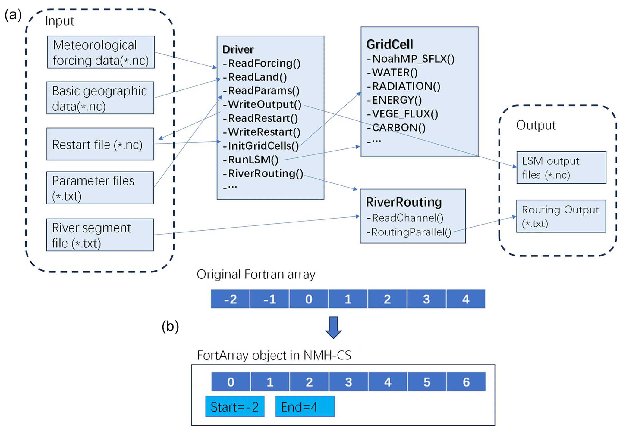
Figure 1 The architectural diagram of NMH-CS (a) and the conversion of Fortran arrays to C# arrays (b). NMH-CS is a reconstructed replica of the version of Noah-MP that is coupled in WRF-Hydro 3.0.

Throughout the translation process, a key focus was addressing operations on Fortran arrays (Fig. 1b), crucial for representing the state of soil and snow layers in Noah-MP. Unlike C#, Fortran allows arrays to have user-specified index ranges (e.g., index values from −3 to 4). However, in C#, the first index of all arrays invariably starts from 0. To streamline the translation, we designed a wrapping class of C# arrays, named FortArray, to mimic Fortran arrays. The wrapped inner-array data in FortArray adhere to standard C# conventions, accepting 0 as the inner index of the first element. Yet, externally, the class allows access to the array values through extra indices by providing methods for index translation from outer indices (Fortran style) to inner indices (C# style):

$$\begin{array}{}\text{(1)}& I_{\text{in}}=I_{\text{ex}}-I_{\text{start}},\end{array}$$

where I_in, I_ex, and I_start represent the inner index, the outer index, and the first outer index, respectively. The inner index corresponds to the standard C# arrays, while the outer index corresponds to the Fortran arrays. For instance, if a Fortran array of eight elements has an index range from −3 to 4, it will be translated into a FortArray that has a standard inner array of eight elements, accompanied by two arguments representing the starting Fortran index (−3) and the ending Fortran index (4), but the range of its inner indices remains 0–7. This array translation technique ensures that all the original execution logic in Noah-MP is seamlessly preserved in NMH-CS.

The model also supports parallel execution, implemented through the native parallel functionality of the C# language. The technique can efficiently allocate computational tasks over the grid boxes to different threads which can be executed by separate CPU cores. For instance, if a grid domain requires the execution of over 2400 grid boxes and the tasks are assigned to eight threads, each thread is responsible for the calculations applied to approximately 300 grid boxes. It is crucial to note that if the number of specified threads exceeds the number of CPU cores, several threads should be executed by the same CPU core. Therefore, specifying more threads than the available CPU cores does not contribute to an overall improvement.

3.2 Coupling with a parallel river routing module

The Noah-MP land surface model can produce column outputs of runoff but cannot simulate the horizontal movement of water. In order to simulate the surface movement of runoff in the river channels, we integrated a parallel river routing module, which is based on the Muskingum method for vectorized channel networks. The module has been described in a previous study (Liu et al., 2023). This module is not the previous RAPID model that was coupled in WRF-Hydro (Lin et al., 2018). This parallel river routing module, implemented using C#, incorporates our unique techniques.

The first technique is an array-based sequential processing method for Muskingum routing. Muskingum–Cunge equation (Cunge, 1969) with lateral inflow considered is

$$\begin{array}{}\text{(2)}& \begin{array}{rl}{Q}_{\mathrm{e},t+\mathrm{1}}=& C_{\mathrm{0}}\times Q_{\mathrm{s},t}+C_{\mathrm{1}}\times Q_{\mathrm{s},t+\mathrm{1}}\\ & +C_{\mathrm{2}}\times Q_{\mathrm{e},t}+C_{\mathrm{3}}\times Q_{\text{lat},t+\mathrm{1}},\end{array}\end{array}$$

where

$$\begin{array}{rl}& C_{\mathrm{0}}={\displaystyle \frac{kx+\mathrm{0.5}\mathrm{\Delta }t}{k(\mathrm{1}-x)+\mathrm{0.5}\mathrm{\Delta }t}},C_{\mathrm{1}}={\displaystyle \frac{-kx+\mathrm{0.5}\mathrm{\Delta }t}{k(\mathrm{1}-x)+\mathrm{0.5}\mathrm{\Delta }t}},\\ & C_{\mathrm{2}}=\mathrm{1}-C_{\mathrm{0}}-C_{\mathrm{1}},\text{and}{C}_{\mathrm{3}}={\displaystyle \frac{\mathrm{\Delta }t}{k(\mathrm{1}-x)+\mathrm{0.5}\mathrm{\Delta }t}}.\end{array}$$

Here, Q represents the channel streamflow (m³ s⁻¹), which can be considered a function of time and position; “s” is the start point of a channel segment/node and “e” denotes the end point of the channel segment, both of which are used as subscripts for different spatial positions; and t denotes the start of the period or inflow and t+1 denotes the end of the period or outflow, both of which are used as subscripts for position. The subscript “lat” represents the lateral streamflow (runoff) from the current river catchment.

Two parameters of the Muskingum–Cunge method are k and x. k is the travel time of a flow wave with celerity c_k through a channel segment of length L; thus $k=L/c_k$. Parameter x can be estimated by

$$\begin{array}{}\text{(3)}& x={\displaystyle \frac{\mathrm{1}}{\mathrm{2}}}\left(\mathrm{1}-{\displaystyle \frac{q}{S_o{c}_{k}L}}\right),\end{array}$$

where q represents unit width streamflow and S_o is the channel bed slope.

The lateral inflow of each river segment is the runoff simulated by the Noah-MP column LSM in NMH-CS, which is expressed as

$$\begin{array}{}\text{(4)}& Q_{\text{lat},t}=R_{c,t}{A}_{\mathrm{s}},\end{array}$$

where Q_lat,t is the lateral inflow at time t, R_c is the runoff value at the given grid box, and A_s is the local catchment area of the current channel segment.

The form of Eq. (2) implies that the river routing calculation can be completed from any upstream river segment to its downstream segment. At the time t+1, all the outflows ($Q_{\mathrm{e},t+\mathrm{1}}$) of multiple upstream segments will be summed as the inflow ($Q_{\mathrm{s},t+\mathrm{1}}$) of the current segment. Although a common river network is a tree-like structure, it can be represented as a sequential array, where any upstream river segment is stored near the array head (with a zero index), while its downstream river segment is stored near the array's tail (with a large index). Therefore, the Muskingum routing can be calculated over the river segment array in a unidirectional processing way (please see Fig. 1 in Liu et al., 2023).

The second technique is the straightforward equally sized domain decomposition method to conduct parallel calculation: just allocating the river segments into equally sized blocks. Within each block, the Muskingum routing can be executed separately by a single CPU core. This treatment is based on the assumption that in any block, most segments have upstream segments within the same block and only a small fraction of the segments have upstream segments in other blocks. Therefore, all river segments that receive inflows from other blocks (referred to as “cross-block segments”) need to be identified. These cross-block segments should be executed by the primary core, after the multi-domain parallel execution is completed.

The third technique is a specific sorting approach for river segments used in domain decomposition. It has been proven that a depth-first traverse of the river segments is more suitable, compared to a width-first traverse, for the parallel execution of the Muskingum method due to fewer cross-block segments in the blocks.

This module requires two additional inputs files, a river segment list file named “ChannelOrder.txt” and a “namelist.txt” file. The latter file is used to set parameters and the length of time steps. Each river segment in the list file presents the following information: its own index, the index of its next downstream river segment, the row number and the column number of the grid box (in Noah-MP's running domain) providing runoff input to the current segment, the length (m) of the current river segment, the two parameter values (K and X) of the Muskingum method, and the area of the catchment of the current segment.

The river segment list can be derived from both the gridded river network and the vectorized river network. The resolution of the river routing is determined by the original river network from which river segments are derived. Therefore, the choice of using the vector river network or gridded river network and the selection of spatial resolution are completely determined by the users. The length of the temporal step of the river routing is required to be multiple times shorter than the time step for running the Noah-MP and can also be designated by the users. For example, the time step of routing is set to 600 s, while the time step for the Noah-MP LSM is usually set to 3 h.

This approach's primary advantage lies in its ability to simply decompose any river network into multiple domains with an equal number of river segments. Achieved by evenly dividing the river segment list into any number of blocks, this innovation capitalizes on the inherent tree-like structure present in most river networks. Importantly, it does not necessitate consideration of the topological conditions specific to a given network, as required in studies such as those of Mizukami et al. (2021) or David et al. (2015). This design allows the parallel execution of river routing on modern personal computers equipped with multi-CPU cores.

The integration of the river routing module with the Noah-MP LSM involves assigning lateral inflows from the LSM-simulated total runoff to the river routing model. In the present NMH-CS configuration, we utilize a catchment centroid-based coupling interface (David et al., 2015). This method designates the LSM grid cell containing the catchment centroid (referred to as the “centroid cell”) as the location for a river reach to receive lateral inflows. At a specific temporal step, the computed contributing runoff discharge Q_lat (unit: m³ s⁻¹) is determined by the following expression:

$$\begin{array}{}\text{(5)}& Q_{\text{lat}}=R(nx,ny)\times F\times \mathrm{1000},\end{array}$$

where R(nx,ny) is the runoff (mm, surface + subsurface) simulated by the LSM during the time step and F is the catchment area (km²) contributing water to the current river segment.

Alternatively, employing weighted assignments from different grid boxes, akin to the method utilized in Lin et al. (2018), is also a valid approach. However, this method requires the generation of weights from multiple grid boxes. Given the rough resolution of the meteorological datasets, each grid box can encompass the catchment areas of multiple river segments; the coupling approach using area weighting is unlikely to yield substantial improvements for most river segments.

3.3 Code debugging process

To eliminate any potential code errors resulting from incorrect translation, we conducted a thorough check of the code by performing model execution benchmark tests on single columns running on specific grid boxes. Here, In the large domain (the same domain described in Sect. 4.1), the grid box for single-column execution is arbitrarily selected each time. Such debugging tests were carried out in two approaches. The first approach was to carry out meticulous step-by-step debugging by examining the printed values of many variables (including many local variables in the code) in WRF-Hydro 3.0. This process was also repeated by switching each option of multiple physical parameterization schemes. The grid box for the single-column debugging was also switched several times. Such debugging has been conducted numerous times and has effectively eliminated any code errors arising from inaccurate translation. Although meteorological driving data for the debugging simulation are prepared for the period between 2000 and 2016, such debugging tests are only feasible for a limited number of temporal steps for a grid-box execution. It is also impossible to conduct debugging on the entire domain.

The second approach is an artificial code-checking process. Considering that the stepwise debugging through years-long simulations is impractical, we checked the NMH-CS's code by comparing it with the original Fortran code many times. Through this checking, many code inconsistencies were identified and corrected.

4 Testing of NMH-CS

4.1 Application area and data

4.1.1 Application area

The Yellow River basin in northern China is used as a test area of NMH-CS. The gridded domain, as illustrated in Fig. 2a, encompasses the entirety of the Yellow River basin (YRB) and most of northern China, comprising 350 columns and 170 rows, with a 6 km resolution in Lambert conformal conic projection coordinates. Geophysical data essential for the domain, including digital elevation, land use and land cover, and the green vegetation fraction, were extracted from the WRF/WPS 3.5 input database.

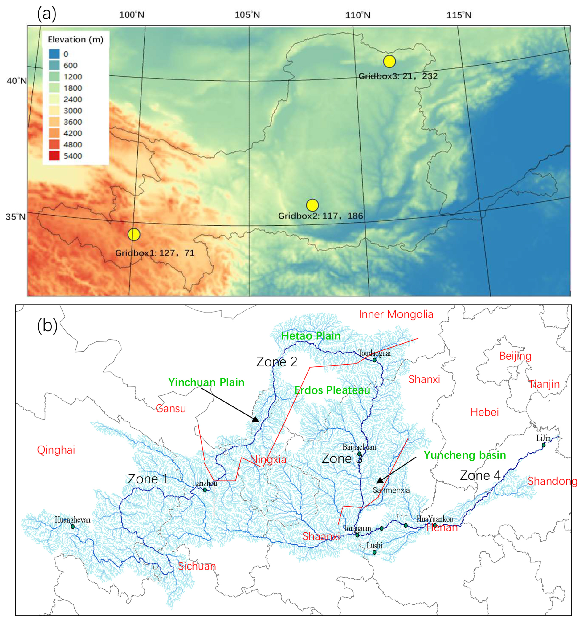
Figure 2 The terrain map of the simulation domain (a) and the vector river network utilized for river routing modeling (b). The three grid boxes used for extracting state variables for comparison are represented by yellow dots on the terrain map (a) and are labeled with the grid-box code, row numbers, and column numbers. The grid domain covers the Yellow River basin and the northern China area. The vector river network utilized for river routing modeling was extracted from the HydroSHEDS dataset. The delineation of the boundaries between different zones controlled by four gauging stations (Lanzhou, Toudaoguai, Sanmenxia, Lijin) is indicated by red lines.

For the river routing simulation, the digital river network of the Yellow River was obtained from the HydroSHEDS dataset (version 1) (http://hydrosheds.cr.usgs.gov/, last access: 1 September 2016). HydroSHEDS was derived from gridded digital elevation data with a resolution of 15 arcsec. Given substantial human intervention in the area and the intricate nature of reproducing observed daily or hourly water discharge, uniform values were assigned to all river segments for the river routing parameters (specifically, the wave celerity (c_k) and another parameter (x) describing the river channel condition, as detailed in David et al., 2013). No precise calibration is required here, as monthly or annual river discharge remains unaffected by changes in routing parameters.

The Yellow River basin experiences significant human impacts, including irrigation, industrial water usage, and groundwater extraction. Major artificial reservoirs and numerous smaller reservoirs regulate the river's discharge, serving as the primary water resource during the dry season. However, such extensive human interference presents substantial challenges in accurately modeling river discharge. Comparatively, the river discharge upstream of the Lanzhou hydrological station (in Zone 1 as shown Fig. 2b) contributes over half of the entire YRB's total discharge and is less impacted by dams, enabling us to test the model's performance.

4.1.2 Meteorological dataset and river discharge data

To drive the two models (NMH-CS and WRF-Hydro), the same 3-hourly and 6 km gridded meteorological forcing dataset comprised of the shortwave and longwave downward radiation, wind velocity, air temperature, relative humidity, air pressure at the surface, and precipitation rate was acquired. The benchmark dataset was clipped and regridded (bilinear interpolation) from the 1.0°×1.0° GLDAS-1 land surface product (Gan et al., 2019; Rodell et al., 2004) for the period 2000–2016. Given the limited availability of observational river discharge data between 2001 and 2016, the extracted data pertain to this period, and additional data between 1996 and 2000 were also extracted for the model's spin-up.

In previous research, the spin-up of Noah-MP has required 50 years (Wu et al., 2021) or more than 100 years (Zheng et al., 2019) to achieve an equilibrium state. However, in this study, the spin-up process was conducted in two steps. In the first step, the period from 1996 to 2016 was run three times to generate a “restart file” for a 63-year spin-up, utilizing the initial PS combination. In the second step, starting from this initial combination, new schemes were adopted, and the restart file obtained from the initial scheme combination was used to initiate the formal experiments covering the period from 1996 to 2016.

The dataset of Natural River Discharge (RND) reconstructed by the Yellow River Conservancy Commission of the Ministry of Water Resources was used to assess the model output. Annual natural discharges from the monitoring station of Lanzhou were collected for the period from 2001 to 2016.

4.2 Running speed

Compared to other differences between the two models, running speed is the least important factor to consider. Considering that NMH-CS and WRF-Hydro run on different platforms (Windows or Linux) and machines, it is also difficult to achieve a comparative evaluation of running speed. Actually, the comparison of running speed depends on the programming language used. In theory, Fortran and C programs can run faster than C# programs because Fortran and C are relatively low-level languages compared to any modern object-oriented language. However, as a language that can run in native machine code, C# is not slow. This means that there will not be a large difference in running speed between C# and Fortran. There are few authoritative publications on the running speed of these two languages, but there are many documents on benchmark testing on the internet. When considering parallel execution, comparing the running speed of the two models also becomes less necessary. NMH-CS can run in parallel mode on personal computers, while WRF-Hydro does not have this functionality. On the other hand, WRF-Hydro can run in parallel mode in the Message Passing Interface (MPI) environment of high-performance computers, while NMH-CS does not support MPI.

We tested the execution time of NMH-CS by setting different numbers of C# parallel threads. The computer used for the testing is a common laptop with six CPU cores. The results indicate that for the execution of the entire domain, as the number of threads increases from 1 to 6, the average time consumed per time step is 1576, 977, 801, 711, 679, and 672 ms, respectively. When the number of threads is set to 1, the time spent is slightly greater than the execution time in the non-parallel mode (1461 ms). It is worth noting that the time spent is not linearly related to the number of parallel threads, which can be explained by various reasons. One is that some tasks are not actually executed in parallel mode, such as reading meteorological input files. Another reason is that not all threads in NMH-CS are fully processed by the CPU cores, as there are many other tasks in the entire Windows environment that have to be processed simultaneously by the CPU cores.

4.3 Comparing the outputs of NMH-CS and WRF-Hydro

It is noteworthy that there are numerous parameterization scheme combinations for Noah-MP, which makes it unfeasible to compare the results generated under all scheme combinations. Therefore, the output of NMH-CS and WRF-Hydro was compared only with the default parameterization scheme combination, based on the exact same meteorological dataset. The comparison was conducted in two ways. The first comparison is that of the spatial maps of multiple variables (Table 2) for a specific year or day. For each state variable, such as SFCRNOFF, the maps of state variables simulated by NMH-CS and WRF-Hydro are presented. The difference (Δ) between the values of the same variables simulated by the two “Noah-MP models” is calculated as

$$\begin{array}{}\text{(6)}& \mathrm{\Delta }=V_{\text{NMH-CS}}-V_{\text{WRF-Hydro}},\end{array}$$

where V_NMH-CS and V_WRF-Hydro are the state variable simulated by the two Noah-MP models, respectively.

For certain variables, such as SFCRNOFF, UGDRNOFF, ECAN, and ETRAN, the percent relative differences were also calculated as follows:

$$\begin{array}{}\text{(7)}& \mathit{\delta }=\mathrm{100}\times \mathrm{\Delta }/V_{\text{WRF-Hydro}}.\end{array}$$

The second method is to compare the temporal variations in state variables for specific grid boxes. In this case, only three grid boxes (Fig. 2) were selected to extract the state variable time series. The selection of these grid points is an arbitrary decision made by roughly considering different climate zones without other strict considerations. Gridbox1 is selected from the Qinghai–Tibet Plateau region, corresponding to the source region of the Yellow River. Gridbox2 corresponds to a location of Inner Mongolia and the north of the Loess Plateau. Gridbox3 is in a hilly area of the Wei River basin (a major part of the Yellow River basin). In fact, during this study, other grid points were also casually tested, but the results for these were mostly similar to the three above-mentioned grid boxes and will not be presented in the paper.

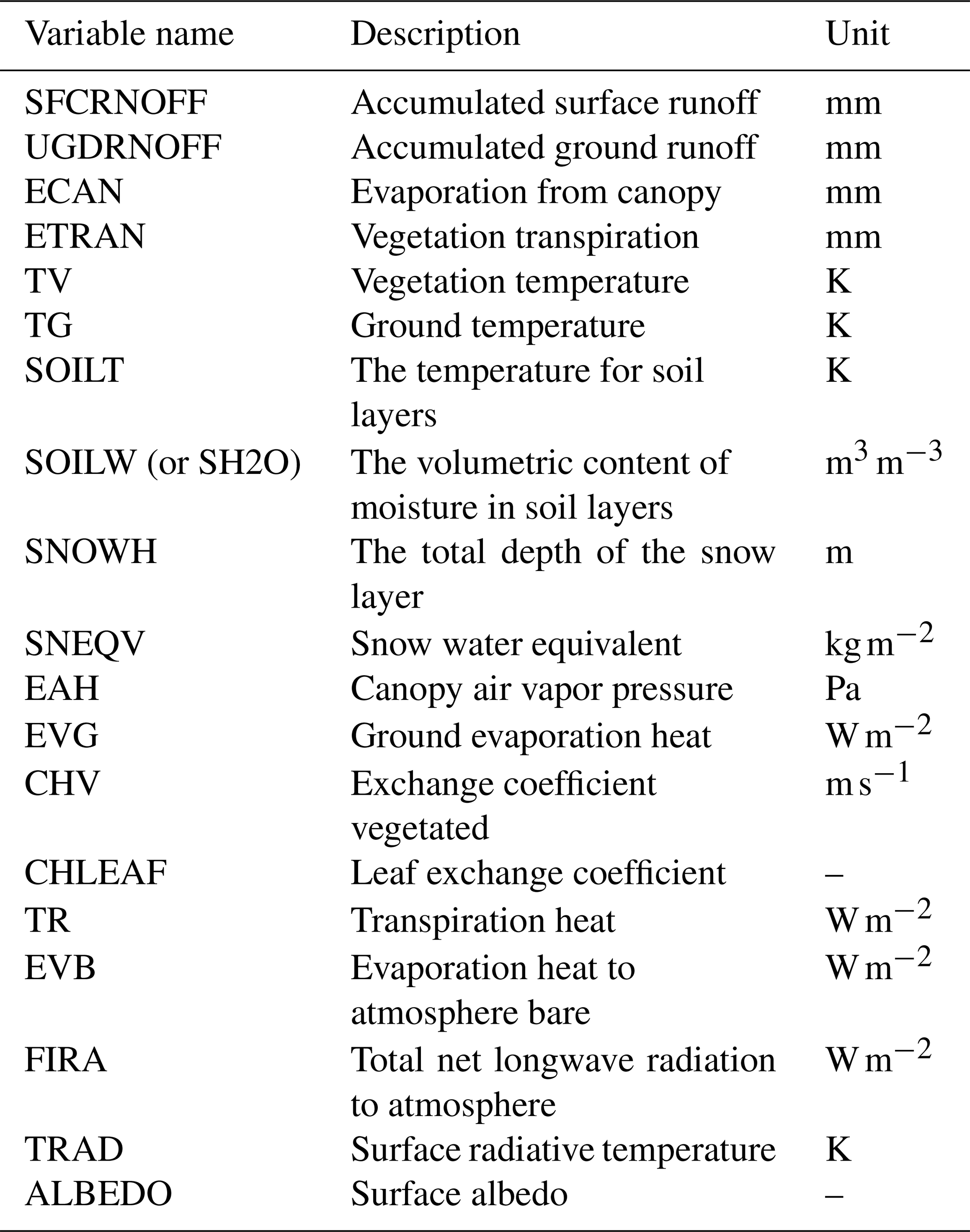
Table 2 The state variables simulated by NMH-CS and WRF-Hydro, which are verified by generating maps.

4.3.1 Maps of state variables

To test whether NMH-CS can produce the corresponding outputs of the original WRF-Hydro (Noah-MP Fortran version), many state variables (Table 2) from multiple time slices have been checked by drawing maps. Only four slices (10 June 2000, 10 June 2001, 10 June 2004, and 10 June 2008) were arbitrarily selected here without special consideration. Only some maps of these state variables at certain time slices are presented in both the paper and the Supplement. The maps for all the state variables in Table 2 reflect high consistency between NMH-CS and WRF-Hydro, with only the maps for four representative variables (SFCRNOFF, UGDRNOFF, TV, and TG) shown in Figs. 3 and 4.

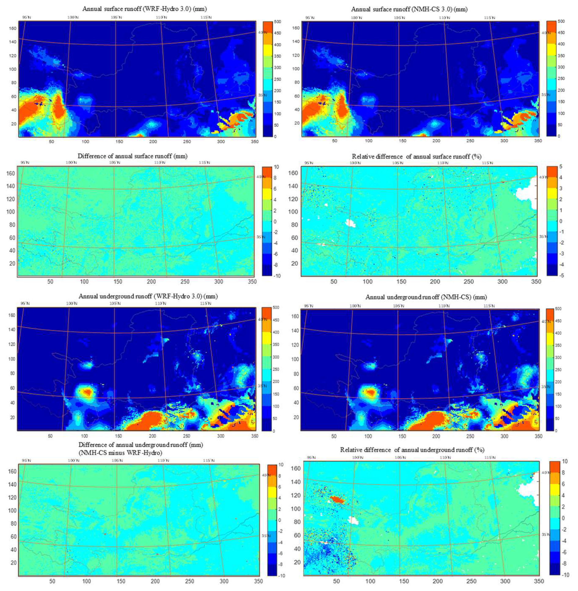
Figure 3 Maps of annual total values of, differences in, and relative differences in SFCRNOFF (surface runoff, mm) and UGDRNOFF (underground runoff, mm) simulated by WRF-Hydro3.0 and NMH-CS 3.0 for the year 2005. The labels for the horizontal axes and vertical axes are row numbers and column numbers of the grid domain, respectively.

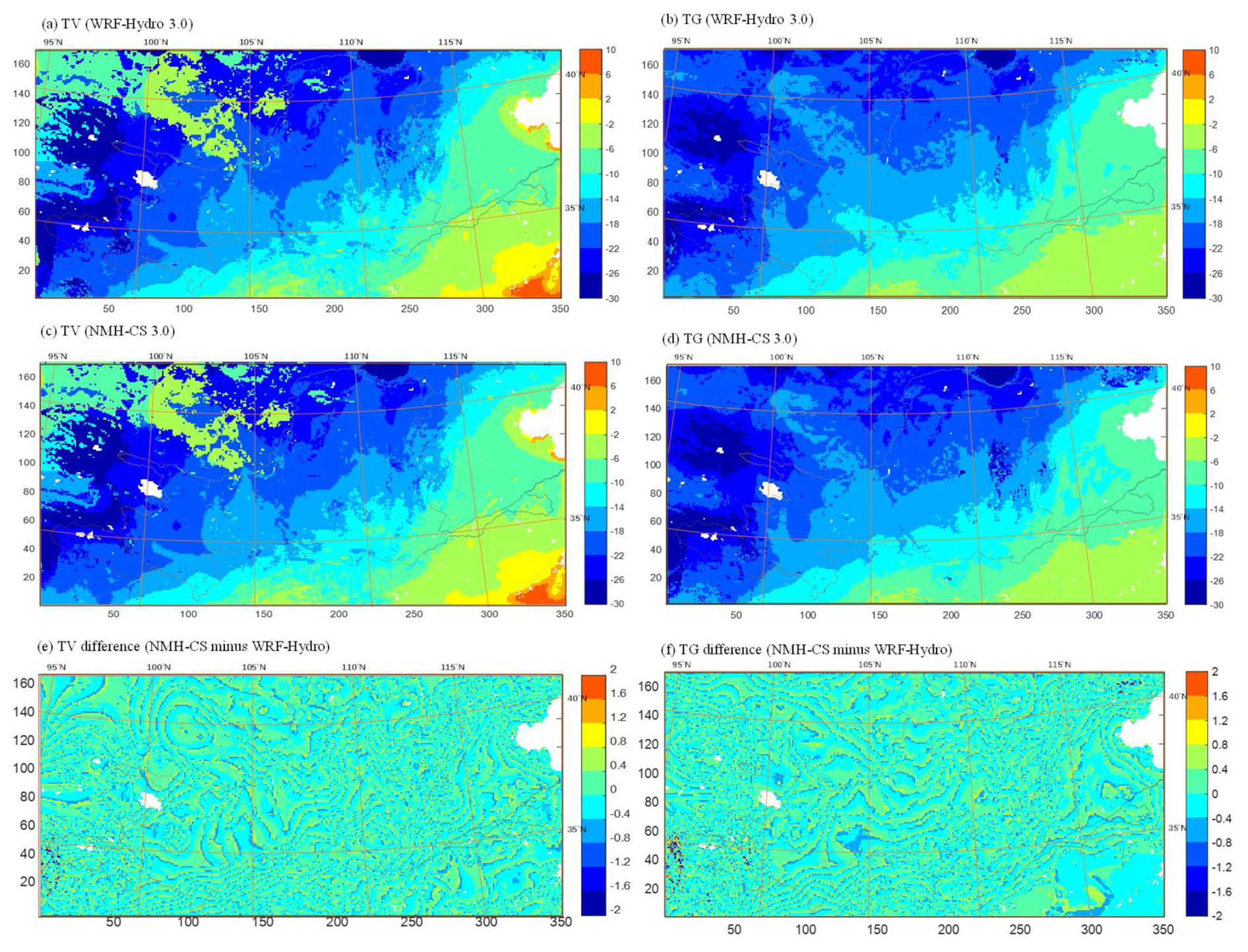
Figure 4 Similar to Fig. 3 but showing the maps for TV (vegetation temperature, °C) and TG (ground temperature, °C) for 1 January 2008.

As can be seen, there is visually little difference in the spatial patterns of the results. Similarly, no discernable visual difference is apparent for the maps of other variables. However, the relative difference in annual surface runoff and annual underground runoff is significantly large in some areas (generally in high-elevation regions), where NMH-CS underestimated/overestimated those values above 10 % (Fig. 3). These regions with large relative differences in underground runoff actually have small absolute differences, primarily because the annual total groundwater runoff in these areas is inherently low (<50 mm). This discrepancy is likely attributable to floating-point arithmetic errors, but the possibility of other contributing factors cannot be ruled out.

For most of the domain, the difference in TV is smaller than 0.2 °C, but in some sporadically distributed locations, the TV's difference can be larger than 2 °C (Fig. 4). The comparison of TG shows similar effects, but the difference is more significant than that of TV. Similar high-consistency effects are also reflected by other state variables, including soil temperature, soil water content, and snow water equivalent (Figs. S2–S4 in the Supplement). The differences in these state variables between the two models are generally small, except some large ones are sporadically distributed in the high-latitude areas.

4.3.2 Temporal variations in state variables

The outputs at the three representative grid boxes (as shown in Fig. 2) indicate that the two models produced consistent temporal changes (Figs. 5 and S5 and S6 in the Supplement). For certain variables, for example, SFCRNOFF, TV, and TG (other variables as well), occasionally, some significant differences were found in certain months for Gridbox2. It must be such occasional differences that caused the spatial disparity shown in Figs. 3 and 4. We checked the disparity for certain grid boxes and the 3-hourly values and found that the differences also happen sporadically (Fig. 6). Almost all the disparities occur during the cold months (November, December, January, and February). However, it is worth noting that the simulated state variables in these months mostly show no difference. Considering such a mismatch usually happens in cold months and high-elevation regions, it may be caused by the different calculation accuracy for the processes of snow or frozen soil. For the three representative grid boxes, no significant differences were identified for certain variables, including many variables like TR, EAH, TV, ETRAN, and UGDRNOFF (no plots for these variables will be presented in the paper).

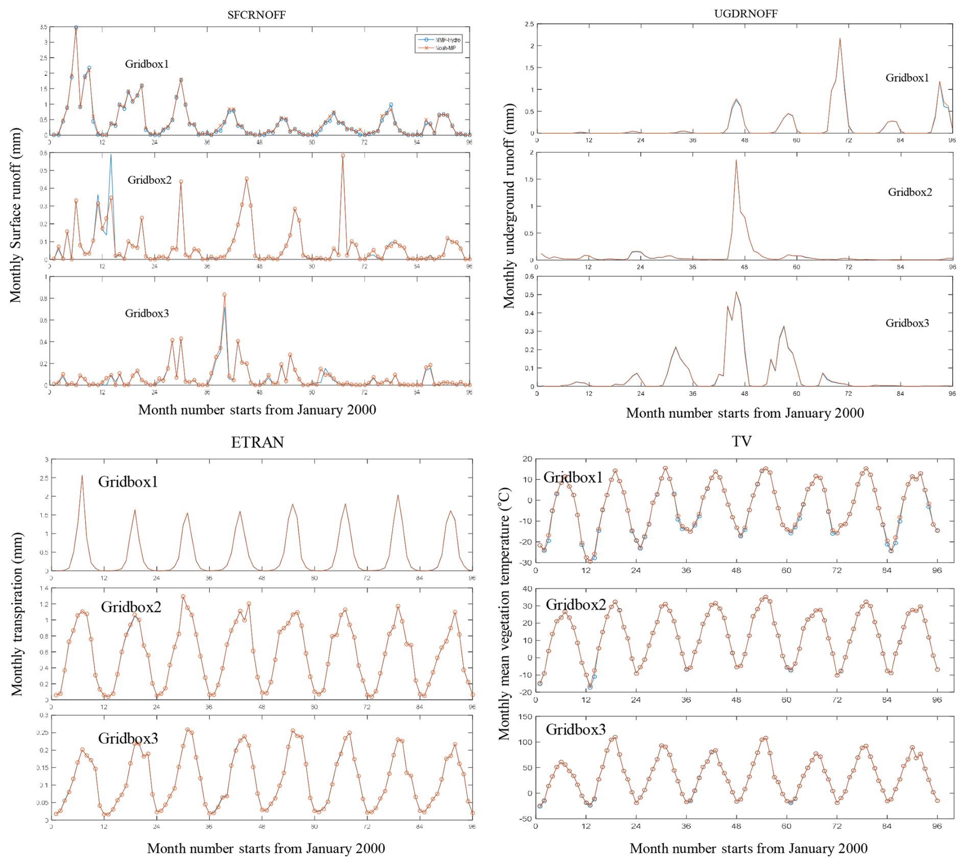
Figure 5 Monthly surface runoff (SFCRNOFF in mm), underground runoff (UGDRNOFF in mm), transpiration (ETRAN in mm), and vegetation temperature (TV in °C) simulated by WRF-Hydro3.0 (blue) and NMH-CS (red) for the three grid boxes, 2000–2007.

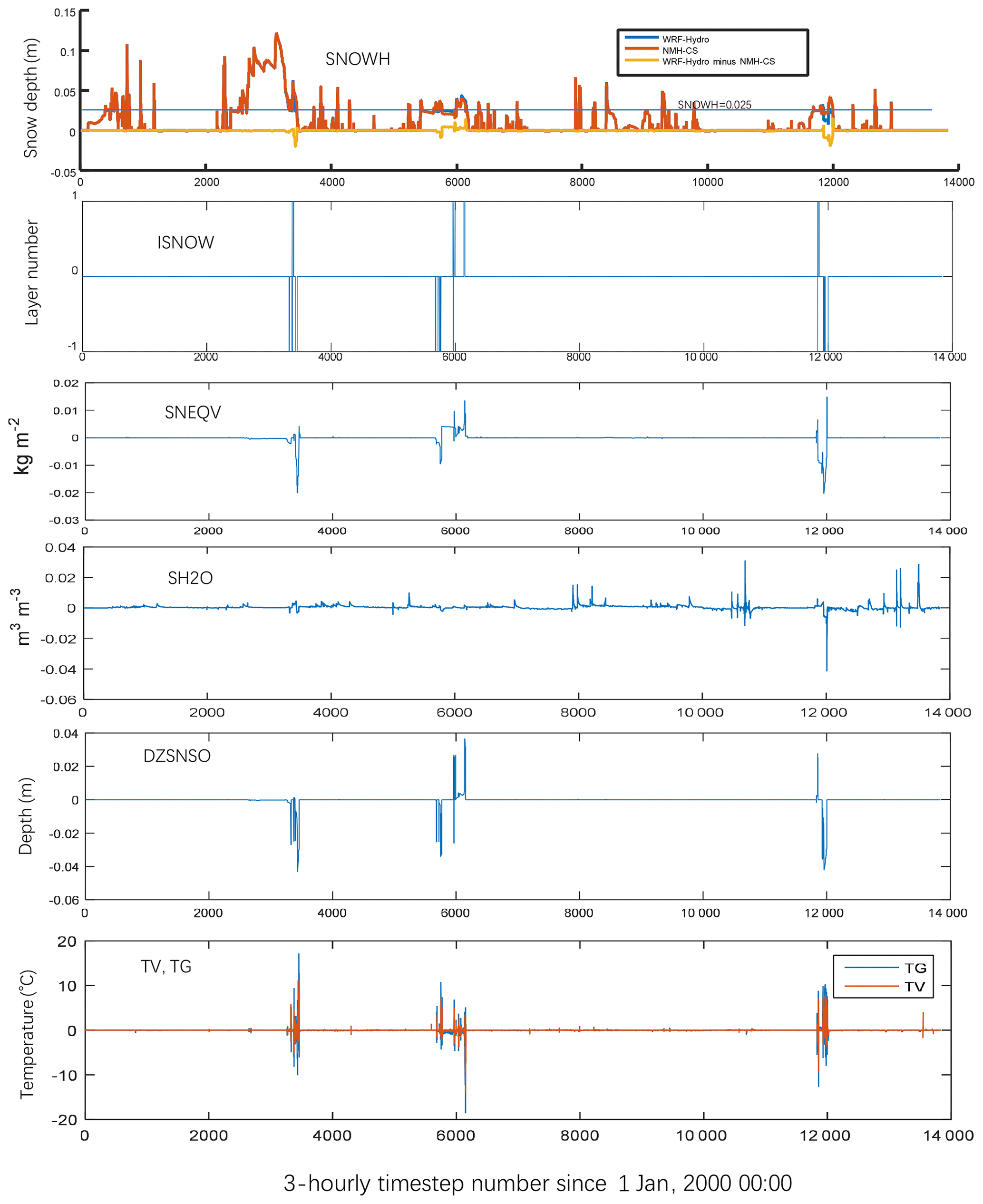
Figure 6 The differences (NMH-CS minus WRF-Hydro) between the 3-hourly variables simulated by NMH-CS and those simulated by WRF-Hydro. SNOWH: snow depth (m); ISNOW: number of snow layers, count; SNEQV: snow water equivalent (kg m⁻²); SH2O: soil liquid water content (m³ m⁻³), equivalent to SOILW; DZSNSO: snow and soil layer depth (m). These variable names are those used in the programming code. The occurrence of the three inconsistencies corresponds to the short periods: 4 March 2001, 15 January 2002–8 February 2002, and 22 January 2004–9 February 2004.

By comparing and analyzing the printed state variables (in 3-hourly time steps) in WRF-Hydro and the NMH-CS, we found that the major inconsistencies occur in the module of snow water (named “SNOWWATER” in the code). From Fig. 6, it can be seen that three major inconsistencies simulated between the two models occur usually simultaneously in the multiple state variables. These three cases demonstrate that almost all the major inconsistencies in multiple variables are caused by the minor inconsistencies in SNOWH (the state variable to indicate the depth of snow). The logic of the snow process in Noah-MP is coded as when SNOWH is below 0.025 m, ISNOW (a state variable to indicate whether a snow layer exists) is set to zero (no snow layer), and otherwise, it is set to 1 (having a snow layer). Therefore, if SNOWH simulated by NMH-CS is close to 0.025, a small floating-point error may trigger a division between having a snow layer and no snow. Due to the different physical effects of the radiation balance between snow layers and the ground, the distinction between having a snow layer and no snow layer will further lead to significant inconsistencies in snow depth (SNOWH), snow water equivalent (SNEQV), soil water (SOILW), vegetation temperature (TV), and ground temperature (TG). Once an inconsistency occurs, it will persist for a period of time. It is highly probable that the minor differences in SNOWH are caused by accumulation of floating-point error because, most of the time, the differences are very small except those during the inconsistent periods. This explanation may account for the inconsistencies observed in the time series in Fig. 6 and the sporadically distributed discrepancies in high-latitude regions depicted in Fig. 4.

The daily time series from multiple grid boxes (including the three marked in Fig. 2) were extracted and compared between NMH-CS and WRF-Hydro. Similar effects were obtained for the grid boxes, but only the results for Gridbox3 are presented as representative in Fig. 7. It is evident that the rate of direct evaporation from soil (EDIR), SFCRNOFF, soil water content (SOILW), and TV exhibit small discrepancies, whereas TG demonstrates large disparities. The daily samples for soil temperature, soil water content, snow depth, and snow water equivalent are presented in Figs. S1, S5, and S6 in the Supplement. The comparisons of soil layers reflect the fact that the soil temperature has relatively large inconsistencies, which should also be explained by the different division of snow layers that is caused by error when SNOWH approaches 0.025 m.

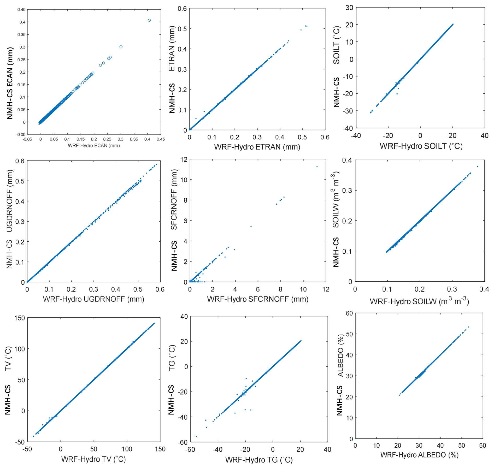
Figure 7 Daily state variables simulated by NMH-CS versus by WRF-Hydro at Gridbox3. Due to the high consistency for most of the values, statistical evaluation metrics such as correlation coefficients or relative biases will not be presented in the paper.

4.4 Streamflow discharges for the Yellow River by NMH-CS

4.4.1 Experimental design of the Noah-MP simulation

Here, we present the numerical outputs of NMH-CS applied to the streamflow discharges over the Yellow River, with various parameterization schemes used. To verify whether the various parameterization schemes (PSs) of NMH-CS can produce reasonable discharge values for the Yellow River catchment area, this study conducted 17 Noah-MP simulations using different PS combinations. Given the challenge of determining the relative importance of each parameterization and the impracticality of including all possible combinations, we adopted a strategic approach. A fixed PS combination was established as a foundation, and alterations were made to one parameterization's scheme at a time (refer to Table 3).

Table 3 Experiments conducted in this study.

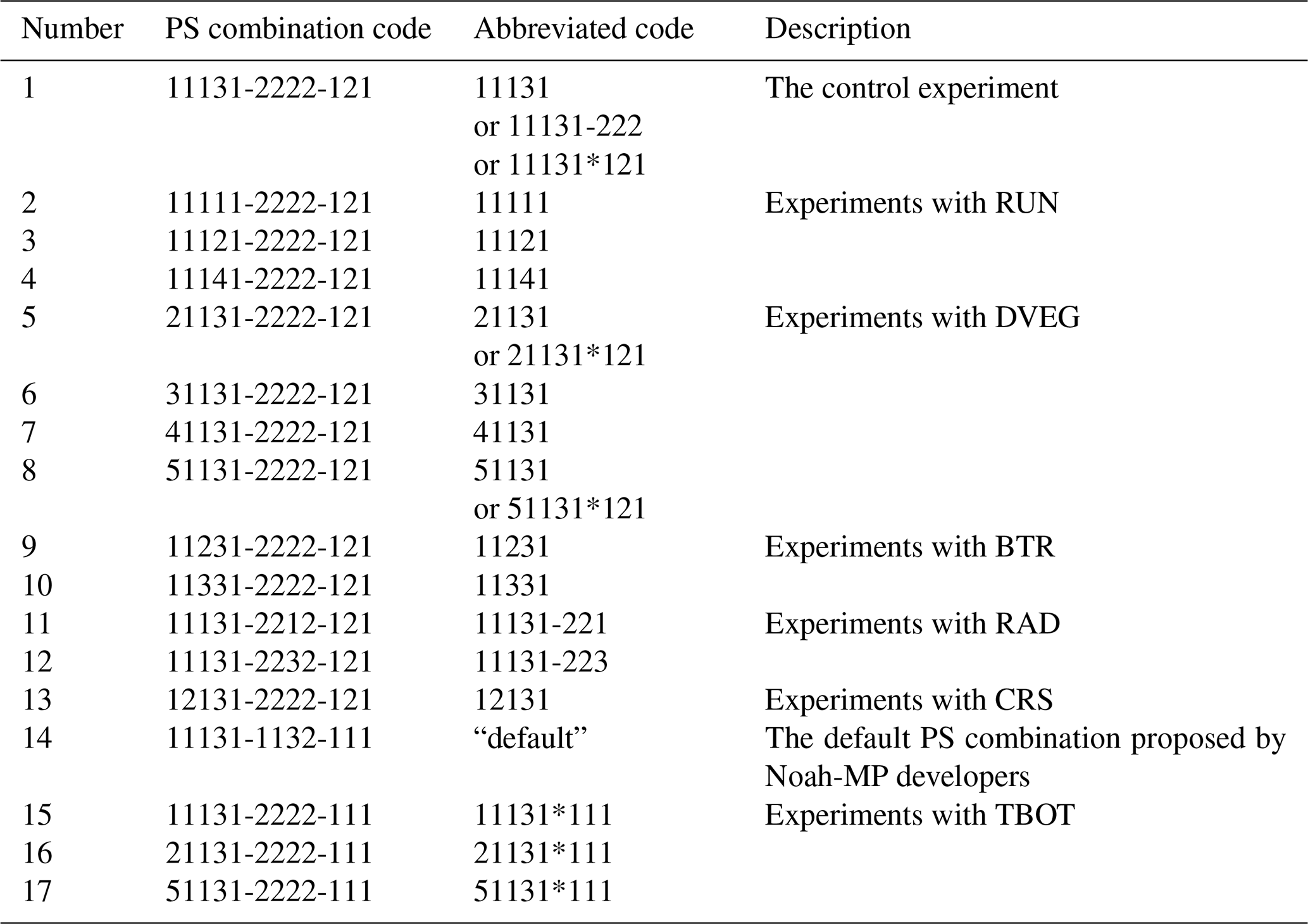
In addition to our selected parameterizations, we considered commonly used PS combinations, including the “default” combination proposed by Noah-MP developers. Sensitivity analysis was conducted by analyzing the differences or variations among these incomplete PS combinations. It is important to note that the chosen PS combinations represent only a subset of all possible combinations, and the assumed sensitivities based on this subset are considered indicative of overall sensitivities based on the complete set of combinations.

The PS combinations are represented by codes consisting of sequential digital numbers. For instance, the default combination is denoted “11131-1132-111”, where each number signifies a scheme option. The initial experiment, arbitrarily set as the PS combination of “11131-2222-121”, served as the foundation for subsequent experiments. A total of 16 experiments (refer to Table 3) were then conducted by modifying one option at a time compared to the initial experiment.

These experiments are categorized into multiple groups, with the initial experiment “11131-2222-121” being employed in several of these groups:

• runoff scheme group (four experiments, switching between 1 SIMGM, 2 SIMTOP, 3 Schaake96, and 4 BATS),

• vegetation scheme group (five experiments, switching between the first option and the fifth option; see Table 1),

• β-factor option group (three experiments, switching between Noah, CLM, and SSiB),

• radiation transfer option group (three experiments, switching between three options),

• group for the scheme of the lower boundary of soil temperature (six experiments),

• group for the stomatal conductance scheme (two experiments, switching between two options).

4.4.2 Simulated streamflow under various parameterization schemes

The Taylor diagrams (Taylor, 2001) are used to evaluate the different PSs applied to the river discharge at the Lanzhou station. A Taylor diagram provides a graphical representation of a model's simulation performance, encompassing three key indices: the correlation coefficient (R), root-mean-square error (RMSE), and standard deviation (SD).

The streamflow discharges were produced by coupling the NMH-CS with the parallel river routing model. A preliminary comparison of the various scheme combinations is presented in Table 4. The monthly performance is summarized in Table 4 based on the comparison of the different PSs, as shown in Fig. 8a. It can be observed that for the majority of parameterizations, the discharges in winter are not sensitive to the schemes; this is to be expected, given the minimal runoff during this season. The simulated summer discharges exhibit a notable degree of sensitivity with regard to the various parameterization schemes. In relation to the runoff parameterization, the results obtained through the utilization of the SIGGM scheme led to overestimation during the winter season and underestimation during summer, signifying that considering groundwater could enhance the simulation accuracy of the catchment modulation when using this scheme as opposed to other schemes.

Table 4 Performance of various parameterization schemes applied to monthly discharge for the Lanzhou station.

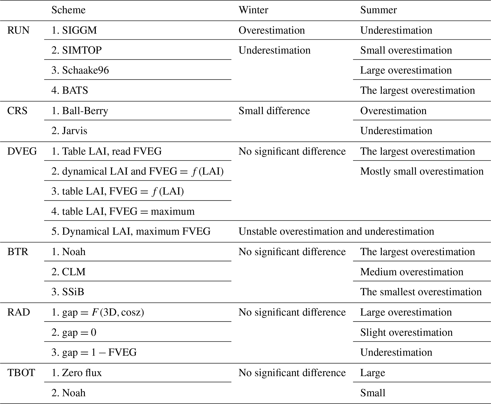
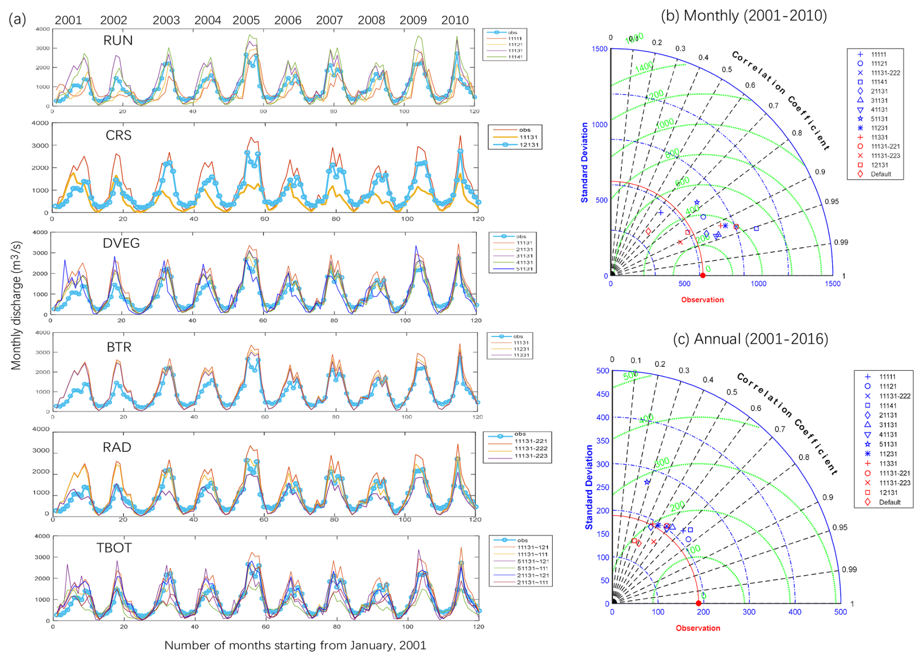
Figure 8 Monthly river discharge (m³ s⁻¹) (a) and Taylor diagrams for monthly (b) and annual (c) mean river discharges (m³ s⁻¹) for the Lanzhou monitoring station, simulated by NMH-CS. The first panel in (a) displays the results simulated with varying RUN schemes, and the other subplots follow a similar pattern. Reconstructed natural discharge is denoted “obs”.

For the Lanzhou station, over 50 % of experiments produced discharges with correlations larger than 0.9 (Fig. 8b and c). The PS combination 11141-2222-121 yielded the highest correlation, and 11131-2222-111 showed the highest performance according to Taylor's score.

5 Discussions

5.1 Major advantages of NMH-CS

The original intention of developing a Noah-MP model with the C# programming language was to analyze and edit Noah-MP code in a more efficient way, as there are many modern and efficient tools available for analyzing code written in C#, such as Microsoft Visual Studio or SharpDevelop (https://github.com/icsharpcode/SharpDevelop, last access: 20 October 2024). There are almost no comparable powerful tools for analyzing Fortran code. This advantage of C# is significant from the developers' perspective.

From the user's perspective, NMH-CS runs on Windows (although it should also run on other UNIX-like platforms after some specific configuration in the future), which is more favorable for many Windows users around the world. In the Windows system, in most cases, the NMH-CS software can be distributed across multiple computers by simply copying it; this is unlike UNIX-like systems, where compiling of the code is usually required.

5.2 Inconsistencies between the two models

As indicated by the previous analysis, the main inconsistency between the outputs of the two models (WRF-Hydro and NMH-CS) was found to be related to the transition between the presence or absence of snow layers. In Noah-MP, the existence of snow layers is determined by the depth of the snow (represented by the variable SNOWH in the code). When the SNOWH value approaches the threshold (0.025 m), a small error will result in a division on the judgment of whether a snow layer exists. This inconsistent division will further lead to significant differences in other state variables. Nevertheless, this difference will not last long (as shown in Fig. 3, up to 30–40 d). However, it is difficult to determine whether the errors in SNOWH are caused by the accumulation of floating-point errors or other errors.

There may be some other inconsistencies that have not been identified. Due to the complex nature of Noah-MP, it is challenging to identify all the minor differences through the process of code checking and debugging. Therefore, ensuring the results of two models are completely consistent needs a long-term process. Discrepancies can arise from multiple factors, including floating-point calculation errors, some inconsistent hardcoded parameter values (such as local variables in certain modules), or inconsistent programming code. The two former factors are reasonable and acceptable, whereas a coding mismatch can cause unexpected outputs. From a scientific perspective, these minor differences between NMH-CS and WRF-Hydro are not very critical, as the model users are always modifying the code during their research, and small changes in the code can lead to results with large differences. The existence of differences does not always mean that NMH-CS is inferior to Noah-MP in WRF-Hydro 3.0.

In most cases, identifying discrepancies is only feasible during the debugging of the first one to three time steps and not for tens to hundreds of subsequent iterations. It is not uncommon for errors to remain undetected even after the execution of numerous time steps. In this study, given that no code inconsistencies were found after multiple rounds of code checking, it is plausible that floating-point errors related to SNOWH (or other related variables) play a major role in explaining the remaining discrepancies.

Based on the debugging process, we also found that some variables such as TV and TG calculated by the two models always have slight inconsistencies, but they are almost insignificant on a daily or monthly scale. It is highly probable that such inconsistencies arise from the accumulated error caused by the recursive calculation of energy transfer for vegetated and bare land.

6 Model code and technical documentation for NMH-CS

We archive, manage, and maintain NMH-CS at https://github.com/lsucksis/NMP-Hydro (last access: 22 May 2025) for public access. A technical description is provided at the same site. The original version of the model is also provided at the website of the Science Data Bank: https://doi.org/10.57760/sciencedb.16102 (Liu, 2024b).

7 Conclusions

This study presents NMH-CS 3.0, which is a reconstructed land surface ecohydrological model based on Noah-MP. The model was developed by translating the Fortran code of Noah-MP (in WRF-Hydro 3.0) into C# and also by coupling it with a river routing model. The model has been designed for parallel execution on Windows systems, thereby capitalizing on the multi-core CPUs that are now a standard feature of personal computers. The NMH-CS code has been subjected to rigorous testing to ensure that it produces results that are as consistent as possible with those of the original WRF-Hydro. The code is based on the C# language, which facilitates greater user-friendliness and modification and expansion.

The development of this software enabled the successful execution of high-resolution 6 km simulations for a rectangular region covering the Yellow River basin and northern China. These simulations were conducted with a multitude of parameter scheme (PS) combinations within the Noah-MP framework. Maps of all the outputs (runoff, evaporation, groundwater, energy, vegetation) across the grid domain demonstrate consistent spatial patterns that are simulated by the two models. The long-term variations in multiple state variables simulated by the two models also exhibit high consistency, although some differences also exist. By enabling the coupled river routing model, the river discharge simulated by NMH-CS 3.0 based on the multiple scheme combination of parameterizations is found to be in reasonable agreement with the reconstructed natural river discharge for the Lanzhou hydrological station.

The main inconsistencies in multiple variables between NMH-CS output and WRF-Hydro output were found to be related to inconsistent judgments on the presence of snow layers, which are caused by minor cumulative errors near the threshold value of 0.025 m for snow depth. Overall, while there are occasional disparities between the models' outputs, they reproduce a highly consistent spatiotemporal distribution of multiple variables. It can therefore be asserted that NMH-CS can be considered a reliable replica of Noah-MP in the uncoupled WRF-Hydro 3.0.

The new NMH-CS software can run on Windows system platforms. Its C# code can be analyzed and visually inspected using many modern intelligent tools such as those in SharpDevelop or Microsoft Visual Studio. This feature makes the code easier to analyze and modify, which in turn will attract more users and promote the future development of the Noah-MP model. The current version of NMH-CS can serve as a good model for simulating land surface processes in climate change and ecohydrology research. Although NMH-CS cannot be used as a coupling module to other Fortran-based framework models (such as the WRF model), it can still be used as a prototype system to improve the Noah-MP schemes. Any new improvements in NMH-CS can easily be applied to other Fortran-based Noah-MP versions.

Future plans for the development of NMH-CS include (1) providing a single-column run mode and incorporating a genetic-algorithm-based parameter optimization module, (2) extending the functionality for modeling dynamic vegetation by designing new schemes or optimizing parameters, (3) implementing a major improved model physics that exists in later versions of Noah-MP (for example Noah-MP 5.0) into the NMH-CS framework, and (4) enabling the functionality of running on UNIX-like systems.