ClimKern v1.2: a new Python package and kernel repository for calculating radiative feedbacks

Climate feedbacks are a significant source of uncertainty in future climate projections and need to be quantified accurately and robustly. The radiative kernel method is commonly used to efficiently compute individual climate feedbacks from climate model or reanalysis output. Despite its popularity, it suffers from complications, including difficult-to-locate radiative kernels, inconsistent kernel properties, and a lack of standardized assumptions in radiative feedback calculations, limiting the robustness and reproducibility of climate feedback computations. We designed the ClimKern project to address these issues with a kernel repository and a separate but complementary Python package of the same name. We selected 11 sets of radiative kernels and gave them a common nomenclature and data structure. The ClimKern Python package provides easy access to the kernel repository and functions to compute feedbacks, sometimes with a single line of code. ClimKern functions contain helpful optional parameters while maintaining standard practices between calculations.

After documenting the kernels and ClimKern package, we test it with sample climate model output from an abrupt 2×CO₂ experiment to explore the sensitivity of feedback calculations to kernel choice. Interkernel spread exhibits considerable spatial heterogeneity, with the greatest spread in the surface albedo and cloud feedbacks occurring in the Arctic and Southern Ocean. In the global mean, the Planck and surface albedo feedbacks show the greatest interkernel variability. Our results highlight the importance of using multiple radiative kernels and standardizing feedback calculations in climate feedback, sensitivity, and polar amplification studies. As ClimKern continues to evolve, we hope others will contribute to its development to make it an even greater tool for the radiative feedback community.

1 Introduction

One of the fundamental questions in climate science is how much the surface will warm in response to the radiative forcing imposed by increasing CO₂ concentrations. A typical framework for answering this question is expressing the top-of-the-atmosphere (TOA) radiative imbalance, ΔR, as

$$\begin{array}{}\text{(1)}& \mathrm{\Delta }R=\mathrm{\Delta }F+\mathit{\lambda }\mathrm{\Delta }T,\end{array}$$

where ΔF is the radiative forcing, λ is the net climate feedback parameter, and ΔT is the global mean surface temperature response. The feedback parameter λ is the increase in outgoing radiation per degree warming with units of W m⁻² K⁻¹ and represents the effects of all global average radiative feedbacks combined. Using this forcing–feedback framework, we can compute the equilibrium climate sensitivity (ECS), which is the global mean surface temperature response needed to restore the TOA imbalance to zero after doubling CO₂ (Sherwood et al., 2020) as

$$\begin{array}{}\text{(2)}& \mathrm{ECS}={\displaystyle \frac{\mathrm{\Delta }{F}_{\mathrm{2}\times {\mathrm{CO}}_{\mathrm{2}}}}{-\mathit{\lambda }}}.\end{array}$$

The complexity of the climate system and observational uncertainty lead to large uncertainties in estimates of ECS, with the climate feedback parameter λ considered a greater source of uncertainty in ECS than the forcing ΔF (Sherwood et al., 2020). The uncertainty in λ stems from the significant uncertainty in its components, notably the cloud and water vapor feedbacks (Roe and Baker, 2007; Andrews et al., 2012; Vial et al., 2013; Sherwood et al., 2020). Feedback uncertainty is also important on regional scales. For instance, the Arctic, which is warming faster than the global average in a phenomenon known as Arctic amplification (AA), faces considerable feedback uncertainty, making it challenging to attribute warming to individual feedbacks (Pithan and Mauritsen, 2014; Hahn et al., 2021; Shi and Lohmann, 2024).

The net feedback parameter can be linearly decomposed into a sum of individual feedbacks: $\mathit{\lambda }={\sum }_{\mathrm{i}}{\mathit{\lambda }}_{\mathrm{i}}$, where λ_i represents the contributions of individual feedbacks: lapse rate, Planck, water vapor, surface albedo, and cloud feedbacks. There are two caveats to this decomposition worth noting. First, representing λ as a linear combination of individual feedbacks ignores the interaction between feedbacks, which can be crucial, especially on local scales (Feldl and Roe, 2013; Knutti and Rugenstein, 2015; Feldl et al., 2017; Huang et al., 2021; Bonan et al., 2025). Second, λ and its individual components are likely not constant, varying with the climate state and with the pattern of surface temperature change (Knutti and Rugenstein, 2015; Gregory and Andrews, 2016; Dong et al., 2019; Meyssignac et al., 2023). Even with these caveats, the linear decomposition of feedbacks remains a commonly used framework.

The most common way to calculate individual radiative feedbacks is using radiative kernels (Soden et al., 2008). Radiative kernels are the pre-calculated radiative sensitivities at some vertical level, often the TOA, to incremental changes in climate variables, such as temperature, water vapor, and surface albedo. The TOA radiative imbalance due to feedbacks, ΔR_λ (equivalent to λΔT; see Eq. 1), is decomposed as

$$\begin{array}{}\text{(3)}& \mathrm{\Delta }{R}_{\mathit{\lambda }}=\sum _i{\displaystyle \frac{\partial R_i}{\partial x_i}}\mathrm{\Delta }{x}_i,\end{array}$$

where $\frac{\partial R}{\partial x}$ is the radiative kernel, and Δx is the change in a climate variable (e.g., following 2×CO₂). The radiative kernel method offers several advantages over other methods of calculating radiative feedbacks. For example, radiative kernels can be applied to virtually any gridded data (e.g., climate model output, reanalysis products) as long as standard variables (e.g., temperature, specific humidity) are available. Using existing radiative kernels also alleviates the need to perform computationally expensive partial radiative perturbation calculations or run offline radiative transfer models (Wetherald and Manabe, 1988; Colman and McAvaney, 2011; Smith et al., 2020). Another use of radiative kernels is the decomposition of the effective radiative forcing into individual components, allowing for the separation and quantification of specific adjustments, such as changes in cloud properties or aerosol concentrations (Larson and Portmann, 2016).

The underlying assumption of the radiative kernel method is that variations in kernels produced with different models are minor compared to discrepancies in the climate responses across models. This is because interkernel variation stems only from differences in radiative transfer models and model base states (Pincus et al., 2020), which are, ideally, physically reasonable representations of the real world (Soden et al., 2008). The assumption of minor differences across kernels enables intermodel feedback comparisons and allows for using virtually any radiative kernel to calculate feedbacks.

A question naturally follows: are the differences between kernels actually minor? Only a few studies have addressed this question. Zelinka et al. (2020) assessed the variability of global radiative feedbacks across six kernels (their Fig. S2). Soden et al. (2008) found that among four kernels calculated using three different models, vertically integrated, zonal mean kernels varied by ∼10 %, except for the Southern Ocean, where they varied by ∼30 %. Global mean temperature and water vapor kernels varied by less than ∼5 %, although the surface albedo kernel varied considerably more (∼18 %). In a more recent study, Hahn et al. (2021) found that the relative importance of feedbacks as polar amplification mechanisms shows kernel dependence. Huang and Huang (2023) documented a new set of kernels and found agreement in the global mean TOA feedbacks among seven sets of kernels but notable differences in feedbacks at the surface. Although we do not seek to answer the question of the importance of interkernel differences completely, we feel that it deserves more attention given the method's popularity. However, the current research environment makes intercomparing radiative kernels difficult.

Using different sets of kernels introduces uncertainty that can limit the reproducibility and robustness of climate feedback studies. First, although many kernels have been produced since the early studies of Soden et al. (2008) and Shell et al. (2008), they are scattered among different research groups and institutions, making them difficult to locate; even after accessing a kernel, there is often little to no guidance on their proper usage. Second, kernels vary considerably in their properties, such as horizontal and vertical grids, model tops, sign conventions, and nomenclature, which may introduce calculation discrepancies across studies. Lastly, using kernels to calculate radiative feedbacks requires several choices and assumptions; examples include what base temperature to use when calculating the specific humidity increase from a 1 K increase in atmospheric temperature and how to handle vertical integration to the surface while accounting for surface pressure and terrain (Pendergrass, 2019; Huang and Huang, 2023). These three factors make comparing results between feedback studies difficult, even when studies may use the same radiative kernels.

To standardize radiative feedback calculations and establish a central kernel repository, we created the ClimKern project. This project consists of two distinct parts: the ClimKern Python package, an open-source library for computing radiative feedbacks, and the ClimKern repository, which provides easy access to 11 sets of radiative kernels computed from various climate models, reanalyses, and satellite observations. The package provides functions for calculating radiative feedbacks using any of the radiative kernels in just one or two lines of code per feedback. The package greatly enhances the reproducibility of feedback studies by standardizing the assumptions and choices. It also enables straightforward interkernel comparisons to better understand the role of kernel choice in feedback studies.

The remaining sections are organized as follows: Sect. 2 provides detailed information about ClimKern radiative kernels and the sample data we included for demonstration purposes. Section 3 covers the methodological choices made in crafting the feedback calculation functions. Section 4 shows the results of using the package with the sample climate model output to calculate feedbacks. In Sect. 5, we put our package and the sample results into the context of the greater climate feedback and sensitivity community.

2 Data

2.1 Radiative kernels

We acquired 11 sets of all-sky (with clouds) and clear-sky (cloudless) TOA radiative kernels that were publicly available or provided to us by the creators. To be included in ClimKern, a kernel product must have 4-dimensional water vapor and air temperature kernels, as well as 3-dimensional surface temperature and surface albedo kernels. The kernels must be monthly averages to capture the seasonal variations in TOA radiative fluxes and must be on horizontal latitude–longitude grids. The above requirements were chosen to ensure ease of use and that feedback calculations using different kernels are directly comparable. In this version of ClimKern, we excluded radiative kernels that require nontraditional (i.e., considerably different from Soden et al., 2008) variables to compute feedbacks; examples include the cloud kernels from Zelinka et al. (2012), which require satellite-simulator-produced output, and new kernels from the NASA Goddard Institute for Space Studies that use column precipitable water and sea ice fraction variables (Zhang, 2023). We also excluded band-by-band or “spectral” kernels, such as those in Bani Shahabadi and Huang (2014) and Huang et al. (2024).

Seven of the 11 TOA kernel sets had corresponding surface kernels for calculating radiative feedbacks from a surface perspective, as in Pithan and Mauritsen (2014) and Laîné et al. (2016). Although they are included in the repository for ease of access, surface feedback calculations have not been implemented in ClimKern, and our discussion exclusively focuses on TOA kernels and feedbacks. Future versions of ClimKern may expand compatibility to surface kernels and other kernel types.

Details about each kernel set can be found in Table 1. These 11 kernel sets were developed independently using various data sources for their base states: climate model output, reanalysis data, and satellite observations (Soden et al., 2008; Huang et al., 2017; Kramer et al., 2019). Horizontal resolutions range from several degrees to under 1° in latitude and longitude. Nearly all the kernels were already available on standard pressure levels, the desired vertical coordinate to ensure compatibility with climate model output to calculate feedbacks. Kernels available on their native model grids (i.e., CAM5 and HadGEM3-GA7.1) were linearly interpolated to pressure levels. The native CAM5 kernels were available on hybrid sigma–pressure vertical coordinates; isobaric levels in the upper troposphere were unchanged, while hybrid levels in the lower and mid-troposphere were converted to the standard pressure levels used in the Coupled Model Intercomparison Project Phase 6 (CMIP6) (Eyring et al., 2016). The native HadGEM3-GA7.1 kernels were on a pure sigma vertical coordinate that lacks isobaric surfaces. Because they were specifically developed with a high model top and enhanced vertical resolution to capture stratospheric adjustments (Smith et al., 2020), they were interpolated to 39 pressure levels, the highest standard CMIP6 vertical resolution. We also included in Table 1 information regarding the data used to generate the kernel sets. See the corresponding citing papers in Table 1 for additional information about each kernel set.

Soden et al. (2008)Shell et al. (2008)Pendergrass et al. (2018)Thorsen et al. (2018)Kramer et al. (2019)Block and Mauritsen (2013)Huang et al. (2017)Huang and Huang (2023)Soden and Held (2006)Smith et al. (2018)Smith et al. (2020)

Table 1 The 11 radiative kernel sets included in the ClimKern repository. The table contains the kernel names, horizontal resolution, number of vertical levels and highest pressure level in their ClimKern version, and the main data source used. Additionally, the reference documenting the kernel is provided.

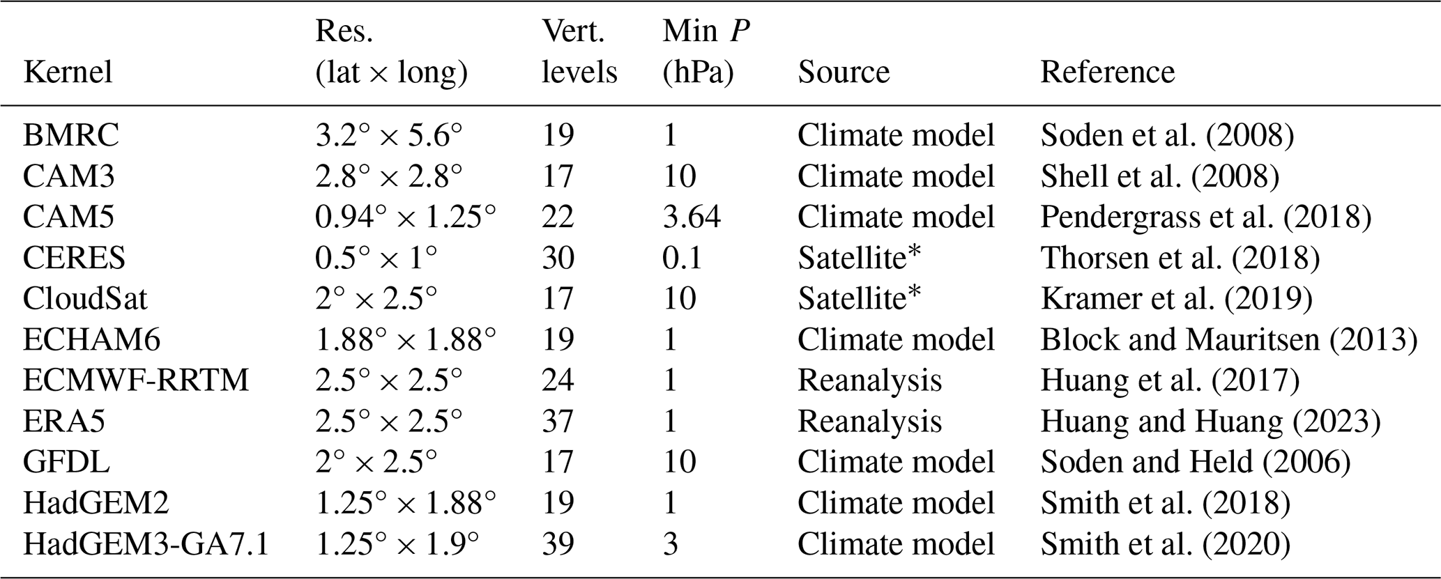
^* For kernels with a satellite data source, reanalysis data were used to supplement calculations.

After collecting and regridding the kernels, we combined each kernel set into one netCDF file per source. The native kernel variables were renamed to have a standardized set of variables, and their units or other metadata were altered for consistency and accuracy. For example, all surface albedo kernels had their units changed to W m⁻² % ⁻¹ if needed. We then inspected the kernels to find inconsistencies with their sign conventions, which were corrected. The resulting dataset was uploaded to Zenodo (Janoski et al., 2025a), which can be downloaded manually or via a built-in script in the ClimKern Python package.

2.2 Sample climate model output

We also provide a tutorial dataset within the package to calculate, for verification purposes, the feedbacks given in Table 2. The package includes a function that accesses the sample data derived from pre-industrial and abrupt-2×CO₂ fully coupled runs using the Large Ensemble version of the Community Earth System Model 1 (CESM1-LE). The CESM1-LE model incorporates the Community Atmosphere Model version 5 (CAM5) with 30 vertical levels and the Parallel Ocean Program version 2 (POP2) with 60 vertical levels. The model operates at a horizontal resolution of 1° across all components (Kay et al., 2015). These experiments have been extensively documented in prior studies (Mitevski et al., 2021, 2022, 2023). We also provide the effective radiative forcing (ERF), calculated as the difference between the global mean net TOA flux between an abrupt 2×CO₂ run and pre-industrial control run where the sea surface temperatures and sea ice concentrations are fixed to pre-industrial conditions in both runs (Forster et al., 2016).

3 Feedback calculations

The ClimKern Python package (Janoski et al., 2025b), hereafter referred to as simply “ClimKern”, contains many built-in functions for calculating radiative feedbacks and other valuable quantities of interest. Note that all outputs from feedback functions are TOA radiative perturbations from the feedback in units of W m⁻²; if the user wishes to express feedback values per unit temperature (W m⁻² K⁻¹), that can be achieved by dividing or regressing by the surface temperature response. We avoided incorporating this step into the functions as there are several ways of expressing feedbacks, such as in the form of warming contributions (Pithan and Mauritsen, 2014; Goosse et al., 2018; Previdi et al., 2020; Janoski et al., 2023), and the radiative perturbations in W m⁻² are helpful in calculating rapid adjustments to radiative forcing (Vial et al., 2013; Block and Mauritsen, 2013; Smith et al., 2018). All functions can compute all-sky and clear-sky feedbacks depending on the sky argument, either “all-sky” or “clear-sky”. Additionally, because radiative kernels are typically only available as monthly means and monthly means are standard climate model output, ClimKern currently only accepts monthly mean input fields. Below, we document the required user input for the feedback calculation functions and provide details on their methodologies. This is not an exhaustive list of functions available in ClimKern, and specifics are subject to change in future versions. Still, we hope it will prove helpful to discuss the philosophy behind the design of each function.

3.1 Temperature feedbacks

Temperature feedbacks refer to the radiative perturbations at the TOA from changes in the surface and atmospheric temperatures. Traditionally, the total temperature feedback is decomposed into the Planck feedback (or Planck response, depending on the specific definition of “feedback” used) and the lapse rate feedback (Soden and Held, 2006; Bony et al., 2006; Soden et al., 2008). The Planck feedback is the radiative response to a vertically uniform temperature change of equal magnitude to that of the surface; it is the most fundamental response of the radiative budget to a change in temperature, following the Stefan–Boltzmann law (Previdi et al., 2021). The lapse rate feedback is instead the deviation from vertically uniform warming to quantify the radiative effects of an altered tropospheric lapse rate.

ClimKern provides the calc_T_feedbacks function that computes the tropospheric Planck and lapse rate feedbacks using user-provided 4-D air temperature and 3-D surface temperature and pressure fields from two climate model simulations: a control simulation (representing a baseline state of the climate system) and a perturbed simulation (representing the climate system under changed conditions, such as increased greenhouse gas or aerosol concentrations), the difference of which is used to calculate the temperature response. In the tutorial data provided with ClimKern, these are a 1×CO₂ and a 2×CO₂ (relative to preindustrial levels) simulation, respectively. Reanalysis data can be used similarly by separating data into two time periods for comparison.

First, ClimKern checks the input to ensure its format is compatible, including checking the time dimensions and units; then, the function will either proceed, issuing a warning to the user if any assumptions are made for missing metadata or return an error for major incompatibilities (e.g., not providing input in the form of an Xarray DataArray Hoyer and Hamman, 2017). If the user did not provide an optional model- or user-defined tropopause, ClimKern will create a tropopause defined as 100 hPa at the Equator and linearly increasing with the cosine of latitude to 300 hPa at the poles. It will also read in the user-selected temperature and surface temperature kernels from locally stored package data. Using the xESMF module (Zhuang et al., 2023), the kernels are horizontally regridded using bilinear interpolation with periodic boundary conditions to match the resolution of the input model data. We elected to horizontally regrid to the input data's resolution so that the user always receives output on the same horizontal grid as the input.

Following this setup, ClimKern creates a monthly climatology from the control simulation surface and atmospheric temperatures and subtracts it from the perturbed simulation fields, yielding a surface and air temperature response. ClimKern uses the control simulation's climatological surface pressure to mask values below the surface for the air temperature response. The air temperature response is linearly interpolated to match the vertical kernel resolution; subsequent testing for tropospheric feedbacks at the TOA demonstrates little difference if the input vertical resolution is used (not shown). Layer thicknesses are then calculated for the subsequent vertical integration of the temperature feedbacks. The user-supplied perturbed simulation pressure and optional tropopause height are used when calculating the layer thicknesses to ensure that the vertical integration only extends from the surface to the tropopause.

The total air temperature response is decomposed into a vertically uniform component and deviation to calculate the Planck and lapse rate feedbacks separately. Both feedbacks are calculated by multiplying the respective temperature response component, temperature kernel, and layer thickness array and taking a sum along the pressure axis. In the case of the Planck feedback, the surface temperature response is multiplied by the surface temperature kernel and added to this sum. The function then returns both feedbacks. To the user, all of this culminates in two lines of code:

import climkern as ck
LR,Planck = ck.calc_T_
feedbacks(ctrl.T,ctrl.TS,ctrl.PS,
          pert.T,pert.TS,pert.PS,
          pert.TROP_P,kern="GFDL",
          sky="all-sky",fixRH=False),

where LR and Planck are the vertically integrated, monthly and spatially varying lapse rate and Planck feedbacks, respectively; ctrl and pert are Xarray Datasets (Hoyer and Hamman, 2017) containing the control and perturbed simulation output; T is the 4-dimensional air temperature; TS is the 3-dimensional surface temperature; PS is the 3-dimensional surface pressure; TROP_P is the optional 3-dimensional tropopause height; and kern is the optional kernel choice argument. All feedback calculations share this kern argument, which defaults to “GFDL” to specify which of the 11 kernels ClimKern should use.

This function contains several optional arguments, including the kernel name, tropopause heights, whether to calculate the all-sky or clear-sky feedbacks, and whether to use relative humidity as a state variable, as in Held and Shell (2012). Further details about the computations and optional parameters can be found in the source code in Janoski et al. (2025b).

3.2 Water vapor feedback

ClimKern also offers a calc_q_feedbacks function to compute water vapor feedbacks:

q_lw,q_sw = ck.calc_q_
feedbacks(ctrl.Q,ctrl.T,ctrl.PS,
          pert.Q,pert.PS,pert.TROP_P,
          kern="GFDL",method=1),

where q_lw and q_sw are the TOA radiative perturbations from the longwave and shortwave water vapor feedbacks, respectively; Q is the 4-dimensional specific humidity; and all other variables are as they are in Sect. 3.1. Note that a “control” air temperature variable is required because water vapor kernels are traditionally calculated not using a unit increase in specific humidity but rather the specific humidity change corresponding to a 1 K increase in temperature with constant relative humidity (Shell et al., 2008); consequently, the unit of the water vapor kernels is W m⁻² K⁻¹.

The flow of the function is similar to that of the temperature feedbacks: first, ClimKern checks all input data and tries to identify proper units. If the user did not provide a DataArray with tropopause pressure, ClimKern constructs a default one. Next, ClimKern produces a monthly climatology of the control simulation surface pressure, specific humidity, and air temperature. Like the temperature feedback function, the kernels are regridded to the horizontal grid of the input data, and the climatologies of the specific humidity, air temperature, and the specific humidity response are put on kernel pressure levels. Values on pressure levels below the control simulations's climatological surface pressure are masked and not included in further calculations. The product of the kernel, specific humidity response, and layer thickness is vertically integrated over the troposphere; a normalization factor must also be included, as discussed below.

Water vapor feedbacks are commonly computed using the change in the natural log of specific humidity because water vapor's absorption of longwave radiation is roughly proportional to the logarithm of its concentration (Shell et al., 2008; Lacis et al., 2013; Colman and Soden, 2021). The change in the natural log of specific humidity can be written as

$$\begin{array}{}\text{(4)}& \mathrm{\Delta }\ln \left(q\right)=\ln \left(q_{\mathrm{pert}}\right)-\ln \left(q_{\mathrm{ctrl}}\right),\end{array}$$

where q_pert and q_ctrl are the perturbed and control specific humidities, respectively. Using logarithm properties, this can be expressed as

$$\begin{array}{}\text{(5)}& \mathrm{\Delta }\ln \left(q\right)=\ln \left(\mathrm{1}+{\displaystyle \frac{\mathrm{\Delta }q}{q_{\mathrm{ctrl}}}}\right),\end{array}$$

where $\mathrm{\Delta }q=q_{\mathrm{pert}}-q_{\mathrm{ctrl}}$. For small changes in q such that $(\mathrm{\Delta }q/q_{\mathrm{ctrl}})\ll \mathrm{1}$, the natural logarithm can be approximated using a first-order Taylor expansion:

$$\begin{array}{}\text{(6)}& \ln \left(\mathrm{1}+{\displaystyle \frac{\mathrm{\Delta }q}{q_{\mathrm{ctrl}}}}\right)\approx {\displaystyle \frac{\mathrm{\Delta }q}{q_{\mathrm{ctrl}}}},\end{array}$$

leading to the fractional approximation used in Pendergrass (2019):

$$\begin{array}{}\text{(7)}& \mathrm{\Delta }\ln \left(q\right)\approx {\displaystyle \frac{\mathrm{\Delta }q}{q_{\mathrm{ctrl}}}}.\end{array}$$

ClimKern allows the user to choose whether to use this legacy fractional approximation or use the more precise, actual difference in natural logs of specific humidity for water vapor feedback calculations via the method parameter in the calc_q_feedbacks function, outlined below. Alternatively, users may instead use the linear change in specific humidity, i.e.,

$$\begin{array}{}\text{(8)}& \mathrm{\Delta }q=q_{\mathrm{pert}}-q_{\mathrm{ctrl}}.\end{array}$$

The water vapor kernels must be normalized by the change in specific humidity per unit temperature increase. Ideally, one would have this field from the kernel-producing simulation, as in Shell et al. (2008) and Pendergrass (2019), but, in practice, this quantity is rarely included with the distributed kernels. Given the little information available about the base states used in the individual kernel calculations, ClimKern utilizes the climatological air temperature from the user-provided control simulation to produce a water vapor kernel normalization factor using the Buck (1981) empirical formula for saturation vapor pressure. Note that the change in specific humidity per unit temperature increase can similarly either be the logarithmic or linear change and, in the case of the former, use the fractional approximation.

The calc_q_feedbacks function contains four “method” options to accommodate the variations in the literature described above. The options and corresponding numeric arguments are the following:

1. use the actual logarithm for both the specific humidity response and normalization factor

2. use the actual logarithm for the specific humidity response and fractional approximation for the normalization factor

3. use the fractional approximation in the specific humidity response and normalization factor

4. use the linear change for both the specific humidity response and normalization factor.

The function defaults to option 1. Further details can be found in the function's docstring (Janoski et al., 2025b).

3.3 Surface albedo feedback

The calc_alb_feedback function, which computes surface albedo feedback, is relatively straightforward; it requires the user to provide the upwelling and downwelling shortwave radiation at the surface from the control and perturbed simulations. The first step is to compute the surface albedo as the ratio of surface upwelling to downwelling radiation while masking areas with a downwelling radiation value of 0 W m⁻². ClimKern then takes the difference between the perturbed simulation's albedo and the control simulation's monthly climatological albedo. The desired albedo kernel is loaded from memory, regridded to the input horizontal resolution, and multiplied by the albedo response to produce the surface albedo feedback.

3.4 Cloud feedbacks

Cloud feedbacks are comparatively more complicated than the other feedbacks, owing to nonlinearities in kernel computations and the vertical overlapping of clouds (Soden and Held, 2006; Soden et al., 2008; Shell et al., 2008). Consequently, traditional kernel sets do not include explicit shortwave or longwave cloud kernels, requiring alternate methods for calculating cloud feedbacks – most commonly, the residual and adjustment methods. ClimKern contains a function for each method, which we will detail below. Note that for both methods, ClimKern optionally accepts radiative forcing terms that will vary with the experimental setup (i.e., control and perturbation simulations). In other words, there is not a precise type of radiative forcing quantity that will suit every scenario. ClimKern avoids making assumptions regarding the forcing; if the user does not provide it, cloud feedback functions assume the radiative forcing terms are zero by default. We use the ERF to compute cloud feedback in our sample results (Sect. 4).

3.4.1 Residual method

In the residual method, the cloud feedbacks are computed as a residual of the TOA energy budget:

$$\begin{array}{}\text{(9)}& \mathrm{\Delta }{R}_{\mathrm{cloud}}=\mathrm{\Delta }R-\mathrm{\Delta }F-\sum _i\mathrm{\Delta }{R}_i,\end{array}$$

where ΔR_cloud is the TOA radiative perturbation from the cloud feedback, ΔR is the all-sky net TOA radiative imbalance, ΔF is the radiative forcing (e.g., from CO₂), and ∑_iΔR_i is the sum of the TOA radiative perturbations from other non-cloud feedbacks (Soden and Held, 2006; Zhang et al., 2018; Zhu et al., 2019). Put another way, the cloud feedback is assumed to be the missing piece in the TOA radiative budget after accounting for other terms. Although this method provides a “clean” approach that fully closes the radiative budget in a kernel feedback decomposition, it carries two main drawbacks. First, it is highly sensitive to uncertainties in the other terms and the often unavailable radiative forcing, ΔF (Soden et al., 2008). Second, since the cloud feedbacks are assumed to close the radiative budget, feedback decompositions using this method yield no separate error estimate, which is sometimes valuable for evaluating radiative kernels. Despite these disadvantages, the residual method is still used.

ClimKern contains separate calc_cloud_LW_res and calc_cloud_SW_res functions to calculate the longwave and shortwave cloud feedbacks, respectively. For the longwave, ClimKern requires net longwave radiative flux at the TOA from the control and perturbed simulations, the longwave all-sky radiative forcing, and the radiative perturbations from the total temperature and longwave water vapor feedbacks. The shortwave function instead requires the net shortwave radiative flux at the TOA in the control and perturbed simulations, the shortwave all-sky radiative forcing, and the radiative perturbations from the surface albedo and shortwave water vapor feedbacks. From there, both functions compute the cloud feedback using Eq. (9).

3.4.2 Adjustment method

The adjustment method for calculating cloud feedbacks is named as such because the change in cloud radiative effect (CRE) is “adjusted” for masking by other feedbacks and the radiative forcing to produce a cloud feedback:

$$\begin{array}{}\text{(10)}& \mathrm{\Delta }{R}_{\mathrm{cloud}}=\mathrm{\Delta }\mathrm{CRE}+\sum _i(\mathrm{\Delta }{R}_i^{\mathrm{o}}-\mathrm{\Delta }{R}_i)+(\mathrm{\Delta }{F}^{\mathrm{o}}-\mathrm{\Delta }F),\end{array}$$

where ΔCRE is the CRE response, $\mathrm{\Delta }{R}_i^{\mathrm{o}}$ and ΔR_i are the clear-sky and all-sky radiative feedbacks, and ΔF^o and ΔF are the clear-sky and all-sky radiative forcings (Soden et al., 2008; Zhang et al., 2018). ΔCRE is computed as ΔR−ΔR^o, i.e., the difference in the all-sky and clear-sky TOA radiative flux. The adjustment method is considered less sensitive to uncertainties in the other terms, especially the forcing term (Soden et al., 2008). Additionally, since the resulting cloud feedback is not computed as a residual, it allows one to separately quantify the error in closing the TOA radiative budget.

The longwave and shortwave adjustment-method cloud feedbacks can be computed via the calc_cloud_LW and calc_cloud_SW functions. The longwave function accepts the change in the longwave CRE and the all-sky and clear-sky radiative perturbations at the TOA from the total temperature feedback, longwave water vapor feedback, and longwave radiative forcing. The shortwave function uses the shortwave versions of the longwave function input, except that it uses the surface albedo feedback instead of the temperature feedback. ClimKern includes separate calc_dCRE_LW and calc_dCRE_SW functions that evaluate the change in longwave and shortwave CRE and that require several radiative fields from the user, including the TOA all-sky and clear-sky LW or SW radiative fluxes in the control and perturbation simulations. After reading in all the necessary input, the adjustment method cloud feedback functions calculate the differences between the all-sky and clear-sky perturbations from non-cloud terms and combine them with the change in CRE to return the desired cloud feedback.

3.5 Other functions

We included several other utility functions in ClimKern. First, there are stratosphere versions of the temperature and water vapor feedback functions, named calc_strato_T and calc_strato_q, respectively. They are mostly analogous to their tropospheric counterparts, but the vertical integration is performed from the tropopause to the TOA. Next, ClimKern provides a calc_RH_feedback function to calculate the relative humidity feedback following Shell et al. (2008), Held and Shell (2012), and Zelinka et al. (2020). Typically, the relative humidity feedback would be a component of a radiative feedback decomposition if the user calculated the temperature feedbacks with the fixRH option. Finally, the spat_avg function computes the spatial average of a DataArray while weighting for the cosine of latitude. We refer the reader to Janoski et al. (2025b) for additional documentation.

4 Results with sample data

4.1 Radiative kernels

Having outlined the data and functions packaged with ClimKern, we now focus on the characteristics of the TOA radiative kernels. Figure 1 shows the annual- and zonal-average mean kernel values and two across-kernel standard deviation ranges after linearly interpolating to common 17 standard pressure levels. The mean and standard deviation of the all-sky air temperature kernels (Fig. 1a) have two local maxima in magnitude: one in the equatorial upper troposphere and the other in the mid- to high-latitude lower troposphere in the Southern Hemisphere (SH). In the clear-sky kernels, the lower tropospheric maximum is located over the Equator rather than the extratropical SH (Fig. 1b). Because the all-sky and clear-sky kernels differ only by the existence of cloud effects in their calculations, the different maxima locations are likely a result of clouds, which exert considerable influence on temperature kernels via cloud-top height temperatures; for example, high, cold clouds reduce outgoing longwave radiation efficiency by altering the effective emission height, affecting temperature kernel values (Kramer et al., 2019). The clear-sky air temperature kernels exhibit less spread (max ∼0.06 W m⁻² K⁻¹ 100 hPa⁻¹) than the all-sky kernels (max ∼0.13 W m⁻² K⁻¹ 100 hPa⁻¹) (Fig. 1a–b), implicating the uncertainty introduced by clouds in radiative schemes.

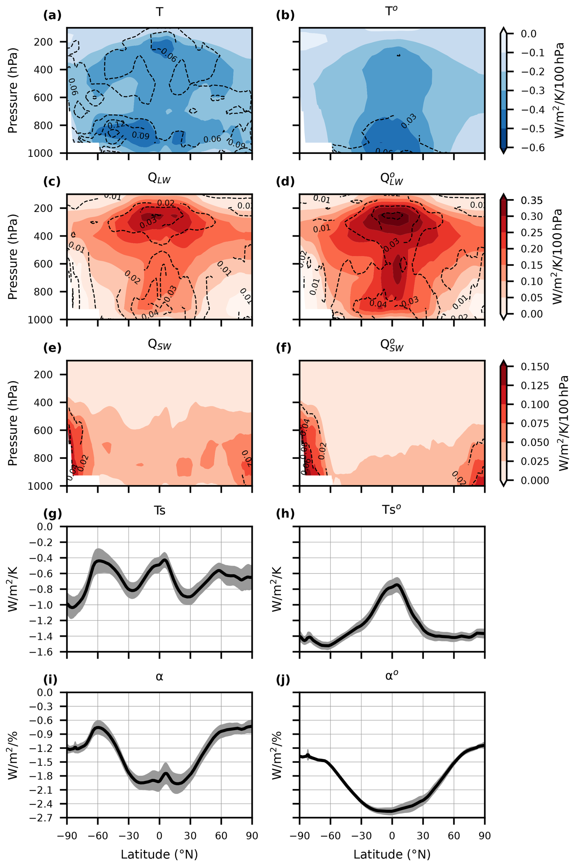
Figure 1 (a–b) The mean (shaded) and standard deviation (contoured, dashed) of the all-sky (left) and clear-sky (right) temperature kernels, representing the response to a 1 K increase in temperature. Panels (c–d) are as in (a–b) but for the longwave water vapor kernels, which reflect specific humidity changes associated with a 1 K warming and fixed relative humidity. Panels (e–f) are as in (a–b) but for the shortwave water vapor kernels. (g–h) The mean (solid line) represents ± 1 standard deviation (shading) of the all-sky (left) and clear-sky (right) surface temperature kernels. Panels (i–j) are as in (g–h) but for the surface albedo kernels, corresponding to a 1 % increase in surface albedo.

The longwave water vapor kernels (Fig. 1c–d) do not appear to show as large sensitivity to clouds as the air temperature kernels, except for the deep tropics between 800 and 400 hPa. The longwave water vapor kernel mean is largest in the equatorial upper troposphere and decreases with latitude, consistent with the findings of Huang et al. (2007). The pattern of the standard deviation mostly follows that of the mean with equatorial maxima in both the high and low troposphere (Fig. 1c–d), indicating that this region is particularly sensitive to the base state and physics used in kernel production. The shortwave water vapor kernels (Fig. 1e–f) exhibit an increase in mean and standard deviation with latitude, opposite to that of the longwave kernels. As suggested by Huang and Huang (2023), the higher shortwave reflectivity of land and ice surfaces vs. ocean surfaces likely causes this behavior. Interkernel spread in the shortwave water vapor kernel is larger near the poles, which may be due to differences in the radiative characteristics of the surface (e.g., sea ice extent, snow cover) in the kernel base states.

The surface temperature and albedo kernels are 3-dimensional, so the annual and zonal averages only vary with latitude (Fig. 1g–j). The surface temperature kernel is highly sensitive to clouds, especially in the extratropics, as evidenced by local maxima near 60° N/S in the all-sky kernels only (Fig. 1g–h). Interkernel spread is relatively constant with latitude. In the case of the all-sky surface albedo kernel (Fig. 1i–j), interkernel spread is larger in the tropics (∼0.4 W m⁻² %⁻¹) than the extratropics (∼0.2 W m⁻² %−1). The clear-sky version of the kernel exhibits the greatest variability in the Northern Hemisphere tropics (∼0.3 W m⁻² %⁻¹) and decreases with latitude. The clear-sky surface albedo interkernel spread is less than the all-sky spread at all latitudes, indicating that clouds are a main contributor to the latter. In the next section, we explore how the spatial structure of the kernel means and interkernel spread influence the resulting radiative feedbacks.

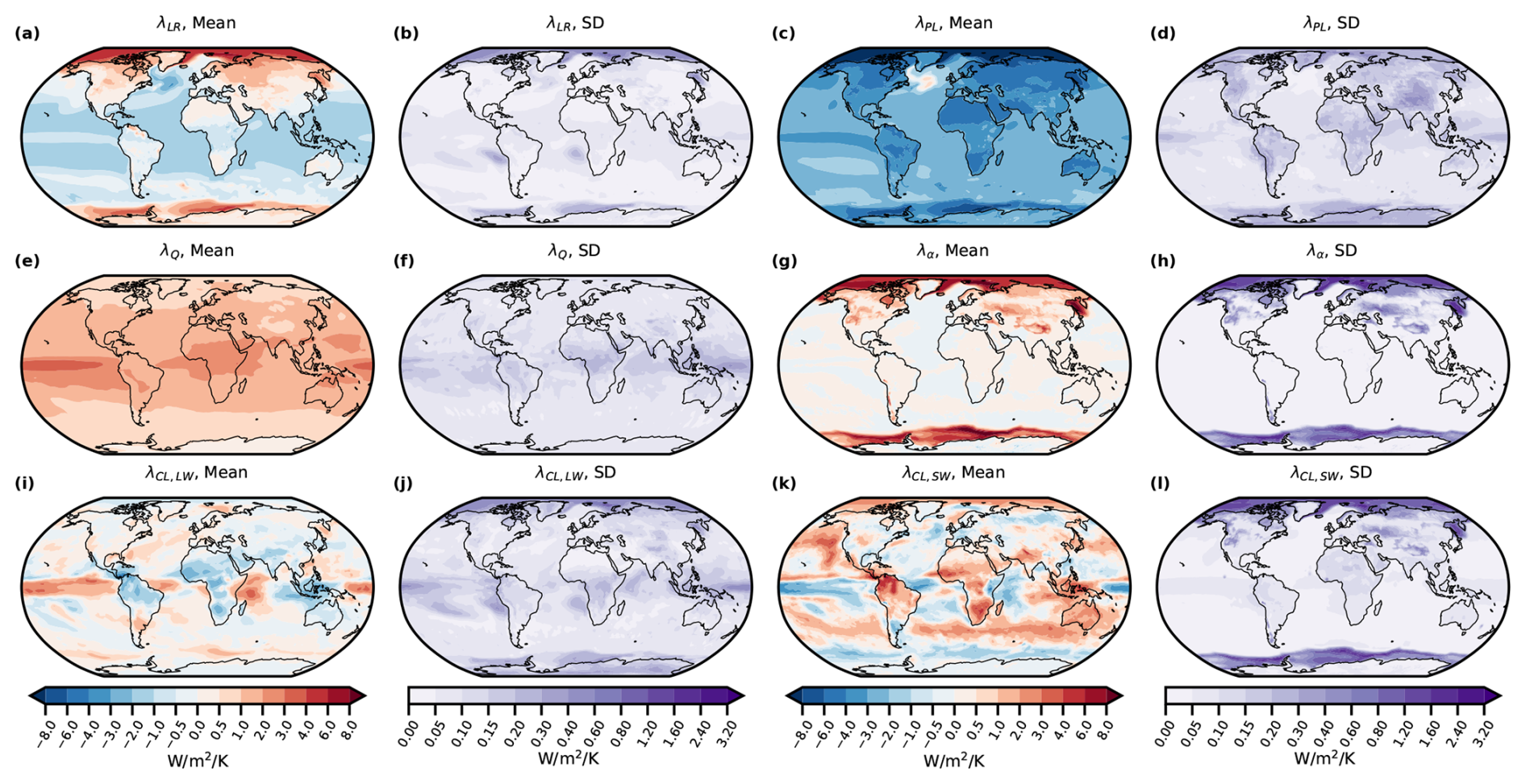
Figure 2 First and third columns from left: the annual, kernel mean (a) lapse rate, (c) Planck, (e) water vapor, (g) surface albedo, (i) longwave cloud, and (k) shortwave cloud feedbacks. Second and fourth columns: as for the first and third columns, but showing the standard deviation (SD) among kernels. Cloud feedbacks were calculated using the adjustment method. Values are expressed in units of W m⁻² K⁻¹ by normalizing by the global mean surface temperature response. Note the nonlinear color bar scales for both the means and standard deviations used to make maps comparable.

4.2 Feedback results

Having quantified the kernels themselves, we now focus on how the interkernel differences translate into differences in individual feedbacks. Recall that all feedbacks are calculated using identical methodologies between kernels and with the same CESM1-LE sample model output data described in Sect. 2.2 such that feedback variability is solely the result of the kernel choice. Feedbacks were computed using the difference in the monthly climatology of the last 30 years of the preindustrial control and a standard 150-year-long 2×CO₂ simulation. Temperature and water vapor feedbacks are vertically integrated from the surface to the model-derived tropopause in the 2×CO₂ simulation via the TROP_P function argument. Water vapor feedbacks were calculated using the method-1 option, which uses the actual change in the natural log of specific humidity in calculations, although we later show global average results with the other three methods as well. Please note that all results use a single model run from CESM1-LE to compute the climate response.

The choice of defining the response as the difference between abrupt 2×CO₂ and pre-industrial control simulations was made to minimize the sample data size distributed with ClimKern while aligning with this study's goal of highlighting interkernel spread. Additionally, this approach is commonly used, as in Pithan and Mauritsen (2014), Goosse et al. (2018), Previdi et al. (2020), and Hahn et al. (2021). A notable consequence of this choice is that feedback values presented here include rapid adjustments that occur after CO₂ increases (Zelinka et al., 2020; Hahn et al., 2021).

Figure 2 shows the kernel mean (first and third columns) and standard deviation (second and fourth columns) of the lapse rate, Planck, water vapor, surface albedo, longwave cloud, and shortwave cloud feedbacks. Generally, the lapse rate and Planck feedbacks' mean and standard deviation magnitudes are greater at the poles (Fig. 2a–d). The strong latitudinal gradient and sign change in the lapse rate feedback (Fig. 2a) are well-recognized features in climate model simulations subjected to increasing CO₂. They are products of latitudinal differences in lower- and upper-tropospheric coupling, sea ice loss, and heat transport (Manabe and Wetherald, 1975; Graversen et al., 2014; Feldl et al., 2020; Colman and Soden, 2021; Previdi et al., 2021). Similarly, the kernel mean Planck feedback is most negative over the Arctic with values less than −12 W m⁻² K⁻¹ (Fig. 2c). This is where the surface temperature increase is greatest via Arctic amplification, producing large increases in outgoing longwave radiation via the Stefan–Boltzmann law. Strongly negative Planck feedbacks of less than −8 W m⁻² K⁻¹ occur over the Southern Ocean (Fig. 2c). The spatial distribution of lapse rate and Planck feedback standard deviations imply enhanced kernel sensitivity in the Arctic and Southern Ocean (Fig. 2b, d); however, standard deviation values are small compared to some other feedbacks, including the surface albedo and cloud feedbacks.

The water vapor feedback is most positive in the tropical Pacific, with values ranging from 2 to 4 W m⁻² K⁻¹ (Fig. 2e). Here, the increase in water vapor concentration per degree of warming is greatest via the Clausius–Clapeyron relationship. Interkernel spread is also maximized in the tropics but exhibits a different longitudinal distribution, with the greatest variability located over the West Pacific (Fig. 2f). The maximum in standard deviation in the West Pacific extends along the Equator and to the southeast, indicating that this feature may be related to the double Intertropical Convergence Zone (ITCZ) bias present in many climate models (Lin, 2007; Tian and Dong, 2020). As with the temperature feedbacks, interkernel spread is small (SD < 0.3 W m⁻² K⁻¹) relative to the feedbacks discussed next.

The surface albedo feedback is largest over high-latitude oceans (Fig. 2g–h), driven by sea ice loss (Curry et al., 1995; Riihelä et al., 2021). This sea ice loss leads to large bottom-heavy warming in these regions, resulting in a strong positive lapse rate feedback, negative Planck feedback, and similarity in the spatial patterns of the lapse rate, Planck, and surface albedo feedbacks (Croll, 1875; Ingram et al., 1989; Previdi et al., 2021). It is important to note that in the Arctic and Southern Ocean, the standard deviation of the surface albedo feedback is larger than that of the lapse rate, Planck, and water vapor feedbacks, with values nearly as much as 50 % of the kernel mean. Considering the difference in spread between the all-sky vs. the clear-sky albedo kernels (Fig. 1i–j), clouds likely play a role in the polar-amplified spread in albedo feedback.

The last two feedbacks we consider are the longwave and shortwave cloud feedbacks in Fig. 2i–l. The kernel mean longwave cloud feedback shows spatial inhomogeneity with maxima in the tropical Pacific and western Indian oceans and minima over northern South America, Africa, and Indonesia (Fig. 2i). The standard deviation of the longwave cloud feedback tends to increase poleward aside from relatively large values (∼0.4 W m⁻² K⁻¹) in the equatorial Pacific (Fig. 2j). Considerable spatial inhomogeneity is also found in the kernel mean shortwave cloud feedback, ranging from −4 W m⁻² K⁻¹ in the western equatorial Pacific to 7 W m⁻² K⁻¹ in northern South America (Fig. 2k). The shortwave cloud feedback standard deviation is largest over the Arctic and Southern Ocean (Fig. 2l). The highest standard deviation values among all feedbacks are those of the surface albedo and shortwave cloud feedbacks in these regions, highlighting the importance of kernel choice near the poles.

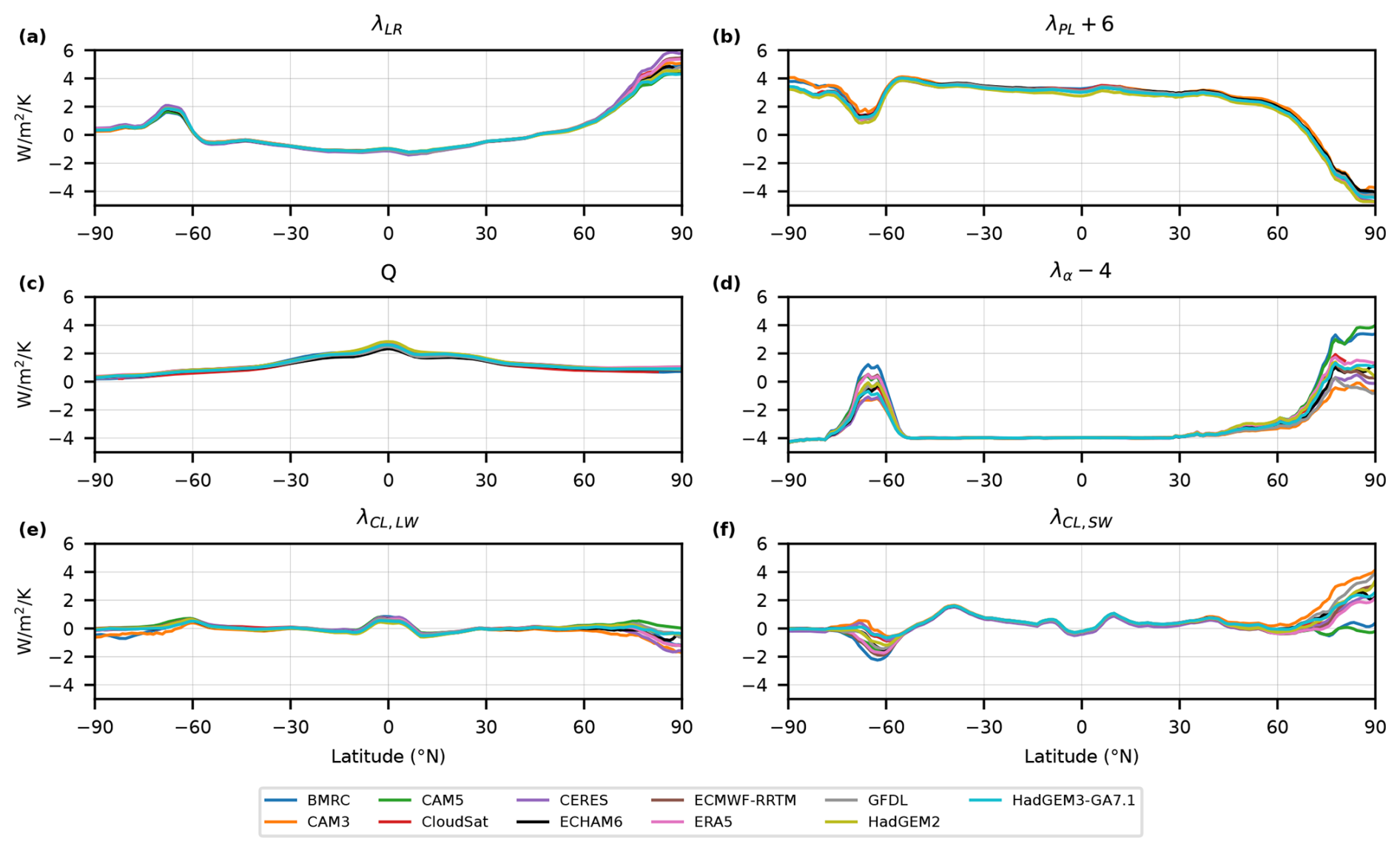
Figure 3 Annual zonal mean (a) lapse rate, (b) Planck, (c) total water vapor, (d) surface albedo, (e) longwave cloud, and (f) shortwave cloud feedbacks calculated using the adjustment method for each of the 11 kernels included in ClimKern in W m⁻² K⁻¹; 6 W m⁻² K⁻¹ is added to the Planck feedback, and 4 W m⁻² K⁻¹ is subtracted from the surface albedo feedback for visualization and comparison purposes.

Having analyzed the spatial distribution of interkernel spread, we focus on the differences between individual kernels in the zonal mean feedbacks in Fig. 3. The lapse rate and Planck feedbacks show minimal spread throughout the tropics and midlatitudes, with the greatest spread in the Arctic (Fig. 3a–b). The lapse rate feedback varies between 4 and 6 W m⁻² K⁻¹ poleward of 80° N but varies by less than 1 W m⁻² K⁻¹ elsewhere (Fig. 3a). For the Planck feedback, interkernel spread is greatest poleward of 80° but generally less than 1 W m⁻² K⁻¹ everywhere (Fig. 3b). The zonal mean water vapor feedback shows little sensitivity to kernel choice but is most sensitive in the tropics with a spread of ∼0.5 W m⁻² K⁻¹ (Fig. 3c), similar to the spatial map (Fig. 2f).

Interkernel spread in the surface albedo feedback is large relative to the kernel mean, especially in the Arctic. The area-average interkernel spread north of 70° N is 2.8 W m⁻² K⁻¹, roughly two-thirds of the kernel mean surface albedo feedback for the same region (4.2 W m⁻² K⁻¹). There is a similar, albeit weaker, interkernel spread in the surface albedo feedback in the Southern Ocean. These features are particularly important in polar amplification studies, which we discuss in Sect. 5.

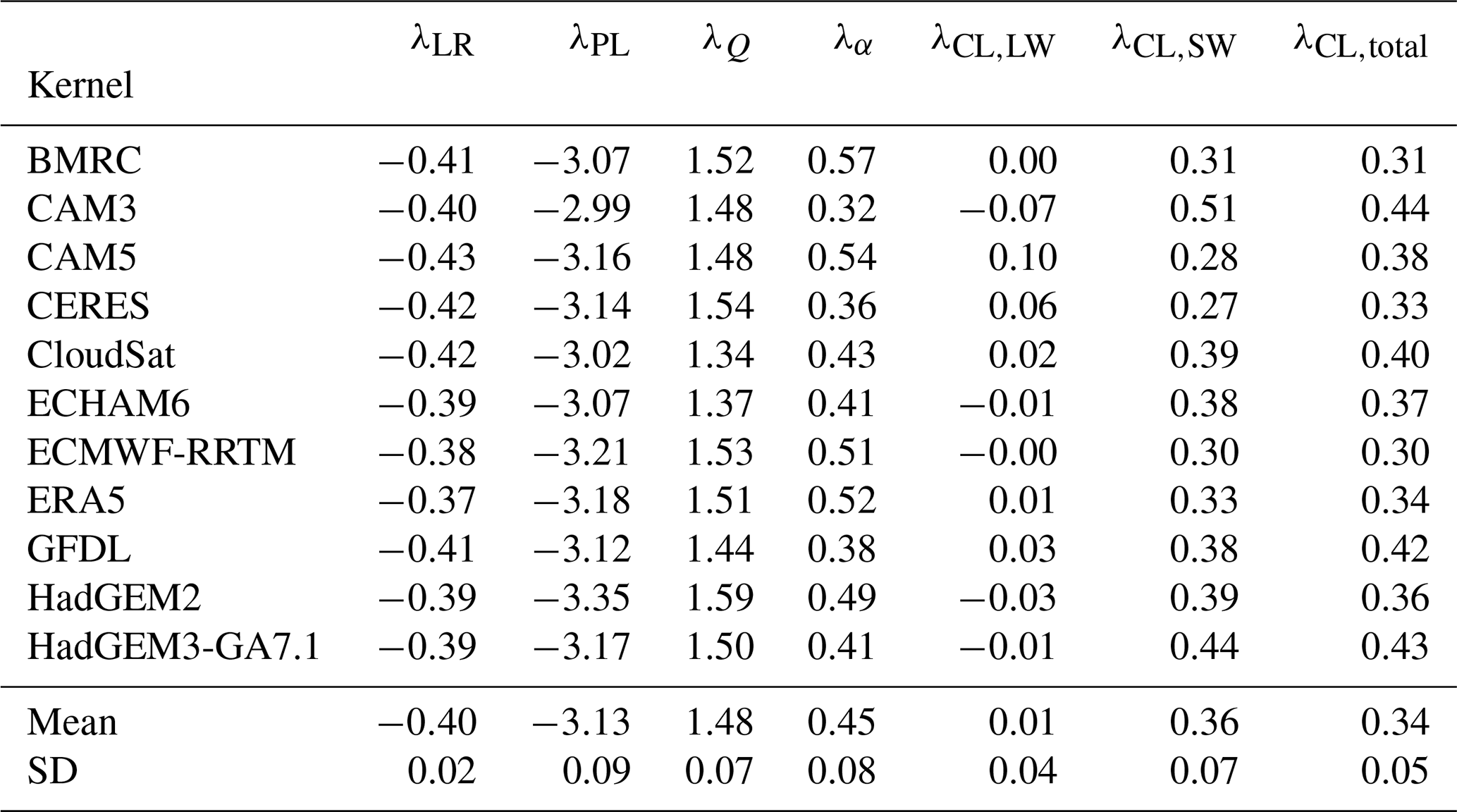
Table 2 The global annual mean feedback values (in W m⁻² K⁻¹), calculated using each kernel and the same sample CESM1-LE data. From left to right, they are the lapse rate, Planck, total (longwave + shortwave) water vapor, surface albedo, longwave cloud, shortwave cloud, and total cloud feedbacks. The cloud feedbacks are calculated using the adjustment method. The last two rows contain the kernel mean and standard deviation of the feedbacks.

The cloud feedbacks are particularly sensitive to kernel choice because they are prone to uncertainties in the other feedback and radiative forcing terms, even when using the adjustment method (Soden et al., 2008). The interkernel spread in the zonal mean longwave cloud feedback is largest at the poles such that its sign in the Arctic depends on kernel choice (Fig. 3e). The shortwave cloud feedback (Fig. 3f) is similarly most sensitive to kernel choice in the high latitudes, with a zonal distribution of variability similar to that of the surface albedo feedback. This is not a coincidence: the surface albedo feedback is used to calculate the shortwave cloud feedback via the adjustment method, so a large spread in the former translates to a large spread in the latter.

How do these zonal-average variations manifest in the global mean? We include the global, annual mean feedback values for all 11 kernels in Table 2, along with the multi-kernel mean and standard deviation. While the lapse rate and Planck feedbacks are consistently negative and the water vapor, surface albedo, and shortwave cloud feedbacks are consistently positive, the sign of the longwave cloud feedback is kernel-dependent, with values ranging from −0.07 to 0.10 W m⁻² K⁻¹. Interkernel variability, as gathered from the standard deviation, is greatest in the Planck feedback, followed by the surface albedo, water vapor, and shortwave cloud feedbacks (Table 2).

It is worth comparing how global, annual mean water vapor feedback values depend on the calculation method, as outlined in Sect. 3.2. Table S1 shows the global annual mean all-sky water vapor feedbacks for each kernel and method. Method 3 (fractional approximation for the specific humidity response and normalization factor) yields the greatest water vapor feedback values for all kernels, followed by methods 4, 1, and 2. This occurs because the fractional approximation systematically overestimates the change in natural logarithms for large perturbations such as 2×CO₂, while the linear change ignores the damping by the logarithm entirely. The range in kernel–mean water vapor feedback values introduced by method choice is 0.26 W m⁻² K⁻¹, with kernel mean values ranging from 1.41 to 1.67 W m⁻² K⁻¹.

Following this finding, a natural question is whether a particular kernel set does a better job at closing the radiative budget than others. This study only uses two simulations from one model for sample data and is, thus, ill-equipped to answer this question more generally; however, we may use clear-sky linearity tests to identify which kernel best closes the budget in this particular CESM1 experiment, as in Shell et al. (2008). Consider the clear-sky radiative budget at some point in time after 2×CO₂:

$$\begin{array}{}\text{(11)}& \mathrm{\Delta }{R}^{\mathrm{o}}=\mathrm{\Delta }{F}^{\mathrm{o}}+{\mathit{\lambda }}^{\mathrm{o}}\mathrm{\Delta }T+\mathrm{Re},\end{array}$$

where ΔR^o is the clear-sky TOA radiative imbalance; ΔF^o is the clear-sky 2×CO₂ ERF; λ^o is the clear-sky total feedback parameter; and Re is the residual term accounting for feedback nonlinearities, kernel errors, etc. All terms are global annual means. Kernel sets that produce the smallest-magnitude Re values do the best job closing the clear-sky radiative budget. Table S2 lists the residual values for all 11 kernel sets and 4 water vapor feedback calculation methods. The best-performing kernel set depends heavily on the water vapor feedback calculation method; for example, the Bureau of Meteorology Research Centre (BMRC) kernel set does the best job of closing the radiative budget using water vapor feedback method 1 (no fractional approximation) with a residual of −0.01 W m⁻² K⁻¹, but it is the second-to-last kernel set in terms of budget closure when using method 3 (with fractional approximation) with a residual of −0.25 W m⁻² K⁻¹ (Table S2). Focusing only on the first method, which is the most physically sound and uses the fewest assumptions, both CAM3 and CAM5 kernel sets perform well and are the second and fourth best at closing the clear-sky radiative budget, respectively. This result is, perhaps, unsurprising given that CAM5 is the atmosphere model included in CESM1, and CAM3 is an earlier version of CAM5. We avoid making claims regarding these kernel sets' performance when applied to other models and simulations and simply assert that kernel choice is potentially important for accurately decomposing a model simulation's radiative budget.

5 Conclusions

The radiative kernel method is a popular and efficient way of diagnosing radiative feedbacks in climate model simulations. We were motivated to develop ClimKern to streamline these sometimes complicated calculations, shed light on kernel choice's importance in feedback studies, and provide access to a growing collection of existing kernels. We used ClimKern to compute basic radiative feedbacks from a sample climate model output to quantify kernel differences, leading us to the following conclusions.

ClimKern makes radiative feedback calculations with kernels considerably easier while standardizing the underlying assumptions and methods. The ClimKern Python package contains straightforward, one-line commands for the most common calculations required for computing radiative feedbacks and can automatically load in data from the ClimKern data repository. The code is well-documented and easily accessible on GitHub and the Python Package Index for full transparency. Operations like vertical integration or horizontal regridding are consistent across the functions, even while offering the user different options. The repository similarly employs standard and consistent nomenclature across all kernels, making it a practical resource for anyone wishing to compute radiative feedbacks.

Kernel choice is a non-negligible source of uncertainty in radiative feedback calculations, especially in the polar regions. In terms of global average feedbacks, the lapse rate feedback appears to be the least sensitive to kernel choice. In contrast, the surface albedo and cloud feedbacks show considerably more sensitivity to the choice of kernel (Table 2). Interkernel spread is horizontally and vertically inhomogeneous, with all but the water vapor feedback showing the greatest kernel sensitivity at the poles (Fig. 2); spread may be a result of either differences in the base states or radiative schemes used to produce the radiative kernels. The spread in the clear-sky temperature and surface albedo kernels is smaller than their all-sky counterparts, suggesting that clouds are an important source of interkernel variability.

Polar amplification studies frequently use the radiative kernel method to compare surface warming contributions at the poles to the global or tropical average and then rank the relative importance of the individual feedbacks (Pithan and Mauritsen, 2014; Stuecker et al., 2018; Previdi et al., 2020; Hahn et al., 2021; Janoski et al., 2023). Two of the feedbacks most often identified as dominant polar amplification contributors, the lapse rate and surface albedo feedbacks (Pithan and Mauritsen, 2014; Goosse et al., 2018; Previdi et al., 2020, 2021; Hahn et al., 2021), exhibit maximum interkernel variability in the Arctic (Fig. 2), further complicating comparisons between studies that use different radiative kernels.

Kernel choice can impact climate sensitivity studies that use global mean values. The mean Planck and surface albedo feedbacks show the greatest interkernel variability, while the sign of the mean longwave cloud feedback is kernel-dependent in this single CESM1 experiment. Although it is unclear how the variability introduced by kernel choice compares to that of other methodological choices, e.g., model or forcing scenario, it highlights its impact across spatial scales, leading to our final point.

Future studies invoking the calculations of climate feedbacks can be more robust if they include a discussion of the sensitivity of the results to kernel choice. One option would be to use multiple kernels from the ClimKern repository in a sensitivity analysis to explore this. Another option would be to take the kernel average of feedbacks instead of relying on individual kernels. Although a kernel average may dilute the benefits of using more advanced or better-performing kernels, it may reduce the sensitivity to individual kernel biases. This choice may be especially appropriate in studies using multimodel ensembles to avoid relying on a single kernel that may or may not align well with all models. Future work will include comparing the sensitivity to kernel choice to other sources of uncertainty in climate studies and evaluating kernel mean performance compared to individual kernels in the computation of radiative feedbacks.

We intend for ClimKern to become a community-wide project and invite potential collaborators to contribute. The easiest way is to visit the ClimKern GitHub and fork the repository. New features and bug fixes can also be requested there.