Parameterization toolbox for a physical–biogeochemical model compatible with FABM – a case study: the coupled 1D GOTM–ECOSMO E2E for the Sylt–Rømø Bight, North Sea

Mathematical models are an invaluable tool for understanding marine ecosystems. The performance of these models is often highly dependent on their parameters. Traditionally, refining these models has involved a time-consuming trial-and-error approach to identify model parameter values that are able to reproduce observations well. However, as ecosystem models become more complex, this approach becomes impractical. With advances in computing power, optimization techniques have emerged as a viable alternative. Nevertheless, these techniques often exhibit model-specific customization, which limits their broader application. In this study, we present a parameterization toolbox based on the particle swarm optimization (PSO) algorithm, implemented within the Framework for Aquatic Biogeochemical Models (FABM). This implementation encapsulates the optimizer – that is, the toolbox itself – as a reusable component, enabling its integration across multiple models within the framework and thus making it more accessible to the community. The effectiveness of the PSO toolbox is showcased through its application in a 1D physical–biogeochemical model (GOTM–ECOSMO E2E), which successfully parameterized the Sylt–Rømø Bight ecosystem. The toolbox was able to define optimal values for most of the tuned parameters and to suggest potential ranges for poorly constrained parameters. In addition, the toolbox uncovers a number of parameter sets with notable differences in some parameter values but leading to only minor variations in biomass and fluxes. Furthermore, by experimenting with optimization models of varying complexity, the toolbox was able to define an optimal model for the Sylt–Rømø Bight.

1 Introduction

Marine biogeochemical models are valuable tools for hypothesis generation and the acquisition of a mechanistic understanding of ecosystem functioning. This understanding is particularly important given the impacts of anthropogenic-driven climate change and the increasing need to implement policies and technologies for effective mitigation. To achieve a comprehensive understanding of ecosystem functioning, it is essential to use models that are capable of reproducing the processes relevant to the system as closely as possible to observed data and real-world phenomena. However, obtaining such optimized models is challenging due to the complexity of the marine ecosystem. Firstly, unlike atmospheric and hydrodynamic models, which are based on well-established physical laws such as the Navier–Stokes equations, the governing equations for marine biogeochemical models remain incomplete (Fennel et al., 2001; Jones et al., 2010; Schartau et al., 2017). Secondly, the sparse nature of the available data often makes it difficult to constrain all model parameters (Schartau et al., 2017). Thirdly, to cover the full extent of the marine ecosystem, a number of simplifications (e.g., the use of plankton functional types) are required to reduce complexity and computational effort. As a result, processes in marine biogeochemical models are highly dependent on parameterization, which in the best case is often based on empirical studies (Miller, 2009). However, laboratory experiments to define parameters are typically conducted in a single species under controlled conditions, raising questions about their applicability to in situ conditions (Fennel et al., 2001). Where direct empirical determination is not possible, parameter optimization has been proposed to overcome these challenges (Fennel et al., 2001; Dowd, 2011). Although this approach can help models reproduce observed state variables and fluxes, its broader purpose is to systematically improve model skill by finding parameter sets that improve the agreement between model outputs and observations.

Parameter optimization has been used in marine ecosystem modeling to optimize poorly known model parameters (Prieß et al., 2013; Falls et al., 2022; Kern et al., 2024). Essentially, optimization is done by fitting the model output to the observed data through objective tuning of the parameters. The parameters are varied until the mismatch between the model outputs and the observed data, often referred to as the cost function, is minimized (Fennel et al., 2001). A variety of optimization methods used in marine ecosystem modeling (e.g., generalized likelihood uncertainty estimation – GLUE, Beven and Binley, 1992; simulated annealing – SA, Kirkpatrick et al., 1983; Markov chain Monte Carlo, Metropolis et al., 1953) have been summarized in Houska (2017). Numerous studies have succeeded in implementing parameterization and its advanced method in marine ecosystem modeling (e.g., Rückelt et al., 2009; Prieß et al., 2011; Reimer, 2019). However, these implementations are often tailored to specific models or difficult to reuse, requiring much effort to implement a new parameterization (Hemmings et al., 2015).

In biogeochemical modeling, the Framework for Aquatic Biogeochemical Models (FABM) is widely used to couple several physical and ecological models. Many important hydrodynamic and biogeochemical models are coupled to FABM (e.g., hydrodynamic models include GOTM, ROMS, NEMO, MOM, HYCOM, FVCOM, and SCHISM; ecosystem models include ECOSMO, ERSEM, BFM, PISCES – marine, and WET/PCLake – freshwater). An optimization method that is compatible with FABM would enable its use and promote its practice within the community. Therefore, in this paper, we present a parameterization toolbox that is compatible with FABM and also introduce an optimization algorithm (particle swarm optimization, PSO) that is not often used in biogeochemical models.

We demonstrate the application of the PSO to 1D GOTM–ECOSMO/ECOSMO E2E in FABM to optimize the model for the Sylt–Rømø Bight ecosystem (hereafter the Sylt ecosystem) using observational data at the Sylt Road. We chose the Sylt ecosystem as an application because there are several hypotheses about the dynamics of the Sylt ecosystem, such as (i) warmer winters leading to shifts from a pelagic to a more benthic-dominated food web, (ii) enhanced top-down control during warm winters by predators (e.g., blue mussels, oysters, razor clams) (Johannes Rick and Sabine Horn, personal communication, 2021), and (iii) bare mussel beds and mussel cultures reducing the standing stock of phytoplankton but also promoting phytoplankton primary production (Asmus and Asmus, 1991), which requires a modeling approach to address.

The structure of the paper is as follows: in the next section we describe the PSO algorithm, the cost function used in the optimization, and the coupled 1D GOTM–ECOSMO and ECOSMO E2E model configuration and setup. In the third section, we present the results and discussion of the PSO for the Sylt ecosystem. Finally we end the paper with some concluding remarks.

2 Data and methods

2.1 Parameterization toolbox

The core of the paper is the implementation of the particle swarm optimization (PSO) with FABM as the PSO toolbox. The PSO algorithm has been described well by Poli et al. (2007) and consequently well reviewed by (Garcia-Gonzalo and Fernandez-Martinez, 2012) and (Sengupta et al., 2019). The PSO from Poli et al. (2007) with a boundary condition adjustment was used to identify parameters of an ecosystem model in Puget Sound (Nguyen, 2021). The PSO toolbox presented in this paper is based on the algorithm described in Nguyen (2021). A brief description of the PSO in plain language is given below; a full description can be found in Nguyen (2021).

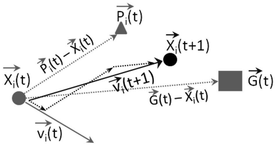
Figure 1 Particle swarm optimization algorithm. A particle i of the swarm at time t is characterized by its vector position $\overrightarrow{X_i}\left(t\right)$, its vector velocity $\overrightarrow{v_i}\left(t\right)$, and its personal cost $\overrightarrow{P_i}\left(t\right)$. The swarm at time t records its best (global) cost $\overrightarrow{G}\left(t\right)$. The particle i approaches the global best by first moving parallel to its current velocity vector ($\overrightarrow{v_i}\left(t\right)$), then parallel to the vector connecting its current position ($\overrightarrow{X_i}\left(t\right)$) to its personal best ($\overrightarrow{P_i}\left(t\right)$), and finally parallel to the vector connecting the current position ($\overrightarrow{X_i}\left(t\right)$) to the global best ($\overrightarrow{G}\left(t\right)$). The addition of these three vectors from the beginning of the first vector to the end of the third vector is its new velocity ($\overrightarrow{V_i}(t+\mathrm{1})$).

Algorithm

Mathematically, the algorithm is presented as in Fig. 1. A particle i of the swarm at time t is characterized by its vector position $\overrightarrow{X_i}\left(t\right)$, its vector velocity $\overrightarrow{v_i}\left(t\right)$, and its personal cost, $\overrightarrow{P_i}\left(t\right)$. The swarm at time t records its best (global) cost $\overrightarrow{G}\left(t\right)$. The movement of particle i from time t to time (t+1) with velocity $\overrightarrow{V_i}(t+\mathrm{1})$ must take into account its current vector velocity, its personal cost and the global (swarm) cost to reach position $\overrightarrow{X_i}(t+\mathrm{1})$ that is closer to the swarm's best position. Thus, the particle i moves first parallel to its current velocity vector ($\overrightarrow{v_i}\left(t\right)$), then parallel to the vector connecting its current position ($\overrightarrow{X_i}\left(t\right)$) to its personal best position ($\overrightarrow{P_i}\left(t\right)$), and finally parallel to the vector connecting the current position ($\overrightarrow{X_i}\left(t\right)$) to the global best position ($\overrightarrow{G}\left(t\right)$). The addition of these three vectors from the beginning of the first vector to the end of the third vector is its new velocity ($\overrightarrow{V_i}(t+\mathrm{1})$). Since the new position of particle i is determined using the previous experience of the particle itself and of the whole swarm, the new position is considered to be the better position for particle i to be in. If each particle in the swarm follows these rules, they will cooperate to find the best position in the search space and thus the best possible solution. The algorithm is implemented as follows.

1. Initialize a population array of particles with random positions and velocities on D dimensions in the search space rescaled to the interval (0, 1). The personal costs of the particles, calculated from the initialized positions and velocities, are assigned to their pbest.

2. Loop

3. For each particle, evaluate the desired optimization fitness function in D variables.

4. Compare the fitness evaluation of the particle with its pbest_i. If the current value is better than pbest_i, then set pbest_i equal to the current value and p_i equal to the current position x_i in D-dimensional space.

5. Identify the particle in the population with the best success so far, and assign its index to the global variable p_g.

6. Change the velocity and position of the particle according to the following equation (see notes below):

   $$\begin{array}{}\text{(1)}& \left\{\begin{array}{l}{\mathit{v}}_{\mathit{i}}\leftarrow \mathit{\chi }({\mathit{v}}_{\mathit{i}}+\mathit{U}(\mathrm{0},{\mathit{\varphi }}_{\mathrm{1}})\otimes ({\mathit{p}}_{\mathit{i}}-{\mathit{x}}_{\mathit{i}})+\mathit{U}(\mathrm{0},{\mathit{\varphi }}_{\mathrm{2}})\\ \otimes ({\mathit{p}}_{\mathbf{g}}-{\mathit{x}}_{\mathit{i}})),\\ {\mathit{x}}_{\mathit{i}}\leftarrow {\mathit{x}}_{\mathit{i}}+{\mathit{v}}_{\mathit{i}},\end{array}\right.\end{array}$$

   where the following applies.

   • χ represents “constriction coefficients” to control the convergence of the particle,

     $$\begin{array}{}\text{(2)}& \mathit{\chi }={\displaystyle \frac{\mathrm{2}}{\mathit{\varphi }-\mathrm{2}+\sqrt{{\mathit{\varphi }}^{\mathrm{2}}-\mathrm{4}\mathit{\varphi }}}},\end{array}$$

     where $\mathit{\varphi }={\mathit{\varphi }}_{\mathrm{1}}+{\mathit{\varphi }}_{\mathrm{2}}>\mathrm{4}$. ϕ is commonly set to 4.1, and ϕ₁=ϕ₂. ϕ₁ and ϕ₂ are often referred to as the acceleration coefficients, which determine the magnitude of the random forces in the direction of the personal best (pbest) and the global best (g).

   • U(0,ϕ_i) is a vector of random numbers uniformly distributed in [0,ϕ_i] generated randomly at each iteration and for each particle.

   • ⊗ is a component-wise multiplication.

   • Each component of v_i is kept within the range $[-V_{\text{max}},+V_{\text{max}}]$ so that particles do not go out of their search spaces. The optimal value of V_max is problem-specific, but no reasonable rule of thumb is known. For this study, V_max is half of the maximum of the search space, or 0.5.

7. If the v(x+1) potentially places x(t+1) outside its defined search space, the out-of-bounds particle must be carefully repositioned. Imagine a ball (a particle) moving with velocity v between two walls (search space). If the ball hits one of the walls, it will bounce back to a position between the two walls. To represent this, set the “damping” value, which controls the energy loss of the bouncing ball, to be something like $\mathrm{0}<\mathit{\beta }=\mathrm{0.8}<\mathrm{1}$ (quite close to 1). If the particle crosses the lower bound, then the particle is repositioned as $x(t+\mathrm{1})=r\cdot \mathit{\beta }\cdot x\left(t\right)$, where r is a random number uniformly distributed between 0 and 1. So the particle has been randomly repositioned somewhere between its original position and the lower bound (but the damping ensures that it does not get too close to its original position). If the particle crosses the upper bound, then the same bouncing ball analogy applies, but the repositioning is $x(t+\mathrm{1})=\mathrm{1}+r\cdot \mathit{\beta }\cdot \left(x\right(t)-\mathrm{1})$. (Note that this assumes that the parameter search space has been rescaled to the interval (0, 1)). The velocity of an out-of-bounds particle should also be reset. The reset velocity vector should point away from the boundary, towards the original position x(t). Sticking with the bouncing ball analogy, the velocity decreases with the distance bounced from the ground. So if the new position x(t+1) is far from the boundary, the velocity will be small. So the velocities can be rewritten as $v(t+\mathrm{1})=(r\cdot \mathit{\beta }-\mathrm{1})\cdot v\left(t\right)$, which works for particles that cross either the upper or lower boundary.

8. When a criterion is met (usually a sufficiently good fitness or a maximum number of iterations), exit the loop.

9. End

A common drawback of parameter optimization techniques is that they get trapped in a local minimum. To avoid this, the particles in the population are periodically perturbed after a predefined number of iterations, allowing them to escape the current local minimum. This perturbation is achieved by resetting the particles to high velocities, allowing them to jump far from their current positions.

The optimization fitness function. In this study, we use the Willmott skill score (WSS) (Willmott, 1981) mean absolute error (WSS_MAE, Eq. 3) (Willmott et al., 2012) to evaluate the goodness of fit of the model to the data in the PSO. WSS_MAE ranges from 0–1, with values close to 1 indicating close agreement between model predictions and observations.

$$\begin{array}{}\text{(3)}& \begin{array}{rl}{\displaystyle }\mathit{\text{WSS\_MAE}}=& {\displaystyle }\mathrm{1}-{\displaystyle \frac{\frac{\mathrm{1}}{N}{\sum }_{i=\mathrm{1}}^{i=N}|m_i-o_i|}{\frac{\mathrm{1}}{N}{\sum }_{i=\mathrm{1}}^{i=N}\left(\right|m_i-\stackrel{\mathrm{‾}}{o}|+|o_i-\stackrel{\mathrm{‾}}{o}\left|\right)}}\\ {\displaystyle }=& {\displaystyle }\mathrm{1}-{\displaystyle \frac{\mathit{\text{MAE}}}{\frac{\mathrm{1}}{N}{\sum }_{i=\mathrm{1}}^{i=N}\left(\right|m_i-\stackrel{\mathrm{‾}}{o}|+|o_i-\stackrel{\mathrm{‾}}{o}\left|\right)}}\end{array}\end{array}$$

Here, m is the model output, o is the observation, N is the number of model–observation pairs, and $\stackrel{\mathrm{‾}}{o}$ is the averaged observations.

PSO with FABM. The implementation of PSO with FABM is shown in Fig. 2.

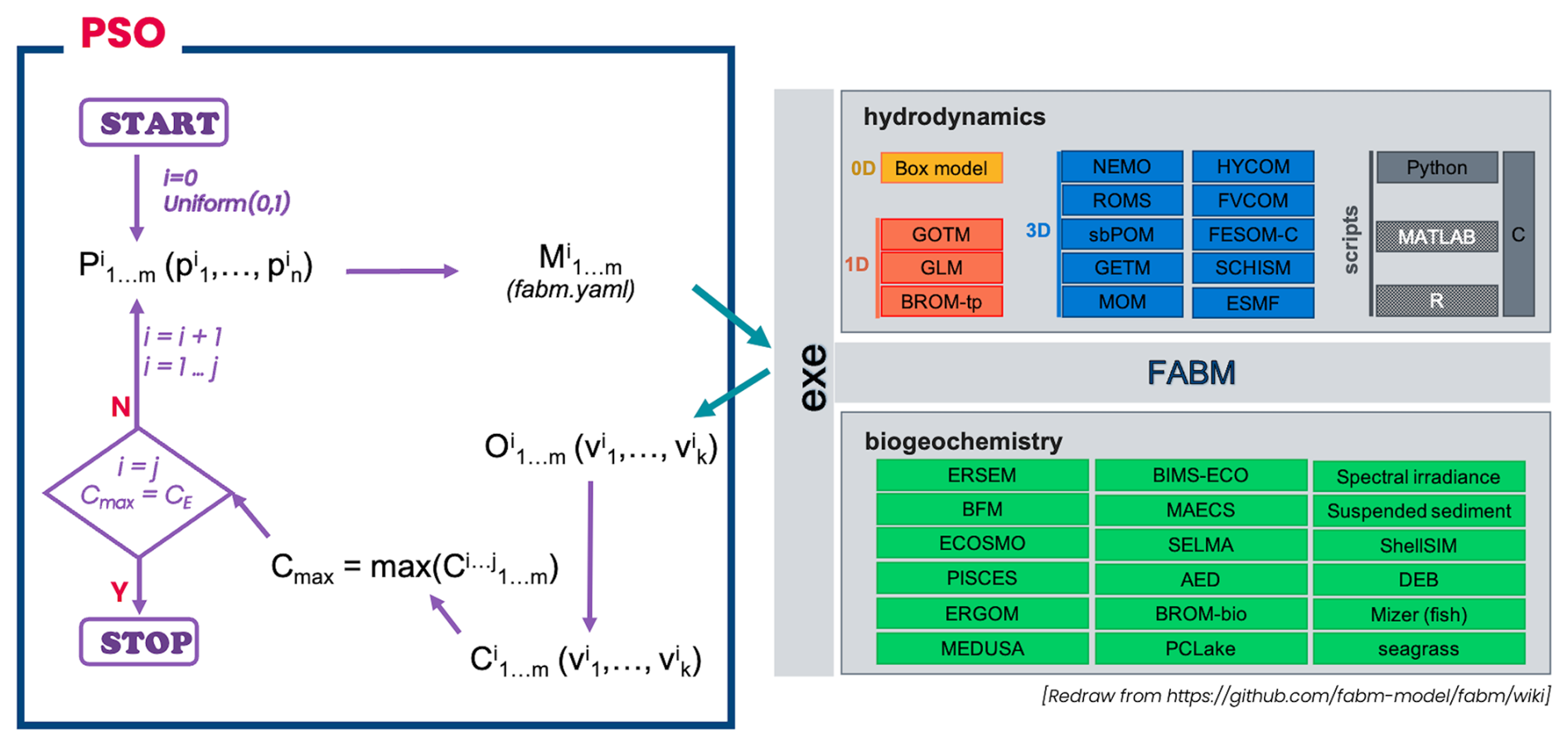
Figure 2 Implementation of the particle swarm optimization (PSO) with FABM. First, the PSO toolbox initializes a set of model evaluations ($M_{\mathrm{1},\mathrm{\dots },m}^i$) by randomly assigning parameters ($P_{\mathrm{1},\mathrm{\dots },m}^i$) for each model evaluation in the set (iteration i=0). The parameter values are restricted to the range [0, 1]. These parameters are then rescaled to their true ranges before being written to the model's fabm.yaml file. The toolbox then calls the executable file of the corresponding model or coupled model from FABM (for this study, GOTM–ECOSMO was used for demonstration) to run the model setup M. Upon completion of the model runs, the toolbox extracts the model outputs of the state variables corresponding to the observations ($O_{\mathrm{1},\mathrm{\dots },m}^i(v_{\mathrm{1}}^i,\mathrm{\dots },v_k^i)$). It then calls the cost function to compute the skill score for each state variable ($C_{\mathrm{1},\mathrm{\dots },m}^i(v_{\mathrm{1}}^i,\mathrm{\dots },v_k^i)$), identifying the maximum skill score (C_max) among all model evaluations in the set. The C_max and its corresponding parameters represent the model that best fits the observations for that iteration. The C_max and its corresponding parameters are then used as a reference point to calculate parameters for the set of model scores ($M_{\mathrm{1},\mathrm{\dots },m}^i$) in the next iteration. This process is repeated until the expected skill score (C_E) or the maximum number of iterations is reached.

The use of the toolbox requires the input of several parameters. For example, it is necessary to specify the parameters to be calibrated with their respective ranges, the directory path to the executable file of a biogeochemical (BGC) model compiled in the Framework for Aquatic Biogeochemical Models (FABM), and the evaluated state variables and corresponding observations for the calculation of model skill scores. In addition, the users must specify the number of iterations to run the PSO, the population size (i.e., the number of model evaluations per iteration), and the perturbed iterations where model parameters were reset to avoid being trapped in a local minimum. It is essential that the cost function is adapted to specific requirements. Full details, including access to the toolbox code, manual, and examples, can be found in the PSO toolbox repository (https://codebase.helmholtz.cloud/hoa.nguyen/parameterisation, last access: 16 May 2025).

2.2 The coupled 1D GOTM–ECOSMO E2E model

GOTM (General Ocean Turbulence Model, https://www.gotm.net, last access: 15 May 2025) is an open-source community model of the hydrodynamics and turbulent mixing processes for coasts, oceans, and lakes (Umlauf et al., 2016). It is a one-dimensional water column model that can be run in stand-alone mode or coupled to a 3D circulation model. The core of the model computes solutions to the one-dimensional versions of the momentum, salt, and heat transport equations.

ECOSMO (Daewel and Schrum, 2013; Schrum et al., 2006) is a biogeochemical model. The model is first integrated into the HAMSOM (HAMburg Shelf Ocean Model) physical model of the North Sea and Baltic Sea (Schrum, 1997; Schrum and Backhaus, 1999). The biogeochemical processes in ECOSMO are simulated using 16 state variables to resolve ecosystem dynamics through a functional group approach. The model estimates two zooplankton functional groups; three phytoplankton groups; the nitrogen, phosphorus and silicon cycle; oxygen; detritus; biogenic opal; dissolved organic matter; and three sediment groups. The model was used for a multi-decadal long-term simulation and validated in detail (Daewel and Schrum, 2013, 2017).

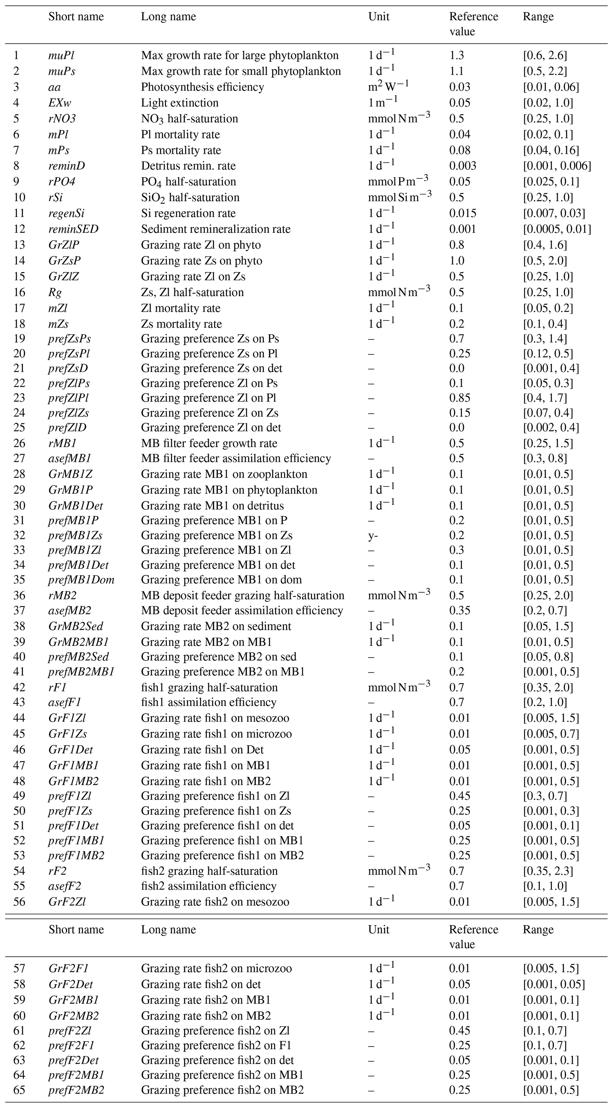
ECOSMO E2E (Daewel et al., 2019) is an extended ecosystem model of ECOSMO that includes functional group formulations for fish and macrobenthos in addition to the state variables related to nutrients, phytoplankton, zooplankton, and fish. In the original ECOSMO E2E (Daewel et al., 2019) model, the higher trophic levels included a single functional group for fish. However, the current model code includes two functional groups of fish: pelagic and demersal. In addition, the model now includes macrobenthos, which are divided into two functional groups: benthic filter feeders and benthic deposit feeders. The macrobenthos component of the model is extended to include filter feeders to account for the abundant filter-feeding macrobenthos (e.g., blue mussels, oyster beds) in the Sylt region (Asmus and Asmus, 1991; Asmus, 2011). The model parameters subjected to optimization are given in the Appendix (Table A1).

GOTM and ECOSMO E2E are configured and coupled via FABM using yaml files (gotm.yaml for GOTM and fabm.yaml for ECOSMO/ECOSMO E2E). The goodness of fit of the model is then assessed by the Willmott skill score (WSS) mean absolute error (WSS_MAE, Eq. 3) (Willmott et al., 2012).

2.3 Model configuration and setup

Study site. The Sylt Road (55.03 N, 8.46 E), located in the Sylt–Rømø Bight (SRB) to the east of the islands of Sylt and Rømø, is one of the large tidal basins of the Wadden Sea, which lies along the coastal margin of the North Sea. The SRB is drained by three tidal inlets, the Rømø Dyb, the Høyer Dyb, and the Lister Tief, all three of which meet in the Lister Ley basin, which is connected to the North Sea by a narrow opening of 2.6 km between the islands (Asmus, 2011). Two rivers, Vidå and Bredeå, flow into the bay and drain a catchment area of about 1554 km² (1081 and 473 km², respectively) (Asmus, 2011). Ecological research on fish and shellfish has been carried out in the SRB since the early 1930s, and in the 1990s extended ecosystem analyses were carried out to investigate material and energy flows in the SRB intertidal zone. While this research has contributed to our knowledge of Wadden Sea ecosystems, an overall and common view of the interlinked dynamics of material flows and the organisms has not yet been achieved (Asmus, 2011). Two-dimensional hydrodynamic and numerical models described in the 1990s remained largely limited to abiotic processes such as currents and material transport (Stanev et al., 2003; Kohlmeier and Ebenhöh, 2009). In this study, we propose a model that describes the coupled dynamics of organisms (or describes the dynamics of ecosystem processes), which will provide the necessary information and understanding to explore the hypotheses previously mentioned in the Introduction and to provide input to other models such as Ecopath-Ecosim or the ENA model (Horn et al., 2021a, b) to investigate ecosystem functioning.

GOTM. We use MERRA-2 (Modern-Era Retrospective analysis for Research and Applications, Version 2) meteorological data around the Sylt Road site. The data were downloaded from the NASA Goddard Earth Sciences (GES) Data and Information Services Center (DISC). The meteorological data include wind speed at 10 m, air pressure, air temperature at 10 m, humidity at 2 m, and shortwave radiation. The data were then processed in the GOTM format.

In this study, we did not explicitly validate the GOTM. Instead, we applied a relaxation scheme to nudge the modeled temperature and salinity towards the observations (Fig. 3), ensuring that the simulated hydrographic conditions remained consistent with the measurements. This data-assimilation-like approach was implemented to provide a dynamically constrained and physically realistic environment for the coupled ecosystem model. The observational dataset, derived from the long-term Sylt Road monitoring program, was obtained from PANGAEA (https://www.pangaea.de, last access: 15 May 2025) and served as a reference to maintain hydrographic fidelity in the simulations.

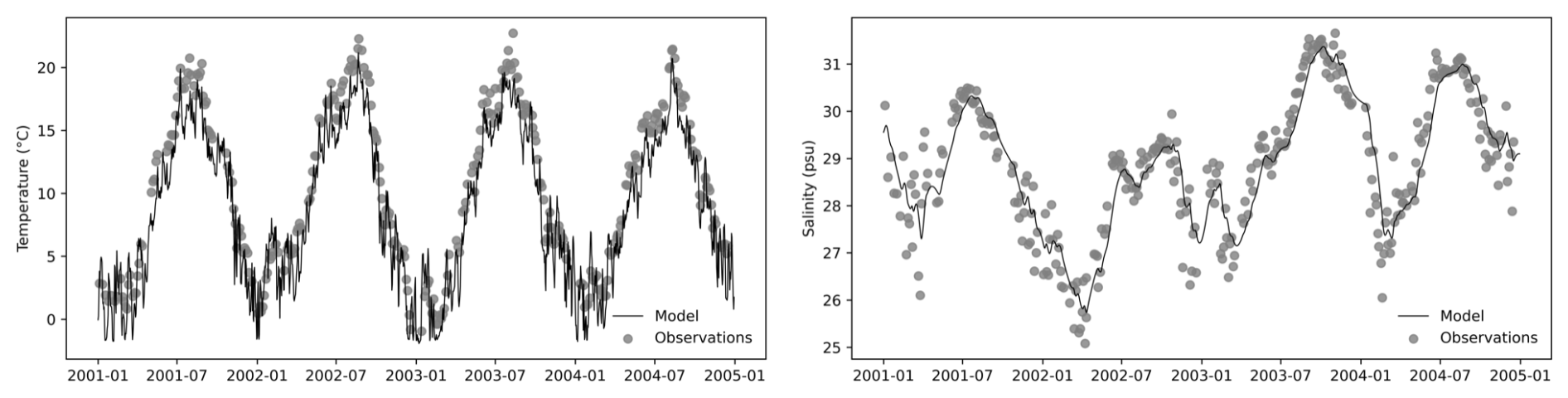
Figure 3 GOTM outputs for temperature and salinity were nudged toward observational data to ensure realistic physical conditions.

ECOSMO and ECOSMO E2E forcings and evaluation. We use data monitored at Sylt Road (55.03 N, 8.46 E) for forcing, boundary conditions, and model evaluation. Specifically, we downloaded available data from https://www.pangaea.de (last access: 15 May 2025) from 2000–2008 (8 years of data). The weekly sampling dataset includes surface temperature (^oC), salinity (psu), nutrients (nitrate (NO₃, µmol L⁻¹), phosphate (PO₄, µmol L⁻¹), silicate (SiO₄, µmol L⁻¹)), turbidity (SPM), chlorophyll a (µg Chl a L⁻¹), and zooplankton (cells per liter). Details of data sampling methods and quality control are given in Rick et al. (2023). Data were processed to the model unit (mg C m⁻³ and mg Chl a m⁻³) and written in the format required by GOTM and FABM. For zooplankton, the biomass per cell given in Martens (1975) was used to convert the number of zooplankton per liter to biomass in carbon. Processed data for study are made available in the “Data availability” section.

2.4 Model configuration and experimental parameterization setups

The ECOSMO/ECOSMO E2E model setups were configured by modifying the corresponding fabm.yaml file. We performed six experiments (detailed in Table 1) to demonstrate the PSO toolbox and to define a model that best describes the Sylt Road ecosystem. These experiments were conducted for the period 2000–2004. Probably due to the relatively short characteristic timescale of the tidally dynamic Sylt–Rømø Bight and the initial conditions derived from a stable simulation, the model reached a stable annual cycle within 1 year of simulation. Therefore, the first year was discarded as a spin-up period. The remaining 4 years (2001–2004) were used for evaluation and computation within the PSO algorithm.

Table 1 Description of the parameterization experiments. Six optimization experiments were conducted in this study to identify the model that best represents the ecosystem around Sylt Road. Parameters related to phytoplankton growth (parameters 1–4 and 6–7 as listed in Table A1) were calibrated in all six experiments. Experiments 1–3 were run with the ECOSMO model (an NPZD-type model; NPZD: nutrient–phytoplankton–zooplankton–detritus), while experiments 4–6 were run with the ECOSMO E2E model, which includes macrobenthos and fish. Experiment 1, named bt, investigated bottom-up control by calibrating parameters related to nutrients and light. Experiment 2, named tdz, investigated top-down control by calibrating parameters related to zooplankton. Experiment 3, named bttdz, investigated both bottom-up and top-down controls. Experiment 4, named bttdz_e2e_nfi, extended experiment 3 by including macrobenthos in the model. Experiment 5, named bttdzff_e2e_nfi, was similar to experiment 4, but with calibration of macrobenthos-related parameters. Finally, experiment 6, named e2e_tuned_all, included the calibration of all model parameters.

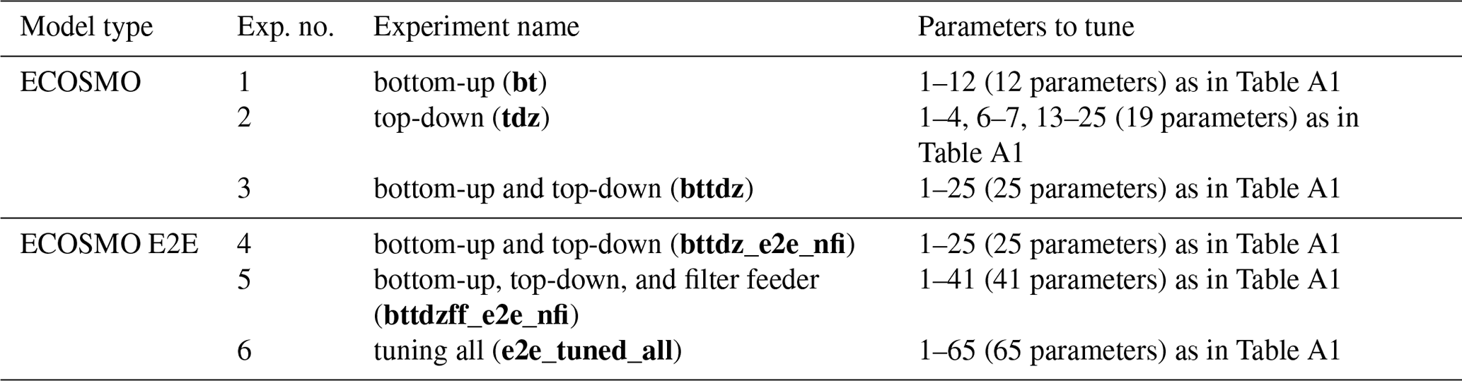
In these six experiments, we always parameterized phytoplankton-related parameters, including growth rates (muPl, muPs), mortality rates (mPl, mPs), photosynthetic efficiency (aa), and light extinction (EXw), and gradually increased the number of parameters to be parameterized and thus the model complexity. Three experiments were carried out using ECOSMO or excluding the fish and macrobenthos formulations. In the first experiment, we parameterized bottom-up processes using six parameters related to nutrients and light (half-saturation rates and water clarity). In the second experiment, we focused exclusively on top-down control processes and calibrated 13 parameters related to zooplankton (grazing rates, half-saturation rates, mortality rates, and food reference). The third experiment combined both bottom-up and top-down processes, with a total of 19 parameters. The remaining three experiments included macrobenthos and fish and transitioned to the ECOSMO E2E model. In the fourth experiment, we calibrated bottom-up and top-down processes as in the third experiment (calibration of 19 parameters) but included the macrobenthos component without calibrating it. The fifth experiment followed the fourth but included a macrobenthos calibration with 35 parameters. In the sixth experiment, we added a fish component and calibrated fish parameters, for a total of 65 parameters.

Details of the parameters tuned in each experiment, together with their corresponding ranges and reference values, are given in Tables A1. The reference values were sourced from Daewel et al. (2019), who applied a three-dimensional ecosystem to simulate the North Sea and Baltic Sea ecosystems. Since this study uses a one-dimensional model for the Sylt–Rømø Bight, where the tidal dynamics are significantly different from those in the North Sea and Baltic Sea, the reference values from Daewel et al. (2019) were not expected to produce simulation results close to optimal. To define the calibration bounds, the parameter ranges were set to half and double the reference values. The choice of parameter ranges in parameterization or optimization studies is often debated in terms of appropriateness. For studies with a limited number of parameters, literature reviews provide the most effective approach to define reasonable parameter ranges (Falls et al., 2022). However, for studies involving a larger number of parameters, ranges are typically derived from reference values (Kern et al., 2024). Given the substantial number of parameters requiring calibration in this study, we have adopted the latter approach.

For each PSO configuration, the population size per PSO iteration increased with the number of calibrated parameters. In general, the population size was at least twice the number of calibrated parameters to ensure the efficiency of the algorithm (Poli et al., 2007). Thus, the population size for each experiment was as follows: experiment 1: 30, experiment 2: 45, experiments 3 and 4: 65, experiment 5: 90, and experiment 6: 150. It should be noted that increasing the number of calibrated parameters (or the population size required per iteration) correspondingly increases the computational time of the PSO run. To avoid being trapped at a local minimum, the model parameters were perturbed four times, at the 50th, 100th, 150th, and 200th iteration.

3 Results and discussion

3.1 Demonstration of the PSO toolbox

3.1.1 Parameter identification and model skill score improvement

In optimization methods, it is generally expected that the optimizer will run until all parameters have converged. However, such runs are computationally demanding, especially when optimizing a large number of parameters (more than 10). Numerous test simulations carried out during this study have shown that reliable results can be obtained from PSO well before full parameter convergence. In Appendices A1 and A2, we show that the skill scores of the model and the evaluated state variables, as well as the converged parameter values, stabilize around the 300th iteration. Therefore, we chose the 300th iteration as the stopping condition for the PSO in the six experiments shown in Table 1.

The results of the sixth experiment (e2e_tuned_all), shown in Fig. 4a, illustrate the effectiveness of the PSO toolbox. The skill scores of the evaluated variables – chlorophyll a (Chl a), small zooplankton (Zos), large zooplankton (Zol), nitrate (NO₃), phosphate (PO₄), and silicate (SiO₄) – as well as with the overall model skill score, calculated as the sum of the evaluated variables, show significant improvement throughout the PSO iterations. In particular, the overall model improvement (shown by the black line) occurred mainly within the first 50 iterations. From the 50th to the 100th iteration, the model skill score shows a marginal increase, with the scores stabilizing after the 100th iteration. The convergence rate of the model skill score is shown in the Appendix in Fig. A6.

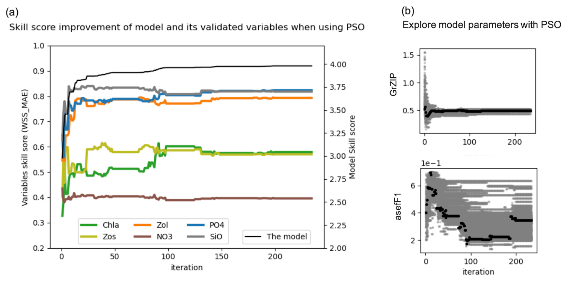
Figure 4 (a) Improvement of the skill score (WSS_MAE) of the coupled 1D GOTM–ECOSMO E2E model and its evaluated state variables over PSO iterations: the x axis represents iterations, the left y axis shows the skill scores of the evaluated state variables (Chl a, small zooplankton – Zs, large zooplankton – Zl, nitrate – NO₃, phosphate – PO₄ and silicate – SiO₄), and the right y axis shows the overall model skill score (black line), which is the sum of all evaluated state variables. (b) Exploration of model parameters through PSO iterations: the x axis represents iterations and the y axis represents parameter values. Gray dots indicate the parameter values explored, while black dots represent the best parameter values at each iteration. The figure illustrates parameter exploration for two parameters, GrZlP (grazing of large zooplankton on phytoplankton) and asefF1 (assimilation efficiency of pelagic fish), as examples. The parameter exploration may converge quickly (e.g., GrZlP) or take longer to converge (e.g., asefF1).

Parallel to the overall model improvement, the skill score improvement for the evaluated variables is mainly observed within the first 50 iterations. However, between the 80th and 100th iteration, while the overall model skill score shows a slight increase, the skill score of chlorophyll a shows a significant increase. This increase is partially offset by a decrease for other variables. In particular, among the variables evaluated, the most significant improvements are seen in PO₄, SiO, and large zooplankton, followed by Chl a and small zooplankton. Conversely, NO₃ shows minimal improvement.

In the present experiment (the sixth experiment), 65 parameters were tuned to refine the model. Examples of parameter exploration are shown for the grazing rate of large zooplankton on phytoplankton (GrZlP) and the assimilation rate of pelagic fish (asefF1) (Fig. 4b). Details of the parameter exploration for all parameters can be found in the Appendix (Fig. A3). The parameters will eventually converge if the optimization is run long enough, but reliable optimized parameters can often be obtained much earlier, before full convergence. Figure 4b illustrates that the parameters can converge quickly (e.g., in the case of GrZlP) or take much longer to converge (e.g., in the case of asefF1). The speed of convergence is likely to depend on the availability of relevant data used in the cost function. However, we cannot draw definitive conclusions about the speed of convergence. Our parameter exploration (Fig. A3) showed that some parameters relevant to the available data converged rapidly (e.g., muPl (maximum growth rate of large phytoplankton), GrZlP (grazing rate of mesozooplankton on phytoplankton), and GrZsP (grazing rate of microzooplankton on phytoplankton)), while others relevant to the same data converged slowly (e.g., mPl (mortality rate of large phytoplankton), rPO4 (half-saturation rate of phosphate), and rSi (half-saturation rate of silicate)). In addition, parameters for which there were no relevant data for evaluation also showed a rapid convergence (e.g., GrF1MB2 (grazing rate of pelagic fish on deposit feeder), rMB1 (half-saturation rate of filter feeder), and rMB2 (half-saturation rate of deposit feeder)). Apart from the data available to constrain the parameters, the convergence speed of the optimization algorithms can be influenced by the sensitivity of the model parameters. Parameters that have a significant effect on the model output will typically require more iterations to converge, as the optimization process has to account for their large effect. Conversely, parameters with minimal influence may lead to faster convergence due to their limited effect on the model behavior. A study by Fennel et al. (2001) found that models with parameters of high sensitivity require more calibration effort to achieve accurate predictions. Razavi and Gupta (2016) discussed the importance of sensitivity analysis in environmental modeling, highlighting that parameters with high sensitivity can dominate model behavior and therefore require careful consideration during model calibration. Therefore, further research is likely to be required to clarify the relationship between velocity parameter convergence, data availability, and model parameter sensitivity.

Compared to other optimization algorithms, such as the biased random key genetic algorithm (BRKGA) studied by Falls et al. (2022), which reached convergence within the first 10–20 iterations, the PSO algorithm showed a slower rate of convergence. This difference can be attributed to several factors. First, the basic nature of the algorithms is different. PSO is a population-based optimization technique in which particles explore the search space and iteratively adjust their positions based on both their own experience and that of their neighbors. As a result, PSO often requires a greater number of iterations as the particles incrementally refine their positions towards the optimal solution while balancing exploration and exploitation. In contrast, BRKGA showed faster convergence due to its ability to efficiently guide the search towards promising regions early in the optimization process. However, this advantage comes at the cost of a higher probability of getting trapped in local minima. In addition, the biased selection mechanism in BRKGA facilitates rapid population improvement, which further accelerates convergence. Second, the initialization strategies of the two algorithms were different. The BRKGA may start with near-optimal solutions, thus requiring fewer generations to reach convergence. In contrast, PSO initialized with a wider range of parameter estimates, requiring additional iterations for refinement. Third, PSO was calibrated with a larger number of parameters compared to BRKGA – 65 and 9, respectively. The higher dimensionality of the PSO increases the complexity of parameter calibration, potentially prolonging convergence. In contrast, the lower number of parameters in BRKGA results in a more constrained search space, further contributing to its faster convergence.

In order to fully assess the performance of particle swarm optimization (PSO) in comparison to other optimization techniques, an ideal approach would be a quantitative comparison with the other techniques, such as genetic algorithms (GA), simulated annealing (SA), and Bayesian optimization (BO), within the same case study of the Sylt–Rømø Bight. However, such a comprehensive comparison is beyond the scope of this study. Instead, based on a qualitative assessment of the strengths and limitations of each method, the PSO was selected primarily because of our previous experience with the algorithm and its demonstrated ability to efficiently handle high-dimensional parameter spaces (up to 65 parameters in this study) while ensuring rapid convergence. The PSO is particularly well suited to this optimization problem because it effectively balances exploration and exploitation through velocity updates, offering greater computational efficiency than GA, which requires a large number of function evaluations due to crossover and mutation operations. While SA is advantageous for escaping local minima, its inherently slow convergence makes it impractical for high-dimensional problems. To further enhance the robustness of the PSO, we incorporate a periodic perturbation mechanism that resets the particle velocities after a predefined number of iterations. This adjustment exploits the strength of SA in escaping local minima, while preserving the fast convergence advantage of PSO. Although BO is highly efficient in low-dimensional spaces, its computational cost increases significantly with increasing dimensionality due to the complexity of updating surrogate models. Given these considerations, PSO emerges as a particularly effective choice for optimizing complex biogeochemical model parameters in this study.

3.1.2 Potential model parameter ranges

As shown in Fig. 4a, the model skill score stabilizes after the 100th iteration, although small fluctuations in the skill score of the evaluated variables persist over the next 50 iterations. This suggests that the parameter set from the 100th iteration provides a similar goodness of fit for the model. We have extracted the best parameter values from this iteration (black dots), as shown for GrZlP and asefF1 in Fig. 4b, and plotted these values in Fig. 5. It can be seen that about two-thirds of the tuned parameters each converge to their respective values. The parameters with the largest ranges are predominantly associated with fish or macrobenthic elements, which represent the highest trophic levels and ultimately the closure terms within the model. The use of closure terms to address model–data mismatch is a common practice in modeling. In addition, the lack of data to constrain the macrobenthic and fish parameters allows these parameters to vary freely during parameterization, resulting in greater uncertainty. Overall, Fig. 5 shows that the PSO toolbox can define specific values for some parameters and suggest possible ranges for others.

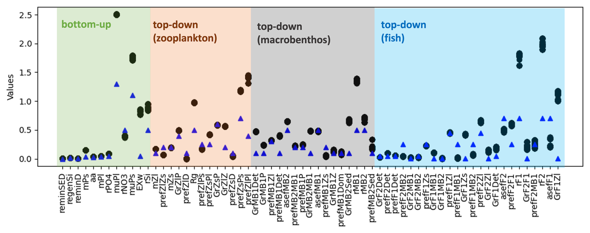
Figure 5 Potential parameter values and their corresponding ranges, as suggested by the PSO toolbox, are shown. The black dots represent the optimal parameter values obtained from the 100th iteration onwards, up to the final iteration, as shown in Fig. 4b for GrZlP and asefF1. The blue triangle points are the reference parameter values of the model.

Several model parameters were calibrated to their upper bounds to optimize the model performance, including the growth rates of large (muPl) and small (muPs) phytoplankton, the half-saturation constants for pelagic (rF1) and demersal fish (rF2), the half-saturation constant for filter feeders (rMB1), and the grazing preferences of microzooplankton for small phytoplankton (prefZsPs) and mesozooplankton for large phytoplankton (prefZlPl). The elevated values of muPl and muPs can be attributed to limitations inherent in both the 1D model and the input data. Phytoplankton growth in the model follows Liebig's law of the minimum (Schrum et al., 2006), where the most limiting factor restricts growth. As the MERRA-2 reanalysis data underestimates shortwave radiation (Yingshan et al., 2022), which is used to force the model, it is likely to result in lower simulated light levels compared to reality, thereby suppressing phytoplankton growth. To compensate for this reduced growth potential and reproduce the observed phytoplankton biomass, muPl and muPs were parameterized to higher values. The high values of rF1, rF2, rMB1, prefZsPs, and prefZlPl are likely a consequence of their representation at higher trophic levels, with closure terms applied to these parameters to account for model–data discrepancies. Given the inherent limitations of any model, including the inability to represent all real-world processes and the lack of sufficient data to fully constrain parameter values, it is crucial to interpret these parameters in light of model simplifications and data availability.

3.1.3 PSO optimized parameter set for the ecosystem around Sylt Road

As the model skill score stabilized from the 100th iteration, we selected the parameter values from the 100th iteration as the optimal parameter set for the coupled 1D GOTM–ECOSMO E2E model to simulate the ecosystem around Sylt Road. We ran two models: one with the parameter set from the 100th iteration (named model_pso) and one with the default parameters (shown as blue triangle points in Fig. 5) before applying PSO (named model_ref) for the period from 2000–2008. The year 2000 was excluded as a spin-up period. The period from 2001–2004 (shown in the shaded part of Fig. 6) was used in the PSO experiments (1). Consistent with the improvement in skill scores, the model_pso output for PO₄ and large zooplankton (mesozoo) (represented by the black line) over the period 2001–2004 closely matches the observational data (represented as gray dots). In addition, the model with the optimal parameter set from PSO captures the seasonal cycle of SiO better, although to a slightly lesser extent. The model effectively simulates the spring phytoplankton bloom, which is a distinct and significant event characterized by a substantial increase in biomass. However, it struggles to reproduce the lower-magnitude blooms that occur at other times of the year, such as in summer or autumn. In parameterization, the primary objective is often to capture the key feature of the system dynamics. Accordingly, model parameters were initially calibrated with a focus on these high-biomass events. As a result, the calibration may have reduced the ability of the model to represent or capture blooms at other times of the year. In contrast to phytoplankton, the model performs well in simulating the dynamics of small zooplankton (microzooplankton) and shows good agreement with observed data. Comparing the performance of the default model (represented by the blue line) with that of the model after parameter optimization via PSO, there is a clear improvement in the latter, which shows significantly better agreement with observed data.

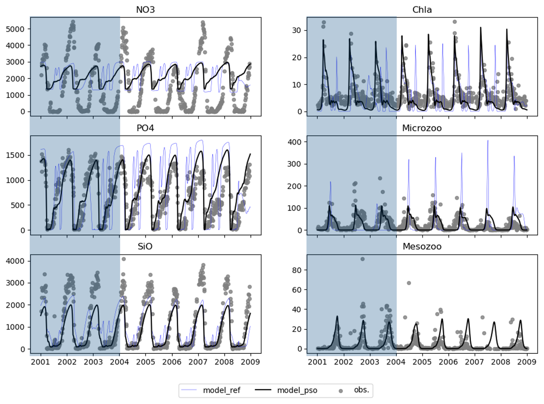
Figure 6 Model outputs (black line) using the parameter set found by PSO at iteration 100 and observations (solid gray dots) from 2001–2008, where 2001–2004 was the tuning period and 2005–2008 showed how well the parameter set worked in other periods.

As indicated by the NO₃ skill score, the model faces challenges in resolving NO₃ to match observations. While the model reproduces the seasonal cycle of NO₃, it fails to capture both the magnitude and the period of NO₃ removal. There are several reasons for this discrepancy. Firstly, the model setup does not account for nutrient loads from rivers entering the Sylt–Rømø Bight. Secondly, the one-dimensional (1D) model does not take into account horizontal advection, which prevents the transport of nutrients and other materials to and from the site. Thirdly, the ECOSMO model, and thus the ECOSMO E2E model, simplifies the representation of the sediment processes. As already discussed in Daewel and Schrum (2013), this could lead to reduced phosphorus release from sediments under oxic conditions. As a consequence, the system becomes phosphorus-limited, inhibiting further nitrogen removal during blooms. Therefore, the discrepancy in nitrate is likely due to the limitations of the 1D model setup and cannot be resolved by parameterization alone.

Analysis of the model output for the period 2005–2008 (the unshaded part of Fig. 6) shows that the optimal parameters identified for the period 2001–2004 continue to perform well over a longer period. This suggests that the parameter set is robust or that the simulated period (2005–2008) has a similar cycle to the previously parameterized period (2001–2004).

The optimized model seems to capture the mean seasonal cycle better but still fails to reproduce the interannual variability. This limitation may be due to the lack of high-resolution data for model evaluation. Figure 6 may give the impression that high-resolution observations are available for validation, but closer inspection reveals significant gaps in the data, with many days within a year missing observations. Even after merging 4 years of data into a single composite year, daily coverage was not achieved. It is likely that this data limitation has influenced the model optimization process, making it more biased towards the mean state while failing to represent interannual variability. Addressing this issue may require alternative approaches, such as data assimilation techniques or the inclusion of additional observational datasets to better constrain interannual variability.

3.2 Multiple parameter sets can reproduce observations equally well despite differences in values

As shown in the previous section, a large number of parameter sets reproduce the observational data equally well. To explore these parameter sets in more detail, we focus on model runs using parameters extracted from iterations 100–300 at intervals of 5 (see Fig. 6). Despite notable differences in parameter values, such as asefF1, GrF1Zl, GrF2F1, and rSi, the skill score and evaluated state variables of the model remain relatively unchanged (see Fig. 4). The outputs generated by these parameter sets show almost identical characteristics, with minor variations observed for ammonia (NH₄) and flagellate biomass (in chlorophyll a). Notably, significant parameter differences occur mainly in fish-related parameters (specifically asefF1, GrF1Zl, and GrF2F1). The slight increase in rSi, the half-saturation rate of silicate, is not sufficient to significantly affect phytoplankton biomass. Fish biomass is close to zero in all model outputs (not shown) due to the PSO setting its half-saturation rate high, resulting in minimal growth. While acknowledging the inaccuracies of this approach, the lack of data to inform fish-related parameters, compounded by the complexity of the closure terms as discussed above, contributes to the unresolved discrepancies between the model and observational data.

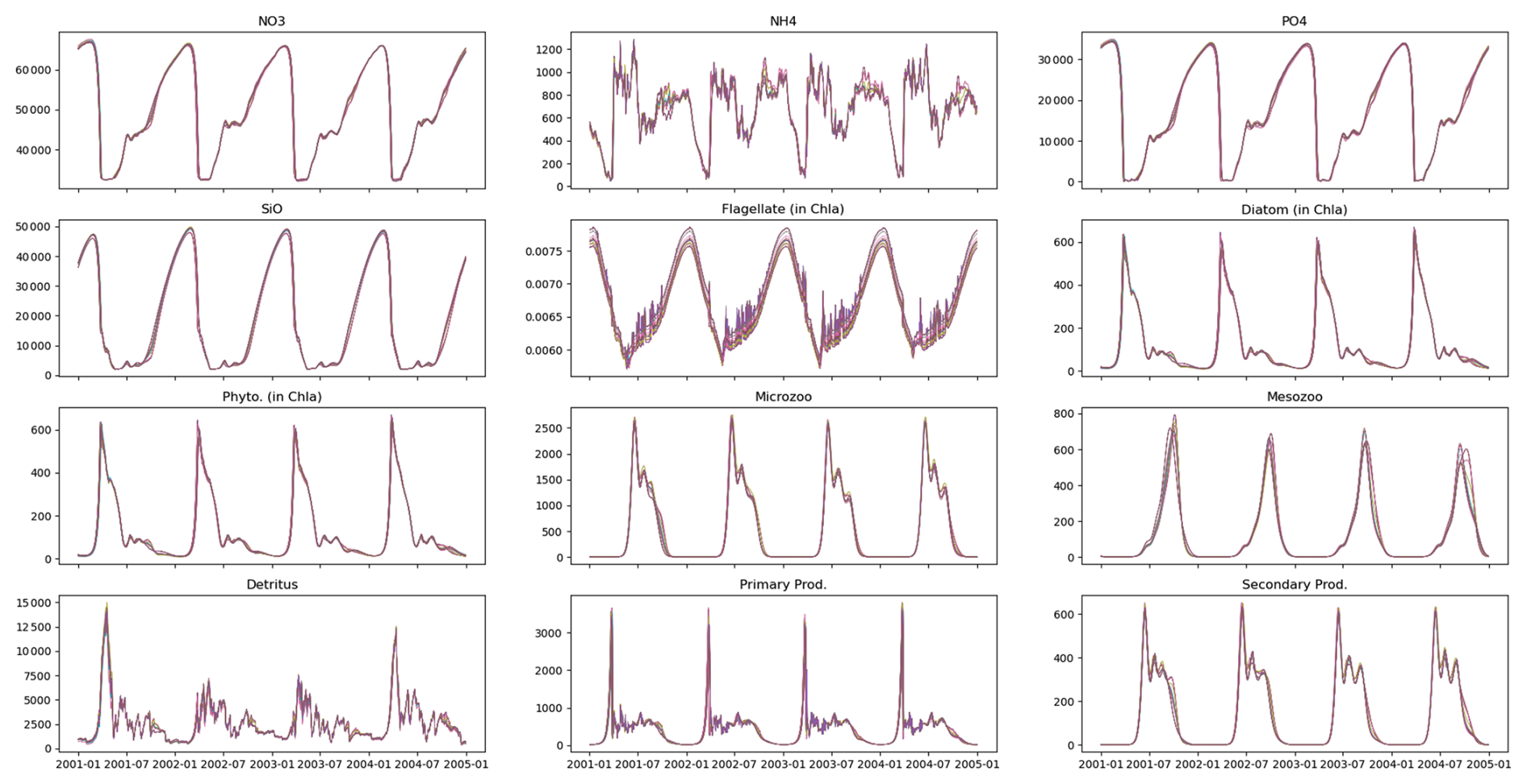
Figure 7 Multiple parameter sets can reproduce observations equally well despite differences in their values. The lines represent the output of 40 model runs, each using a different parameter set, evaluated between the 100th and 300th iteration at intervals of 5. Although these parameter sets differ in their values (Fig. A3), they produce similar results.

In this study, no differences were observed between the model runs despite variations in their parameter sets (Fig. 7). In a similar study using particle swarm optimization (PSO) to parameterize a 1D biogeochemical model of Puget Sound (Nguyen, 2021), marked differences were reported in model output between parameter sets that achieved equally good fits to observations. The results of the Puget Sound study were reprinted here in an Appendix to highlight examples where PSO can elucidate different systems capable of reproducing identical observations. The Puget Sound study examined two parameter sets that differed in phytoplankton growth (growth rate, I₀, mortality), zooplankton (mortality), and detritus (sinking) (see Fig. A4), resulting in notable disparities in carbon transfer between trophic levels (via grazing) and carbon export (via sinking) (see Fig. A5). These disparities imply that systems with completely different dynamics can yield equivalent goodness of fit to observations.

This issue of multiple parameter sets reproducing observations equally well, despite differences in values, is a fundamental challenge in parameterization and is often referred to as equifinality (Beven and Freer, 2001). The critical question is whether similar model outputs arise due to mutually compensating processes or low parameter sensitivity. On the one hand, many studies have identified low sensitivity, where model outputs show minimal variation in response to changes in certain parameters, as a key factor contributing to this phenomenon (Gábor et al., 2017; Pant, 2018; Mai et al., 2020). The work on sloppiness in model simulations suggests that some parameters have little influence on model behavior, allowing a wide range of values to produce comparable results (Monsalve-Bravo et al., 2022). On the other hand, some studies (particularly in fields such as manufacturing and robotics; Marini and Corney, 2021; Chen et al., 2017) have found mutually compensating processes, where variations in some parameters are offset by adjustments in others, leading to similar model outputs despite different parameter combinations. Understanding the underlying cause of equifinality, whether low sensitivity or process compensation, is critical to developing robust optimization strategies and ensuring accurate model predictions. To address this challenge, sensitivity analyses (e.g., Saltelli et al., 2008; Gábor et al., 2017) are essential to distinguish between process compensation and insensitivity-driven equifinality and to ensure that parameter estimation efforts are focused on the most influential variables. We therefore plan to conduct local and/or global sensitivity analyses as suggested by Saltelli et al. (2008) and Gábor et al. (2017) to identify highly constrained parameters. This approach will refine parameter selection and enhance the robustness of our optimization strategy, ultimately improving model reliability and predictive performance.

The identification of different parameter sets may result from limitations in the model or optimization method, but it also provides an opportunity to explore alternative system states that are not yet fully understood. Our ability to observe these states is limited by current knowledge and measurement techniques, but this does not mean that our understanding is absolute or unchanging. The presence of multiple parameter sets may indicate alternative system configurations that have not yet been considered or observed. It also suggests that significant perturbations to the system could cause it to shift to an entirely different state. While it is crucial to ensure that the model does not produce correct results for the wrong reasons, the ability to identify multiple parameter sets remains valuable. It provides important insights into system dynamics, provided the results are interpreted carefully in the context of model limitations and uncertainties.

3.3 Optimizing model complexity with PSO: top-down control by macrobenthos in the marine ecosystem around Sylt Road

Figure 8 shows the model outputs obtained from runs using the best parameter sets identified by the PSO across six experiments detailed in Table 1. The black line represents the sixth experiment, previously shown in Fig. 6, which shows a good fit to the observations. The first experiment (bottom-up control, bt) highlights the limitations of relying solely on bottom-up processes. Despite PSO parameter optimization, the model fails to match the observations, suggesting that adjustments to bottom-up processes alone are insufficient to achieve model accuracy. The second experiment (tdz), which tunes top-down (zooplankton) control parameters, leads to partial improvements, but the model still does not fully match the observed dynamics. The third experiment (bttdz), which incorporates both bottom-up and top-down parameters, leads to marginal improvements, highlighting the dominance of top-down processes in improving model fitness.

Figure 8 Model results of six PSO experiments described in Table 1. The black line represents the sixth experiment, which tuned all parameters (e2e_tuned_all), as previously shown in Fig. 6. The model outputs of the parameters from the sixth experiment showed a good fit to the observations.

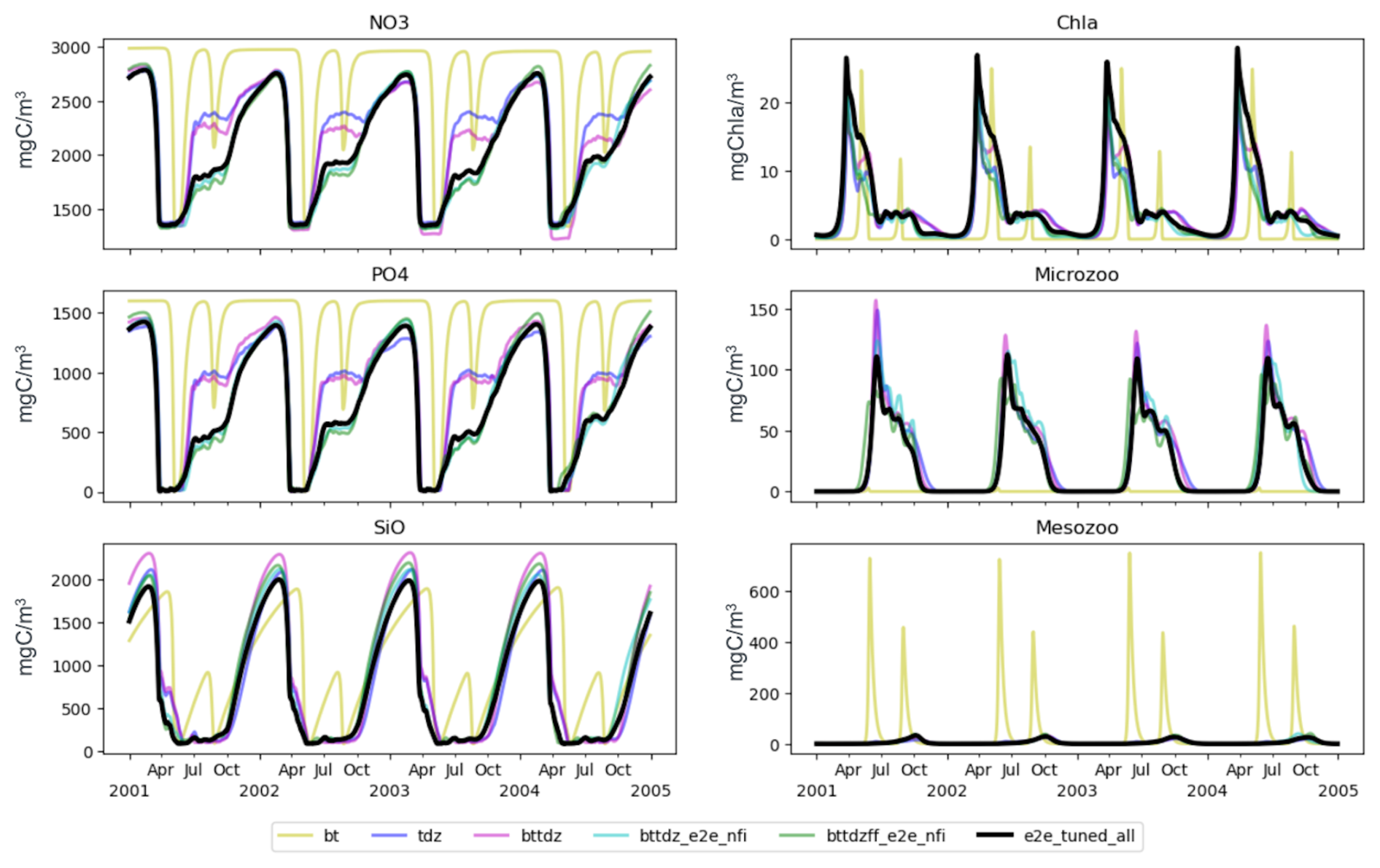
A crucial turning point appears in the fourth experiment (bttdz_e2e_nfi), which includes macrobenthos (filter feeders and sediment feeders) without tuning. This experiment produces results that closely resemble those of the sixth experiment, indicating the crucial role of macrobenthos in accurately reproducing observations. This finding is consistent with observations from the Sylt–Rømø Bight ecosystem, where mussel beds exert a substantial influence on phytoplankton and trophic interactions (Asmus and Asmus, 1991; Baird et al., 2007). The fifth and sixth experiments, which include additional macrobenthos tuning and fish, show marginal gains over the fourth experiment, reinforcing the notion that increased model complexity does not necessarily result in better model performance.

This study highlights the use of PSO to optimize model complexity. By using PSO, we are able to systematically test and identify the optimal level of model complexity – avoiding overfitting while maintaining ecological relevance. This unified framework for model optimization allows us to balance the exploration of different model complexities with the exploitation of the most influential parameters, ultimately resulting in the most accurate model representation. The PSO methodology provides a computationally efficient way to test and refine model complexity, ensuring that we do not introduce unnecessary parameters that do not improve predictive accuracy.

By evaluating the model fit at different levels of complexity, we show that the inclusion of macrobenthos is a key factor in improving model performance, while the inclusion of fish dynamics provides limited additional benefit. This optimization-driven approach provides insight into the ecological structure of the Sylt–Rømø Bight ecosystem given the available observations, highlighting the importance of targeted complexity in ecosystem models. Previous studies (Huse and Fiksen, 2010; Fulton et al., 2003; Friedrichs et al., 2007; Fulton, 2010) have also suggested that adding complexity to a model is not always beneficial or necessary. Our findings support the notion, articulated by Kuhn and Fennel (2019), that identifying the appropriate level of complexity is essential for developing models that faithfully represent biogeochemical cycles across both spatial and temporal scales. Importantly, this study illustrates how PSO allows us to fine-tune the complexity of the model, ensuring that we include only the most ecologically relevant processes for accurate predictions.

4 Conclusions

The particle swarm optimization (PSO) toolbox has demonstrated its effectiveness in identifying parameter values that generally reproduce the Sylt observations, with the exception of the nitrate magnitude. This discrepancy is probably due to the limitations of the 1D model in resolving the hydrodynamic complexity in the Sylt–Rømø Bight (e.g., tidal flats) and the lack of river inputs in the model setup. The toolbox, written in Fortran90, has proven to communicate effectively with models or coupled models within FABM by simply invoking the model executable (created after compilation) in FABM.

While some adjustments to the toolbox code, such as the cost functions (or model skill score) and other factors, may be required due to variations in model outputs and simulation periods, the underlying algorithm remains adaptable. Detailed instructions on what changes to make and where to make changes to the toolbox to adapt it to new model simulations are can be found in the toolbox repository at https://codebase.helmholtz.cloud/hoa.nguyen/parameterisation (last access: 16 May 2025).

In addition to parameter identification, we have shown that the parameterization is able to find alternative Sylt ecosystems that fit the observational data equally well, providing different perspectives on the ecosystem under study. Furthermore, the toolbox is able to define an optimal model for the ecosystem around the Sylt Road.

Despite its robustness, the effectiveness of the toolbox depends on the availability of data to identify model parameters and the computational resources required to run the algorithm. The toolbox is currently suitable for fast-running models, with execution times ranging from seconds to several minutes. However, it is not well suited to large models with higher computational requirements, such as those that take hours to run. For these models, advanced methods may be required, highlighting the continuing need for advances in optimization techniques.

In summary, the toolbox has the following advantages.

1. Improved goodness of fit of marine ecosystem models: the application of the particle swarm optimizer (PSO) to biogeochemical modeling leads to significant improvements in model accuracy and overcomes the challenges associated with traditional parameterization techniques (trial and error).

2. Reusability and accessibility: the implementation of a PSO compatible with the Framework for Aquatic Biogeochemical Models (FABM) opens up opportunities for further optimization applications to models in the FABM. This will encourage the practice of model parameterization to improve model accuracy.

3. Insights into model complexity and versatility: the study of model complexity suggests the optimal representation of an ecosystem. The identification of different parameter sets with equally good fits to observations demonstrates the robustness and versatility of the toolbox.

It also has the following limitations.

1. The parameter set is only valid for the system under consideration. It may be applicable to nearby systems with similar environmental and hydrodynamic conditions. However, for systems with different conditions, re-parameterization is necessary. A colleague of ours attempted to apply the Sylt parameter set to an ecosystem in the central North Sea but failed to reproduce the ecosystem accurately. This failure is attributed to the differences in the light climate and nutrients between the central and shallow coastal North Sea.

2. Data constraints and model limitations: a major challenge in ecosystem modeling is the availability and quality of data required to inform and constrain the model. This limitation is not unique to the method presented but is a common obstacle in all modeling efforts. The accuracy of the parameterization toolbox is inevitably linked to the completeness and reliability of the data available.

3. The challenge of computational efficiency arises with the number of tuned parameters. While the particle swarm optimization (PSO) toolbox demonstrates efficiency in parameterizing models, it is important to recognize its limitations in terms of computational time. The runtime of the toolbox depends on the number of parameters to be tuned, as more model evaluations are required. For example, the first experiment (12 parameters) took 17 h to run, while the sixth experiment (65 parameters) took 5 d. Although it is suitable for models with a moderate number of parameters, its applicability decreases when dealing with an extensive parameter set. This limitation requires a pragmatic consideration of model complexity and a judicious selection of parameters for optimization to ensure computational feasibility.

4. Speed dependence on model runtime: a notable limitation of the PSO toolbox is its sensitivity to model runtime. While the method performs exceptionally well with fast-running models (i.e., seconds to a few minutes), it faces significant challenges with slower-running models (i.e., hours or days). Although the theoretical feasibility of the method remains intact, its practicality is significantly reduced due to longer execution times. This issue highlights the need for methodological adaptations or alternative approaches when dealing with models characterized by extended runtime.

5. This study examines the relationship between observations, constrained and unconstrained parameters, the number of parameters selected for optimization, and model complexity. In Sect. 3.1, we were unable to explain why some parameters converged earlier than others based on the availability of observations. We suggest further investigation of the relationship between observation availability and parameter sensitivity, as well as the effects of parameter selection and model complexity on optimization. This would provide a comprehensive guide to model optimization.

For future work, we plan to undertake the following tasks to apply the toolbox and address the current limitations of the toolbox.

1. Apply the PSO parameterized 1D GOTM–ECOSMO E2E for the Sylt–Rømø Bight in the case shown above to test the hypotheses that (i) warmer winters lead to shifts from a pelagic to a more benthic-dominated food web, (ii) there is enhanced top-down control during warm winters by predators (e.g., blue mussels, oysters, razor clams), and (iii) bare mussel beds and mussel cultures reduce the standing stock of phytoplankton but also promote phytoplankton primary production.

2. Although we have successfully demonstrated the capability of the PSO in parameterizing the Sylt–Rømø Bight ecosystem model, the model was tuned towards a mean state, resulting in an underrepresentation of interannual variability. This is mainly due to the low resolution of the data. In addition, the limited period of data availability (8 years) in this case study prevents the PSO from demonstrating robustness over longer decadal or multi-decadal timescales. We intend to apply the PSO in other studies with rich and high-resolution data, such as the study conducted by Yumruktepe et al. (2023), to improve the robustness of the PSO over longer simulation periods.

3. Further investigation of the relationship between observational constraints and parameter values, as well as the number of parameters selected for optimization and model complexity, is needed to provide comprehensive guidance on model optimization.

4. Application of optimization to 3D biogeochemical models: as mentioned above, the current toolbox is suitable for 1D (or fast-running) models but is not yet practical for 3D models. Although the toolbox theoretically works for 3D models, the runtime is currently impractical. We plan to improve our existing toolbox to increase its speed and are also open to incorporating new methods suitable for 3D optimization into the toolbox.

Appendix A

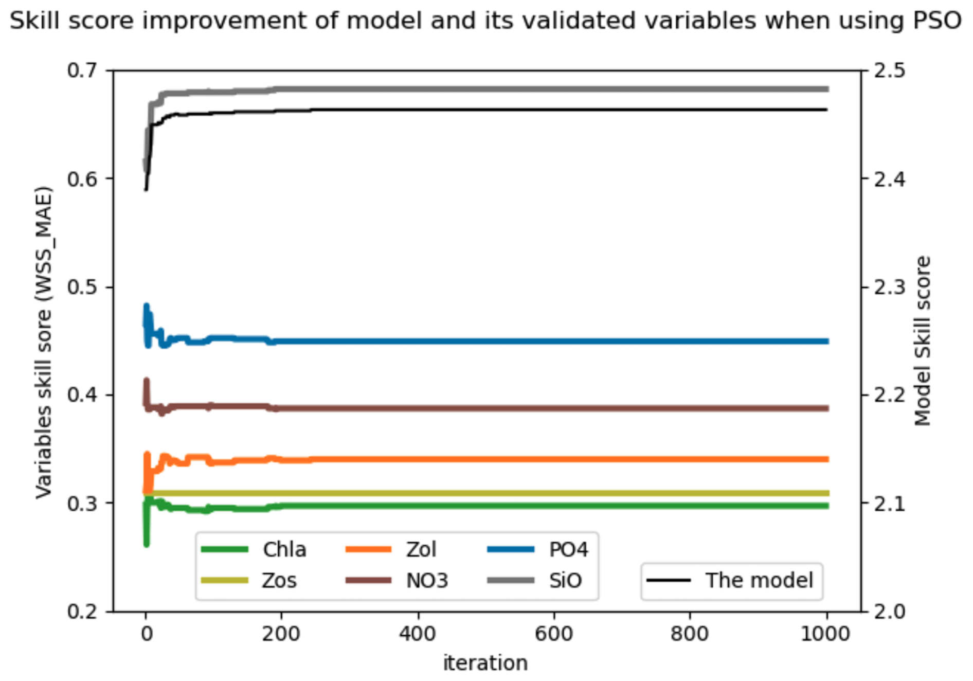
Figure A1 Model and its variable skill scores of the first experiment with PSO. The experiment illustrated that the skill scores highly improve in the first 50 iterations; after that they are only slightly improved, and around the 200th iteration, the skill scores are stabilized even though parameters still fluctuated much longer.

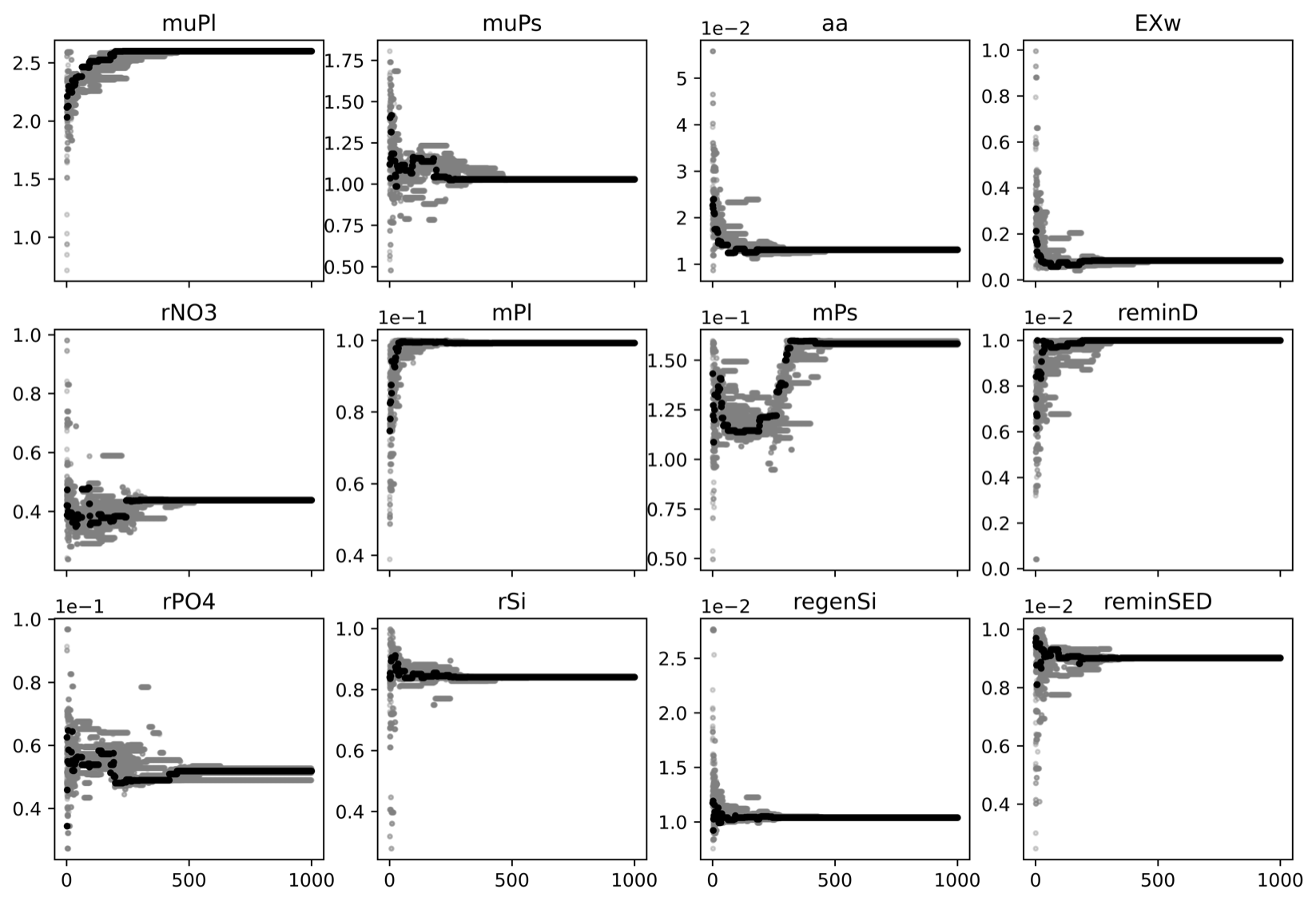
Figure A2 PSO parameter exploration of the first experiment. The x axis is the iteration, and the y axis is the parameter value. In a given iteration, gray dots are parameter values tried and the black dot represents the parameter values that give a model best fit to the observation at the iteration. This experiment illustrated that a reliable optimized parameter set (as an output of the PSO) can be achieved much earlier (i.e., around the 300th iteration) than at the converged point (e.g., the 1000th iteration).

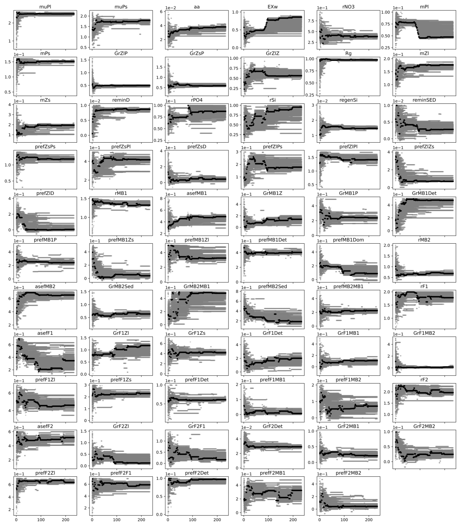
Figure A3 PSO parameter exploration of the sixth experiment. The x axis is the iteration, and the y axis is the parameter value. In a given iteration, gray dots are parameter values tried and the black dot represents the parameter values that give a model best fit to the observation at the iteration.

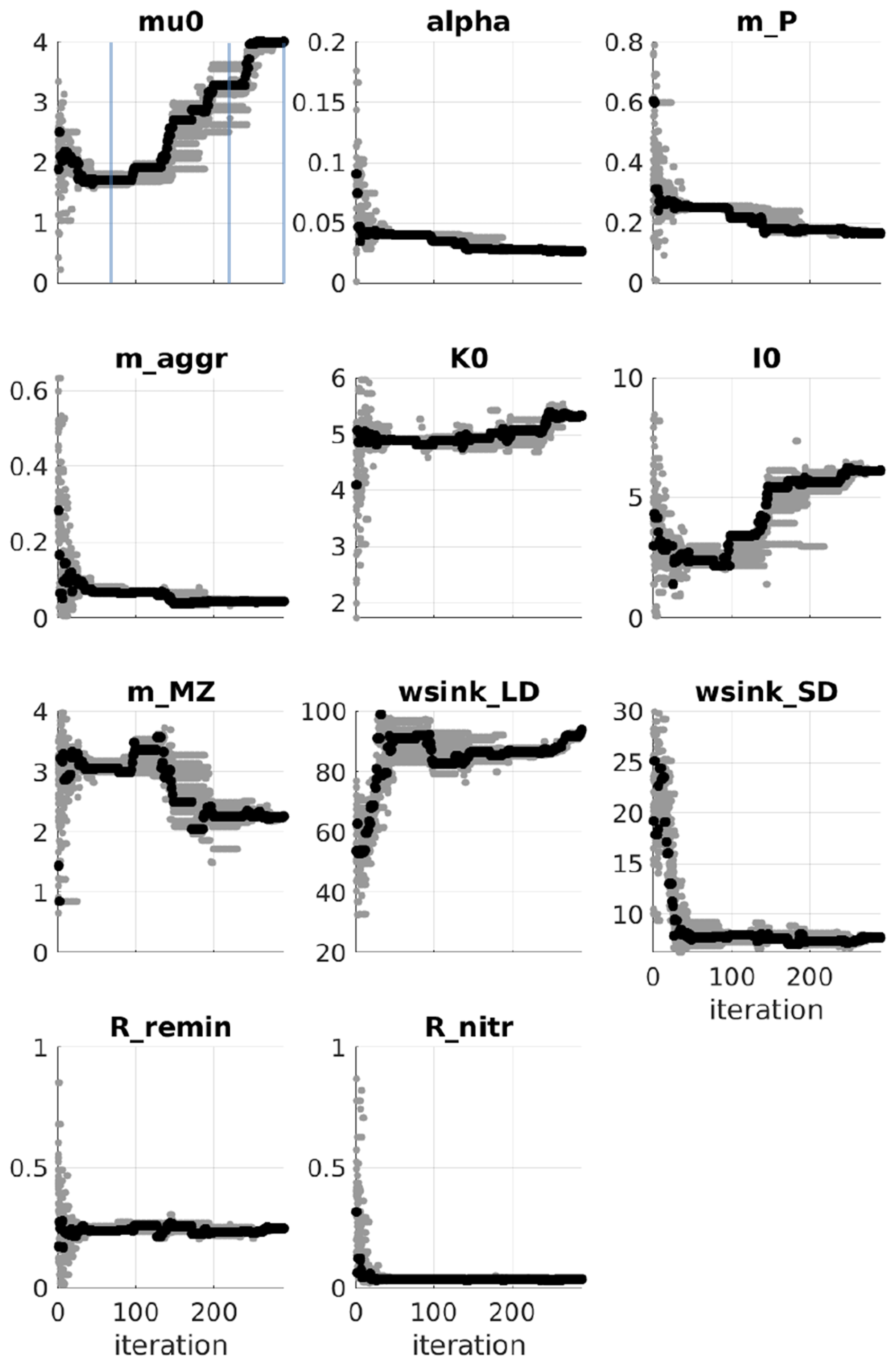
Figure A4 PSO for the Puget Sound ecosystem model (Nguyen, 2021). Parameter exploration: in a given iteration, gray dots are parameter values tried and the black dot represents the parameter values that give a model best fit to the observation at the iteration. Blue lines mark the iteration number: 70, 220, and 300. (The figure is used with permission.)

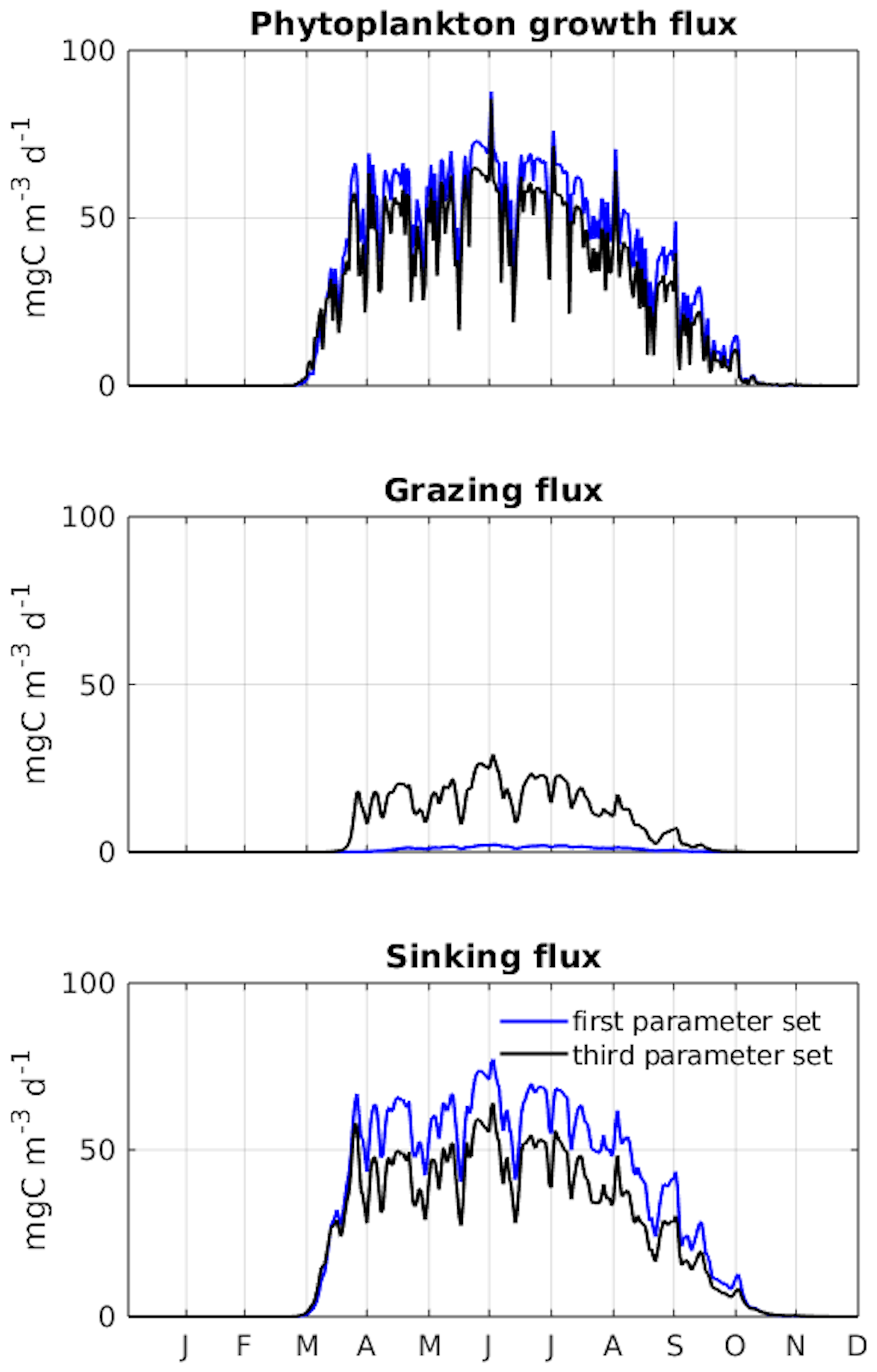
Figure A5 PSO for the Puget Sound ecosystem model (Nguyen, 2021). Differences in dynamics between the two parameter sets which produce similar model goodness of fit are shown. The first and third parameter sets are taken at the 70th and 220th iteration as marked in Fig. A4. The figure shows a clear difference in carbon transfer between trophic levels (via grazing) and carbon export (via sinking) between the two parameter sets. (The figure is used with permission.)

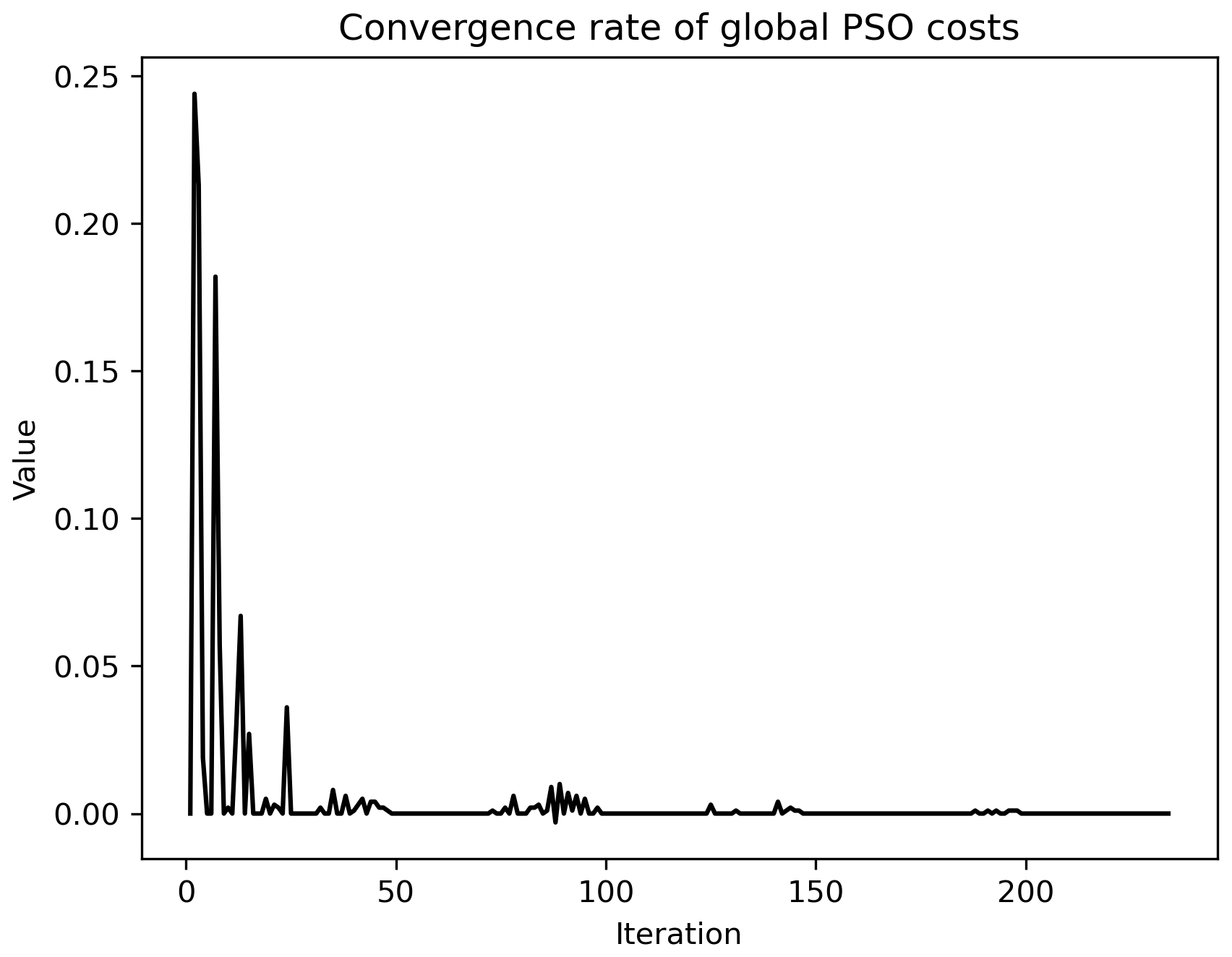
Figure A6 Rate of convergence of the model (black line, unit: 1 d⁻¹) given in Fig. 4a. After the 100th iteration, the convergence rate approached zero.

Table A1 ECOSMO and ECOSMO E2E model parameters.