Top-down CO emission estimates using TROPOMI CO data in the TM5-4DVAR (r1258) inverse modeling suit

Carbon monoxide in the atmosphere adversely affects air quality and climate, making knowledge about its sources crucial. However, current global bottom-up emission estimates retain significant uncertainties. In this study, we attempt to reduce these uncertainties by optimizing emission estimates for the second half of the year 2018 on a global scale with a focus on the Northern Hemisphere through the top-down approach of inverse modeling. Specifically, we introduce observations from the TROPOspheric Monitoring Instrument (TROPOMI) into the TM5-4DVAR model. The emissions are further constrained using NOAA surface flask measurements. We conducted six experiments to investigate the impact of data use in our inversions, varying the a priori emissions and observational datasets.

Notably, the inversion driven by satellite observations alone agrees with flask measurements south of 55° N almost as well as the inversions that included those measurements. This indicates that our method could be suitable for inversions based purely on satellite observations. Compared to the bottom-up estimates, all experiments result in strong (up to 75 %) broad-scale emission reductions in China and India throughout the entire inversion period. Part of the reduction in China can be attributed to policy and technology changes (e.g., coal to gas). Additionally, the OH climatology used to simulate chemical loss appears to be underestimated in that region, which also skews the inversions towards lower emissions. In the experiments that include the surface flask measurements, we find strong localized emission increments over Europe and the Sahara, which are traced back to limitations of the model in reproducing point measurements on mountain tops.

1 Introduction

Carbon monoxide (CO) is toxic (Ryter et al., 2018) at high mixing ratios (>9 ppm for an exposure of 8 h; much shorter at even higher mixing ratios, according to the World Health Organization; WHO, 1999). However, CO mixing ratios in the atmosphere are usually low enough that its toxicity and the resulting direct health effects are overshadowed by its indirect effect on air quality. Most notably, CO is an ozone (O₃) precursor in the presence of nitrogen oxides (NO_x) and solar radiation (Holloway et al., 2000). The resulting tropospheric O₃ is also detrimental for the health of humans and plants alike, even at low mixing ratios (>120 ppb for an exposure of 1 h; or less for a longer exposure; Mckee, 1993). Most CO will eventually be converted to carbon dioxide (CO₂) via reaction with the hydroxyl radical (OH) (Logan et al., 1981). As such, CO reduces the oxidative capacity of the atmosphere and both directly (by formation of CO₂) and indirectly (through the reduced OH abundance and thus longer methane, CH₄, lifetime) increases greenhouse gas loads (Raub and McMullen, 1991; Daniel and Solomon, 1998; Heilman et al., 2014). As for the sources of atmospheric CO, almost half of it comes from the oxidation of methane and (non-methane) volatile organic compounds (NM)VOCs, i.e., secondary CO production. The rest comes mostly from incomplete combustion of fossil fuels and biomass (e.g., wildfires or domestic wood burning) but also, in smaller quantities, from direct emissions from plants (biogenic CO) and the oceans (Zheng et al., 2019). While biomass burning makes up less than a quarter of the total CO source in most years, those emissions come with the largest uncertainty (see Sect. 2.3.1 for more details), which is linked to their high spatial and temporal variability compared to the other sources.

Estimating regional CO emissions and partitioning them by source category (i.e., distinguishing CO from secondary production, fossil fuel combustion, and biomass burning) on a global scale is challenging. While current remote sensing techniques allow for the observation of CO mixing ratios globally and at relatively high spatial and temporal resolutions, they carry insufficient information to directly infer the underlying emissions by source category. Global remote sensing instruments usually feature very limited vertical resolution and cannot inherently distinguish between when, where, and by what process (secondary production, biomass burning, etc.) each observed CO molecule was produced. In addition, the temporal resolution of global remote sensing instruments at a given location is limited to their revisit period (typically on the order of days), which may be insufficient to adequately resolve rapid events, such as biomass burning. The temporal coverage might be further reduced when clouds or other data quality issues make observations temporarily impossible. However, indirect estimation of CO emission sources from remote sensing data is possible using either bottom-up or top-down approaches. In bottom-up estimates, the process that produces the emission is modeled based on observations that constrain that process. For example, if the cause of the CO emissions is a wildfire, the emissions can be estimated based on knowledge about the burned vegetation and the intensity of the fire. Conversely, in top-down estimates, the concentrations that resulted from the emissions are measured and traced back to their source. Using the same example of wildfire CO emissions, their effect in the atmosphere is an elevated CO concentration that can be observed and then traced back and attributed to its source using atmospheric modeling.

Both approaches are subject to various sources of error. Bottom-up estimates typically require direct observations of the source event (e.g., to have remote sensing information on fire intensity in the case of biomass burning) in addition to certain assumptions about the source itself, such as fuel characterization (ecosystem type, fuel loading, and fuel consumption rates) and emission factors in the case of biomass burning. Top-down estimates do not necessarily require observations of the source event itself. Instead, it is usually sufficient to gather observations of the resulting atmospheric tracer concentrations during the time span between the source event and them falling below the detection limit due to loss processes and dispersion. However, while the observational requirements of top-down estimates are less strict, such estimates often require a set of more elaborate assumptions for the atmospheric modeling, for example, about chemistry and atmospheric transport. Overall, there is little overlap between the error sources, and, therefore, one approach may be used to reduce the uncertainties of the other.

In this study, we use a top-down approach in the form of four-dimensional variational (4DVAR) inverse modeling, specifically the state-of-the-art inverse modeling framework TM5-4DVAR. Initial inversion studies using the global atmospheric chemistry transport model TM5 (Krol et al., 2003) or the extended TM5-zoom (Krol et al., 2005) in combination with their respective adjoint versions can be found in Gros et al. (2003, 2004) for methyl chloroform and CO, and in Bergamaschi et al. (2005, 2007) for methane. The TM5-4DVAR inversion suit, as described in detail in Meirink et al. (2008b), is based on TM4-4DVAR (Meirink et al., 2006). A first application of TM5-4DVAR can be found in Meirink et al. (2008a). In this study, the CO branch (Krol et al., 2008) of the TM5-4DVAR inversion suit is employed, which has been the basis for multiple other studies already (Hooghiemstra et al., 2011, 2012a, b; Krol et al., 2013; Nechita-Banda et al., 2018; Naus et al., 2022).

The basic concept of inversions in the TM5-4DVAR model is to modify a set of prior emissions (a priori) in a way that minimizes the mismatch between the model and one or more sets of observations of atmospheric mixing ratios to obtain an optimized set of posterior emissions (a posteriori). By incorporating information from additional observations beyond those used to create the a priori emissions, inverse modeling is able to reduce the uncertainties in the a priori emissions that are typically taken from bottom-up inventories. The observations used in inverse modeling can range from spatially and temporally sparse surface flask data (Bergamaschi et al., 2000; Pétron et al., 2002; Butler et al., 2005; Pison et al., 2009; Hooghiemstra et al., 2011), over local aircraft measurements (Palmer et al., 2003; Heald et al., 2004), to global satellite observations (Pétron et al., 2004; Arellano et al., 2004; Fortems-Cheiney et al., 2009; Hooghiemstra et al., 2012a) or even combinations of multiple such datasets (Hooghiemstra et al., 2012b; Krol et al., 2013; Jiang et al., 2017; Nechita-Banda et al., 2018; Naus et al., 2022).

Previous studies with the TM5-4DVAR model employed satellite observations from the Measurements of Pollution in the Troposphere (MOPITT) instrument (Hooghiemstra et al., 2012a, b), the Infrared Atmospheric Sounding Interferometer (IASI) instrument (Krol et al., 2013) or both (Nechita-Banda et al., 2018; Naus et al., 2022). In this study, we introduce a new satellite dataset into the TM5-4DVAR inverse model using combined data from (a) the high-resolution TROPOspheric Monitoring Instrument (TROPOMI) on board the Sentinel-5 Precursor (S5P) satellite and (b) the NOAA surface CO flasks from the ESRL Global Monitoring Laboratory and proposing an iterative process to more rigorously weight both datasets against each other in the inversion. TROPOMI features several differences to and advantages over MOPITT and IASI. Most notably, the TROPOMI CO retrievals are performed solely in the short-wavelength infrared (SWIR, around 2.3 µm; Veefkind et al., 2012) range as opposed to IASI's mid-wavelength infrared (MWIR, around 4.76 µm; De Wachter et al., 2012) range. MOPITT uses mostly the thermal MWIR bands around 4.6 µm, assisted by the solar SWIR band around 2.3 µm (Drummond et al., 2010). Using shorter wavelengths, the TROPOMI retrievals exhibit less interference from Earth radiation and are, therefore, more sensitive to CO that resides close to the surface compared to MOPITT and IASI. Overall, TROPOMI has high sensitivity throughout the atmosphere, whereas IASI's and MOPITT's MWIR channels are most sensitive to the middle and upper troposphere. However, the combination with the SWIR band increases MOPITT's surface-level sensitivity under specific conditions (e.g., Worden et al., 2010). Furthermore, TROPOMI procures CO observations at a high spatial resolution of up to 7×7 km² (Veefkind et al., 2012), which is roughly 10 times higher than the resolution of MOPITT (up to about 22×22 km²; Drummond et al., 2010) and the spatial sampling of IASI (up to about 25×25 km² with 12 km diameter footprints; Clerbaux et al., 2009). Additionally, TROPOMI takes 1 d to reach global coverage, which is comparable to IASI, whereas the MOPITT instrument takes about 5 d to achieve the same.

However, the TROPOMI observations correspond to a large data volume due to their high resolution and high coverage, which implies a large computational cost when using these data in the TM5-4DVAR inversion suit. One established way to reduce the computational cost of global inversions is through zooming, where only a limited region is simulated at a fine resolution, while the rest of the globe is simulated at a coarser resolution. Zooming allows us to partially mitigate the trade-off between improved precision and rising computational cost when increasing the model resolution. This method has been proven to yield very similar results within the limited fine-resolution region compared to simulations with fine resolution globally, while significantly reducing run times. Therefore, the coarser global simulation is still sufficient to provide meaningful boundary conditions to the finer region of interest. Intermediate regions may be used to provide more fluent transitions between the coarse and the fine region. Such nested grids can be found, for example, in TM5-4DVAR (Berkvens et al., 1999; Krol et al., 2005), and GEOS-Chem (Wang et al., 2004; Chen et al., 2009).

Similarly, the resolution of satellite observations can be reduced by defining a grid and aggregating all observations within each cell of this grid into a single so-called super-observation with a reduced uncertainty (Eskes et al., 2003; Miyazaki et al., 2012; Boersma et al., 2016). Here, we use a modified version of this super-observation approach to reduce the number of observations in the dataset, which in turn reduces the computational cost they introduce in the inversion.

In this study, we investigate the added value of the new TROPOMI data for constraining global CO emissions in the TM5-4DVAR inverse modeling suit. Previous studies have already investigated the efficacy of TROPOMI observations for constraining the global atmospheric CO abundance (Inness et al., 2022) or CO emissions at regional to sub-city scales (Borsdorff et al., 2019, 2020; Sun, 2022; Tian et al., 2022; Shahrokhi et al., 2023). Our study provides global CO emission estimates with a focus on the Northern Hemisphere in the second half of 2018. In addition to introducing TROPOMI observations into TM5-4DVAR, we have updated several input datasets, including the a priori emissions, and improved the methodology for handling satellite observations, most notably the weighting of multiple observational datasets in inversions compared to previous studies using TM5-4DVAR (e.g., Krol et al., 2013; Nechita-Banda et al., 2018; Naus et al., 2022). We have divided the investigation of all of these changes into a series of experiments, in which we run the same inversion multiple times, each time with slightly different settings. Firstly, we optimize CO emissions simultaneously towards TROPOMI satellite observation gridded to 0.5° × 0.5° and NOAA surface flask measurements. This inversion is used as a reference case against which all other inversions are compared. For this reference inversion, we analyze the increments to the a priori emissions at the global scale to identify shortcomings in either the model or the bottom-up inventories that serve as a priori emissions. In the second step, we compare the reference inversion to two inversions where we vary the inventory used as biomass-burning a priori emissions to investigate the influence of the a priori emissions. We focus on biomass-burning emissions since those have the largest uncertainty. Thirdly, we repeat the inversion with the same a priori emissions as in the reference case two more times, once with only the TROPOMI satellite observations (and no flask data) and once with only the NOAA flasks (and no satellite observations). Comparing the results of those inversions with the reference inversion gives an insight into the impact of the TROPOMI observation on the inversion results by highlighting areas where satellite observations and station measurements carry unique, redundant, or even conflicting information. Finally, we also run the inversion with the full-resolution satellite observations (up to 7×7 km²) in combination with the NOAA surface flasks to analyze the influence of gridded satellite observations on the model at its relatively coarse resolution of 3° × 2°.

2 Materials and methods

2.1 Model description

The Cycle 3 TM5-4DVAR model as of revision c71f31 from the official code repository of the model (https://sourceforge.net/p/tm5/cy3_4dvar/, last access: 12 May 2025) is used. In the scope of this study, the existing code is extended to handle the high-resolution TROPOMI observations. Additionally, support for anthropogenic emissions based on CMIP6 is implemented, the capabilities to use the output from the full-chemistry model TM5-MP as initial conditions and as a priori for the secondary sources of CO are extended, and some minor compatibility issues are resolved. The specific code version used here is available in Nüß et al. (2024a).

In the offline model TM5-4DVAR, atmospheric transport and chemistry are driven by preprocessed meteorological fields from the European Centre for Medium-Range Weather Forecasts (ECMWF) Re-Analysis project (ERA-Interim meteorology; Dee et al., 2011) coarsened to the lateral model resolution and 34 altitude layers (from surface pressure to the top of the atmosphere (fixed to 47.8 Pa in the top layer), with the highest resolution in the upper troposphere–lower stratosphere, UTLS). Advection is calculated using the slope scheme developed by Russell and Lerner (1981). In that scheme, for each model box, not only the tracer mass, but also three slope values are stored to capture the gradients in north–south, east–west, and up–down directions. These slopes increase when- and wherever tracer mass enters or leaves a cell and level out over time otherwise.

By employing the zooming technique described in Berkvens et al. (1999), the TM5-4DVAR model is capable of simulating only the region of interest at a high resolution (up to 1° × 1°; longitude × latitude), while the rest of the globe is simulated at a reduced resolution (6° × 4°). In this study, the region of interest is simulated only at a medium resolution of ${\mathrm{3}}^{\circ }\times {\mathrm{2}}^{\circ }$ but covers a very large area. The region of interest is placed over the Northern Hemisphere, spanning 2–74° N and 174° W–174° E, and captures all major land masses, as shown in Fig. 1. This zooming setup is used for all inversion experiments presented in this study. The region of interest and the global region are two-way nested; i.e., at the beginning of each time step, the finer region takes its boundary conditions from the coarser global region, and at the end of each time step, it also updates the coarser region with its more precise results.

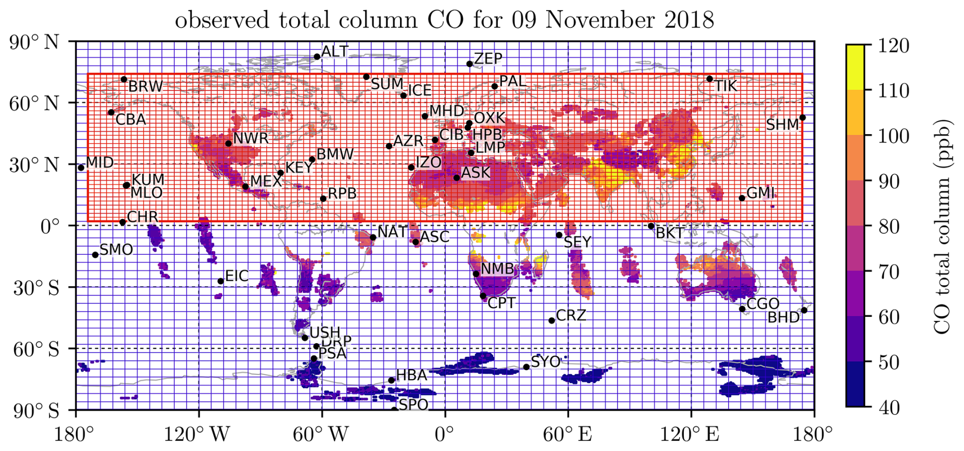
Figure 1 Used zooming setup, with a 6° × 4° grid globally (blue) and nested 3° × 2° grid over the Northern Hemisphere (red). The locations of the background stations where the NOAA CO flask measurements are collected are shown as black dots and labeled with their respective station IDs. The color map shows the used global TROPOMI satellite observations for one day (9 November 2018) as an example of the daily coverage and resolution they provide. Due to strict quality filtering during the retrieval process (Schneising et al., 2023), many places have no valid TROPOMI observations despite every location on Earth being visible to the instrument at least once per day. A more comprehensive overview of the TROPOMI CO data coverage for all of 2018 can be found in Figs. S1 and S2 in the Supplement.

In our inversions, we use the simplified CO-only chemistry version of TM5-4DVAR described in Hooghiemstra et al. (2011), which only explicitly considers the reaction of CO with OH. The OH is prescribed by the widely used monthly climatological fields from the TransCom-CH₄ project described in Patra et al. (2011), in which tropospheric OH is based on the OH fields from Spivakovsky et al. (2000) scaled by 0.92, as suggested in Huijnen et al. (2010). Jiang et al. (2017) show that OH is well buffered in the atmosphere on a global scale over the past few decades, as indicated by the methyl chloroform loss rate varying by only 0.2 % between 2001 and 2015. Thus, the TransCom OH climatology is still considered appropriate for studies investigating recent years. For example, Naus et al. (2022) use it in the context of inverse modeling of CO emissions up to and including the year 2018. In addition to the chemical loss due to OH, CO also experiences loss due to dry deposition, which is simulated using the parameterization from Ganzeveld et al. (1998), adapted for TM5 and ERA-Interim meteorology.

2.2 4DVAR approach

The 4DVAR approach, which was first described and applied to meteorological assimilations by Talagrand and Courtier (1987), has been extended to assimilate atmospheric chemistry by Fisher and Lary (1995) and satellite data by Eskes et al. (1999). While the first applications were strongly limited by computational power, the field flourished recently with rising computational capabilities and more extensive datasets. In the following, a quick rundown on the mathematical basis of the 4DVAR approach is provided based on the more extensive description by Brasseur and Jacob (2017).

The aim of every inversion is to find the state x (here the CO emissions) that fits best the observations y (here the CO columns from TROPOMI and surface flask observations from NOAA). To connect the state x with the observations y, the observational operator F is needed, which includes both the forward model and the spatial and temporal sampling of the observations:

$$\begin{array}{}\text{(1)}& \mathit{y}=\mathbf{F}(\mathit{x},\mathit{p})+{\mathit{\epsilon }}_{\mathrm{O}},\end{array}$$

where p is the model parameter vector, which is every input to F that is not part of the state x (for example meteorology, a priori mixing ratios, or the used chemistry scheme), and ε_O is the observational error, i.e., the combined error of measurements, model, and parameters.

Because ε_O is generally non-zero, there is no single trivial solution for x, that minimizes the difference between the right-hand and left-hand side of Eq. (1). Instead, the state x has to be changed iteratively in a process called optimization. For each state x, a cost J(x) can be defined, which provides information on how well that state fits the observations in a least-squares sense. Additionally, an a priori state x_A is required to regularize the otherwise ill-conditioned problem, preventing non-physical behavior. This “initial guess” can be used to constrain the inversion to reasonable states, for example, by not permitting biomass burning over the oceans. This leads to the cost function

$$\begin{array}{}\text{(2)}& \begin{array}{rl}J\left(\mathit{x}\right)& =(\mathit{x}-{\mathit{x}}_{\mathrm{A}}{)}^{\mathrm{T}}{\mathbf{S}}_{\mathrm{A}}^{-\mathrm{1}}(\mathit{x}-{\mathit{x}}_{\mathrm{A}})\\ & +(\mathit{y}-\mathbf{F}(\mathit{x}\left){)}^{\mathrm{T}}{\mathbf{S}}_{\mathrm{O}}^{-\mathrm{1}}\right(\mathit{y}-\mathbf{F}\left(\mathit{x}\right)),\end{array}\end{array}$$

where S_A and S_O are the a priori and observational error covariance matrices, respectively.

During the optimization process, the model repeatedly runs forward and backward in time. During the forward run, the mixing ratios at times and places of the observations are stored. Based on the stored model mixing ratios and the observations, the cost that corresponds to the current state x can be calculated. During a backward run, the adjoint model, i.e., the adjoint of the tangent linear model, is used. In the case of a linear problem, the tangent linear model is identical to the forward model. This adjoint integration is fed by the mismatches between the forward model and observations (rather than tracer masses) and leads to the gradient of the cost function with respect to state vector element x. Based on that gradient, the state (e.g., the emission fields) for the next iteration cycle is adjusted, which then starts again with a forward run. This cycle is repeated until the gradient of the cost function is sufficiently reduced, i.e., the cost is close to its global minimum.

Overall, in 4DVAR, the model is sampled temporally and spatially for each individual data point, and each point provides its own contribution to the cost function. As such, this approach is well suited to simultaneously assimilate multiple datasets with different spatial and temporal resolutions. One caveat is that the observations of different datasets need to be weighted properly against each other. On the one hand, this implies proper measurement error estimation. On the other hand, some form of error inflation (Sect. 3.2.2) might be required if datasets with vastly different numbers of observations are used or if some datasets have a much higher resolution than the model.

In this study, the inversions are carried out using the non-linear M1QN3 optimizer described in Gilbert and Lemaréchal (1989). This optimizer is capable of handling a semi-exponential description of the probability density function for the a priori emissions, which in turn avoids negative emissions (Bergamaschi et al., 2009). As a convergence criterion, a reduction of the gradient norm of the cost function of 10³ is chosen; i.e., the iterations are stopped once the cost function is 1000 times less steep. This criterion was suggested in Meirink et al. (2008b) to be sufficient to converge the emissions. With this criterion, it takes the model around 35 iterations to converge, whereas the budget terms are near-constant for the last few iterations.

2.3 Model setup

The TM5-4DVAR model, as described in Sect. 2.1, is used to perform multiple inversions of the CO emissions in the year 2018, with a specific focus on the Northern Hemisphere. An overview of settings common across all experiments can be found in Table S1 in the Supplement. All settings are detailed in the following.

2.3.1 Inventories and emission categories

CO production from three distinct source categories – anthropogenic, biomass burning, and secondary CO production through chemistry – is considered. Since the contributions of oceanic and biogenic CO to the overall source are small compared to the aforementioned categories, they have been neglected in this study. Additionally, no daily cycles in emissions or chemistry were considered, mostly due to limitations of the OH climatology (see Sect. 2.1) and the secondary CO production a priori (introduced further down in this section).

As biomass-burning a priori emissions, we use the Fire INventory from NCAR version 2.5 (FINN2.5), which is described in Wiedinmyer et al. (2023) and available at Wiedinmyer and Emmons (2022). FINN is based on three data products from the Moderate-Resolution Imaging Spectroradiometer (MODIS), namely those for active fires, land cover type, and vegetation continuous fields, which are used to infer burned area and fire emissions. Compared to the original FINN version 1 (Wiedinmyer et al., 2011), the FINN version 2 used in this study features an improved representation of large fires by merging overlapping fire pixel areas. Additionally, rather than using a single static vegetation map for all years, the respective MODIS land cover type and vegetation continuous field data from the previous year are used. Also, the fuel loadings and emission factors have been updated. Specifically, we use FINN2.5+VIIRS, which includes additional small-fire detection via satellite observations from the Visible Infrared Imaging Radiometer Suite (VIIRS) and NMVOCs speciated to the Model for OZone And Related chemical Tracers (MOZART-T1) chemical mechanism (Emmons et al., 2020). Naus et al. (2022) found FINN2.5 to be significantly closer to their top-down emission estimates compared to the older FINN1.5.

As a sensitivity study, we conduct additional inversions where we replace FINN2.5+VIIRS as the biomass-burning a priori with (1) FINN2.5 (without VIIRS) and (2) emissions from the Global Fire Emissions Database version 4, including a small-fire boost (GFED4.1s; Randerson et al., 2017). The inversion experiments are introduced in more detail in Sect. 2.3.4.

GFED4.1s is based on satellite observations of burned area from MODIS and fire activity from both the Visible and Infrared Scanner (VIRS) and the Along-Track Scanning Radiometer (ATSR; Giglio et al., 2013). These observations are combined with datasets on vegetation characteristics and meteorology to infer burned area and fire emissions on monthly scales along with scaling factors to receive higher (daily or 3-hourly) temporal resolutions (van der Werf et al., 2017). The small fire boost includes estimates for biomass-burning emissions from fires that are below the detection limit of the burned area product (MODIS) but are still visible as thermal anomalies (Randerson et al., 2012). While these estimates have fairly large errors on a local scale (Zhang et al., 2018), including them leads to more realistic total biomass-burning emissions on the regional to global scale of the model used in this study.

Both GFED and FINN are coarsened to the resolutions of the zooming regions and aggregated into daily bins to serve as global priors for the biomass-burning emissions. After applying the emission factors, all fire types are lumped together into a single biomass-burning fire type. Since both inventories only provide two-dimensional surface level emissions, they are used in conjunction with injection heights from the IS4FIRES integrated monitoring and modeling system for wildland fires developed at FMI (Sofiev et al., 2012, 2013).

For calculating the contribution to the cost function, a grid-scale a priori error of 100 % is assumed globally for the biomass-burning emissions. This error is constructed from the error of at least 50 % provided in van der Werf et al. (2017) for the regional carbon emissions in GFED4.1s, combined with the error of the emission factors that are used to convert the total (carbon) emissions of each fire type into distinct species (e.g., CO). These are fixed per fire type and are reported with an estimate of their natural variability in the order of one-third of the reported value (Akagi et al., 2011). Since GFED4.1s and FINN2.5(+VIIRS) are fairly similar in terms of spatial distribution and amplitude of wildfire emissions (see Fig. S3; note the logarithmic scale) and to keep the inversion results comparable, we assume an a priori error of 100 % for FINN2.5(+VIIRS) as well. Additionally, to prevent erroneous biomass-burning emissions in the inversion result, the a priori error is set to zero over the oceans. While this implies fixed biomass-burning emissions for relatively small islands, for example, Hawai'i, emissions from large islands, for example Indonesia, are still optimized.

TM5-4DVAR allows for spatial and temporal correlations for each emission category to be set. These reduce the effective number of degrees of freedom of the inversion, which can help to prevent overfitting of the observations and lead to more realistic results while also reducing the number of iterations needed to reach convergence (Meirink et al., 2008b). The numeric values for the spatial correlation lengths and temporal correlation times stated in the following are empirical and follow the values provided in Krol et al. (2013), Nechita-Banda et al. (2018), and Naus et al. (2022), who used similar setups and the same model. Biomass-burning events are usually fairly temporary, so a short exponentially decreasing correlation time of 0.1 months for emissions at different times in the same grid cell is used. To account for the usually small spatial extent of biomass-burning events (compared to the coarse resolution of the model grid), we use an exponentially decreasing correlation length of only 200 km for emissions at the same time in neighboring grid cells. The biomass-burning emissions are optimized at a daily resolution in the state (i.e., the optimizer can change the biomass-burning emissions for each day separately, but it cannot change any potential diurnal patterns) to best capture the high temporal frequency of the burning events and therefore maximize the distinction between the biomass-burning emissions and the other categories. Previous studies (e.g., Krol et al., 2013; Nechita-Banda et al., 2018; Naus et al., 2022) used a 3 d resolution in the state (i.e., the optimizer could change the emissions in 3 d chunks but not the relative emission distribution from day to day within each chunk), and in Krol et al. (2013), a sensitivity study with daily resolution was conducted with mixed results.

Secondary CO production from the oxidation of CH₄ and other VOCs is based on three-dimensional production fields from a simulation of the full chemistry model TM5-MP with the extended MOGUNTIA chemical scheme described in Myriokefalitakis et al. (2020) for the year 2018. This source is optimized with a fairly conservative a priori error of only 20 %. We expect fairly gradual changes for this source in time. Therefore, we use an exponentially decreasing correlation time of 9.5 months for the secondary CO production at different times from the same cell. Note that this rather restrictive correlation time does not limit the model's ability to capture the seasonality of short-lived VOCs like isoprene since that seasonality is already included in the prior production fields. Instead, it only limits how much the deviations from those prior fields may vary from month to month. Similarly, spatial emission changes are also expected to be gradual for secondary production, due to the well-mixed CH₄ background, leading to an exponentially decreasing correlation length of 1000 km. A monthly resolution in the state is chosen for the secondary CO production; i.e., the optimizer can change it only once per month, and the production is constant over the course of that month. Choosing this much coarser of a state resolution compared to the daily resolution for biomass-burning emissions, makes it cheaper, with respect to the cost function, for the optimizer to capture the usually short-timescale biomass-burning events with the intended emission category. With all of this combined, the low a priori error, low state resolution, and large temporal and spatial correlation, we hope to reduce aliasing between the smooth fields of this category and the more patchy biomass-burning emissions. Conversely, since NMVOC oxidation can be quite local occasionally, this approach bears the risk of capturing part of the secondary production in the biomass-burning emissions, specifically when the NMVOCs are emitted by fire activity.

Anthropogenic CO emissions are taken from the Climate Model Intercomparison Project 6 (CMIP6) inventory (Eyring et al., 2016), specifically the SSP370 (Fujimori et al., 2017; Riahi et al., 2017; Gidden et al., 2019) projection dataset (Gidden et al., 2018). Due to the low interannual variability of anthropogenic emissions compared to secondary CO production or biomass-burning emissions and the fairly up-to-date inventory (with historical data up to 2014 and projected data from 2015 onwards), a conservative a priori error of 10 % is assumed, with the same monthly state resolution as for the secondary production. Following the same argument as for secondary CO production, we use an exponentially decreasing correlation time of 9.5 months. Similarly, spatial changes in anthropogenic emissions are expected to occur on the level of countries or economic zones, leading to an exponentially decreasing correlation length of 2000 km. As for the biomass-burning emissions, changes to these anthropogenic emissions are restricted to land. Thus, shipping emissions are included in the inventory but not optimized.

2.3.2 Simultaneous inversion of multiple emission categories

As mentioned in the previous section, anthropogenic emissions, biomass-burning emissions, and secondary CO production are optimized simultaneously; i.e., they are all part of the state vector x (Sect. 2.2), and the optimizer could adjust any of them to minimize the cost function. This approach will inadvertently lead to some aliasing between the categories despite the rigid choices for the a priori error, correlation length and time, and state resolution for the secondary production category. However, optimizing the biomass-burning emissions on their own is not an option either since this will force the model to represent any mismatches by adjusting the biomass-burning emissions even if these mismatches actually stemmed from flaws in the chemical production or anthropogenic a priori. This extreme form of aliasing leads to very poor convergence at the background stations even when extremely high a priori errors are assumed. Using not only sparse flask data, but also the high-coverage, high-resolution TROPOMI observations, we might be able to better distinguish between the emission categories.

2.3.3 Initial conditions, spin-up, and main inversions

The initial tracer distribution is an important part of an inversion. Close to the starting date of the inversion period, the initial tracer distribution must fit the total columns and horizontal distribution of the observational datasets reasonably well. If there are significant over- or underestimations, the emission increments will be dominated by the model's efforts to correct for the offset in the mixing ratios. These additional emissions will mask the true signal of the observations, i.e., by how much the a priori emissions differ from the true emissions. In addition, the initial vertical CO distribution must be realistic since the CO depletion and transport vary with altitude. Therefore, assuming too high of an initial mixing ratio in a layer with low transport and low loss will affect the model for a long time. To minimize this type of error, the period of interest (the year 2018) is split into two separate periods, each with separate inversions, and only the second period is considered for the scientific analysis.

During the first period, a spin-up inversion is performed to harmonize the global distribution of CO mixing ratios in the model with the observational datasets (see Sect. 3). This spin-up inversion is started with tracer fields taken from the TM5-MP chemistry transport model, which employed the MOGUNTIA chemistry scheme. See Myriokefalitakis et al. (2020) and references therein for a detailed description of the model, setup, and chemistry scheme, alongside extensive validation against observational data. In addition to the simulation analyzed and described in Myriokefalitakis et al. (2020), the TM5-MP model has been run with the same settings for a longer period, including 2018. Here, we use the instantaneous concentrations from this longer simulation as initial conditions for the spin-up inversion and monthly chemical budget terms for the secondary source of CO from VOC oxidation. The validations in Myriokefalitakis et al. (2020) have shown that the TM5-MP model generally produces reasonably realistic tracer fields in terms of both vertical and horizontal distributions. However, some offsets to the observations still remain. For CO specifically, Myriokefalitakis et al. (2020) found mixing ratios that were too low in the Northern Hemisphere and too high in the Southern Hemisphere. The spin-up inversion in this study is necessary to confidently remove these offsets. In addition, the spin-up inversion facilitates a smooth transition between the different emission datasets used by Myriokefalitakis et al. (2020) in TM5-MP and those used in this study in TM5-4DVAR. The simulations in TM5-MP and in TM5-4DVAR both use CMIP6 for anthropogenic CO and the same meteorology; Myriokefalitakis et al. (2020) also use CMIP6 for biomass burning, while we use FINN2.5 or GFED4.1s. We use different priors for biomass burning because both inventories (FINN2.5 and GFED4.1s) provide historical data rather than projections for 2018, and inversions benefit greatly from realistic lateral a priori distributions that cannot be obtained from projection data as in CMIP6. Another important difference is the treatment of OH. While their OH is calculated online, we use prescribed OH as described in Sect. 2.1. Overall, harmonizing the mixing ratios modeled in TM5-4DVAR and the observations requires that the model is run over a longer period of time. Such a long spin-up period is particularly relevant for high-altitude layers, to which transport through vertical mixing is slow, or regions at large distances from primary sources, to which transport takes a long time. Therefore, the spin-up inversion is run over several months, from 1 January to 1 July 2018.

The second period is the main inversion period, which uses the harmonized mixing ratios from the spin-up inversion as initial conditions. The main inversion period spans 7 months, from 1 June 2018 to 1 January 2019, and leads to the scientifically interesting results presented in Sect. 4. Note that June is part of both the spin-up and the main inversion periods. This overlap is necessary because emissions near the end of each inversion period are verified by very few observations. Therefore, the final month of the spin-up inversion is considered as its spin-down period, during which confidence in the optimized emissions and the resulting mixing ratios is reduced. Similarly, the final month of the main inversions, December 2018, should be considered as their spin-down period. The duration of this spin-down period was chosen based on the lifetime of CO of about 2 months (Raub and McMullen, 1991; Holloway et al., 2000). Hence, a snapshot of the mixing ratios from the final iteration of the spin-up inversion of 1 June 2018 is used as initial conditions for the main inversion. If using these mixing ratios from the spin-up inversion, which are already harmonized to the observations as initial conditions, no further spin-up is required for the main inversions, and their June results can already be trusted.

2.3.4 Experiments

Table 1 gives an overview of the experimental setups for the inversions analyzed in this study. The main inversion period (1 June 2018 to 1 January 2019) is chosen based on the availability of the used input data and computational constraints. Regarding the input data, TROPOMI was in its commissioning phase until March 2018, and the ERA-Interim meteorology dataset ends in August 2019. The latter constraint will be lifted for future studies by switching to ERA5 meteorology (Hersbach et al., 2020). Still, the large zooming region over most of the Northern Hemisphere, which is chosen to gain a deeper insight into the general anthropogenic emission patterns, combined with the long inversion period comes at a high computational cost. Each inversion takes about 5 real-world days to run (even longer with the full-resolution satellite observations). Therefore, the inversion period does not extend into 2019. Emissions for this period are optimized a total of six times with different settings, split into two sets.

Table 1 A priori emissions and observational setup for the conducted experiments. The inflation column lists the error inflation factors as introduced in Sect. 3.2.2.

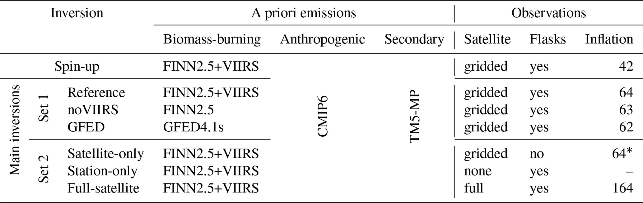
^* The inflation factor for the satellite-only inversion cannot be derived as described in Sect. 3.2.2 since the flask measurements do not contribute to the observational cost in this experiment. Instead, the same inflation factor as for the reference inversion is used to ensure consistent weighting against the prior.

In the first set, we vary the biomass-burning a priori emissions while using the same observations (global gridded TROPOMI observations in conjunction with flask measurements from the NOAA background stations) to constrain the emissions. More details on the a priori emission inventories and the observations used, including the gridding process, can be found in Sects. 2.3.1 and 3, respectively. With these inversions, we intend to investigate the sensitivity of the optimized emissions to the a priori since we introduce a new and updated version of FINN into the model and apply a significantly lower-grid-scale biomass-burning a priori error compared to previous studies. The first set includes (1) the reference inversion with FINN2.5+VIIRS, (2) the noVIIRS inversion with regular FINN2.5, and (3) the GFED inversion with GFED4.1s.

In the second set, the biomass-burning emissions are kept fixed to the reference case (FINN2.5+VIIRS) and the observational datasets are varied. This way, we can assess the information content in the different datasets and the loss of information through gridding. The second set includes (4) the full satellite inversion using the full-resolution satellite data in conjunction with the NOAA surface flasks; (5) the satellite-only inversion using only the gridded satellite observations but no surface flasks; and (6) the station-only inversion using no satellite observations at all, where the inversion is driven solely by the surface flasks.

For the spin-up inversion (1 January to 1 July 2018), we use the same setup as for the reference inversion, i.e., FINN2.5+VIIRS as biomass-burning a priori and gridded satellite observations in conjunction with NOAA surface flasks. All of the main inversions are started from this one spin-up to ensure comparability of the results.

3 Observations

3.1 In situ measurements

The in situ observations used here are the NOAA surface flask CO measurements from various stations assembled by the Carbon Cycle Greenhouse Gases (CCGG) group (Pétron et al., 2020). For filtering out non-background stations, the algorithm described in Hooghiemstra et al. (2012a) is applied to the 54 stations active between January and December 2018. Following this, only the 44 stations shown in Fig. 1 are classified as background and subsequently used. This filtering is necessary to avoid the large representation error introduced by non-background stations. On the one hand, the model has a fairly low-resolution and is not able to capture local sources that might affect the stations. On the other hand, it also has a relatively short time step compared to the weekly or even bi-weekly station measurements, which is why a daily cycle may be caught by the model but not by the stations. Therefore, any station where the model shows a large diurnal cycle is excluded. The criterion is a mean daily standard deviation of more than 3.5 ppb, following the example of Hooghiemstra et al. (2012a). However, background stations and those affected by seasonal biomass-burning signals are kept; in other words, large annual standard deviations are allowed. Using only background stations comes with the implied assumption that air masses reaching them are well mixed, and, therefore, even the coarse resolution of the model (6° × 4°) is sufficient to capture the remaining spatial and temporal variability, allowing for a proper direct comparison of the model to the point observations. To account for any discrepancies from this assumption, the model estimates a representation error for each station based on the slopes (slope scheme introduced in Sect. 2.1) in the box that contains the station.

For the station data, in addition to the representation error of the model, a sampling error of 2 ppb is assumed. This error is composed of the instrument precision of 1.5 ppb given in Gerbig et al. (1999) for the fast-response vacuum UV resonance fluorescence (VURF) CO instrument used at all stations in 2018 and the reproducibility of the measurements of 0.5 ppb provided in the readme file of the dataset (Pétron et al., 2020).

3.2 Satellite observations

The second assimilated dataset consists of the CO total columns from the TROPOspheric Monitoring Instrument (TROPOMI) on board Sentinel-5 Precursor (S5P) satellite launched in October 2017 (Veefkind et al., 2012). TROPOMI provides daily global coverage with a local overpass time at 13:30. The retrieved CO columns also feature a high spatial resolution of up to 7×7 km² at a swath width of 2600 km. Compared to that resolution, even the finest resolution of the model of 1° × 1° might seem very coarse. However, using high-resolution observations not only implies a reduced aggregated observational error if multiple observations are available in a single model grid box, but also gives a chance of at least some cloud-free pixels, i.e., some information, in cloudy model grid boxes.

For this study, we use the TROPOMI/WFMD version 1.8 product from the Carbon and Greenhouse Gas Group at the Institute of Environmental Physics (IUP) of the University of Bremen, retrieved with the weighting function modified differential optical absorption spectroscopy (WFM-DOAS) algorithm, which is described and validated in Schneising et al. (2019, 2023). This retrieval makes use of the TROPOMI observations in the shortwave infrared (SWIR) 2.3 µm spectral range to provide column-averaged dry-air mole fractions of methane and CO. The resulting total columns feature nearly constant sensitivity with respect to altitude. Notably, this includes the troposphere and boundary layer, which is especially useful when investigating biomass-burning events and tropospheric air quality. In addition, observations in the SWIR spectral range, unlike those based on visible light, are capable of seeing through smoke plumes to some degree, making them critically valuable for investigating biomass-burning events. The latter works for smoke but not clouds due to vastly different particle sizes, as demonstrated in Schneising et al. (2020).

As detailed in Schneising et al. (2023), the retrieval employs a fairly strict quality filter, especially with regard to cloudiness, surface brightness, and solar zenith angle (<75°). This selection implies a clear-sky bias in the observations, resulting in an overestimation of photochemical conditions as well as very sparse data over the oceans due to their low albedo. The latter can be seen in Fig. 1, where over the oceans, observations are only possible due to sun glint, which occurs almost exclusively in the center of the orbits (i.e., in a nadir viewing geometry), while the sun is at the zenith. This implies that the sparse observations over the oceans are mostly clustered together.

3.2.1 Gridding

Above, inversions with gridded satellite observations were referenced. To create these so-called super-observations, we follow the approach outlined in Miyazaki et al. (2012). As shown in Fig. 2, for each orbit, we calculate the intersection areas w_i of the footprint of each observation ${\widehat{y}}_i^{\mathrm{o}}$ with the cells of a regular 0.5° × 0.5° grid. We chose this grid resolution based on sensitivity studies conducted in our group (unpublished data), which have shown that at the coarse model resolutions used in this study, inversions based on observations gridded to 0.5° × 0.5° lead to almost the same optimized emissions as those based on the full satellite data, but with a significantly reduced computational cost (using full satellite data entails roughly 25 % longer computation times per iteration). According to Miyazaki et al. (2012), a representative super-observation for each orbit and grid cell can be calculated as an area-weighted average:

$$\begin{array}{}\text{(3)}& {\widehat{y}}_{\mathrm{o}}={\displaystyle \frac{{\sum }_{i=\mathrm{1}}^m{w}_i{\widehat{y}}_i^{\mathrm{o}}}{{\sum }_{i=\mathrm{1}}^m{w}_i}},\end{array}$$

where m observations contribute to this super-observation.

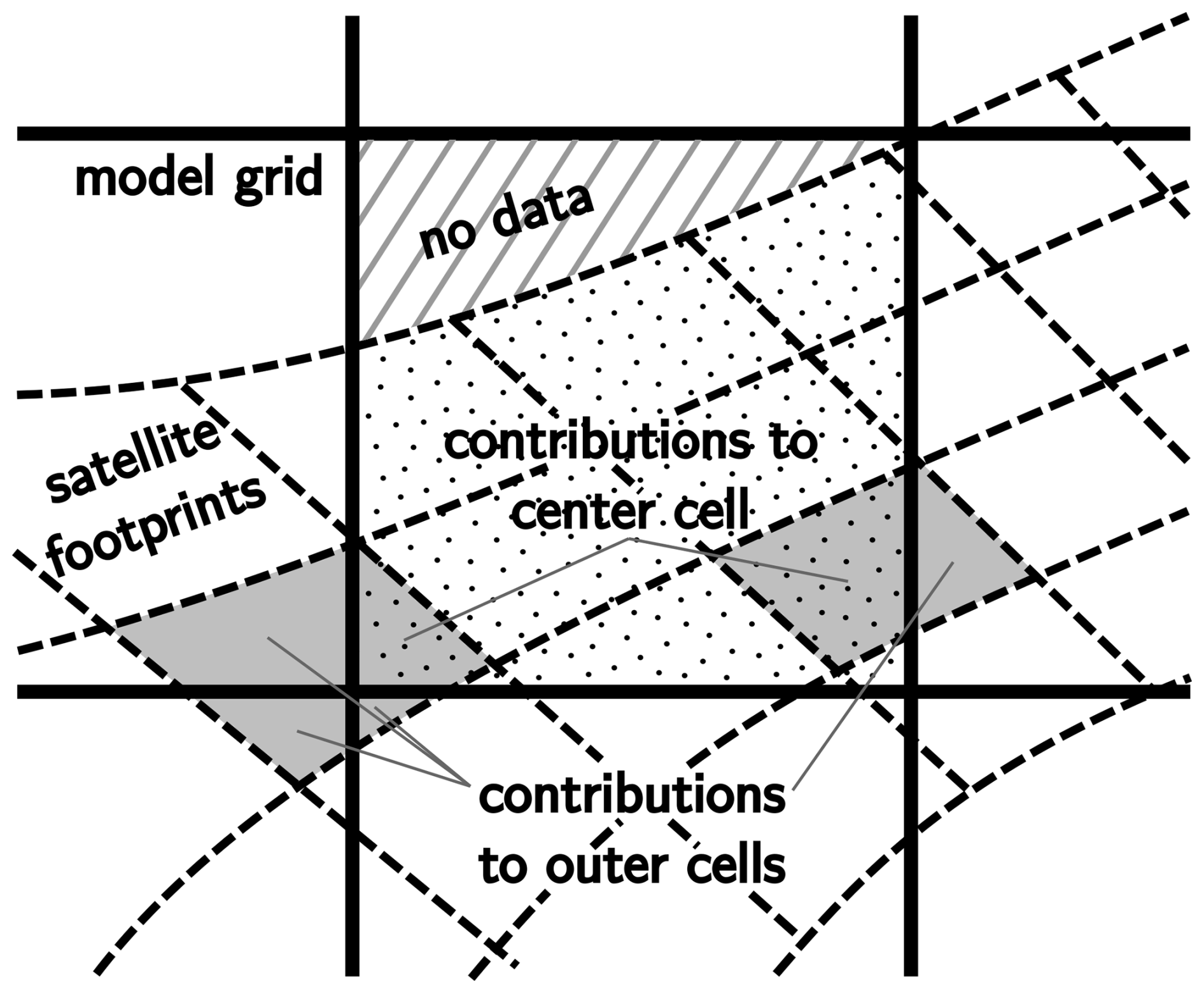
Figure 2 Schematic representation of several satellite footprints (outlined with dashed lines) intersecting with cells of a regular grid (thick, solid lines). The dotted areas show the portion w_i of each footprint that contributes to the center grid cell with area A_cell. For footprints that intersect with more than one grid cell (two examples highlighted in grey), their contributions are further deweighted based on the ratio between their respective intersecting area w_i (i.e., the part that is both dotted and grey) and their total area A_i (the entire grey area). For the striped area, no observations are available; hence, the coverage α for the center cell is <1.

Notably, this average is not weighted by the retrieval error, which stems from the nature of the retrieval, where larger values have larger (absolute) errors, and, therefore, an error-weighted average would be skewed towards low values, as explained in Boersma et al. (2016). The same process of calculating area-weighted averages is also applied to the measurement time, the a priori profile, the pressure levels of the retrieval, and the averaging kernel, level-wise for the latter three.

Unlike Miyazaki et al. (2012), before calculating the super-observation error as an area-weighted average, we first inflate the error corresponding to each individual intersection w_i so that its weight in the cost function (Eq. 2) does not depend on the number of grid cells the corresponding footprint intersects with. This independence can be achieved with a factor $\sqrt{\frac{A_i}{w_i}}$, where A_i is the total area of the satellite pixel's footprint, which contains the ith intersection. The area A_i is equal to w_i if the footprint intersects exactly one grid box. Otherwise, it will be larger, as exemplified in Fig. 2, where the areas A_i, highlighted in grey, are larger than the areas w_i that are simultaneously grey and dotted for the two example footprints. The root stems from the least-squares nature of the cost function, while the rest is simply the inverse of the fraction of the footprint that intersects with the current grid cell. Taken together this yields an area-weighted error:

$$\begin{array}{}\text{(4)}& \mathit{\sigma }={\displaystyle \frac{{\sum }_{i=\mathrm{1}}^m\sqrt{\frac{A_i}{w_i}}{w}_i{\mathit{\sigma }}_i^{\mathrm{o}}}{{\sum }_{i=\mathrm{1}}^m{w}_i}}={\displaystyle \frac{{\sum }_{i=\mathrm{1}}^m\sqrt{A_i{w}_i}{\mathit{\sigma }}_i^{\mathrm{o}}}{{\sum }_{i=\mathrm{1}}^m{w}_i}}.\end{array}$$

Further following Miyazaki et al. (2012), this σ is then deflated by the number n of observations that contribute to the super-observation in that grid cell. However, this deflation is limited by the correlation c between errors of the individual observations (i.e., systematical errors from, e.g., the albedo assumed in the retrieval are correlated in space and do not average out), as suggested in Eskes et al. (2003), and therefore, the super-observation error can be estimated as

$$\begin{array}{}\text{(5)}& {\mathit{\sigma }}_{\mathrm{o}}=\mathit{\sigma }\sqrt{{\displaystyle \frac{\mathrm{1}-c}{n}}+c}.\end{array}$$

Exact values for c are difficult to obtain; however, an upper bound may be found by considering the ratio of the systematic error of the TROPOMI observations versus its random error. From the validations against other observational datasets in Schneising et al. (2023), this ratio can be estimated to be roughly 30 %. As not all systematic error sources from observations within each 0.5° × 0.5° grid box are correlated, c=15 % is assumed here. It should be noted that the exact value of c has nearly no influence on the final inversion results because a larger (smaller) c leads to overall larger (smaller) errors, which, for the most part, are later canceled out by a larger (smaller) error inflation (Sect. 3.2.2).

However, this σ_o does not yet include the representativeness error, which accounts for potential differences between the true average tracer concentration (which includes the parts of the cell that are not covered by observations) and the ${\widehat{y}}_{\mathrm{o}}$ calculated above. For example, if the satellite observes a pristine background in one part of the grid cell, but there is also a plume with high tracer concentrations obscured by clouds in the remaining area, ${\widehat{y}}_{\mathrm{o}}$ is too low. The more of the grid cell area is covered, the smaller this representativeness error becomes.

Miyazaki et al. (2012) suggest a method to estimate this effect. First, the initial mean observation in a cell and the coverage $\mathit{\alpha }=\frac{{\sum }_{i=\mathrm{1}}^m{w}_i}{A_{\mathrm{cell}}},\mathrm{0}\le \mathit{\alpha }\le \mathrm{1}$, where A_cell is the total area of the grid cell, are calculated. In Fig. 2, ${\sum }_{i=\mathrm{1}}^m{w}_i$ is the total dotted area, whereas A_cell is the total cell area enclosed by the thick, solid lines. Next, for well-covered grid cells (α>90 % in Miyazaki et al., 2012), the coverage α is artificially reduced by randomly removing observations. For each observation removed, the mean and coverage of the remaining observations are recalculated. The new mean is then compared to the original value to yield a relative deviation. By repeating this process for many grid cells, a mean relative deviation f_rep(α) can be calculated. Multiplying this relative deviation with the super-observation value ${\widehat{y}}_{\mathrm{o}}$ gives the representativeness error for that cell. In Miyazaki et al. (2012), the mean observations are calculated as a simple arithmetic mean, whereas we use the area-weighted average introduced above:

$$\begin{array}{}\text{(6)}& f_{\mathrm{rep}}\left({\mathit{\alpha }}_k\right)=\left|{\displaystyle \frac{{\widehat{y}}_{\mathrm{o}}-\frac{{\sum }_{l=\mathrm{1}}^{m-k}{w}_l{\widehat{y}}_l^{\mathrm{o}}}{{\sum }_{l=\mathrm{1}}^{m-k}{w}_l}}{{\widehat{y}}_{\mathrm{o}}}}\right|,\mathrm{0}<k<m,\end{array}$$

where k are the removed observations. For the sake of this analysis, we treat the initial observations in each grid cell, i.e., before removing any of them, as if they fully covered the cell. Therefore, ${\mathit{\alpha }}_k=\frac{{\sum }_{l=\mathrm{1}}^{m-k}{w}_l}{{\sum }_{i=\mathrm{1}}^m{w}_i}$ is the coverage compared to the initially covered area rather than the full grid cell area.

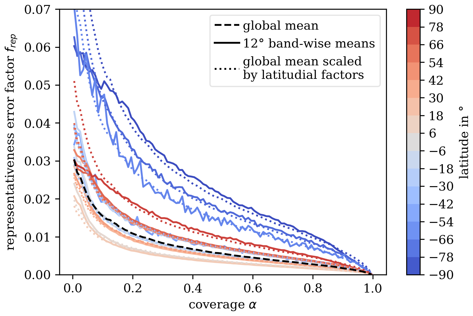
Figure 3 The dashed black line shows the global mean representativeness error factors over the satellite coverage in a given grid cell. This factor is zero for full coverage (α=1) and sharply increases at low coverage values. The colored lines show the mean representativeness error factors over 12° bands. As these are quite noisy, we instead use them to obtain a single scaling factor for each band. These factors are then multiplied onto the global mean representativeness error factors, which leads to the much smoother dotted colored lines.

In this study, to estimate the representativeness error, we analyze 31 d of data, evenly spread over the available observations for 2018. Additionally, we relax the coverage requirement to 50 % to have a larger set of eligible observations, especially when considering coarser grids (not shown in this study). As α_k is a continuous variable, we decided to aggregate it into 1 % bins for the sake of calculating the mean f_rep(α) over the entire analyzed dataset. The resulting global mean representativeness error is shown as the dashed black line in Fig. 3.

We noticed a weak intra-annual variation in the representativeness error factor, with generally slightly larger error values in the Northern Hemispheric summer. However, its magnitude was smaller than the temporal variation on a daily basis. Therefore, we decided to keep the representativeness error fixed in time.

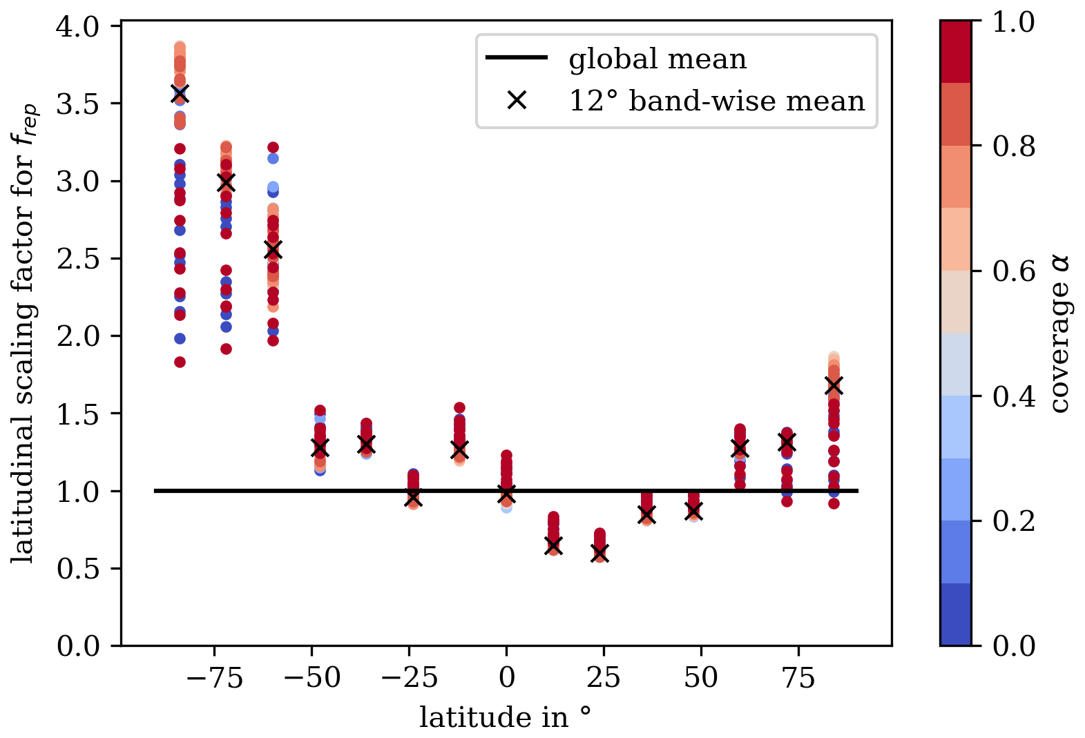
Figure 4 The black crosses are the 12^∘ band-wise scaling factors for the global mean (black line) representativeness error factors, as shown in Fig. 3. Clearly, representativeness errors rise towards the poles, especially in the Southern Hemisphere, where there is less land cover. Additionally, the band-wise scaling factors for each 1 % coverage bin, normalized over the respective global mean for that bin, are shown as colored dots.

In the latitudinal direction, we disregard the very few observations with a center point beyond 89.93° north/south as these might touch and reach beyond the poles, which is problematic for area calculations in the latitude–longitude projection we employ. Additionally, as can be seen exemplified by the colored lines in Fig. 3, there seems to be a strong latitudinal dependence of the representativeness error, with larger values towards the poles and in the Southern Hemisphere. This latitude dependence is likely caused by the poorer measurement quality over the oceans and in high latitudes and smaller grid cell sizes towards the poles. Notably, while the magnitude of the representativeness error increases, the general dependence on the coverage α does not change. To capture this behavior, we additionally average the representativeness error factor over α for each latitudinal 12° band to obtain another scaling factor ${\stackrel{\mathrm{‾}}{f}}_{\mathrm{rep}}\left(\mathit{\varphi }\right)$, with ϕ as the latitude. In Fig. 4, these band-wise factors are plotted before (colored dots) and after (black crosses) averaging over α, all normalized over the global mean. With this, our total representativeness error factor is

$$\begin{array}{}\text{(7)}& f_{\mathrm{rep}}(\mathit{\alpha },\mathit{\varphi })={\stackrel{\mathrm{‾}}{f}}_{\mathrm{rep}}\left(\mathit{\varphi }\right)\cdot f_{\mathrm{rep}}\left(\mathit{\alpha }\right).\end{array}$$

The resulting latitude-wise representativeness error factors are shown as colored dotted lines in Fig. 3. The representativeness error can now be obtained for a given mean observation ${\widehat{y}}_{\mathrm{o}}$, coverage α, and latitude ϕ as

$$\begin{array}{}\text{(8)}& {\mathit{\sigma }}_{\mathrm{r}}=f_{\mathrm{rep}}(\mathit{\alpha },\mathit{\varphi })\cdot {\widehat{y}}_{\mathrm{o}}.\end{array}$$

This leads to the total error of the super-observations

$$\begin{array}{}\text{(9)}& {\mathit{\sigma }}_{\mathrm{s}}=\sqrt{{\mathit{\sigma }}_{\mathrm{o}}^{\mathrm{2}}+{\mathit{\sigma }}_{\mathrm{r}}^{\mathrm{2}}}.\end{array}$$

The super-observations are always assumed to be located at the center of their corresponding cells. This might lead to a spatial bias because observation within an arbitrary grid cell cannot generally be assumed to be evenly distributed.

3.2.2 Error inflation

The uncertainties provided for the individual satellite observations (for the full satellite inversion) and the total error of each of the super-observations (for the inversions that use gridded satellite observations) are inflated with a global factor that depends on the specific inversion setup. For each inversion, this inflation factor is chosen so that the satellite and station observations each make up roughly half of the total observational cost, as suggested in Hooghiemstra et al. (2012a). The intent of this inflation factor is to capture the spatial correlation between the individual satellite footprints and to prevent them from suppressing the signal of the surface stations by their sheer number.

In previous studies, this inflation factor has only been roughly estimated. For example, an empirically chosen variance inflation of 2 was used in Chevallier (2007) for Orbiting Carbon Observatory (OCO) CO₂ observations gridded to 3.75° × 2.5°; an inflation of 50 was used in Hooghiemstra et al. (2012a) and Naus et al. (2022) for MOPITT V4 (gridded to 1° × 1°) and V8 CO observations, respectively; and an inflation of again 50 was used in both Krol et al. (2013) and Nechita-Banda et al. (2018) for IASI CO observations at their native sampling resolution of up to about 25×25 km², with footprints of at least 12 km in diameter. Here, we suggest a more rigorous approach to finding the inflation that fulfills the condition of having each dataset make up an equal part of the observational cost.

Finding the inflation factor at which this condition is fulfilled is in itself an iterative process, where each iteration is a complete inversion. A close look at the cost function (Eq. 2) reveals that for an attempted inflation I, the inflation I^′ for the next iteration can be calculated as

$$\begin{array}{}\text{(10)}& I^{\prime }=\sqrt{{\displaystyle \frac{J_{\mathrm{obs},\mathrm{sat}}}{J_{\mathrm{obs}}-J_{\mathrm{obs},\mathrm{sat}}}}\cdot I^{\mathrm{2}}},\end{array}$$

where J_obs is the total observational cost of the attempt, J_obs,sat is the part of J_obs contributed by the satellite observations, and inflation factors I and I^′ are a factor applied to the observational errors (standard deviations). It should be noted, however, that Eq. (10) will always underestimate the change in inflation needed. For example, if the initial inflation is too large, the formula suggests an improved but still slightly too large of an inflation for the next iteration. This happens because reducing the inflation increases the cost attributed to the satellite observations, which in turn causes the inversion to improve their fit. However, a closer fit to the satellite observations usually implies degradation of the fit to the flask observations, which will increase their contribution to the cost function. That way, the total cost increases and a slightly smaller inflation is needed so that the contribution of the satellite observations makes up half of that cost. In the opposite case, if the inflation is too small, the next guess will be better but still slightly too small.

It may seem that the inflation is solely a parameter of the observational datasets involved and, therefore, fixed for a given set of observations. However, we observed that the inflation also depends on the time of year, the error and temporal resolution of the a priori emissions, and the a priori datasets used. Both a larger a priori error and a higher temporal resolution of the emissions, especially for the biomass-burning emissions, enable the model to fit the satellite observations more easily (lower cost) without degrading the station fit, leading to lower required inflation factors to fulfill the criterion.

With the setup outlined above, we obtained different inflation factors for the individual inversions. Inflation factors are generally larger for the main inversions compared to the spin-up inversion (42). Among the main inversions, we found slight differences based on which of the biomass-burning priors was used. The inflation factors are the largest for the reference inversion (64), followed by the noVIIRS inversion (63), and smallest for the GFED inversion (62), possibly due to smaller a priori mismatches at the stations, as elaborated later. Due to using the same emission setup, the station-only and satellite-only inversions use the same inflation factor as the reference inversion to maintain a similar weight of their background costs to their observational costs and for any analysis steps that require this value to be defined. These (standard deviation) inflation values are larger than the aforementioned variance inflation factors used in Hooghiemstra et al. (2012a) and Naus et al. (2022) for gridded and full-resolution MOPITT observations, respectively, and in Krol et al. (2013) and Nechita-Banda et al. (2018) for full-resolution IASI observations. The larger values are expected because of the higher grid resolution when compared to MOPITT, and the better coverage of TROPOMI when compared to IASI. Due to the much larger number of observations, the largest inflation is required for the full satellite inversion (164). This number is an indication of the higher spatial correlation within the individual observations compared to within the gridded observations since the latter are, by definition, further apart.

The concentrations at the locations of the surface stations depend only relatively weakly on the exact value of the inflation factor because the well-mixed background concentrations show much broader patterns, which are captured by either dataset to some extent. However, very small inflation factors will still cause the station fits to degrade heavily because the satellite data will drown out the flasks. Conversely, for very large inflation factors the model approaches the station-only inversion. This emphasizes the need for the inflation factor to properly weigh both datasets against one another.

However, we concede that there are some issues with the condition of having the observational cost equally distributed between the stations and the satellite observations. This condition implies that satellite observations with higher coverage or lower errors are assigned higher inflation values, i.e., higher-quality data get a lower weight in the cost function. Inadvertently, this leads to overfitting of the surface flasks with increasing quality of the satellite instruments used. Additionally, while we do expect a somewhat larger inflation at higher coverage due to increased correlation between the individual pixels, the current blanket approach of assigning a constant inflation factor to all footprints ignores the actual density and correlation of the observations. This implies that dense observations over the Sahara are inflated just as much as the sparse observations over the oceans. For future studies, this weighting strategy may need to be revised.

4 Results

4.1 Mixing ratio mismatch at the surface stations

4.1.1 Set 1: inversions using different biomass-burning priors

In Fig. 5, the modeled mixing ratios at 6 out of the 44 total ground-level stations are shown before and after the inversions from the first set of experiments (reference, noVIIRS, and GFED), where the biomass-burning inventories were varied. Additionally, the corresponding flask measurement values as well as their assigned uncertainties are indicated. During the spin-up inversion (not pictured), many stations initially exhibit considerable under- or overestimations. The model corrects most of these within the first 1 or 2 months and the mixing ratios at the stations' start to closely follow the observations. This way, during the main inversions (e.g., as shown in Fig. 5), the modeled mixing ratios at all stations are initially close to the observations. At most stations, the mixing ratios simulated based on the optimized emissions remain close to the observations over the whole period of the main inversion. This can be seen, for example, at Mauna Loa (Fig. 5d) and Rapa Nui (Fig. 5f) in the northern and southern Pacific, respectively, and also at stations close to the South Pole, such as Palmer Station in Fig. 5e, despite their very remote nature.

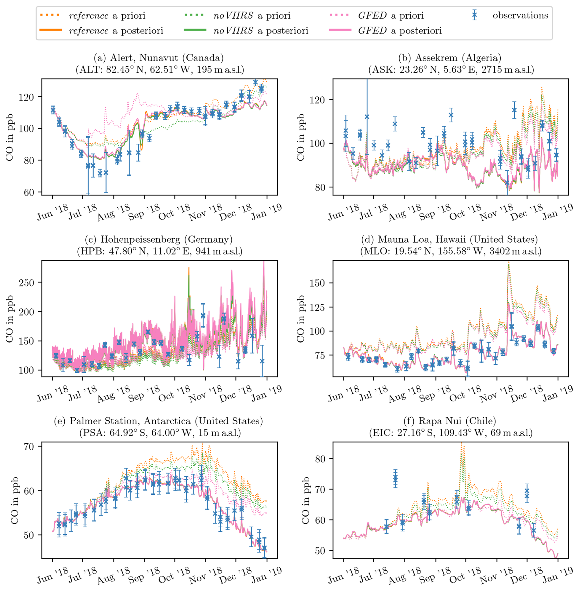
Figure 5 Modeled a priori (dotted lines) and a posteriori (solid lines) mixing ratios sampled at the locations of the stations as well as the flask observations (blue crosses) for six example stations and the three different biomass-burning a priori inventories. For each observation, the corresponding measurement error is indicated as well. Lines are color-coded based on the a priori used: FINN2.5+VIIRS (reference) in orange, FINN2.5 (noVIIRS) in green, and GFED4.1s (GFED) in pink. Unlike the first four, the bottom two stations (e representing PSA and f representing EIC) are in the Southern Hemisphere and, therefore, in the low-resolution global region.

However, at a few stations, the posterior mixing ratios diverge from the measurements to some degree. This effect is mostly limited to high (>55° N) northern latitudes. For example, at Alert, as shown in Fig. 5a, mixing ratios in July and August do not drop far enough, while towards the end of the year, they do not rise high enough. Another problematic station is Assekrem, plotted in Fig. 5b, where the flask observations are systematically underestimated by the model.

Generally, the a priori mixing ratios feature a global accumulation of ground-level CO over time not supported by the observations. This indicates an unbalanced budget, with either sources that are too large (overestimations in the a priori) or a sink that is too small (underestimations in the OH climatology). Given the setup of the inversions, the model resolves this by reducing the emissions in either case. However, there are stations where this does not hold and the a priori underestimates the observations. For example, at Hohenpeissenberg in Fig. 5c, the model finds a fairly strong diurnal cycle and a priori mixing ratios that are generally too low. The former is likely a result of the station being located at the top of a mountain, where upslope conditions cause surface CO to be transported up to the station during the daytime and away during the night. Even though not clearly visible in Fig. 5c, where the full time series is shown, the model is only sampled at the time of the measurement, which would alleviate this issue to some degree. The a priori mixing ratios that are too low, however, could point to the relative proximity of the station to emission sources in central Europe and possibly indicate that the lateral model resolution is not fine enough to properly capture this station.

Table 2 Error-weighted mismatches between observations and model for all main inversions. The first eight rows give the mean mismatches to different subsets of the flask measurements. There, even in the satellite-only inversion, where the flasks did not constrain the emissions, the overall fit at the stations improves, although less compared to the other experiments. The mismatch for the satellite-only inversion decreases significantly if only stations south of 55° N are considered (i.e., excluding ALT, BRW, CBA, ICE, PAL, SUM, TIK, and ZEP), while it stays roughly the same for all other experiments. A considerable portion of the remaining mismatch stems from the stations ASK, HPB, and OXK, where the model generally has problems capturing the observed variability. The last two rows contain the total mismatch to the satellite observations, scaled down by 10³ for readability. Similarly to the satellite-only inversion above, even in the station-only inversion, the overall fit to TROPOMI improves, despite those observations not constraining the inversion.

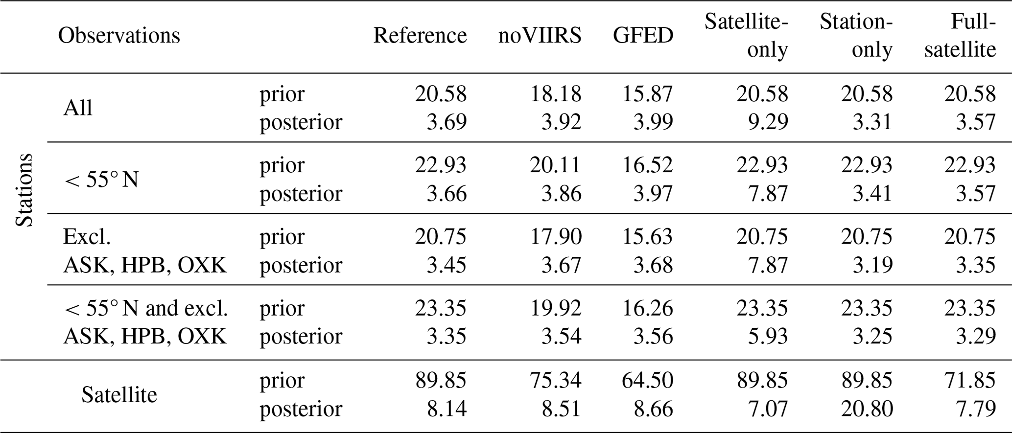
In the first eight rows of Table 2, we calculate the mean error-weighted mismatch ${\stackrel{\mathrm{‾}}{J}}_{\mathrm{flask}}$ between flasks and model for all main inversions, as

$$\begin{array}{}\text{(11)}& {\stackrel{\mathrm{‾}}{J}}_{\mathrm{flask}}\left(\mathit{x}\right)={\displaystyle \frac{{\sum }_{i=\mathrm{1}}^{N_{\mathrm{flask}}}\left[\frac{{\left(y_{\mathrm{flask},i}-\mathbf{F}(\mathit{x}{)}_i\right)}^{\mathrm{2}}}{{\mathit{\epsilon }}_{\mathrm{O},i}^{\mathrm{2}}}\right]}{N_{\mathrm{flask}}}},\end{array}$$

where N_flask is the total number of flask measurements y_flask with observational error ε_O,i and F(x)_i is the model sampled at that measurement. The observational errors include the representation error of the model and the sampling error of the flasks. If the model is capable of capturing the variability of the observations, the unitless quantity ${\stackrel{\mathrm{‾}}{J}}_{\mathrm{flask}}$ should be close to 1. Larger values could point to an underestimated observational error, systematic errors in the model itself, or a model with too few degrees of freedom to capture the variability in the observations, i.e., an underestimated model representation error. When comparing two inversions, lower values represent a better fit. As can be seen for all three experiments of the first set (reference, noVIIRS, and GFED), the fit after the inversion is vastly improved compared to the prior fit. Considering how well the model captures the variability at most stations (e.g., Fig. 5), the a posteriori ${\stackrel{\mathrm{‾}}{J}}_{\mathrm{flask}}$ values of 3 to 4 most likely indicate underestimated errors rather than systematic model errors. Table S2 provides the individual mean error-weighted a priori and a posteriori mismatches for all 44 stations across all six main inversions. The same information is also plotted in Fig. S4, ordered by the latitude of the station.

For most stations, the choice of the biomass-burning a priori has very little influence on the final fit, as evident from the orange, green, and pink lines in Fig. 5 coinciding almost everywhere. Moreover, the a priori mixing ratios from the different inventories themselves are fairly similar. In general, a priori mixing ratios are the lowest before the GFED inversion and the highest before the reference inversion based on FINN2.5+VIIRS, though this does not allow for any conclusions regarding the quality of the inventories. With all three, the a priori mixing ratios are clearly overestimated. While GFED4.1s generates the lowest a priori mixing ratios, which are, therefore, closest to the observations (${\stackrel{\mathrm{‾}}{J}}_{\mathrm{flask}}=\mathrm{15.88}$ is the smallest prior mismatch out of all experiments), this could be coincidental.

4.1.2 Set 2: inversions based on different observational datasets

For the same stations as in Fig. 5, the modeled mixing ratios for the second set of experiments (satellite-only, station-only, and full satellite) based on different observational input datasets are shown in Fig. 6. At the resolution of the model employed in this study, even within the zooming region (up to 3° × 2°), only minor differences in a posteriori mixing ratios are found between the full satellite inversion (green lines) versus the reference inversion (orange lines); i.e., for the sake of this study, those datasets are equivalent. This equivalence is also emphasized by very similar mismatch values in Table 2. In the station-only inversion, where the satellite observations are excluded altogether (brown lines), the fit to the flask measurements gets slightly better (lowest ${\stackrel{\mathrm{‾}}{J}}_{\mathrm{flask}}$ in Table 2), though changes are mostly minimal. Larger changes are found when comparing the former three inversions to the satellite-only inversion (pink lines), in which the model is not driven by the flasks at all. In Table 2, this leads to a significantly larger ${\stackrel{\mathrm{‾}}{J}}_{\mathrm{flask}}$ compared to all the other experiments, yet the mismatch is still lower than for the a priori. This shows that the error inflation factors introduced in Sect. 3.2.2 have been chosen to have meaningful values because the station fits do not significantly degrade due to the satellite observations in the combined inversions.

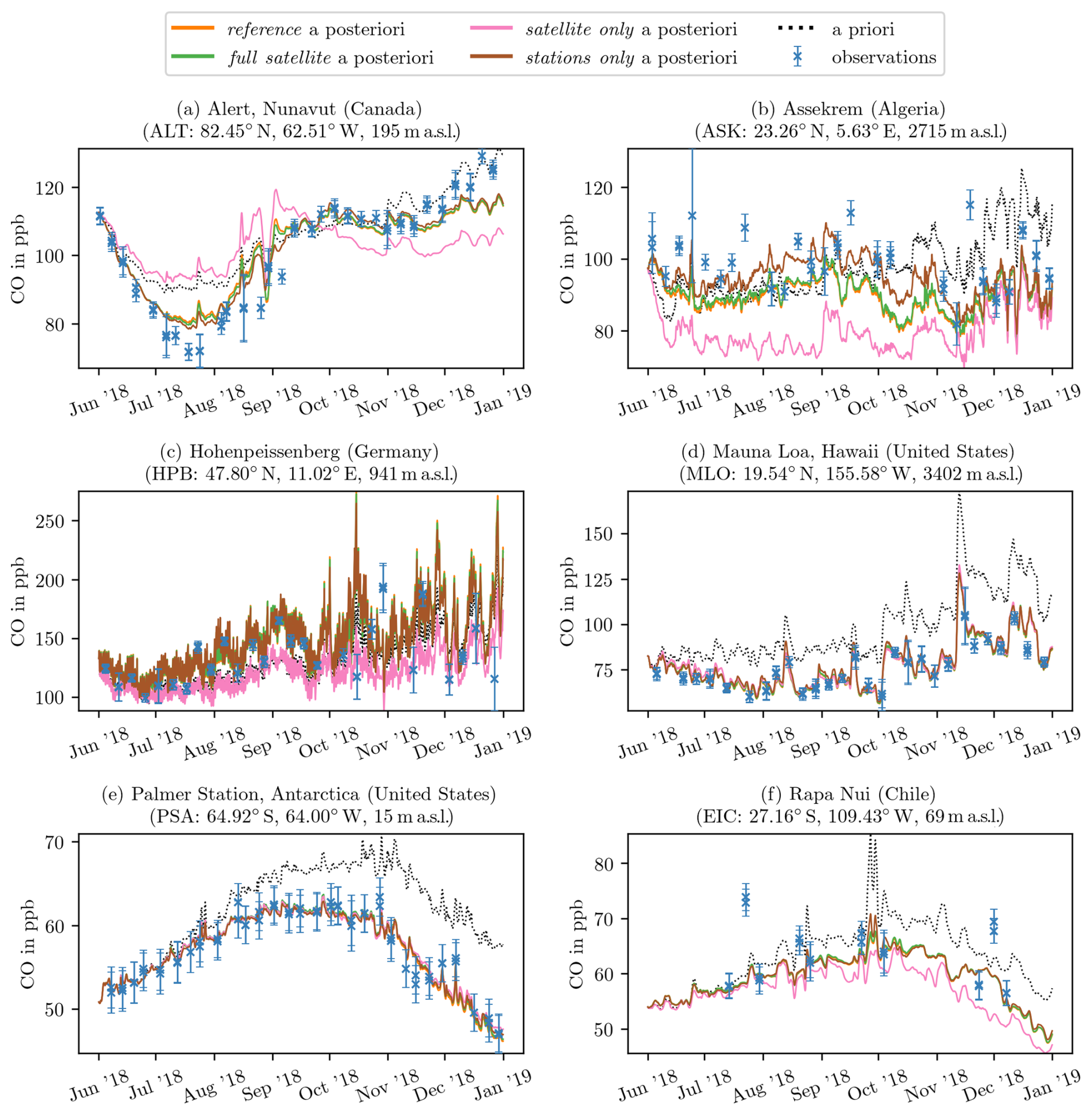
Figure 6 Modeled a priori (dotted line) and a posteriori (solid lines) mixing ratios sampled at the locations of the stations as well as the flask observations (blue crosses) for six example stations and four inversions with different observational datasets. For each observation, the corresponding measurement error is indicated as well. Lines are color-coded based on the observations used: the orange lines represent the reference inversion and are identical to the orange lines from Fig. 5. The full satellite inversion, which also uses a combination of satellite and flask observations, is shown in green. The pink and brown lines represent the satellite-only and station-only inversions, respectively. Note that because all inversions are based on the same a priori emissions, the single dotted black line holds for all four inversions.

Stations at high (>55°) northern latitudes, like Alert in Fig. 6a, exhibit a poor fit quality for the satellite-only inversion. During Northern Hemispheric summer, mixing ratios stay close to the a priori and much higher than the flasks, while in Northern Hemispheric winter, they fall too low, diverging from the a priori and the flasks. This implies that these stations systematically have large mismatches. To illustrate that the fit at other stations is better, we calculated ${\stackrel{\mathrm{‾}}{J}}_{\mathrm{flask}}$ only for stations south of 55° N in the third and fourth row of Table 2. While ${\stackrel{\mathrm{‾}}{J}}_{\mathrm{flask}}$ is significantly reduced for the satellite-only inversion, it stays almost constant for all other experiments. This implies that the satellite observations specifically are insufficient to constrain these stations at high northern latitudes, while the model itself is well capable of capturing them. In the satellite-only inversion, during Northern Hemispheric wintertime, there are very few observations in this region due to little light and high cloud coverage. Therefore, the divergence from the a priori is likely driven by an unbalanced budget in the northern tropical and subtropical regions, where emissions all year round are heavily reduced as shown in Sect. 4.3 below. It is cheaper for the model, in terms of the cost function, to diffuse the decrements over a larger area and shift a part of them to higher northern latitudes than to have even deeper localized decrements in the tropics.

Aside from the northern stations, there are a few other stations that are problematic for the model to capture. The most extreme example of these issues is the station in the Assekrem (ASK) shown in Fig. 6b, where the satellite drives the model to much lower mixing ratios than the flasks. This underestimation can be clearly seen by the very low a posteriori mixing ratios for the satellite-only inversion (pink line) and by the reference inversion (orange line) ending up consistently lower than the station-only inversion (brown line), which is seldom the case for other stations. For this specific station, this effect is likely amplified by its positioning within the Sahara desert, where satellite observations are plentiful due to high albedo and little cloud cover but might also be adversely affected by dust. This oversampling causes the satellite observations to gain a relatively large weight in the cost function compared to the flasks at that location, causing the reference inversion to slightly diverge from the flask observations. Assekrem is also a high-altitude site, which could potentially be problematic with the limited representation of topography in the model. When considering the resulting emission increments (Sect. 4.3), it appears that the model is not capable of capturing this station properly. Another problematic station is Hohenpeissenberg (HPB), shown in Fig. 6c, where the satellite-only inversion, again, suggests much lower mixing ratios. Note the larger range on the vertical axis. Similar, albeit less pronounced results are found for Ochsenkopf station (OXK), which is relatively close to Hohenpeissenberg station geographically. Both are located on mountains at high altitudes. Therefore, as mentioned earlier, the coarse resolution of the model and its limited representation of topography might adversely affect the results there. This misrepresentation will also be further discussed in Sect. 4.3 below, where these specific stations are found to lead to unrealistically high-emission increments, similarly to at Assekrem station. As for the stations at high northern latitudes, these three stations (ASK, HPB, and OXK) degrade the global mean error-weighted mismatch exceptionally strongly. To illustrate this, in the fifth and sixth row of Table 2, we calculate ${\stackrel{\mathrm{‾}}{J}}_{\mathrm{flask}}$ for all but these stations. Again, ${\stackrel{\mathrm{‾}}{J}}_{\mathrm{flask}}$ for the satellite-only inversion is reduced strongly. However, there are also slight decreases for the other experiments, suggesting that the model overall has an issue with properly representing these stations.

Nonetheless, most other stations, regardless of geographical location, show good fits for all four investigated combinations of observational input. As examples for northern tropics, high southern latitudes, and southern tropics, Mauna Loa, Palmer Station, and Rapa Nui, respectively, are shown in Fig. 6d–f. Most notably, the satellite-only inversion manages to closely follow the flask measurements despite them being not assimilated. This can be seen in the seventh and eighth row of Table 2, where both the stations north of 55° N and the problematic stations (ASK, HPB, and OXK) are excluded from the calculation and ${\stackrel{\mathrm{‾}}{J}}_{\mathrm{flask}}$ for the satellite-only inversion gets much closer to the other experiments. These good fits suggest that inversions of current events driven solely by TROPOMI observations are feasible as long as the region of interest is well south of around 55° N.

4.2 Mixing ratio mismatch to the satellite observations

In the final two rows of Table 2, we calculated the total error-weighted mismatch J_sat between satellite observations and model for all main inversions as follows:

$$\begin{array}{}\text{(12)}& J_{\mathrm{sat}}\left(\mathit{x}\right)=\sum _i\left[{\displaystyle \frac{{\left(y_{\mathrm{sat},i}-\mathbf{F}(\mathit{x}{)}_i\right)}^{\mathrm{2}}}{{\mathit{\epsilon }}_{\mathrm{O},i}^{\mathrm{2}}}}\right],\end{array}$$

where y_sat,i is the satellite observations with observational error ε_O,i and F(x)_i is the model sampled at that measurement, with the averaging kernel applied. Figure S5 shows the temporal (monthly) and spatial (12° × 12° grid) distribution of the total error-weighted mismatches for all main inversions. Unlike for the mean error-weighted mismatch ${\stackrel{\mathrm{‾}}{J}}_{\mathrm{flask}}$ between the flasks and the model introduced in the previous section, we do not divide by the number of observations here; hence, we calculate the total instead of the mean mismatch. Considering the total mismatch is necessary because the number of observations in the full satellite inversion is much larger than in all other inversions that use the gridded super-observations. Therefore, the mean error-weighted mismatch for the non-gridded observations is much smaller; i.e., each single observation bears a smaller weight in the inversion. By design, the super-observations have a smaller error than each single observation they are made up of (Sect. 3.2.1), and the error of satellite observations in the full satellite inversion is inflated the strongest (Sect. 3.2.2). Overall, the total mismatch leads to comparable numbers, in this case, while the mean mismatch would not. Again, as for the stations in the previous sections, more detailed data can be found in the Supplement, where Figs. S6 and S7 show the latitudinal distribution of the mean a priori and a posteriori mismatch between the model and the satellite observation in 12° bands for all six main inversions.

Generally, the results are similar to the ones for the stations above. When considering the first set of inversions (reference, noVIIRS, and GFED), the a priori mismatch is again the smallest for GFED and the largest for reference, and for the a posteriori mismatch, this is inverted again. For the second set, the satellite-only inversion results in the best fit to the satellite observations, while the station-only inversion results in the worst. This is akin to the results from the previous section, where the station-only inversion had the best fit to the station data and the satellite-only inversion had the worst fit. As outlined above, the mismatch for the full satellite inversion is special because it is calculated with respect to the non-gridded dataset. Regardless, the mismatch reduction is comparable to the reference inversion.

The mismatches mainly originate from regions known for biomass burning, such as central and southern Africa, northern South America, eastern North America, Indonesia, and Siberia. Even the 0.5° × 0.5° grid of the super-observations is fine compared to the model resolution of 3° × 2° or 6° × 4°. Therefore, any biomass-burning event that leads to steep gradients in the observations cannot be resolved in the model and will lead to mismatches between the modeled and observed mixing ratios.

The global a posteriori mismatches also vary in time and are the largest in August during the height of the burning season. More details on this can be found in Figs. S8 and S9, which show the global total prior and posterior mismatch between the satellite observations and the model for each month of each of the main inversions. This spike in August is especially pronounced in the station-only inversion, where the mismatches already rise in July and slowly taper off over the following months. For this inversion, in addition to the coarse model resolution, the station measurements are too sparse in time and space to properly capture individual biomass-burning events and only constrain the increases in the resulting well-mixed background mixing ratios. Similarly as for the stations, the a priori mismatches are initially low in June and steeply rise over the following 3 months. The good initial fit shows that the spin-up inversion manages to properly harmonize the modeled mixing ratio with the observations as intended. The following rise in mismatches also illustrates the suspected unbalanced budget that causes CO to accumulate in the model.

Figure S10 provides a closer look at the monthly lateral distribution of the total a posteriori mismatch between the satellite observations and the model for each inversion compared to the reference inversion, i.e., when and where each inversion preformed better or worse than the reference inversion. For the first set of inversions, it becomes apparent that, while the GFED inversion leads to worse mismatches overall, the mismatches in Indonesia are slightly smaller compared to the reference inversion. Additionally, noVIIRS and GFED perform slightly better than reference in central Africa in the beginning of the burning season in August to October, but the reference inversion performs better there for the rest of the year.

Further analysis of the second set shows that for the satellite-only inversion the lower mismatch originates mostly from the Northern Hemisphere. Curiously, the mismatch towards the satellite observations around Rapa Nui in the southern Pacific is significantly increased (by roughly 50 %) in the satellite-only inversion for the period from October to December compared to the reference inversion; i.e., in that region, the additional use of flask measurements in the reference inversion leads to a better fit to the satellite observations than using the latter on their own. This apparent contradiction can be resolved by considering that the mixing ratios at such remote locations are, on the one hand, only weakly constrained by the sparse satellite observations over the oceans and, on the other hand, are strongly influenced by transport from distant, land-bound source regions (Daskalakis et al., 2022), which are much more strongly constrained by the satellite observations. The addition of the high-confidence flask measurements from the Rapa Nui station causes the model to diverge from the a priori towards higher emissions around that station, which also better fit the (sparse) satellite observations in that region.

For the station-only inversion, especially large mismatches are observed over northern Africa during the full inversion period. This is most likely related to the issues with the station in the Assekrem outlined in the previous section. During the burning season (July–September), the mismatches in the station-only inversion are the most pronounced over continental Asia, northern and central Africa, northern South America, eastern North America, and the oceans in between those regions. Towards the end of the year, large mismatches are also found around Indonesia. Notably, the station-only inversion shows a degrading fit to the satellite observations in high northern latitudes (>55° N); i.e., the a posteriori mismatch there is worse than the a priori mismatch (see also Fig. S6). This is the only place and time where a degrading fit occurs. As mentioned, all of this behavior is to be expected from the station-only inversion since the sparse station network cannot capture the full spatial and temporal variability of all biomass-burning events globally.

While the mismatches for the full satellite inversion are problematic to compare directly to the other inversions due to the much larger number of observations and the error inflation, the mismatches appear to be smaller in remote regions and larger in active biomass-burning regions compared to the reference inversion. This mismatch distribution is expected because the higher resolution of the full satellite observations implies finer and more pronounced structures from the individual biomass-burning events, which the model can resolve even less effectively than the ones found in the 0.5°×0.5° super-observations.

Interestingly, the mismatches from all main inversions converge in the Southern Hemisphere; i.e., even the station-only inversion fits the satellite observation just as well as the reference or even the satellite-only inversion. This shows that not only is each dataset on its own sufficient to constrain the (remote) Southern Hemisphere, but they also end up at roughly the same result there.

4.3 Optimized global emission fields

4.3.1 Secondary production

Figure 7 provides a global overview of the optimized secondary CO production from VOCs including CH₄ for September 2018 and a comparison to the a priori emissions for the reference inversion. In panels (c) and (d), the absolute and relative differences between the a priori (panel a) and a posteriori (panel b) are shown. For comparison, the relative emission increments for the noVIIRS and GFED inversions can be found in panels (e) and (f), respectively. September was arbitrarily chosen because it is in the center of the inversion period and the results found for the other months are fairly similar. The differences that occur over time are small and limited to variations in amplitude but not in space. This is to be expected, considering the strict temporal correlation times and spatial correlation lengths introduced in Sect. 2.3.1. Figures S11–S13 provide a brief overview of the relative secondary CO increments resulting from the reference inversion for the remaining 6 months of the main inversion period and comparisons of those increments to the ones shown in Fig. 7.

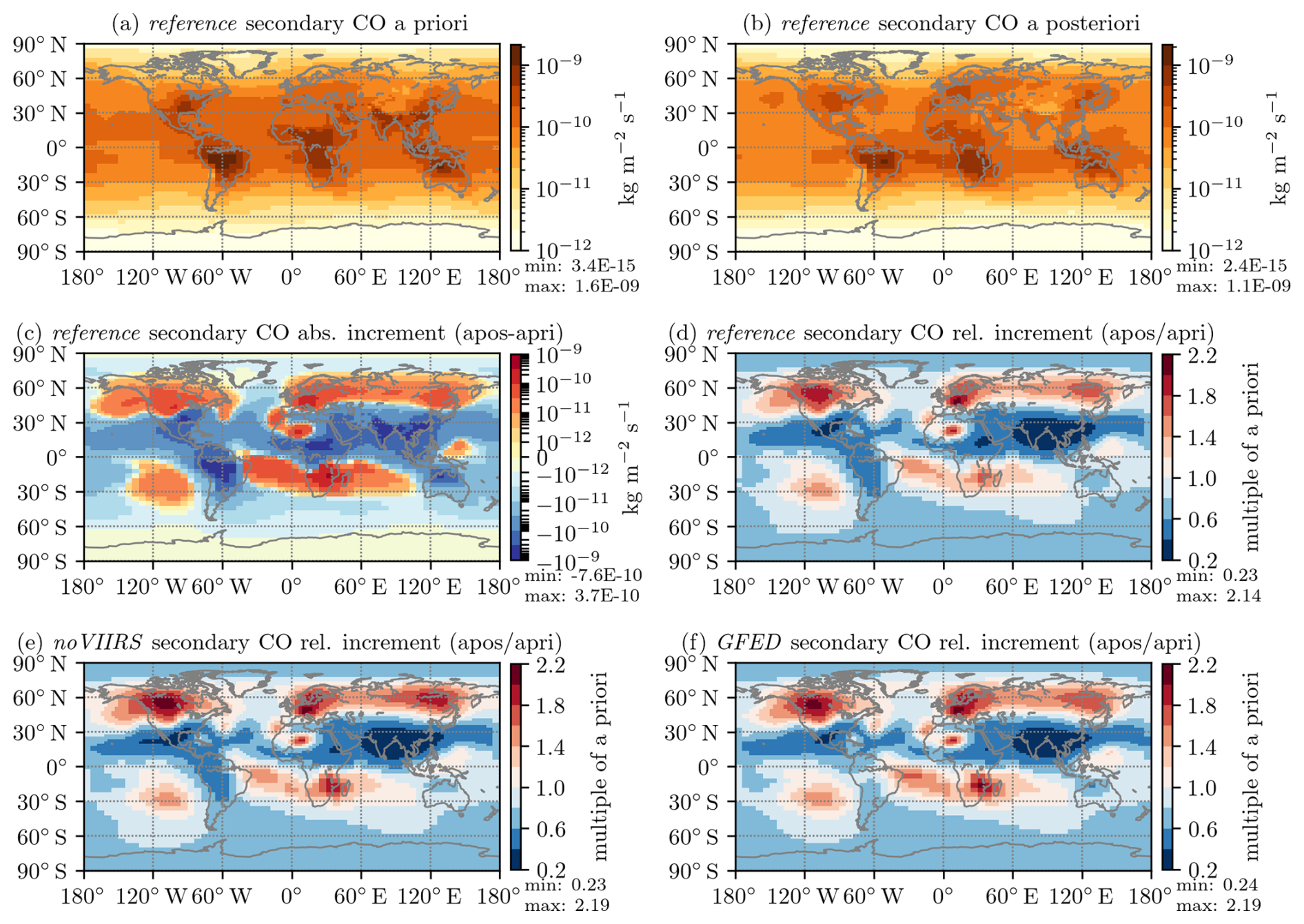
Figure 7 Global secondary CO production for September 2018 for the first set of experiments. The first four panels belong to the reference inversion (based on FINN2.5+VIIRS) and show (a) the a priori emissions, (b) the a posteriori emissions, (c) their absolute difference, and (d) the factor by which the emissions increased. Panels (e) and (f) show this factor for the noVIIRS and GFED inversions, respectively. Note the logarithmic color scales in the first three panels.

All main inversions result in large decrements in a band roughly between the Equator and 40° N. These decrements are especially deep over China and India, as can be seen in the relative increments in Fig. 7d–f. In the later months of the inversion period, this region of large decrements shifts eastwards towards China for all experiments. This northern tropical decrement is analyzed in more detail later on, in Sect. 4.3.2, in the context of anthropogenic emission increments.

The band of decrements is accompanied by increased emissions north of 40° N, especially over central Europe, North America, and Siberia. Additional positive increments can be found between the Equator and 40° S, over the oceans, and in southern Africa. These appear to occur in biomass-burning outflow regions and could point to a systematic error in the lifetime of CO in the model. Due to the band-like structure of the positive and negative increments, this error is possibly caused by inaccurate OH values. Further evidence for such issues with OH values can be found in Myriokefalitakis et al. (2020), where they compare their online calculated OH to the climatological fields from Spivakovsky et al. (2000) used here and find significant differences in those regions. Notably, in the full chemistry simulation, higher OH concentrations imply not only higher CO loss rates, but also higher secondary CO production. Here, we use those production rates paired with loss rates based on the climatological OH, as pointed out in Sect. 2.3.3. Since in our inversions the loss rates are fixed, the model can only compensate for this mismatch by, in some places considerably, changing the secondary CO source.

Table 3 Global prior and posterior budgets for all inversions, as a sum over the global and the zooming regions. The zooming column combines masses going into and coming from the communication cells between the zooming regions. For the main inversions, the 3° × 2° region perceives this as a net loss through advection into these cells, while the global region perceives it as a net gain through emissions within the cells. Only the net effect is shown here. Note that the unit Tg CO yr⁻¹ for the columns showing rates was chosen for ease of comparison to other estimates and does not imply annual rates. The rates were obtained from the processed masses divided by the duration of the respective inversion periods, January to June (6 months) for the spin-up inversion and June to December (7 months) for the main inversions.

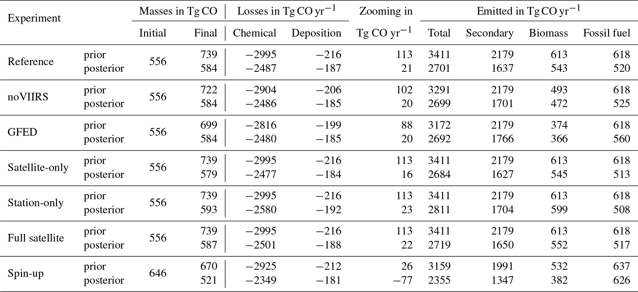
Overall, the a posteriori secondary CO source is lower than the a priori production flux in all experiments, as can be seen in the global budgets provided in Table 3, where the posterior masses at the end of the inversion period (final masses) are consistently lower than the prior final masses. Naus et al. (2022), who used a similar setup, also found too high of a secondary CO production. All fluxes in Table 3 are provided in Tg CO yr⁻¹ despite neither inversion period spanning a full year. While this unit allows for an easy comparison to (annual) budget terms published elsewhere, such a comparison must consider that the inversion period of the main inversions includes the biomass-burning season but excludes the increased anthropogenic emissions due to heating during part of the Northern Hemispheric winter. The biases of such a comparison can be estimated by comparing the prior fluxes from Table 3 for the reference inversion to the respective annual budgets of the prior source estimates, which show an overestimation of around 4 % for biomass burning (FINN2.5) and secondary CO production (from TM5-MP) and underestimation by less than 2 % for the anthropogenic emissions (CMIP6). With this caveat in mind, we compare our prior and posterior budget terms with values from other inversion studies with different setups, namely, to Jiang et al. (2017), who assimilated MOPITT CO and methyl chloroform surface measurements into the GEOS-Chem model, Müller et al. (2018), who assimilated IASI CO in the IMAGES model, and Zheng et al. (2019), who assimilated MOPITT CO in the LMDz-SACS model. A detailed comparison of these three studies can be found in Elguindi et al. (2020). Compared to the results of either of those studies, our a priori budget terms for secondary CO production and chemical loss of CO to OH are far too large. However, our posterior chemical loss falls between the values found in Müller et al. (2018) and Zheng et al. (2019), and our posterior secondary CO production, while still larger, is much closer to what those studies found than our prior. This improved agreement implies that our a posteriori terms are more realistic than the a priori ones. Note that our secondary production implicitly includes ocean and biogenic CO. While the total production and loss terms show reasonably good agreement with the aforementioned studies, the partitioning by source category of our emission terms differs slightly. Our anthropogenic/fossil fuel a posteriori CO is close to that found by Müller et al. (2018) and Jiang et al. (2017) but significantly lower than that reported by Zheng et al. (2019). In contrast, our biomass-burning estimate is close to the multi-year mean of Zheng et al. (2019). However, due to the high year-to-year variability in biomass-burning emissions, as shown by both Müller et al. (2018) and Zheng et al. (2019), this result is difficult to interpret, especially since neither study covers 2018.

As for the stations in Sect. 4.1, the differences in the emission increments between the inversions in the first set (different biomass-burning a priori) are rather small. The most striking differences are the much larger increments (up to 60 % higher final emissions) over southern Africa in both the GFED and noVIIRS inversions (Fig. 7e and f). These are likely related to a known underestimation of African CO emissions in GFED4.1s, as described in Nguyen and Wooster (2020) and references therein. Due to its improved small-fire handling, FINN2.5+VIIRS, as used in the reference inversion, appears to be more capable of capturing those fires. More subtle differences are found in South America, where the GFED inversion only leads to minor corrections (relative increments close to 1), while the reference and noVIIRS inversions show clear decrements (final emissions reduced by up to 50 %). These decrements could be coincidental, considering the importance of OHchemistry and secondary CO production in that region. In the Northern Hemisphere, noVIIRS (Fig. 7e) and GFED (Fig. 7f) feature slightly higher increments over eastern Europe (noVIIRS <10 %, GFED up to 35 %), North America (noVIIRS <10 %, GFED <20 %), and Siberia (noVIIRS <15 %, GFED <5 %) compared to the reference inversion. These differences could point to aliasing of the secondary production emission category to the biomass-burning category. FINN2.5+VIIRS, which is used as the biomass-burning a priori in the reference inversion, has generally the highest emissions, mostly due to capturing small fires, which are common in these regions. For the other two, the model attempts to capture these missing sources, in part, through increasing the emissions in the other categories. Again, this misattribution can also be seen in the budgets in Table 3, where the posterior total emitted mass is very similar for all experiments of the first set, but the distribution over the three emission categories varies considerably.

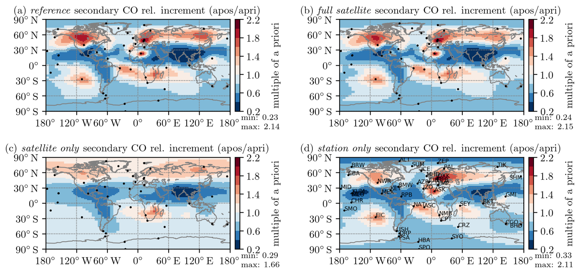
Figure 8 Global secondary CO relative emission increment for September 2018 for the second set of inversions, based on different observational datasets. The panels show the factor by which the emissions increased for (a) the reference inversion, (b) the full satellite inversion, (c) the satellite-only inversion, and (d) the station-only inversion. The locations of the surface stations are indicated with dots for easier orientation in the last panel additionally with their station code. Note that panel (a) of this figure is the same as Fig. 7d.

In Fig. 8, 1 month of the relative increments for the CO production from VOCs and CH₄ is shown for the second set of inversions. Figure 8a is from the reference inversion based on a combination of gridded satellite observations and surface flasks. As such, the content of Fig. 7d above is repeated there for ease of comparison. Very similar results (Fig. 8b) are obtained with the full satellite inversion, as already shown at the surface stations in Sect. 4.1. Minor differences are visible over North America and Siberia, likely due to less aliasing to the biomass-burning category. When the higher-resolution observations are used, the short-term and local biomass-burning events are more distinct, which makes it easier for the model to capture them in the appropriate category.

For the satellite-only inversion (Fig. 8c) many regional features are much less pronounced. However, the broader distribution of emission increments remains the same: There are still negative increments in a band between the Equator and 40° N and over South America and positive increments over southern Africa and the adjacent oceans. The positive increments over North America, Europe, and Siberia are weaker and appear to be spread out over the whole Northern Hemisphere north of around 45° N, including over the oceans. These weaker features are likely linked to the different spatial distributions of observations in the two datasets; while there are many maritime stations and stations in the remote Northern Hemisphere, satellite observations there are more sparse and mostly found in continental regions. Additionally, towards the end of the year, i.e., the second half of the main inversion period, there are no more satellite observations at high northern latitudes, as exemplified in Fig. 1 for one day in early November. All of this, in combination with the spatial correlations given to the optimizer, causes the model to prefer smooth, broad patterns to fill in any gaps.

These differences in information content between the two observational datasets stress the importance of the error inflation (Sect. 3.2.2). If the error on the satellite observations is not inflated, the optimized emissions end up very close to the ones from the satellite-only inversion because the signal from the sparse flask measurements is overshadowed. However, the current inflation may be too large, which causes the optimizer to overfit certain stations that are not well captured by the model. As can be seen in Fig. 8d for the station-only inversion, some stations clearly drive the model away from these broad patterns and towards strong positive regional increments. This overestimation is especially apparent for Assekrem (ASK) and Izana (IZO) stations, which lead to large increments over north-west Africa, and Hohenpeissenberg (HPB) and Ochsenkopf (OXK) stations, which drive emissions over central Europe up strongly. Neither of these increments are observed or supported by the satellite observations. Notably, all of these stations are at high altitudes, potentially pointing to shortcomings in the representation of topography in the model. However, there are mountainous stations, like Mauna Loa (MLO), that are captured well by the model.

Less pronounced examples of overfitted stations are Rapa Nui (EIC) and Tutuila (SMO), which cause positive and negative increments over the southern Pacific, respectively. However, it should be noted that for the satellite, the number of observations over oceans to constrain those emissions is very limited and, as shown for Rapa Nui in Fig. 6f, the satellite-only inversion still manages to fit these stations reasonably well.

Another factor that could play a role in the context of overfitted stations is the strength of the vertical transport in TM5, which Krol et al. (2018) find to be somewhat faster than in other models. This implies low vertical gradients in the troposphere and that modeled tracer mass might be transported upwards before the model can be sampled at the location of the station for comparison to the real observations. This is especially problematic for remote stations with limited surface sources in the vicinity, such as Rapa Nui (EIC) in the south-eastern Pacific. There, the model is forced to introduce unrealistic increments to the secondary CO source in the middle of the Pacific. Furthermore, due to the way those emissions are handled within the model, this introduces additional CO over the whole column (and not only at the surface), which then hampers the comparison to the satellite observations. Similarly, for the station in the Assekrem, in the inversions that include station data, the low vertical gradients cause the optimizer to introduce unrealistically high secondary CO emissions over the Sahara. In contrast, those increments do not occur in the satellite-only inversion because the satellite observes the total column with a very limited vertical resolution and is, therefore, less affected by the vertical gradient in the model.

Finally, even in the station-only inversion (Fig. 8d), some station-driven features appear weaker compared to the reference inversion (Fig. 8a). For example, the positive increments over North America are much weaker, and the spikes around the Assekrem and in central Europe are more spread out. These weaker features are again caused by a combination of the prescribed spatial correlations and the distribution of the available observations. While in the station-only inversion, the model prefers broader patterns to follow the prescribed spatial correlation of the emissions, in the reference inversion, there are satellite observations all around the landlocked stations, which drive the model towards lower increments. Overall, the station-only inversion is driven to the largest emitted mass of all experiments, as shown in the budgets in Table 3. This is in line with the increased emissions around surface stations postulated in the context of the (too) fast (of a) vertical transport in TM5 above.

4.3.2 Anthropogenic emissions

To better identify the aliasing between the emission categories, Fig. 9 provides an overview of the relative increments in the optimized anthropogenic emissions for all six inversions. In Fig. 9a the relative emission increments are shown for the reference inversion based on FINN2.5+VIIRS and a combination of gridded satellite observations and surface flasks. The largest changes are positive increments over Europe and negative increments over China and India. To investigate these increments further, we must first consider that the anthropogenic a priori emissions taken from CMIP6 are projections for 2018 rather than historical data. For China, these projections predict relatively constant emissions. However, China managed to significantly reduce its CO emissions in recent years (Kanaya et al., 2020) in the scope of air quality policies, like the coal-to-gas policy only implemented in 2013 (Liu et al., 2020). Additionally, the effect of most of these policies was somewhat offset by strong biomass-burning years up until 2015 (Zhang et al., 2020), making their effect harder to assess in advance. Regardless, reduced CO concentrations have been now observed all over China, both at surface stations (Liu et al., 2019; Zhai et al., 2019; Li et al., 2020) and from satellites (Zhang et al., 2020). This observed reduction has been linked to a decrease in emissions as calculated using inverse modeling (Zheng et al., 2018). The reduced emissions are most likely due to anthropogenic rather than natural factors (Kang et al., 2019). By 2018, the year of this study, all of this adds up to at least part of the significant offset in CO emissions that we observed. Overall, as shown by Elguindi et al. (2020), bottom-up inventories tend to overestimate recent emissions from China, while the top-down approach leads to more realistic values.

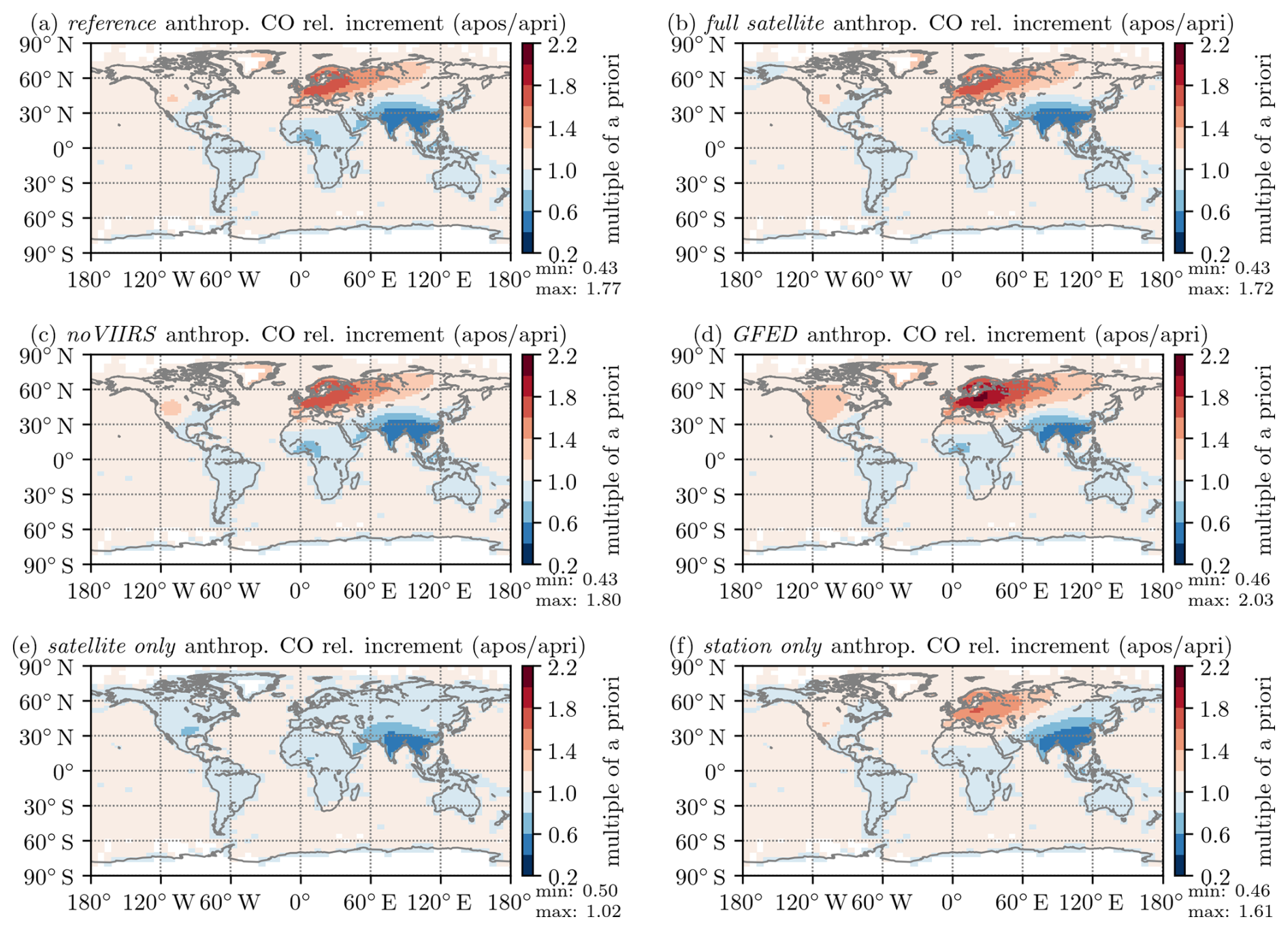
Figure 9 Relative global anthropogenic CO emission increments for September 2018 for all six inversion experiments. Panel (a) shows the reference inversion with FINN2.5+VIIRS as the biomass-burning a priori and gridded satellite observations and surface flasks as observational input. The variations are (b) full satellite observations instead of gridded, (c) noVIIRS with FINN2.5 as the biomass-burning a priori, (d) GFED with GEFED4.1s as the biomass-burning a priori, and (e) satellite-only and (f) station-only increments to drive the inversion.

Unlike for China, there is no clear explanation for the negative increments over India. These might be an artifact due to spatial correlation, where India's proximity to China implies that it is cheaper in terms of the cost function to reduce emissions over a larger region rather than strongly reducing only China's emissions. This could be compounded by low observational coverage, especially with regard to surface stations, and an OH climatology not appropriate for recent years.

When compared to the full satellite inversion shown in Fig. 9b, again, the increments are almost the same, further justifying the usage of gridded satellite observations on a global scale to reduce the computational cost.

The noVIIRS (Fig. 9c) and GFED (Fig. 9d) inversions are slightly worse at capturing the small fires in Europe and North America compared to the reference inversion. The missing small fires lead to apparent anthropogenic increments, especially for GFED, over Europe and western Russia to close the CO budget. Further evidence for this aliasing is provided in Table 3, where the total a posteriori emissions for the inversions of the first set are almost identical, but the partitioning over the emission categories differs significantly. As such, GFED has around 33 % lower biomass-burning emissions compared to the reference but almost 8 % higher both secondary production and anthropogenic emissions.

For the satellite-only inversion, the relative anthropogenic emission increments are pictured in Fig. 9e. They stay relatively close to, but below, 1 globally; i.e., the inversion mostly agrees with the a priori. Over India and China, again, a clear decrement is visible. Notably, there is no increment over Europe in contrast to what we find when flask observations are included. In Sect. 4.1, this smaller increment caused the station at Hohenpeissenberg (Fig. 6c) to be considerably underestimated in the satellite-only inversion.

The station-only inversion shown in Fig. 9f leads to very similar results in terms of anthropogenic increments compared to the reference inversion. This shows how well the NOAA station network on its own is capable of constraining the global broad-scale background emission patterns. Differences include smaller increments over Europe and smaller decrements over Africa and an apparent shift of the decrement over India and China towards the East. The latter may be explained by a lack of background stations and, therefore, a lack of observations in that region, causing the decrement to be smoothed out due to spatial correlation.

Overall, the anthropogenic increments shown in Fig. 9 compared to the ones for the secondary CO production in Figs. 7 and 8 show similar general structures, with decrements in China and India and increments in Europe. However, there are noticeable differences both in finer-scale spatial details; for example, the anthropogenic increments over Europe are more spread out towards eastern Europe, and large-scale patterns, with much smaller relative increments, for North America. Generally, the ratios of a priori to a posteriori emissions, i.e., the relative emission increments, are not the same for all three categories. In other words, while there is some aliasing, the inversion setup is still capable of simultaneously optimizing multiple emission categories, which is ensured in the following ways:

1. Firstly, because of the different a priori errors, even in regions with similar spatial structures, the amplitudes of the relative emission increments differ significantly.

2. Secondly, the different correlation lengths and times for each emission category, as introduced in Sect. 2.3.1, ensure that only the biomass-burning category is capable of capturing short and local events. Conversely, long-lasting, large-scale mismatches could still lead to aliasing across all categories, as is the case, for example, over China.

3. Thirdly, the a priori emissions of all three categories feature different spatial structures.

These a priori structures, combined with enforcing spatial and temporal correlation, imply that it is the cheapest for the model to change emissions following the “spatial signature” of the correct source category rather than evenly distributing the increments over all categories. An example for this can be found over North America, where the anthropogenic emissions are barely changed, while there are significant changes in the secondary CO production.

4.3.3 Biomass burning

An in-depth analysis of the optimized biomass-burning emissions is not included in this study because the low model resolution is not sufficient to capture individual burning events. This promotes aliasing between the emission categories, where the biomass-burning emissions are in- or decreased in large regions co-located with the patterns observed in secondary CO production. As an example of this, Fig. S3 shows the absolute biomass-burning increments for 15 September 2018, the day in the center of the period analyzed above. Because the temporal variability in the secondary CO production is low, the biomass-burning emissions also remain relatively constant in time.

5 Conclusions

We introduced TROPOMI satellite observations into the TM5-4DVAR inverse modeling suit to optimize global CO emissions from three distinct emission categories (biomass burning, anthropogenic, and secondary production) in a set of six inversion experiments. The model ran at a relatively coarse resolution of up to 3° × 2°, which allowed for the use of satellite super-observations gridded to 0.5° × 0.5° to reduce the computational cost. Compared to the inversion based on the full-resolution (up to 7×7 km²) satellite observations, differences in the final mixing ratios and optimized emission fields were minimal. Yet, the computation time per iteration was around 25 % longer for the full-resolution inversion. However, at 3° × 2° resolution, the model could not properly resolve the spatial scale of individual biomass-burning events. This resulted in heavy aliasing of the biomass-burning emissions to the other emission categories. In future studies, using additional observations to further constrain emissions from specific sources or employing a finer zooming region could improve model performance. With the latter, such an inversion could make use of the full potential of the TROPOMI observations.

The comparison between model results and observations is vastly improved by the inversion, and the a posteriori mixing ratios closely follow the observed values. Notably, this even holds true in regions like China and the North Pacific, where the a priori strongly overestimated the mixing ratio and very large emission decrements are required to reach a good a posteriori fit. The overestimated a priori mixing ratios in those regions reveal inconsistencies between the OH climatology used to simulate chemical loss, and the secondary CO production terms taken from the TM5-MP model. This will be further investigated in a study currently in preparation. For the inversion based only on satellite observations, sizable mismatches between model results and flask measurements remain for stations at high northern latitudes. These mismatches can be explained by considering that mixing ratios at high northern latitudes, on the one hand, are poorly constrained by the satellite observations, especially towards the end of the year, and, on the other hand, are governed by transport from the (well-constrained) mid-latitudes, which leaves little leeway for the optimizer. Additionally, in the inversions based on flask measurements, there are very large increments around high-altitude stations. These increments are most likely linked to the coarse model orography that comes with the overall coarse model resolution. Despite good coverage in those regions, the inversion based only on satellite observations neither confirms nor reproduces those strong increments. As such, for future inversions in this framework, an increased model representation error should be applied to those specific stations to avoid biasing results by overfitting.

In the Southern Hemisphere, we find very similar results across all inversions, regardless of the observational dataset(s) (satellite, stations, or both) used. This indicates that, in the Southern Hemisphere, either dataset is equally capable of and sufficient for constraining the background emissions and leads to the same mixing ratios. Potentially, these promising results could allow for inversions based solely on TROPOMI observations, so long as the region of interest is sufficiently far south of 55° N. There, as well as for validation, bias correction, and overall confidence in the optimized emissions, the surface flasks still play a crucial role in the inversion. Using the TROPOMI observations on their own, the long analysis cycle of the surface flasks could be circumvented, and specific events could be investigated using this model in a more timely manner (within weeks rather than months) and only be verified against and adjusted by the flasks at a later stage.

Overall, the most reliable results are found from inversions using both datasets because they complement each other in multiple ways. Firstly, their spatial coverage differs slightly; while the satellite observations are mostly valid over land but sparse over the oceans, most background stations are located on remote islands or in coastal settings. Secondly, both datasets on their own have very limited information on the vertical tracer distribution, where the flasks probe only the surface layer and the satellite observations provide only total column mixing ratios. Combining those datasets can yield better constraints on the vertical tracer distribution in places where in situ and satellite observations are co-located. Finally, in a joint inversion, the satellite observations are implicitly verified versus the flask measurements, and it becomes possible to identify potential biases in the satellite observations. However, when using both datasets at once, the technical limitations of both apply, i.e., the high computational cost from using the satellite observations, and the long analysis cycle of the flask measurements.