Evaluation of dust emission and land surface schemes in predicting a mega Asian dust storm over South Korea using WRF-Chem

This study evaluates the performance of the Weather Research and Forecasting Model coupled with Chemistry (WRF-Chem) in forecasting a mega Asian dust storm (ADS) event that occurred over South Korea on 28–29 March 2021. We specifically evaluated a combination of five dust emission schemes and four land surface schemes, which are crucial for predicting ADSs. Using both in situ and remote sensing data, we assessed surface meteorological and air quality variables, including 2 m temperature, 2 m relative humidity, 10 m wind speed, particulate matter with a diameter of 10µm or less (PM₁₀), and aerosol optical depth (AOD) over South Korea. Our results indicate that prediction of surface meteorological variables is more influenced by the land surface scheme than by the dust emission scheme – generally showing good performance when dust emission schemes are combined with the Noah land surface model with multiple parameterization options (Noah-MP). In contrast, prediction of air quality variables, including PM₁₀ and AOD, is strongly affected by the dust emission schemes, which are directly related to the generation and amount of dust through interaction with surface properties. Among the total of 20 available scheme combinations, the University of Cologne 2004 scheme combined with the Community Land Model version 4.0 (UoC04-CLM4) showed the best performance, closely followed by the University of Cologne 2001 scheme combined with CLM4 (UoC01-CLM4). UoC04-CLM4 outperformed the other scheme combinations by reducing the root mean square errors of PM₁₀ up to 29.6 %. However, both UoC04-CLM4 and UoC01-CLM4 simulated values closest to the MODIS AOD but tended to overestimate the AOD in some regions during the dust emission and transport processes. In contrast, other scheme combinations significantly underestimated the AOD throughout the entire simulation process of ADSs.

1 Introduction

The sand dust storms (SDSs), originating from arid or semi-arid regions, can be lifted to several kilometers and then transported over long distances, sometimes crossing continents (Zhang et al., 2018). They can contain fine particulates, pollutants, and biological materials such as bacteria, viruses, and mold spores (WMO, 2020) – exerting significant impacts on human life and health (Zhang et al., 2016). Therefore, accurate prediction of SDSs is essential to mitigate their impact on public health risks, quality of life, and economic loss.

The SDSs occur in many places around the world, including East Asia (He et al., 2022; Lee et al., 2015; Lee and Lee, 2022), where they are also called Asian dust storms (ADSs); Southwest Asia; the Sahel; the Middle East; and the Mediterranean (Behrooz et al., 2022; Darvishi Boloorani et al., 2021; Su and Fung, 2015; Wu et al., 2016; Yu et al., 2018). In East Asia, the Taklimakan and Gobi Desert account for about 40 % of global dust emissions (Kok et al., 2021). The ADSs occur most often during the spring season (March to May), when surface conditions are dry and wind speeds are strong (Kurosaki and Mikami, 2005; Sun et al., 2001).

Located in East Asia, South Korea is geographically situated within the westerly wind belt; it is predominantly affected by ADSs originating from the Gobi Desert/Inner Mongolia region during the spring season (Lee et al., 2013). The SDSs are also named Hwangsa in Korean, which has the literal meaning of “yellow sands” (Chun et al., 2008; In and Park, 2002; Park and Lee, 2004). It is noted that, among the ADS events that affected South Korea from 2002 to 2021, 82.4 % originated from the Gobi Desert/Inner Mongolia region and 64.7 % occurred in spring (Boo et al., 2022).

The Weather Research and Forecasting Model (WRF) coupled with Chemistry (WRF-Chem; Grell et al., 2005) has been extensively employed for simulating and forecasting the weather and air quality (i.e., trace gases, aerosols, etc.) variables (Chen et al., 2014; Kumar et al., 2014; Liu et al., 2016; Thomas et al., 2019; Wang et al., 2021). Since WRF-Chem incorporates multiple parameterization schemes concerning the planetary boundary layer, land surface, dust emission, radiation, and other physical processes, its performance relies on the combination of parameterization schemes employed in the simulation (Najafpour et al., 2023; Parra, 2023; Rizza et al., 2018; Yuan et al., 2019; Zhao et al., 2020). Therefore, in order to understand the model responses to different parameterization schemes and to enhance the model performance, it is crucial to conduct the sensitivity experiments on the parameterization schemes for the targeted regions and variables.

The SDSs occur when wind speed exceeds a certain threshold value, eroding the soil and releasing dust particles (Chun et al., 2001). In WRF-Chem, the dust emission flux depends on various factors, including soil type, near-surface winds, soil moisture, surface roughness, vegetation, snow, and others within the dust emission scheme (Ginoux et al., 2001; Laurent et al., 2008; LeGrand et al., 2019; Park et al., 2010; Rubinstein et al., 2020; Singh et al., 2017), and they are primarily associated with the land surface scheme in WRF-Chem. For this reason, numerous studies have investigated the sensitivity of different parameterization schemes of the dust emission or land surface processes on simulating SDSs using WRF-Chem.

Yuan et al. (2019) investigated the sensitivity of a severe dust storm that occurred in Central Asia to three different dust emission schemes and showed that the sensitivity results varied across regions, indicating that significant differences in dust emission schemes essentially depend on the sensitivities of threshold friction velocity to surface properties. Najafpour et al. (2023) also examined the accuracy of five different dust emission schemes in estimating dust concentration for a severe SDS in Tehran, Iran; they found that the Global Ozone Chemistry Aerosol Radiation and Transport (GOCART) and Air Force Weather Agency (AFWA) schemes had the best performance compared to the in situ measurements. Zhao et al. (2020) studied the ability of five dust emission schemes to simulate dust emission and transport processes in northwest China; they identified that each of the five schemes had its own strengths and weaknesses, in terms of spatial pattern of dust source region, aerosol optical depth (AOD), aerosol extinction coefficient, and surface PM₁₀ concentrations. Lee and Lee (2022) conducted WRF-Chem simulations by changing the five dust emission schemes for severe wintertime ADS events over South Korea, noting that the University of Cologne 2001 (UoC01) and University of Cologne 2004 (UoC04) schemes were the most successful in simulating severe wintertime Asian dust events while the University of Cologne 2011 (UoC11), GOCART (GO01), and AFWA (GA19) schemes failed to predict them. Rizza et al. (2018) simulated AOD and PM₁₀ for a severe Saharan dust event over southern Italy using three land surface schemes within the WRF-Chem model and reported that the rapid update cycle (RUC) scheme significantly overestimated dust emissions, whereas Noah and the Noah land surface model with multiple parameterization options (Noah-MP) performed better; they demonstrated the impact of the choice of land surface scheme on the prediction of dust emissions. Parra (2023) emphasized the critical importance of accurately representing surface–atmosphere interactions for numerical air quality modeling by conducting sensitivity experiments on four land surface schemes within the WRF-Chem model.

Despite the direct influence of surface properties such as soil moisture, vegetation cover, snow, soil type, and near-surface wind on the dust emission flux, most of these sensitivity experiments focused solely on either dust emission or land surface schemes. Therefore, there were limitations in obtaining the best scheme combination that considers interaction between dust emissions and surface conditions. Furthermore, in the event of severe dust storms deviating from typical conditions, there may be discrepancies in outcomes compared to existing sensitivity studies. Hence, it is necessary to evaluate and propose schemes or combinations through appropriate sensitivity experiments.

In this study, we evaluated the performance of scheme combinations – five for dust emission schemes and four for land surface schemes – for meteorological and air quality variables in a mega ADS event, specifically on 28–29 March 2021.

Section 2 describes the ADS event and methodology, including parameterization schemes in WRF-Chem, and Sect. 3 describes the evaluation results. Conclusions are given in Sect. 4.

2 Methodology

2.1 Mega Asian dust event

Since South Korea is geographically located in the westerly wind zone, it is often affected by the ADSs that occur mainly in the Gobi and Inner Mongolia deserts in spring (March to May) (Lee et al., 2013). Consequently, the government of South Korea introduced the ADS Crisis Warning System (ACWS) in 2015. Additionally, the government and local authorities have prepared for health and safety problems that may arise among the population by utilizing the ADS Response Manual during the occurrence of ADSs.

The ACWS is divided into four-stage crisis warnings – attention, caution, alert, and severe. These stages are determined by the hourly average concentrations of PM₁₀: (1) the attention stage is when hourly average concentrations of PM₁₀ are expected to exceed 150 µg m⁻³; (2) the caution stage is when hourly average concentrations of PM₁₀ are expected to exceed more than 300 µg m⁻³ for longer than 2 h; (3) the alert stage is when hourly average concentrations of PM₁₀ are expected to exceed more than 800 µg m⁻³ for longer than 2 h; and (4) the severe stage is when hourly average concentrations of PM₁₀ are expected to exceed more than 2400 µg m⁻³ for 24 h and then expected to remain at that level for next 24 h, or they are expected to exceed more than 1600 µg m⁻³ for 24 h and then expected to maintain at that level for 48 h. Generally, in South Korea, PM₁₀ concentrations more than 300 µg m⁻³ indicate a high level, whereas those concentrations more than 800 µg m⁻³ are considered a very high level (Boo et al., 2022).

On 29 March 2021, a mega ADS with PM₁₀ concentrations more than 1000 µg m⁻³ was observed in some regions of the Yellow Sea and South Korea. For the first time following the introduction of the ACWS in 2015, the Ministry of Environment of South Korea issued the caution stage warning to 17 cities and provinces nationwide (Kim et al., 2022). Figure 1 shows that the highest PM₁₀ concentration was recorded at 1491 µg m⁻³ at Heuksando, an island located in the Yellow Sea, at 18:00 UTC on 29 March 2021 (03:00 LST on 30 March). During this period, 9 out of 25 Asian dust observation stations from the Korea Meteorological Administration (KMA) exceeded 800 µg m⁻³, indicating a very severe ADS event in South Korea. Based on these findings, we selected this ADS event for this study, which occurred on 29–30 March 2021, and significantly impacted the air quality of South Korea.

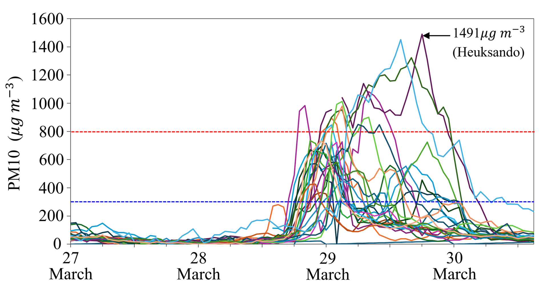
Figure 1 Time series of the hourly averaged PM₁₀ concentrations from 00:00 UTC (09:00 LST) on 27 March to 15:00 UTC on 30 March (00:00 LST on 31 March) at 25 Asian dust observation stations operated by KMA. Colored solid lines represent the PM₁₀ concentrations at each Asian dust observation station. The dashed blue line and dashed red line indicate the threshold values for the ACWS: the caution (≥ 300 µg m⁻³) and alert (≥ 800 µg m⁻³) stage, respectively.

Figure 2 shows surface weather charts associated with the ADS from 26 to 29 March 2021. Here, the source region and site observations of ADSs are identified by the orange-shaded area and red circles, respectively. At 18:00 UTC on 26 March 2021, the ADS originated along the high-pressure-gradient side of a low-pressure system in Mongolia (Fig. 2a). At 12:00 UTC on 27 March, as the low-pressure center moved to eastern Mongolia and Inner Mongolia, the ADS moved to the Gobi Desert/Inner Mongolia (Fig. 2b). At 06:00 UTC on 28 March, the low-pressure center moved toward the north of Manchuria, forming a northwest wind that could carry the sand dusts to South Korea; thus, the ADS moved toward the Bohai Bay, including the Liaodong Peninsula (Fig. 2c). Finally, by 00:00 UTC on 29 March, the ADS affected the entire areas of the Shandong Peninsula and South Korea (Fig. 2d).

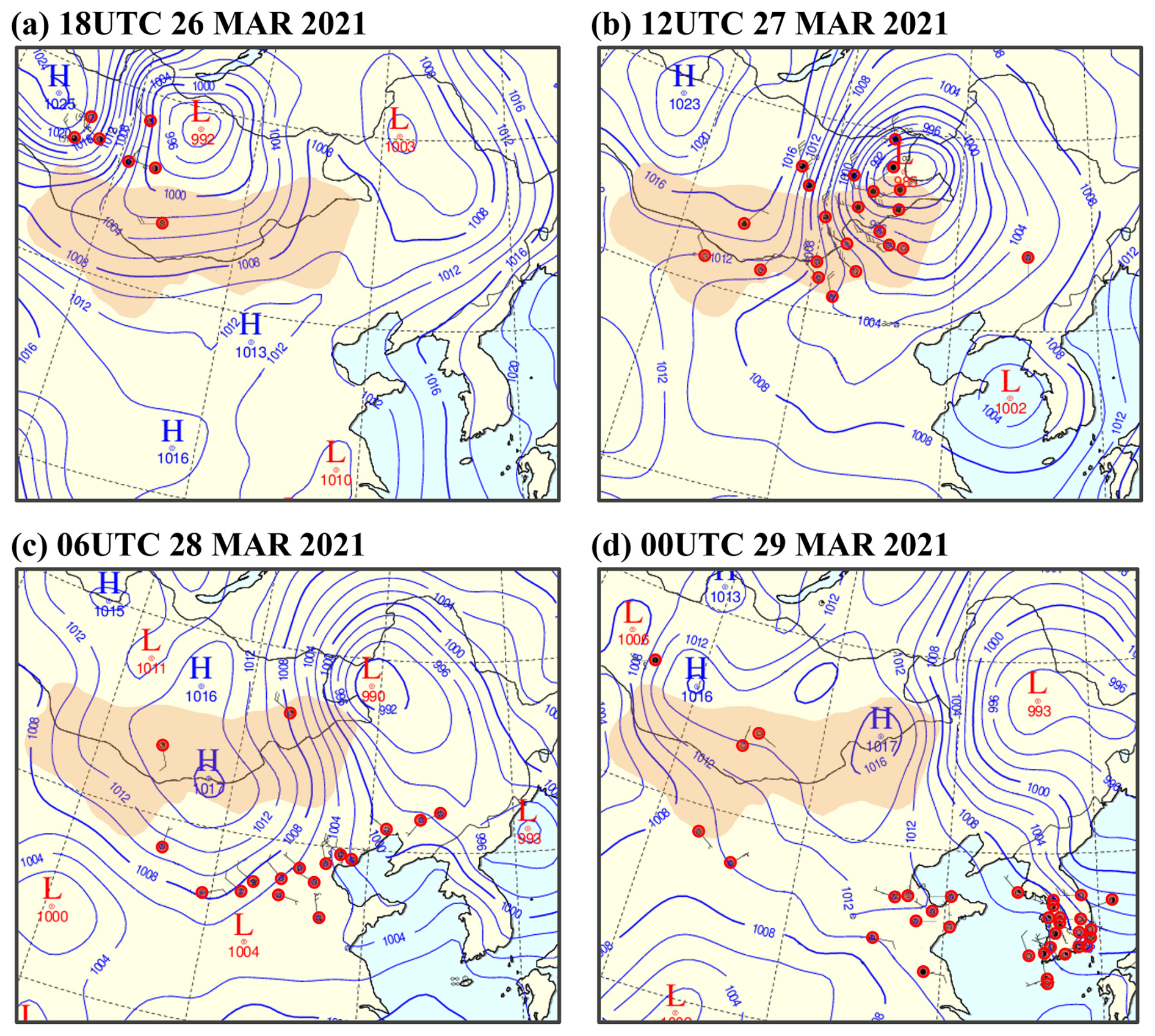
Figure 2 Surface weather charts indicating the source region (orange shading) and site observations (red circles) of the ADS event, along with the sea-level pressure (solid lines; in hPa) for (a) 18:00 UTC on 26 March, (b) 12:00 UTC on 27 March, (c) 06:00 UTC on 28 March, and (d) 00:00 UTC on 29 March 2021. The source region represents the Gobi Desert, including part of Inner Mongolia. Modified from the weather charts by KMA (https://data.kma.go.kr/cmmn/main.do, last access: 14 June 2024).

2.2 WRF-Chem

In this study, we utilized the WRF-Chem model version 4.3.3, a fully coupled meteorology–chemistry model that accounts for interactions between meteorological and chemical processes (Grell et al., 2005). The model domain covers most of East Asia, focusing on the source regions and transport route of ADSs impacting South Korea (see Fig. 3), with a grid spacing of 30 km and 50 vertical levels up to 50 hPa.

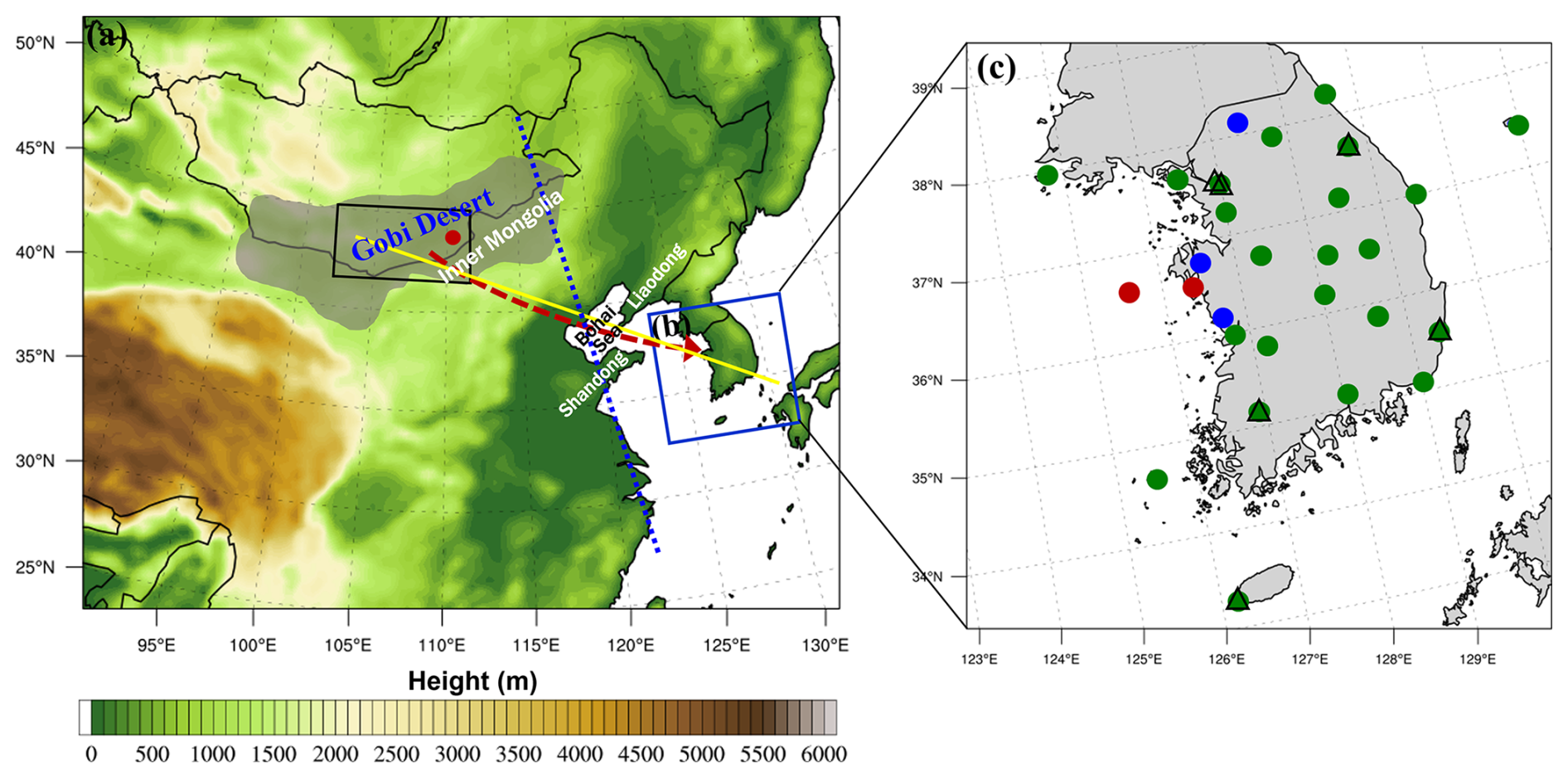
Figure 3 The computational domain with WRF-Chem for (a) simulation; (b) verification against in situ and AErosol RObotic NETwork (AERONET) data in South Korea; and (c) locations of the ASOS, Asian dust observation stations, and AERONET used for verification: in panel (a), the gray shading represents the ADSs source regions for this study case, and the dashed red arrow indicates the main route of ADSs. The solid yellow line denotes the location for vertical cross-section analysis (see Figs. 14 and S11), and the dotted blue line represents the CALIPSO orbit path (see Figs. 13 and S10). In the ADSs source regions, the black square box denotes the area used for verification (see Fig. 10), and the red circle indicates the specific location for additional analysis (see Sect. 3.3). In panel (c), the green circles indicate the locations where the ASOS and Asian dust observation stations coexist – 23 stations; the blue circles represent ASOS stations only – 3 stations; the red circles depict Asian dust observation stations only – 2 stations; and the black triangles indicate AERONET sites – 6 sites.

The meteorological initial and boundary conditions are obtained from the global final analysis (FNL; https://rda.ucar.edu/datasets/ds083.3/dataaccess, last access: 14 June 2024) data set with a resolution of 0.25° × 0.25°, produced by the Global Forecast System (GFS) of the National Centers for Environmental Prediction (NCEP); the boundary conditions are updated every 6 h. The chemical initial and boundary conditions are derived from the Community Atmosphere Model with Chemistry (CAM-chem; https://www.acom.ucar.edu/cam-chem/cam-chem.shtml, last access: 14 June 2024), part of the National Center for Atmospheric Research's (NCAR) Community Earth System Model (CESM), and are produced using the mozbc pre-processing tool (https://www.acom.ucar.edu/wrf-chem/download.shtml, last access: 14 June 2024).

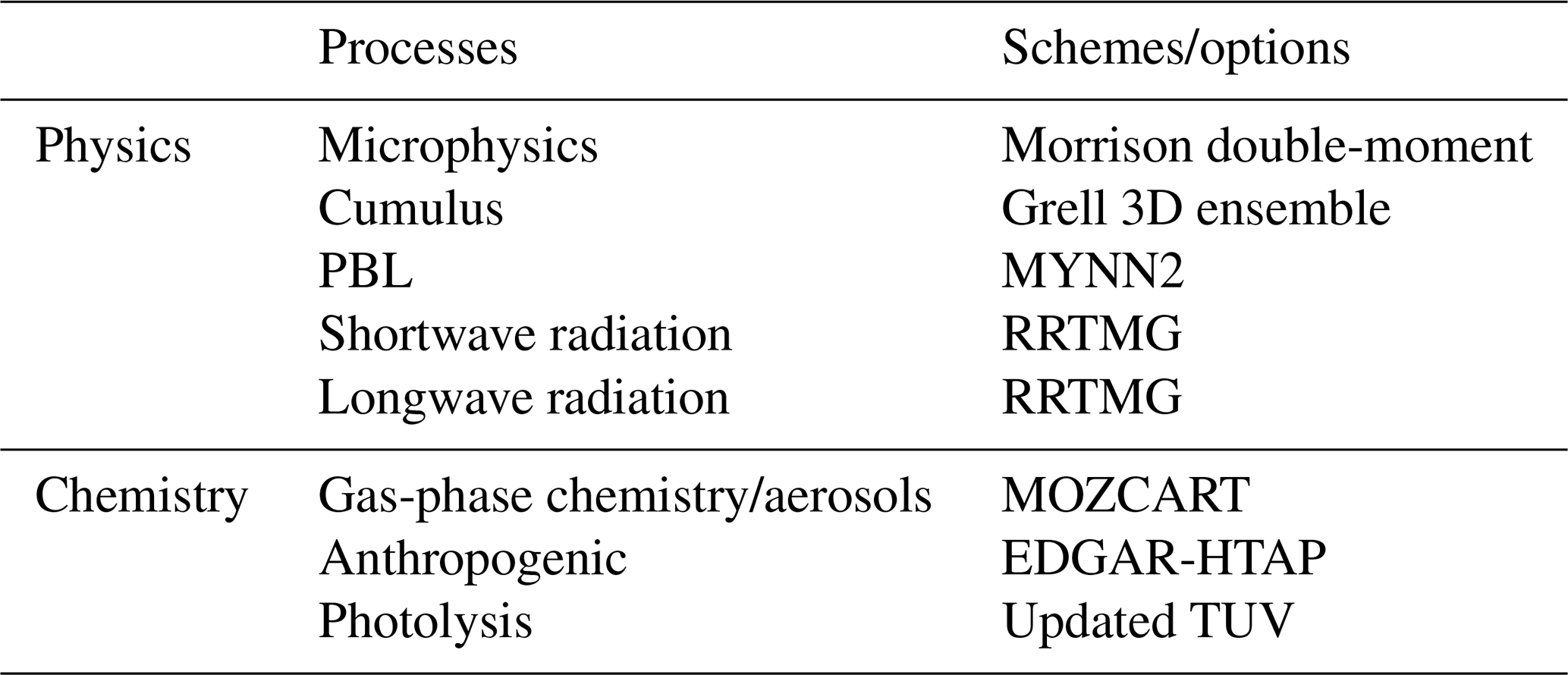
The physical and chemical schemes used in the study, excluding the dust emission and land surface schemes, are detailed in Table 1. The default physics schemes are as follows: Grell 3D ensemble for cumulus parameterization (Grell and Dévényi, 2002), Morrison two-moment scheme for cloud microphysics (Morrison et al., 2009), Mellor–Yamada–Nakanishi–Niino level 2.5 (MYNN2; Nakanishi and Niino, 2006) for planetary boundary layer processes, and the Rapid Radiative Transfer Model for General Circulation Models (RRTMG) for both shortwave and longwave radiation (Iacono et al., 2008). For the chemistry option, MOZCART is selected, which merges the Model for Ozone and Related Chemical Tracers (MOZART) gas-phase chemistry module (Emmons et al., 2010) with the GOCART aerosol module (Chin et al., 2000a, b; Ginoux et al., 2001; Chin et al., 2002). The global emission inventory for anthropogenic emissions is obtained from the Emissions Database for Global Atmospheric Research developed for the Hemispheric Transport of Air Pollutants assessment (EDGAR-HTAP; Janssens-Maenhout et al., 2015), and the updated tropospheric ultraviolet visible (TUV; Madronich et al., 2002) scheme for photolysis is used.

Table 1 The default physical and chemical schemes used in WRF-Chem simulations.

We ran WRF-Chem, including a 72 h spin-up time, from the occurrence of ADSs in the source region until their complete disappearance in South Korea, and the model output was saved at 1 h intervals; therefore, the model run period is from 12:00 UTC on 24 March to 00:00 UTC on 31 March 2021. Note that the 72 h spin-up time is not included in the evaluation process whose performance is calculated every hour and summed up for the total analysis period.

2.3 Dust emission and land surface schemes

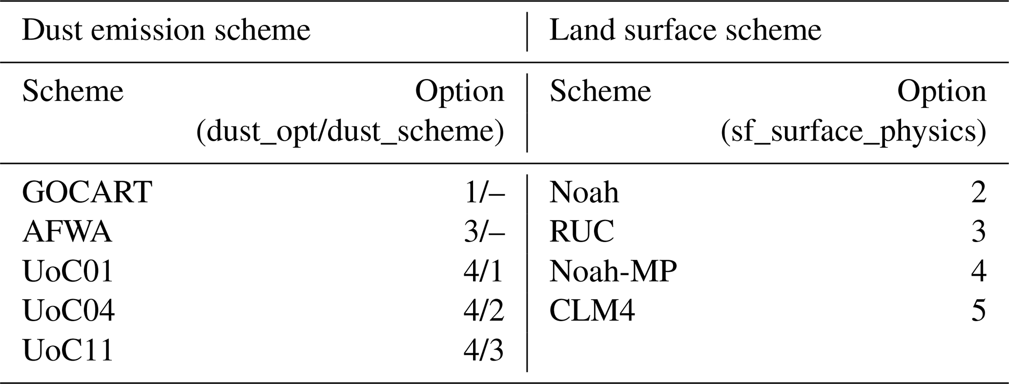
In this study, the sensitivity experiments of scheme combinations are performed for a total of 20 combinations of five dust emission and four land surface schemes in WRF-Chem: the dust emission schemes include GOCART (Ginoux et al., 2001), AFWA (LeGrand et al., 2019), and three versions of University of Cologne schemes – UoC01, UoC4, and UoC11 (Shao, 2001, 2004; Shao et al., 2011); the land surface schemes include the Noah land surface model (Noah; Chen and Dudhia, 2001; Ek et al., 2003), rapid update cycle (RUC; Benjamin et al., 2004), Noah land surface model with multiple parameterization options (Noah-MP; Niu et al., 2011), and Community Land Model version 4.0 (CLM4; Oleson et al., 2010).

Table 2 lists the parameterization schemes used in the above-mentioned description. Hereinafter, in order to distinguish between different scheme combinations, each sensitivity experiment is named in the following format: dust emission scheme–land surface scheme (e.g., GOCART-Noah, GOCART-RUC, AFWA-Noah, etc.).

Table 2 Parameterization schemes of WRF-Chem used for the sensitivity experiments: the dust emission and land surface schemes. The option numbers are the same as in the namelist of WRF-Chem.

2.3.1 Dust emission schemes

The GOCART scheme calculates the dust emission flux based on 10 m wind speed and soil wetness for five bin sizes of dust particles (bin 1: 0.2–2 µm; bin 2:–3.6 µm; bin 3: 3.6–6 µm; bin 4: 6–12 µm; bin 5: 12–20 µm). The dust emission flux at each bin size is estimated as a function of F_p (Ginoux et al., 2001):

$$\begin{array}{}\text{(1)}& F_p=\left\{\begin{array}{l}CS{s}_p{u}_{\mathrm{10}\mathrm{m}}^{\mathrm{2}}\left(u_{\mathrm{10}\mathrm{m}}-u_t\right)\mathrm{if}{u}_{\mathrm{10}\mathrm{m}}>u_t\\ \\ \mathrm{0}\mathrm{otherwise},\end{array}\right.\end{array}$$

where C is an empirical constant (0.8); S is the dust erodibility factor; s_p is the fraction of each bin size class – it is fixed as 0.1 for bin 1 and 0.25 for the other bin sizes; u_10 m is the horizontal wind speed at 10 m height above ground level; and u_t is the threshold velocity, a minimum wind speed at which dust emission can occur, and it depends on particle size and soil wetness.

The AFWA scheme was the updated version based on the Marticorena–Bergametti (MB) dust emission scheme (Marticorena and Bergametti, 1995) in the GOCART scheme (Chin et al., 2000a). It uses friction velocity (u_*) to calculate saltation flux from the surface for a particular dust size as (White, 1979)

$$\begin{array}{}\text{(2)}& H\left(D_{\mathrm{s}}\right)=\left\{\begin{array}{l}\begin{array}{l}C\frac{{\mathit{\rho }}_{\mathrm{a}}}{g}{u}_{*}^{\mathrm{3}}\left(\mathrm{1}+\frac{u_{*t}}{u_{*}}\right)\left(\mathrm{1}-\frac{u_{*t}^{\mathrm{2}}}{u_{*}^{\mathrm{2}}}\right)\\ \end{array}{u}_{*}\ge u_{*t}\\ \mathrm{0}{u}_{*}<u_{*t},\\ \end{array}\right.\end{array}$$

where H(D_s) is the saltation flux; C is an empirical constant (1.0); ρ_a is the air density; g is the gravitational acceleration; u_* is the friction velocity; and u_*t is the threshold friction velocity – a function of particle size, air and soil density, soil moisture, and roughness. The total horizontal saltation flux is calculated as follows:

$$\begin{array}{}\text{(3)}& G=\sum _{s}H\left(D_{\mathrm{s}}\right)\mathrm{d}{S}_{\mathrm{rel}}\left(D_{\mathrm{s}}\right),\end{array}$$

where G is the total horizontal saltation flux considering the sum of each particle size (D_s); s represents nine sand particles that are composed of one clay, five silt, and three sand particles, each defined by specific particle density and effective diameter; and dS_rel is the relative weighting factor for each particle size bin (D_s). The vertical dust flux is then calculated as (Marticorena and Bergametti, 1995)

$$\begin{array}{}\text{(4)}& F_{\mathrm{bulk}}=GS\mathit{\beta },\end{array}$$

where F_bulk is the vertical dust flux – a dust emission flux; S is the erodibility function; and β is the sandblasting efficiency factor (Gillette, 1979) – an empirical function of soil properties (Marticorena and Bergametti, 1995)

UoC01, UoC04, and UoC11 are three versions of dust emission schemes based on Shao (2001), Shao (2004), and Shao et al. (2011), respectively. The latter is further divided into three emission parameterizations with an increasing level of simplification (Shao, 2001, 2004; Shao et al., 2011). The calculation of dust emission flux for UoC01 is as follows:

$$\begin{array}{}\text{(5)}& \begin{array}{rl}& F\left(d_i,d_{\mathrm{s}}\right)=\\ & c_y\left[\left(\mathrm{1}-\mathit{\gamma }\right)+\mathit{\gamma }{\displaystyle \frac{p_{\mathrm{m}}\left(d_i\right)}{p_{\mathrm{f}}\left(d_i\right)}}\right]{\displaystyle \frac{Q_{d_{\mathrm{s}}}g}{u_{*}^{\mathrm{2}}m}}\left({\mathit{\rho }}_b{\mathit{\eta }}_{fi}\mathrm{\Omega }+{\mathit{\eta }}_{ci}m\right),\end{array}\end{array}$$

where F(d_i,d_s) is the vertical dust flux of particle size (d_i) generated by the saltation of particle size (d_s); c_y is a dimensionless coefficient; γ is the weight factor related to dust particle size distribution; p_m(d_i) and p_f(d_i) are the minimally and fully disturbed particle size distribution of the parent soil, respectively; ρ_b is the soil density; m is dust particle mass; Ω is the volume removed by an impacting saltation particle; η_fi is the mass fraction of dust that can be discharged; η_ci is the mass fraction of the aggregated dust; and $Q_{d_{\mathrm{s}}}$ is the saltation flux of particles of size d_s.

The dust emission flux in UoC04 is simplified compared to that in the UoC01 scheme (Shao, 2004). The calculation is as follows:

$$\begin{array}{}\text{(6)}& {\displaystyle }F\left(d_i,d_{\mathrm{s}}\right)=c_y{\mathit{\eta }}_{fi}\left[\left(\mathrm{1}-\mathit{\gamma }\right)+\mathit{\gamma }{\mathit{\sigma }}_p\right]{\displaystyle \frac{Q_{d_{\mathrm{s}}}g}{u_{*}^{\mathrm{2}}}}\left(\mathrm{1}+{\mathit{\sigma }}_m\right),\text{(7)}& {\displaystyle }{\mathit{\sigma }}_p={\displaystyle \frac{p_{\mathrm{m}}\left(d_i\right)}{p_{\mathrm{f}}\left(d_i\right)}},\end{array}$$

where σ_p is the mass ratio of free and aggregated dust and σ_m is the bombardment efficiency.

The UoC11 scheme is further simplified based on the UoC04 scheme. In this scheme, γ is set to 1, and the dust emission flux is determined as follows:

$$\begin{array}{}\text{(8)}& F\left(d_i,d_{\mathrm{s}}\right)=c_y{\mathit{\eta }}_{fi}{\mathit{\sigma }}_p{\displaystyle \frac{Q_{d_{\mathrm{s}}}g}{u_{*}^{\mathrm{2}}}}\left(\mathrm{1}+{\mathit{\sigma }}_m\right).\end{array}$$

2.3.2 Land surface schemes

The Noah scheme assesses soil moisture and temperature in four soil layers with thicknesses of 10, 30, 60, and 100 cm, incorporating vegetation and snow dynamics. It uses equations for soil thermal diffusion and hydrology to determine soil moisture and temperature while accounting for surface energy and water balance. Moreover, it explicitly includes physics related to vegetation and hydrological processes such as evapotranspiration, canopy resistance, surface runoff, soil drainage, albedo, and the influence of urban canopies.

The RUC scheme demonstrates various phases of soil surface water, vegetation effects, and canopy water dynamics; it calculates heat diffusion and moisture transfer through nine soil layers from 0 to 300 cm, with a focus on soil temperature, soil moisture, and snow dynamics (Smirnova et al., 2016). This scheme features a thin surface layer that covers half of the first atmospheric layer and half of the topsoil layer, ensuring accurate representation of the energy budget, and incorporates the components of canopy moisture and soil texture to reflect the effect of vegetation on evaporation.

The Noah-MP scheme is built on the Noah framework but includes updates in physics that encompass dynamic vegetation and ecological processes, as well as snow and underground water processes. This scheme allows flexibility in selecting from multiple options for each physical parameterization. In this study, the default options for each parameterization in the WRF-Chem model are used.

CLM4 is applied in climate studies because of its advanced handling of hydrology, biogeochemistry, biogeophysics, and dynamic vegetation. Its vertical structure consists of a single-layer vegetation canopy, a 10-layer soil column, and a five-layer snowpack (Skamarock et al., 2008). It employs a conceptual Topography-based Hydrological Model (TOPMODEL) to calculate overland flow, focusing on the biogeophysics of the land surface and vegetation dynamics.

2.4 Evaluation data and methods

We evaluated the performance of scheme combinations using three types of data: in situ data, including the Automated Surface Observing System (ASOS) and Asian dust observation data; remote sensing data, including the AErosol RObotic NETwork (AERONET), Cloud-Aerosol Lidar and Infrared Pathfinder Satellite Observations (CALIPSO), and the Moderate Resolution Imaging Spectroradiometer (MODIS); and reanalysis data, including Modern-Era Retrospective analysis for Research and Applications, version 2 (MERRA-2).

2.4.1 Surface observation data

The surface meteorological variables, including 2 m temperature (T2m), 2 m relative humidity (RH2m), 10 m wind speed (WS10m), and surface PM₁₀ concentration, obtained from the ASOS and the Asian dust observation stations (see Fig. 3c) as operated by KMA, were used to evaluate the performance of scheme combinations during the mega ADS event. The T2m and RH2m were utilized as observation data collected at hourly intervals. Due to fluctuations, the WS10m was used as the 10 min average wind speed before each hourly. Since the PM₁₀ concentrations were collected at 5 min intervals, the analysis was conducted using the hourly average concentrations.

2.4.2 Remote sensing data

The AERONET is a global network of ground-based remote sensing aerosol and provides a long-term database of globally distributed aerosol optical properties – AOD, single scattering albedo, and particle size distribution (Holben et al., 1998). In this study, we utilized the Ångström exponent (AE) between 440 and 675 nm and AOD at 500 nm, collected from six sites over South Korea (see Fig. 3c), to calculate the AOD at 550 nm for evaluation. The conversion formula is as follows:

$$\begin{array}{}\text{(9)}& \mathrm{AOD}\left(\mathrm{550}\right)=\mathrm{AOD}\left(\mathrm{500}\right)\times {\left({\displaystyle \frac{\mathrm{550}}{\mathrm{500}}}\right)}^{-\mathit{\alpha }},\end{array}$$

where α indicates AE between 440 and 675 nm, and AOD(500) and AOD(550) represents AOD at 500 and 550 nm, respectively.

The MODIS instruments on the National Aeronautics and Space Administration (NASA) Terra and Aqua satellites observe and monitor Earth's changes with high spatial resolution. They provide near-daily global coverage, allowing the monitoring of various phenomena such as tropospheric aerosols (Kaufman et al., 1997). The MODIS Deep Blue algorithm enables the retrieval of AOD data even over high-albedo surfaces such as deserts and snow-covered areas (Hsu et al., 2006), with a spatial resolution of 10 × 10 km² at 550 nm. In this study, the AOD data retrieved from the Terra Collection 6.1 Level 2 MODIS Deep Blue algorithm (MOD04_L2) are used to assess the time-varying horizontal distribution of simulated AOD by scheme combinations.

CALIPSO carries an aerosol lidar that measures the vertical structure of the atmosphere using an orthogonal polarimeter. It provides aerosol extinction coefficients at 532 and 1064 nm, as well as column AOD data in the troposphere and stratosphere (Vaughan et al., 2004; Winker et al., 2003). In this study, vertical profiles of aerosol extinction coefficients at 532 nm (CAL_LID_L2_05kmAPro-Standard-V4-21; Vaughan et al., 2004) were used to evaluate the vertical structure of modeled dust concentrations.

2.4.3 Reanalysis data

The Modern-Era Retrospective analysis for Research and Applications, version 2 (MERRA-2), represents the latest atmospheric and aerosol reanalysis product from NASA's Global Modeling and Assimilation Office (Gelaro et al., 2017). MERRA-2 is derived from the Goddard Earth Observing System, version 5 (GEOS-5) (Molod et al., 2015; Rienecker et al., 2008), utilizing the GOCART model (Chin et al., 2002) aerosol module (Buchard et al., 2017; Randles et al., 2016), and offers a spatial resolution of 0.5° latitude by 0.625° longitude, with 72 vertical layers from the surface up to 0.01 hPa. MERRA-2 assimilates AOD from a variety of ground-based and remote sensing sources, including the AErosol RObotic NETwork (AERONET; 1999–2014), Advanced Very High Resolution Radiometer (AVHRR), Multiangle Imaging SpectroRadiometer (MISR; 2000–2014), and MODIS on both Terra (2000–present) and Aqua (2002–present) satellites (Buchard et al., 2017; Gelaro et al., 2017). In this study, MERRA-2 is employed to compare the AOD spatial distribution with AOD simulated by various scheme combinations.

2.4.4 Evaluation metrics

In this study, the simulated surface meteorological variables and PM₁₀ concentrations were compared with observation data using two types of evaluation methods: (1) using the difference between predicted and observed values – Pearson's correlation coefficient (PCC) represents the level of linear relationship between the forecasts and observations, the mean bias error (MBE) is the arithmetic average of the differences between forecasts and observations, and the root mean square error (RMSE) estimates the average error of the model and uses the square of the difference between the forecasts and observations; (2) determining detection success using an arbitrary threshold (categorical metrics) – this method requires a threshold for binary classification using a 2 × 2 contingency table (see Table 3) and was applied for only PM₁₀ evaluations in this study.

Table 3 Contingency table for forecast evaluation: this table categorizes the outcomes of forecasts versus actual observations into four distinct types – hit (a), when both the forecast and observation agree on the event occurring; false alarm (b), when the forecast predicts an event that does not occur; miss (c), when an event occurs but is not forecasted; and correct rejection (d), when neither the forecast nor the observation indicates the occurrence of an event.

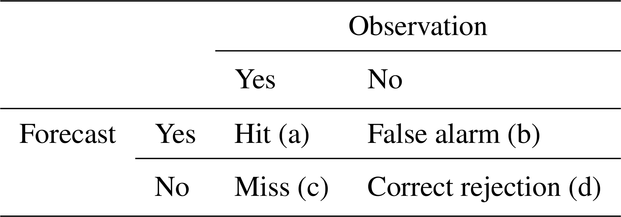
For categorical metrics, we considered the threshold values of the fine dust alert and ACWS provided by the Atmospheric Environment Administration of South Korea – the threshold values are 80 µg m⁻³ (poor air quality due to fine dust), 150 µg m⁻³ (very poor air quality due to fine dust; attention), 300 µg m⁻³ (caution), and 800 µg m⁻³ (alert), respectively. In Table 3, “hit” and “correct rejection” indicate accurate predictions, whereas “false alarm” and “miss” suggest inaccurate predictions. The probability of detection (POD) evaluates the ratio of accurate forecasts to observed events, indicating how often an event is predicted correctly when it occurs. It ranges from 0 to 1, with 1 indicating a skillful forecast and below 0.5 indicating poor performance. Note that POD does not account for events without observed events, which means that an increased tendency to overestimate the frequency of events can lead to an artificial improvement in performance. The false-alarm rate (FAR) is utilized to assess the ratio of false alarms to events, predicting an event when it is not observed. FAR also ranges between 0 and 1, where values closer to 0 indicate better forecast skill. In contrast to POD, since FAR does consider events without observed events, an increased tendency to underestimate the frequency of non-events can result in an artificial skill improvement. Therefore, it is essential to consider FAR with POD to address these limitations. Additionally, the critical success index (CSI) is an important metric used to evaluate the overall accuracy of forecasts. It measures the ratio of correctly forecast events to the total number of observed and forecast events, accounting for both “false alarm” and “miss” events. In other words, CSI addresses the limitations of POD and FAR by integrating both metrics, providing a clearer assessment of overall forecast performance. The CSI value ranges from 0 to 1, with values closer to 1 indicating higher forecast skill. CSI is particularly useful because it considers both over-forecasting and under-forecasting, showing how accurate the forecast is. The formulas for POD, FAR, and CSI are as follows:

$$\begin{array}{}\text{(10)}& {\displaystyle }\mathrm{POD}={\displaystyle \frac{a}{a+c}},\text{(11)}& {\displaystyle }\mathrm{FAR}={\displaystyle \frac{b}{b+d}},\text{(12)}& {\displaystyle }\mathrm{CSI}={\displaystyle \frac{a}{a+b+c}}.\end{array}$$

3 Results

3.1 Evaluation using in situ data

The verification against the in situ data (i.e., ASOS and Asian dust observation stations) is conducted for T2m, RH2m, WS10m, and surface PM₁₀ concentrations at the given observational stations in South Korea. The values are averaged over the stations (see the station locations in Fig. 3c).

3.1.1 Surface meteorological variables

Figure 4 shows PCC for all scheme combinations. Since surface meteorological variables are primarily influenced by the land surface scheme, the performance differences caused by the dust emission schemes were very small in the validation results. The scheme combinations generally have good correlation with high to moderate PCCs for surface meteorological variables: 0.73–0.77 for T2m, 0.73–0.77 for RH2m, and 0.58–0.62 for WS10m (Fig. 4). More details are as follows: (1) for T2m, the highest correlation is achieved by scheme combinations based on Noah-MP (0.77), followed by CLM4 (0.74–0.75), Noah (0.74), and RUC (0.72–0.73) (Fig. 4a); (2) for RH2m, the highest correlation is also shown by combinations based on Noah-MP (0.77), followed by CLM4 (0.74–0.75), Noah (0.74–0.75), and RUC (0.72–0.73) (Fig. 4b); and (3) for WS10m, a similar correlation is achieved by scheme combinations based on Noah-MP (0.61–0.62), RUC (0.61–0.62), and CLM4 (0.61), followed by Noah (0.58–0.60) (Fig. 4c).

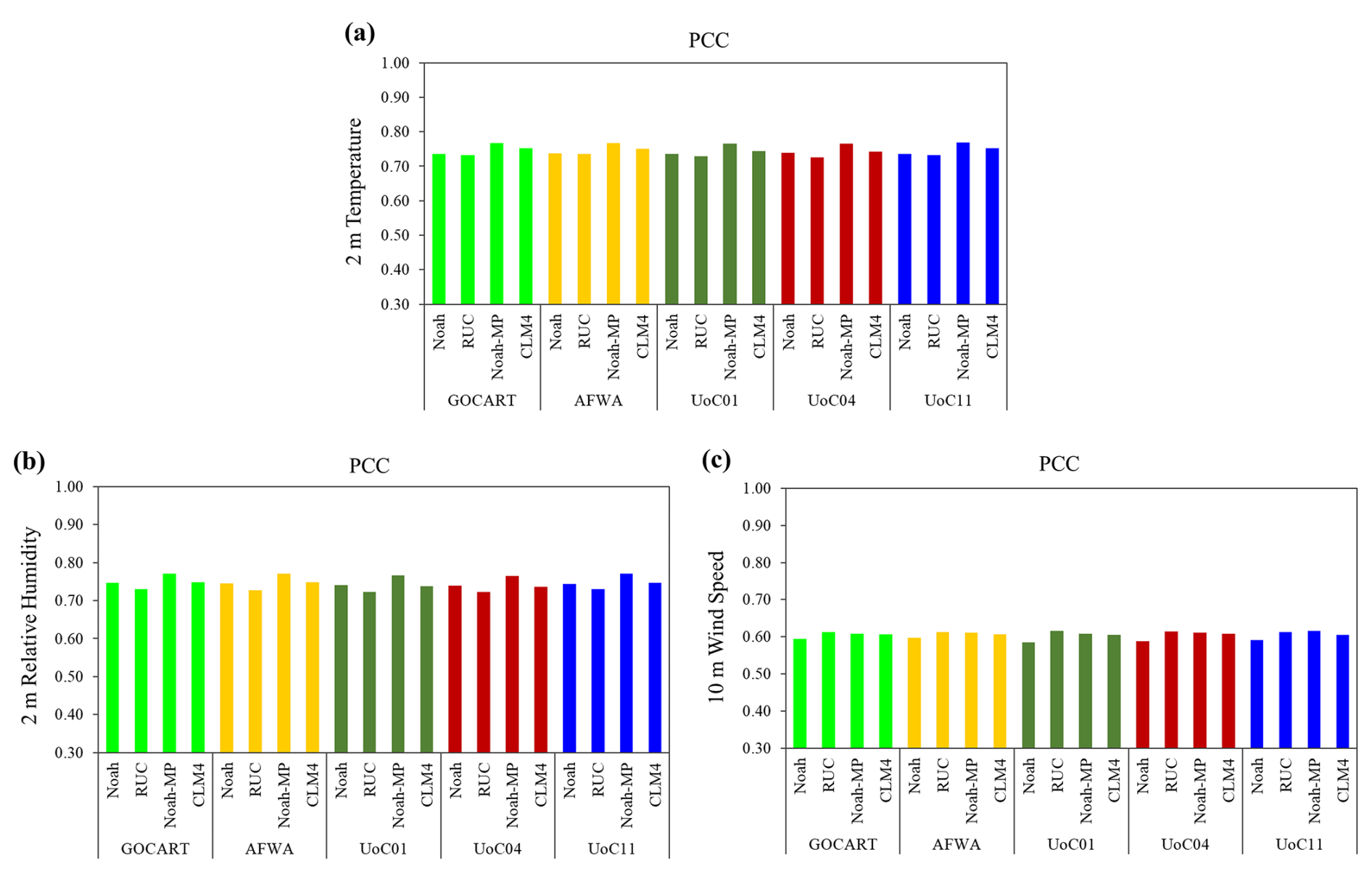
Figure 4 Pearson's correlation coefficient (PCC) of all scheme combinations for (a) T2m, (b) RH2m, and (c) WS10m, respectively, using the ASOS data. The y axis represents values greater than 0.3, indicating the minimum threshold for a moderate correlation. The values are averaged over the stations (see Fig. 3c).

Figure S1 shows the RMSE for all scheme combinations: (1) for T2m, Noah-MP-based combinations showed the best performance, followed by Noah-, CLM4-, and RUC-based combinations (Fig. S1a); (2) for RH2m, Noah-MP- and Noah-based combinations showed similarly good performance, followed by CLM4- and RUC-based combinations (Fig. S1b); and (3) for WS10m, Noah-MP-based combinations still showed the best performance, followed by RUC-based combinations (Fig. S1c). Figure S2 shows the MBE for all scheme combinations: (1) for T2m, Noah-MP- and Noah-based combinations showed similarly small MBEs, with a negative trend across all experiments (Fig. S2a); (2) for RH2m, Noah-MP- and Noah-based combinations also showed similarly good performance, with positive bias across all experiments (Fig. S2b); and (3) for WS10m, Noah-MP-based combination showed the best performance, with positive bias (Fig. S2c).

Overall, for surface meteorological variables, the Noah-MP-based combinations showed the best performance. The Noah-MP scheme provides reliable lower boundary conditions by accurately representing surface variables through more precise calculations of heat and moisture fluxes compared to other land surface schemes within the planetary boundary layer (Rizza et al., 2018; Wang et al., 2023).

Figure 5 shows the scatter plot of WS10m for UoC04-based combinations. In these combinations, the simulated values exhibited a clear tendency to overestimate compared to the observed values. Notably, UoC04-Noah-MP, which showed the best performance in WS10m validation based on MBE and RMSE, had the smallest intercept, indicating the lowest systematic bias among the four scheme combinations, followed by UoC04-RUC, UoC04-CLM4, and UoC04-Noah. Similar results were observed for T2m and RH2m (not shown). This finding aligns with the validation of meteorological variables, where Noah-MP-based combinations demonstrated the best performance.

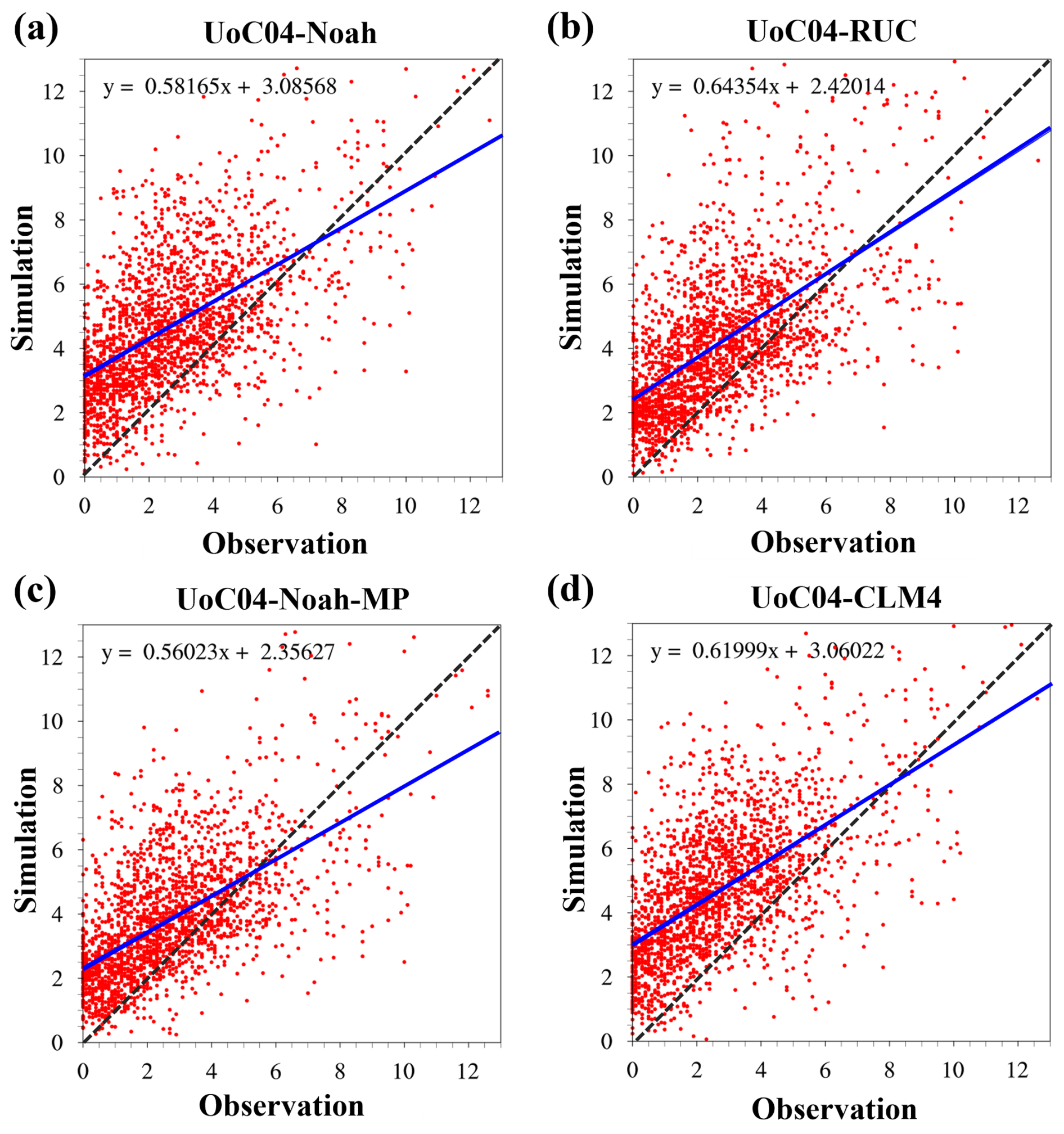
Figure 5 Scatter plots showing the relationship between observed and simulated values for WS10m, using UoC04-based combinations. Each panel represents a different scheme combination: (a) UoC04-Noah, (b) UoC04-RUC, (c) UoC04-Noah-MP, and (d) UoC04-CLM4. The dashed black line represents that the simulation perfectly matches the observation. The blue line indicates the linear regression fits the data, providing a relationship between the observed and simulated values.

Figure S3 shows time series comparisons of observations and CLM4-based combinations of T2m (Fig. S3a), RH2m (Fig. S3b), and WS10m (Fig. S3c) at two ASOS stations in South Korea – Yeongwol and Cheonan. The time series of T2m, RH2m, and WS10m showed very similar patterns, as meteorological variables are generally influenced more by land surface schemes than by dust emission schemes. For T2m, CLM4-based combinations showed an underestimation trend, whereas RH2m and WS10m tended to be overestimated. In particular, RH2m reached nearly 100 % before the ADS entered South Korea due to precipitation from a passing low-pressure system. The northwesterly winds behind this system, driven by an accompanying high-pressure system, often transport ADS from Inner Mongolia and the Gobi Desert to South Korea in spring (Lee et al., 2013). Meanwhile, despite the similar time series patterns of T2m, RH2m, and WS10m in the CLM4-based combinations, the PM₁₀ time series showed that GOCART-CLM4, AFWA-CLM4, and UoC11-CLM4 failed to reproduce the observed values (see Fig. 8). This failure is attributed to the inability to simulate dust emissions at the source regions, resulting in the absence of ADS transport to South Korea (see Figs. 12 and S9).

Figure S4 is the same as Fig. S3, except for UoC04-based combinations. T2m, RH2m, and WS10m showed significant differences based on the land surface schemes. Similar to the CLM4-based combinations, T2m was underestimated, whereas RH2m and WS10m were overestimated. For T2m, UoC04-Noah-MP closely matched the observations during the daytime, whereas UoC04-RUC performed better at night. For RH2m, UoC04-RUC, UoC04-Noah-MP, and UoC04-CLM4 matched the observations during periods of decreasing relative humidity, although UoC04-RUC showed noticeable differences. However, during periods of increasing RH2m, UoC04-based combinations differed significantly from the observations. For WS10m, UoC04-Noah and UoC04-CLM4 showed greater overestimation compared to UoC04-RUC and UoC04-Noah-MP.

3.1.2 Surface PM₁₀ concentrations

We compared the PM₁₀ prediction performance of all scheme combinations against in situ data from the Asian dust observation station (see the station locations in Fig. 3c). Figure 6 shows PCC, RMSE, and MBE for all scheme combinations. Overall, UoC04-CLM4 showed the best performance, followed by UoC01-CLM4. UoC04-RUC and UoC01-RUC also demonstrated relatively better performance compared to other scheme combinations. Conversely, the combinations of UoC01 and UoC04 with Noah and Noah-MP, as well as the combinations of GOCART, AFWA, and UoC11 with all land surface schemes, showed poor performance. The detailed descriptions of the verification results are as follows. (1) For PCC (Fig. 6a), UoC04-CLM4 showed the highest value (0.61), indicating a moderate correlation, followed by UoC01-CLM4 (0.60), UoC04-RUC (0.47), UoC01-RUC (0.44), UoC04-Noah-MP (0.35), and UoC01-Noah-MP (0.33), which also showed moderate correlations. Except for these schemes, the other combinations showed PCC values below 0.3, indicating a weak or almost no correlation. (2) For RMSE (Fig. 6b), UoC04-CLM4 showed the lowest value (199.59), indicating the best performance, followed by UoC01-CLM4 (201.618), UoC04-RUC (242.40), and UoC01-RUC (247.25). The other scheme combinations exhibited high values ranging 271–284, indicating relatively poor performance. (3) For MBE (Fig. 6c), all scheme combinations showed negative values, indicating an underestimation. UoC04-CLM4 showed the best performance (−6.29), followed by UoC01-CLM4 (−21.31), UoC04-RUC (−85.08), and UoC01-RUC (−90.28). In scheme combinations, excluding combinations of UoC04 and UoC01 with CLM4 and RUC, relatively more negative MBE (−137 to −120) was exhibited, indicating a significantly low performance compared to UoC04-CLM4.

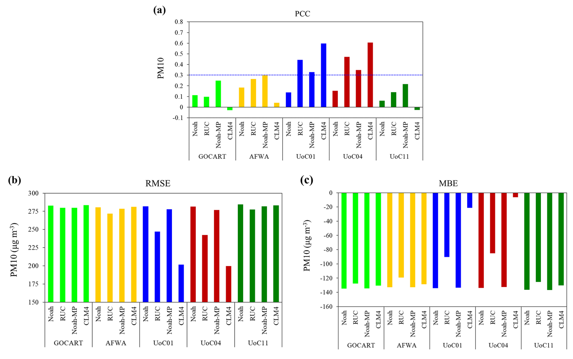
Figure 6 Verification results of all experiments for PM₁₀ concentrations; (a) PCC, (b) RMSE, and (c) MBE, respectively, using the in situ data. Based on PCC values, the dashed blue line represents the minimum threshold for a moderate correlation. The values are averaged over the stations (see Fig. 3c).

Figure 7 shows a scatter plot for CLM4-based combinations – the land surface scheme that showed the best prediction performance when combined with UoC04 and UoC01 in the verification (see Fig. 6). The x axis represents PM₁₀ observations, while the y axis indicates the simulated PM₁₀ values for each experiment. The red circles represent the simulated PM₁₀ values corresponding to the observations. In UoC04-CLM4 (Fig. 7c) and UoC01-CLM4 (Fig. 7d), the solid blue line shows that the trend between observed and simulated values generally increases positively compared to other scheme combinations. However, in UoC04-CLM4 – which showed the best performance in the verification – the model primarily overestimates values below approximately 180 µg m⁻³ and exhibits wider dispersion with underestimation tendencies for values above 180 µg m⁻³. In contrast, the other three combinations (Fig. 7a, b, and e) showed little to no correlation between observations and simulations, with a wider spread of data. Therefore, UoC04-CLM4 showed relatively better performance compared to the other scheme combinations.

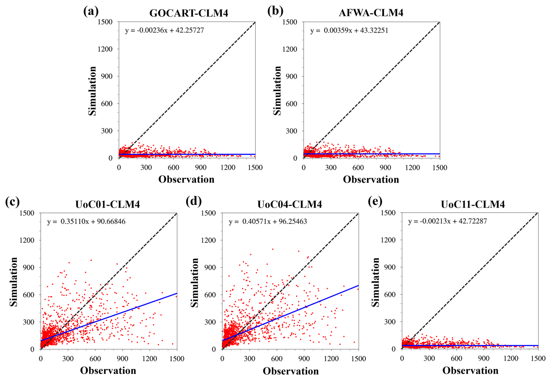
Figure 7 Same as in Fig. 5 but for PM₁₀ concentration, using CLM4-based combinations: (a) GOCART-CLM4, (b) AFWA-CLM4, (c) UoC01-CLM4, (d) UoC04-CLM4, and (e) UoC11-CLM4.

Figure S5 shows a scatter plot for the UoC04-based combinations – the dust emission scheme that showed the best prediction performance when combined with CLM4 in the verification (see Fig. 6). The UoC04-CLM4 combination showed the highest correlation between observed and simulated values among the UoC04-based combinations. In contrast, UoC04-Noah and UoC04-Noah-MP demonstrated little to no correlation, suggesting very low prediction reliability.

Table 4 shows the POD and FAR, calculated based on the PM₁₀ thresholds using the fine dust alert and ACWS in South Korea. A higher POD and a lower FAR indicate better prediction performance. Typically, a POD value below 0.5 indicates a failure to detect the observed events. The POD values for all scheme combinations at each threshold are as follows. (1) At 80 µg m⁻³, UoC04-CLM4 exhibited a very high POD (0.928), followed by UoC01-CLM4 (0.918), UoC04-RUC (0.544), and UoC01-RUC (0.516). The other experiments failed to predict the observed events, with POD ranging from 0.031 to 0.223. (2) At 150 µg m⁻³, UoC04-CLM4 also showed a high POD (0.799), followed by UoC01-CLM4 (0.758). Conversely, other experiments failed to detect the observed events or did not predict at all. (3) At 300 µg m⁻³, only UoC04-CLM4 achieved a POD of 0.520, surpassing the minimum detection threshold of 0.5. (4) At 800 µg m⁻³, UoC04-CLM4 failed to forecast the observed events, while the others did not predict at all. Overall, in terms of POD, UoC04-CLM4 showed the best prediction performance, with a POD of exceeding 0.5 up to 300 µg m⁻³.

Table 4 POD, FAR, and CSI values for each PM₁₀ threshold across all scheme combinations. The bold numbers indicate that POD is greater than 0.5 and CSI is relatively higher compared to the others. The dashes (–) indicate POD, FAR, and CSI values that cannot be calculated.

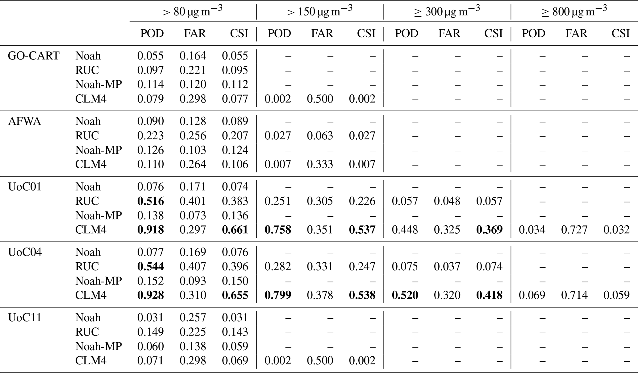
The FAR close to 0 indicates a low probability of false alarms. Note that FAR could lead to a decrease as the frequency of non-events increases because FAR considers non-events. The FAR values of all experiments for each threshold are as follows. (1) At 80 µg m⁻³, overall, Noah- and Noah-MP-based combinations showed relatively lower FAR than RUC- and CLM4-based combinations. (2) At 150 µg m⁻³, combinations of all dust emission schemes with RUC and CLM4 showed FARs ranging from 0.063 to 0.500. Notably, the AFWA-RUC showed the lowest FAR (0.063). Other combinations could not predict dust events – thus, calculating their FAR was impossible. (3) At 300 µg m⁻³, combinations of UoC01 and UoC04 with the RUC and CLM4 yielded FAR ranging from 0.048 to 0.325. Significantly, UoC04-RUC achieved the lowest FAR (0.037). As with the threshold of 151 µg m⁻³, other combinations were unable to simulate exceeding 300 µg m⁻³ of PM₁₀, making FAR calculations impossible. (4) At 800 µg m⁻³, FAR was calculated only for UoC04-CLM4 and UoC01-CLM4, showing high values exceeding 0.7.

When non-events occur frequently, FAR may falsely indicate skill improvement – highlighting the importance of considering both POD and FAR when evaluating prediction capability of detection. Therefore, considering both POD and FAR, UoC04-CLM4 demonstrated the best performance, followed by UoC01-CLM4.

In addition to POD and FAR, CSI provides a comprehensive evaluation of forecast accuracy by accounting for correct predictions, false alarms, and missed events. The CSI values for all scheme combinations for each threshold are as follows. (1) At 80 µg m⁻³, UoC04-CLM4 and UoC01-CLM4 exhibited the highest CSI values of 0.655 and 0.661, respectively, while the other schemes had significantly lower values, mostly below 0.2, except for UoC04-RUC (0.396) and UoC01-RUC (0.383). (2) At 150 µg m⁻³, UoC04-CLM4 and UoC01-CLM4 demonstrated CSI values of 0.538 and 0.537, respectively, indicating higher prediction accuracy compared to other scheme combinations. (3) At 300 µg m⁻³, UoC04-CLM4 outperformed the other schemes with a CSI of 0.418. Although this was a comparatively lower value, it still demonstrated better performance compared to the other schemes, most of which showed poor or non-existent forecast skill. (4) At 800 µg m⁻³, only UoC01-CLM4 and UoC04-CLM4 were calculated only for CSI, but both showed very low values of 0.059 and 0.032, respectively. Overall, UoC04-CLM4 consistently maintained CSI values above 0.5 up to 300 µg m⁻³, showing the highest performance among all experiments.

Figure 8 compares the PM₁₀ time series between observations and simulations, using combinations of all dust emission schemes and CLM4, at six Asian dust observation stations in South Korea – Seoul, Suwon, Yeongwol, Andong, Cheonan, and Mungyeong. UoC04-CLM4 and UoC01-CLM4 showed excellent performance in PM₁₀ prediction and effectively captured the onset and peak PM₁₀ concentrations when ADSs entered South Korea. During the analysis period, UoC04-CLM4 simulated slightly higher PM₁₀ concentrations than UoC01-CLM4 and approached the peak of PM₁₀ concentrations closer to observations. Conversely, GOCART-CLM4, AFWA-CLM4, and UoC11-CLM4 poorly simulated and significantly underestimated PM₁₀ concentrations throughout the forecast hours, leading to failure in predicting PM₁₀ concentrations during the mega ADS event in South Korea.

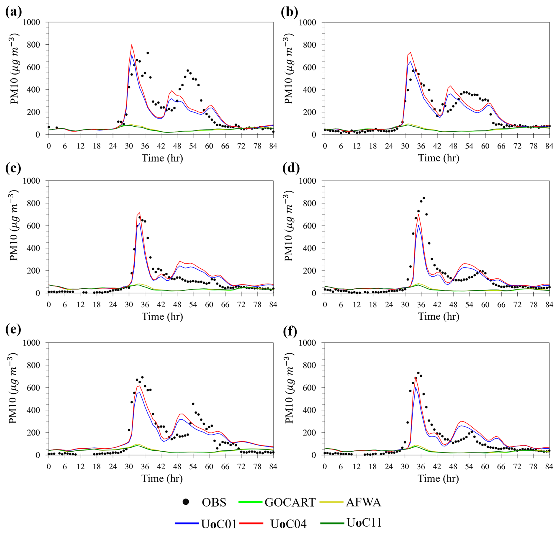
Figure 8 Time series comparison of PM₁₀ concentrations between observations and combinations of all dust emission schemes and CLM4 for (a) Seoul, (b) Suwon, (c) Yeongwol, (d) Andong, (e) Cheonan, and (f) Mungyeong. The black dots represent the observed PM₁₀ concentrations, while the colored lines depict various scheme combinations: lime green for GOCART-CLM4, yellow for AFWA-CLM4, blue for UoC01-CLM4, red for UoC04-CLM4, and green for UoC11-CLM4.

Figure S6 compares observations and forecasts of PM₁₀ concentrations for combinations of land surface schemes and UoC04. Note that PM₁₀ concentrations are substantially different for different land surface schemes. As noted in Fig. 8, UoC04-CLM4 simulated most similarly to observations, followed by UoC04-RUC. However, other scheme combinations, including UoC04-RUC, notably underestimated the PM₁₀ concentrations.

3.2 Evaluation using remote sensing and reanalysis data

3.2.1 Time series comparison of AOD: AERONET

Figure 9 shows the comparison of AOD time series between observations and simulations, using combinations of all dust emission schemes and CLM4, at six AERONET sites in South Korea: overall, UoC04-CLM4 and UoC01-CLM4 showed better agreement with observation than other experiments across all sites. On 29 March, a significant dust event, with AOD values exceeding 0.9, was observed at the Gwangju (Fig. 9c), Ulsan (Fig. 9e), and Gosan (Fig. 9f) sites. All experiments indicated underestimation, but GOCART-CLM4, AFWA-CLM4, and UoC11-CLM4 showed notably more significant underestimation than UoC04-CLM4 and UoC01-CLM4.

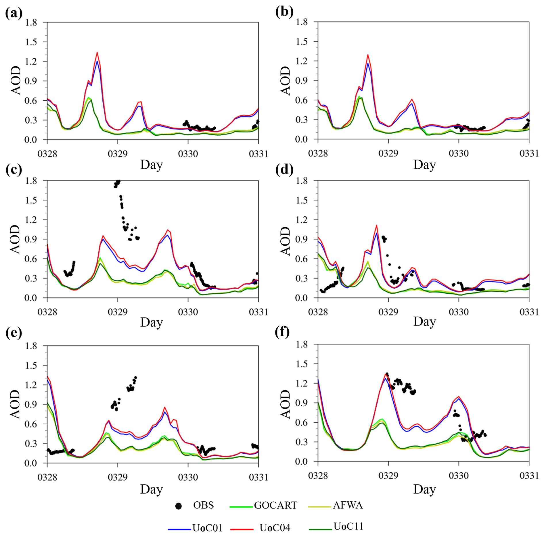
Figure 9 Time series of AERONET and simulated AOD in (a) Yonsei University, (b) Seoul, (c) Gwangju, (d) Gangneung, (e) Ulsan, and (f) Gosan in South Korea. The black dots represent AERONET AOD values, and the colored lines depict various scheme combinations – lime green for GOCART-CLM4, yellow for AFWA-CLM4, blue for UoC01-CLM4, red for UoC04-CLM4, and green for UoC11-CLM4.

Figure S7 shows the same as Fig. 9 except for combinations of all surface schemes and UoC04: overall, both UoC04-RUC and UoC04-CLM4 effectively captured the peak of ADSs around 29 March in South Korea – especially UoC04-RUC, which accurately simulated the AOD peak at the Ulsan site (Fig. S7e). However, UoC04-Noah and UoC04-Noah-MP significantly underestimated the peak, resulting in poorer AOD prediction performance.

3.2.2 Surface wind speed: MERRA-2

The near-surface wind across the source region is a critical factor for dust emission and transport. We identified areas with high values in the source region based on the MODIS AOD (see Fig. 12a) and validated WS10m from all experiments in this region against MERRA-2 data using MBE, RMSE, and PCC metrics. Figure 10 shows PCC, RMSE, and MBE for all scheme combinations. Consistent with the previous verification results for meteorological variables over South Korea, the scheme combinations with the same land surface scheme showed similar performance. The detailed verification results are as follows. (1) For PCC, all experiments exhibited high values ranging from 0.83 to 0.89. The PCC values of the scheme combinations using CLM4- and RUC-based combinations were relatively higher than those using Noah- and Noah-MP-based combinations (Fig. 10a). (2) For RMSE, UoC04-CLM4 (1.81) and UoC01-CLM4 (1.81) exhibited the same lowest values (Fig. 10b). These scheme combinations showed the best performance in PM₁₀ verification over South Korea. (3) For MBE, the scheme combinations based on Noah-MP showed positive MBE values, whereas the others exhibited negative MBE values. The CLM4-based combinations had the smallest magnitude of negative MBE values of around −0.02 (Fig. 10c). Overall, the CLM4-based combinations, including UoC04-CLM4 and UoC01-CLM4 – which demonstrated good performance in predicting PM₁₀ and AOD over South Korea – also showed the best performance for WS10m in the source region.

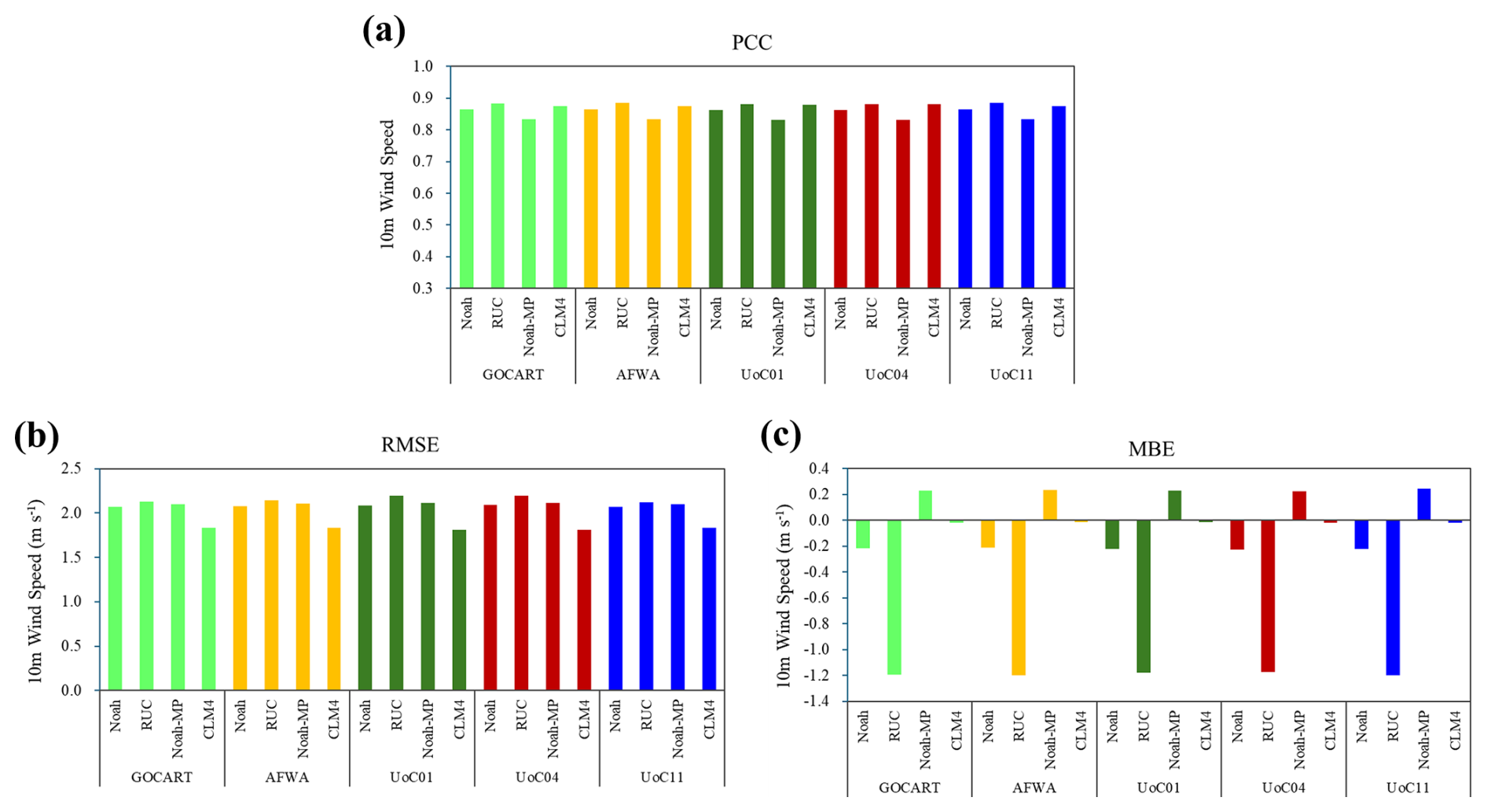
Figure 10 Verification results of all experiments for 10 m wind speed in the source region; (a) PCC, (b) RMSE, and (c) MBE, respectively, using MERRA-2. The values are averaged over grid points of MERRA-2 (see Fig. 3a).

Figure 11 shows the spatial evolution of surface total dust (DUST) concentrations and 10 m wind for CLM4-based combinations. Both MERRA-2 and the CLM4-based combinations similarly formed strong northwesterly winds in the source region, creating favorable conditions for dust emission and transport. However, MERRA-2, GOCART-CLM4, AFWA-CLM4, and UoC11-CLM4 exhibited significantly lower dust concentrations, whereas UoC04-CLM4 and UoC01-CLM4 showed notably higher concentrations (Fig. 11a). Subsequently, despite similar wind between MERRA-2 and CLM4-based combinations, only UoC04-CLM4 and UoC01-CLM4 successfully transported dust toward the Bohai Sea with strong northwesterly winds (Fig. 11b). As a result, UoC04-CLM4 and UoC01-CLM4 successfully transported dust to South Korea, reproducing a high-concentration dust event (Fig. 11c). These results are evident in comparison to MODIS AOD observations (see Fig. 12), as MERRA-2, GOCART-CLM4, AFWA-CLM4, and UoC11-CLM4 significantly underestimated dust concentrations, whereas UoC04-CLM4 and UoC01-CLM4 provided more reliable results.

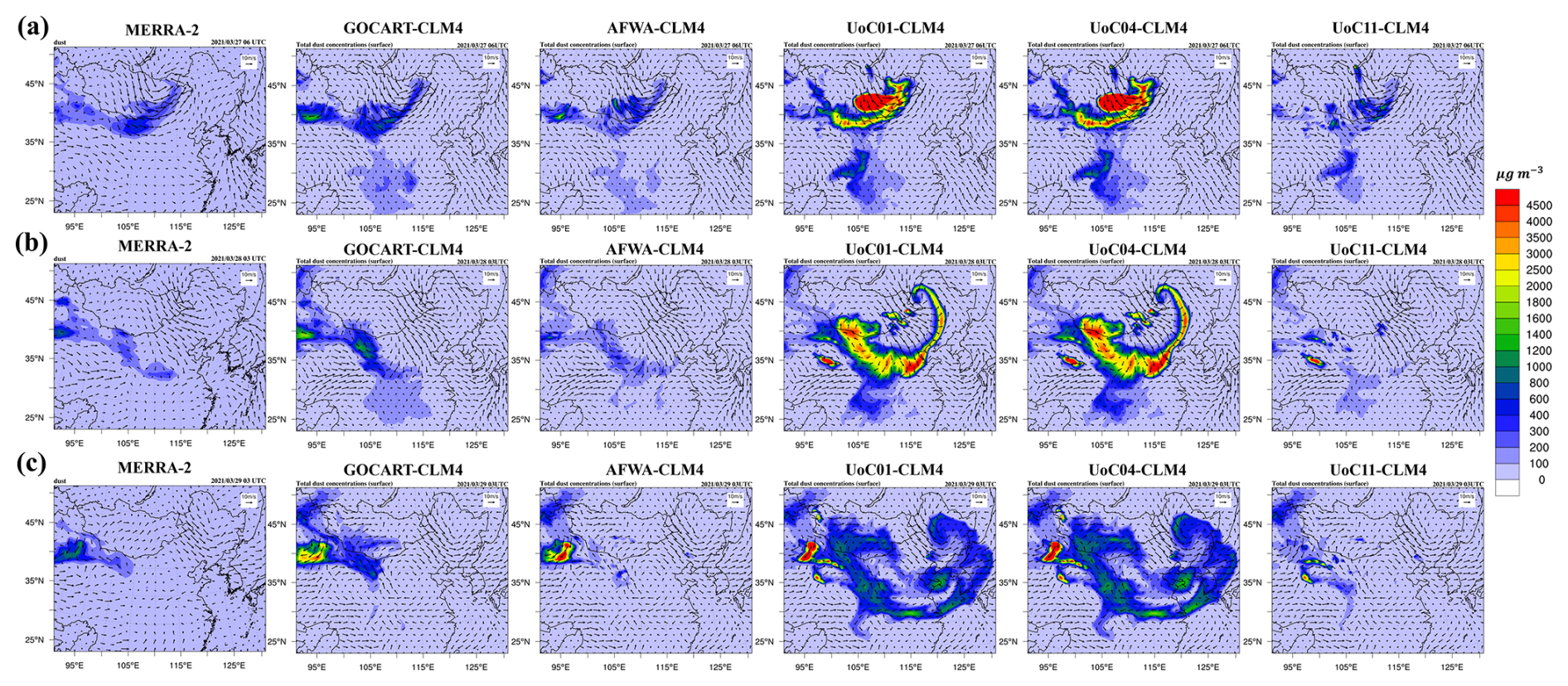
Figure 11 Spatial distribution of surface DUST concentrations (µg m⁻³) and 10 m wind (m s⁻¹) in the model domain for MERRA-2, and combinations of all dust emission schemes and CLM4: (a) dust emission in the Gobi/Inner Mongolia desert at 06:00 UTC on 27 March, (b) transport towards the Bohai Sea at 03:00 UTC on 28 March, and (c) appearance in South Korea at 03:00 UTC on 29 March 2021.

Figure S8 is the same as Fig. 11, except for the UoC04-based combinations. The wind patterns in the dust emission and transport processes were similar between MERRA-2 and the UoC04-based combinations in the source region (Fig. S8a and b). However, as dust was transported into South Korea, the wind over the Yellow Sea was weaker in MERRA-2 but stronger in the UoC04-based combinations (Fig. S8c). In terms of dust concentrations, UoC04-RUC and UoC04-CLM4 provided the most reliable simulations overall.

3.2.3 Spatial distribution of AOD: MODIS

Figure 12 shows the spatial distribution of AOD, comparing dust evolution processes – dust emission (Fig. 12a), transport (Fig. 12b), and appearance in South Korea (Fig. 12c) – among MODIS (i.e., observation), MERRA-2 (i.e., reanalysis), and combinations of dust emission schemes and CLM4 (i.e., model results). The comparison for each stage is as follows. (1) At 05:00 UTC on 27 March 2021 (Fig. 12a), dust emission stage, MODIS AOD notably exceeded 1.8 over the Gobi Desert/Inner Mongolia. UoC04-CLM4 and UoC01-CLM4 showed AOD values similar to MODIS with over 1.8. In contrast, MERRA-2, GOCART-CLM4, AFWA-CLM4, and UoC11-CLM4 showed significantly low values below 0.5, failing to simulate the dust origin. (2) At 03:00 UTC on 28 March 2021 (Fig. 12b), while maintaining high values (> 1.8), MODIS AOD moved towards the Bohai Bay, including the Shandong Peninsula and the Liaodong Peninsula. UoC04-CLM4 and UoC01-CLM4 showed a spatial distribution similar to MODIS AOD. However, MERRA-2 and the other scheme combinations did not simulate the dust transportation due to the absence of dust emission in the source region. (3) At 03:00 UTC on 29 March 2021 (Fig. 12c), as the dust flows into the inland of South Korea, the MODIS AOD exceeded 1.0 in the southern and southwestern regions of South Korea. MERRA-2, UoC04-CLM4, and UoC01-CLM4 underestimated AOD compared to MODIS, particularly in the southern and southwestern regions (≤ 0.6); the other scheme combinations failed in the AOD simulation (≤ 0.3). In summary, while UoC04-CLM4 and UoC01-CLM4 effectively simulated the spatial evolution processes of dust in South Korea similar to MODIS AOD, they showed a tendency to overestimate. Conversely, MERRA-2, GOCART-CLM4, AFWA-CLM4, and UoC11-CLM4 failed to predict AODs at all three processes, with a substantial underestimation.

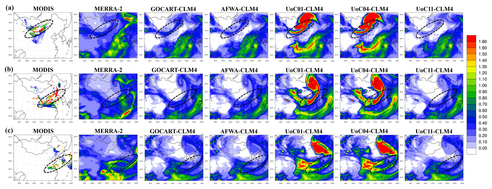
Figure 12 Spatial distribution of AOD in the model domain for MODIS, MERRA-2, and combinations of all dust emission schemes and CLM4: (a) dust emission in the Gobi/Inner Mongolia desert at 05:00 UTC on 27 March, (b) transport towards the Bohai Sea at 03:00 UTC on 28 March, and (c) appearance in South Korea at 02:00 UTC on 29 March 2021. The dashed black circles represent the main comparison regions of MODIS and each experiment.

Figure S9 shows the same as in Fig. 12 except for combinations of land surface schemes and UoC04. MERRA-2, UoC04-Noah, and UoC04-Noah-MP tended to underestimate and consequently failed to simulate the dust storm accurately. In contrast, UoC04-RUC and UoC04-CLM4 exhibited a strong tendency to overestimation. Nevertheless, from the origin of the source region to the appearance in South Korea, their simulations were closer to MODIS than those from other experiments.

3.2.4 Vertical distributions of extinction coefficients and dust concentrations: CALIPSO

Figure 13 shows a comparison of the vertical profiles of extinction coefficients between simulations (550 nm) – using CLM4-based combinations – and CALIPSO observations (532 nm). At 05:00 UTC on 28 March, the CALIPSO orbit passed through the Bohai Bay, including the Shandong Peninsula (see Fig. 3a), where high extinction coefficients were observed (117–120° E and 36–41° N) (Fig. 13a). Compared to the CALIPSO observations, overall, the extinction coefficients in UoC04-CLM4 and UoC01-CLM4 are consistent with the observations, particularly in regions with high values over the Bohai Bay and the Shandong Peninsula (Fig. 13d and e). In contrast, GOCART-CLM4, AFWA-CLM4, and UoC11-CLM4 significantly underestimate the values. This finding is consistent with the MODIS AOD (see Fig. 12b) and supports the reliability of the vertical distributions of DUST concentrations from the scheme combinations (see Fig. 14).

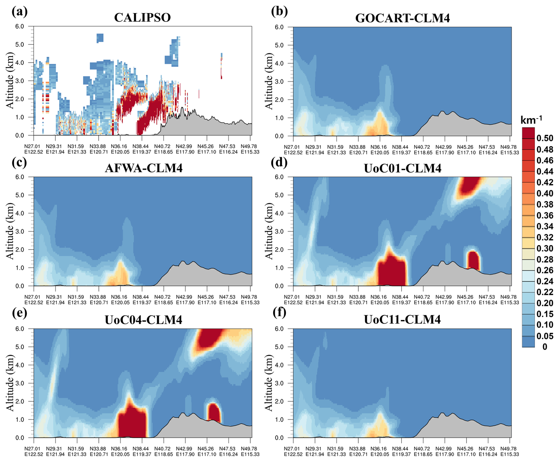
Figure 13 Vertical distributions of aerosol extinction coefficient for (a) CALIPSO, (b) GOCART-CLM4, (c) AFWA-CLM4, (d) UoC01-CLM4, (e) UoC04-CLM4, and (f) UoC11-CLM4 at 05:00 UTC on 28 March 2021. Dotted blue lines in Fig. 3a represent the sectional paths.

Figure S10 is the same as Fig. 13, except for the UoC04-based combinations. UoC04-CLM4 showed the greatest similarity to the observations (Fig. S10e), whereas UoC04-RUC simulated a too-narrow horizontal extent of high extinction coefficients (Fig. S10c). In contrast, UoC04-Noah and UoC04-Noah-MP significantly underestimate the values (Fig. S10b and d).

Figure 14 shows the vertical distributions of DUST concentrations along the main route of the ADS from the dust source regions to South Korea (see Fig. 3a), representing the DUST concentrations from all particle size bins in WRF-Chem. The comparisons of combinations of dust emission schemes and CLM4 are as follows. (1) At 12:00 UTC on 27 March 2021, GOCART-CLM4 and AFWA-CLM4 simulated dust concentrations very weakly (≤ 450 µg m⁻³) from the dust source region. In contrast, UoC04-CLM4 and UoC01-CLM4 showed dust concentrations surpassing 3000 µg m⁻³ up to 9.5 km over the dust source region, which is more than 6 times higher than those of GOCART-CLM4 and AFWA-CLM4. UoC11-CLM4 simulated DUST concentrations higher than GOCART-CLM4 and AFWA-CLM4 but lower than UoC04-CLM4 and UoC01-CLM4. During this period, westerly winds prevailed in the source region, while easterly winds persisted over the Bohai Sea and Yellow Sea. (2) At 02:00 UTC on 28 March, UoC04-CLM4 and UoC01-CLM4 indicated a shift from easterly winds to westerly winds over the Bohai and Yellow Sea, which initiated the movement of dust from the source region, with both having very similar patterns. Overall, the maximum altitude of dust has decreased, and DUST concentrations above 1000 µg m⁻³ were simulated up to approximately 6 km. Since other experiments simulated very low dust concentrations in the source region, almost no transport was observed. (3) At 12:00 UTC on 28 March, while westerly winds persisted in UoC04-CLM4 and UoC01-CLM4, DUST concentrations exceeding 1000 µg m⁻³ passed through the Yellow Sea at altitudes of approximately 4.5 km. (4) At 02:00 UTC on 29 March, both UoC04-CLM4 and UoC01-CLM4 simulated DUST concentrations exceeding 500 µg m⁻³ at the lowest altitude as the ADS reached South Korea.

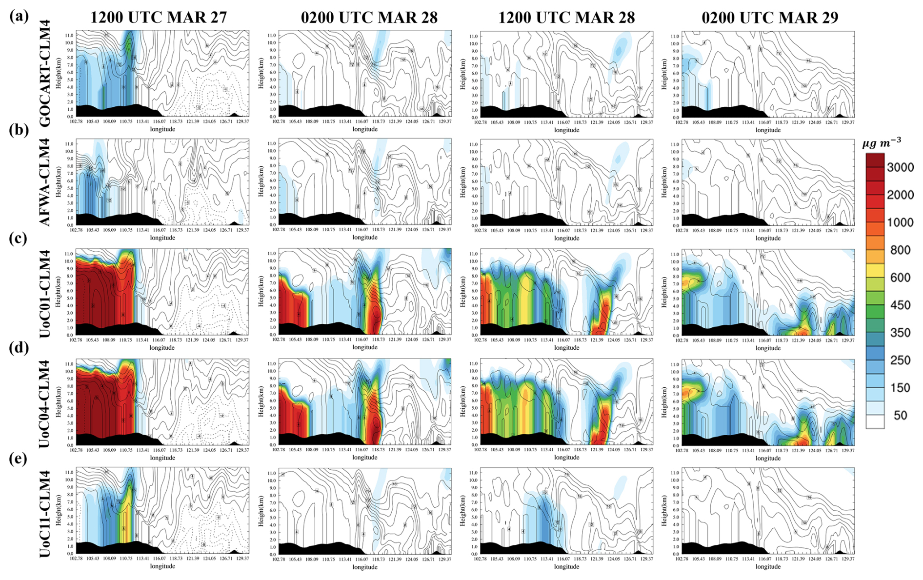
Figure 14 Vertical distributions of the DUST concentrations simulated by the combinations of all dust emission schemes and CLM4 for (a) GOCART-CLM4, (b) AFWA-CLM4, (c) UoC01-CLM4, (d) UoC04-CLM4, and (e) UoC11-CLM4, for given different times. The solid black lines and dashed black lines denote the westerly and easterly wind speeds, respectively. The colored shading represents the DUST concentration. The black shading indicates topographic height. The location of the cross section is referenced in Fig. 3a.

Figure S11 shows the same as Fig. 14 except for combinations of all land surface schemes and UoC04. (1) At 12:00 UTC on 27 March 2021, UoC04-RUC and UoC04-CLM4 simulated DUST concentrations above 3000 µg m⁻³ from the source region, with UoC04-RUC simulating dust to higher altitudes than UoC04-CLM4. In contrast, UoC04-Noah and UoC04-Noah-MP simulated significantly weaker DUST concentrations. (2) At 02:00 UTC on 28 March, UoC04-RUC and UoC04-CLM4 simulated dust transport towards the Bohai Sea by westerly winds. Once dust reached the Bohai Sea, UoC04-RUC showed primarily higher concentrations in the upper levels, while UoC04-CLM4 revealed higher concentrations at lower altitudes. UoC04-Noah and UoC04-Noah-MP did not simulate significant dust emissions from the source region, resulting in a lack of simulated dust transport. (3) At 12:00 UTC on 28 March, as the dust passed over the Yellow Sea, UoC04-RUC simulated DUST concentrations above 1500 µg m⁻³ up to approximately 9.5 km altitude. Meanwhile, UoC04-CLM4 simulated similar concentrations up to about 5 km, primarily at lower altitudes. (4) At 02:00 UTC on 29 March, as dust flowed into South Korea, UoC04-CLM4 simulated higher concentrations than UoC04-RUC, and dust was also simulated over the Yellow Sea. UoC04-Noah and UoC04-Noah-MP did not simulate any dust in South Korea.

3.3 Impact of scheme combinations on dust emission

The sensitivity experiments showed that each scheme combination produced different simulation results for meteorological variables and air quality variables over South Korea, with notable differences in PM₁₀, AOD, and DUST. To identify the underlying causes of these differences, we analyzed the meteorological conditions and surface DUST at the source regions for each scheme combination. The analysis focused on a specific point (44.18° N, 110.61° E) (see Fig. 3a) in the source regions where high MODIS AOD was observed during the dust emission period (see Fig. 12a). In general, in dust source regions, higher 2 m temperature, lower 2 m relative humidity, and stronger 10 m wind speed increase the probability of dust occurrence – high temperature and low humidity dry the surface, making it easier for dust particles to be lifted, and strong winds transport the dust into the atmosphere (Yang et al., 2019).

Figure S12 shows the time series of DUST, T2m, RH2m, and WS10m for UoC04-based combinations at the analysis point. The light orange shading indicates the period with the higher T2m, lower RH2m, stronger WS10m, and the initial increase in DUST. Overall, the meteorological variables varied depending on the scheme combination but were consistent with the general conditions required for dust emission. Notably, higher DUST concentrations were observed in UoC04-CLM4 and UoC01-CLM4, whereas lower concentrations were found in UoC04-Noah and UoC04-Noah-MP (Fig. S12a). These differences reflect the unique characteristics of each land surface scheme, despite using the same UoC04 parameterization.

In general, aeolian erosion, which contributes to dust emission in arid and semi-arid regions, occurs when the friction velocity is greater than the threshold value. Threshold values vary depending on soil properties and conditions, such as soil texture, particle size, and soil moisture (Fécan et al., 1999). The UoC schemes first calculate u_*t for dry and bare surface and then incorporate surface roughness features and soil moisture content to derive a more realistic threshold friction velocity (Shao and Lu, 2000). The calculation of u_*t is as follows:

$$\begin{array}{}\text{(13)}& u_{*t}=u_{*t}\left({\mathrm{dry}}_{\mathrm{bare}}\right)f_{\mathrm{r}}{f}_{\mathrm{s}},\end{array}$$

where u_*t(dry_bare) represents the threshold friction velocity for dry and bare surfaces, f_r indicates roughness features, and f_s denotes soil moisture content (Fécan et al., 1999). f_r is calculated based on the drag partition theory, whereas f_s is explicitly related to the land surface model. The latter is computed using the following equation:

$$\begin{array}{}\text{(14)}& f_{\mathrm{s}}=\sqrt{\mathrm{1}+a\left(i\right)(S-S_{\mathrm{dry}}(i){)}^{b\left(i\right)}},\end{array}$$

where i represents the soil texture index, which ranges from 1 to 12 (e.g., 1: sand; 2: loamy sand; 3: sandy loam; etc.); a(i), b(i), and S_dry(i) indicate tabulated parameter values corresponding to the soil texture index, respectively. Here, S represents soil moisture, and S_dry(i) denotes the dry soil moisture threshold at which direct evaporation from the topsoil layer ends. This threshold varies depending on the land surface schemes, influencing the explicit calculation of different u_*t values and ultimately playing a significant role in the dust emission process.

Figure 15 shows the time series of DUST, u_*t and u_*, for UoC04-based combinations. The light orange shading marks periods of simulated dust emission. The DUST concentrations showed significant differences depending on the land surface scheme. Details are as follows. (1) In the first shaded period, UoC04-CLM4 exhibited the highest DUST concentration, followed by UoC04-RUC, UoC04-Noah-MP, and UoC04-Noah. In the second, the DUST concentrations were lower than in the first, with UoC04-RUC exhibiting the highest concentration, followed by UoC04-CLM4. In contrast, UoC04-Noah-MP and UoC04-Noah showed DUST concentrations close to zero (Fig. 15a). (2) For UoC04-Noah, u_* barely exceeded u_*t in the first period, resulting in very low DUST concentrations, whereas in the second period, u_* did not exceed u_*t, leading to DUST concentrations close to zero (Fig. 15b). (3) For UoC04-RUC, u_* significantly exceeded u_*t in both the first and second shaded periods, resulting in high DUST concentrations (Fig. 15c). (4) For UoC04-Noah-MP, u_* exceeded u_*t in the first period but only slightly exceeded it during the second period, resulting in very low dust concentrations in the first period and nearly zero in the second (Fig. 15d). (5) For UoC04-CLM4, a pattern similar to UoC04-RUC was observed, with u_* greatly exceeding u_*t, leading to high DUST concentrations (Fig. 15e).

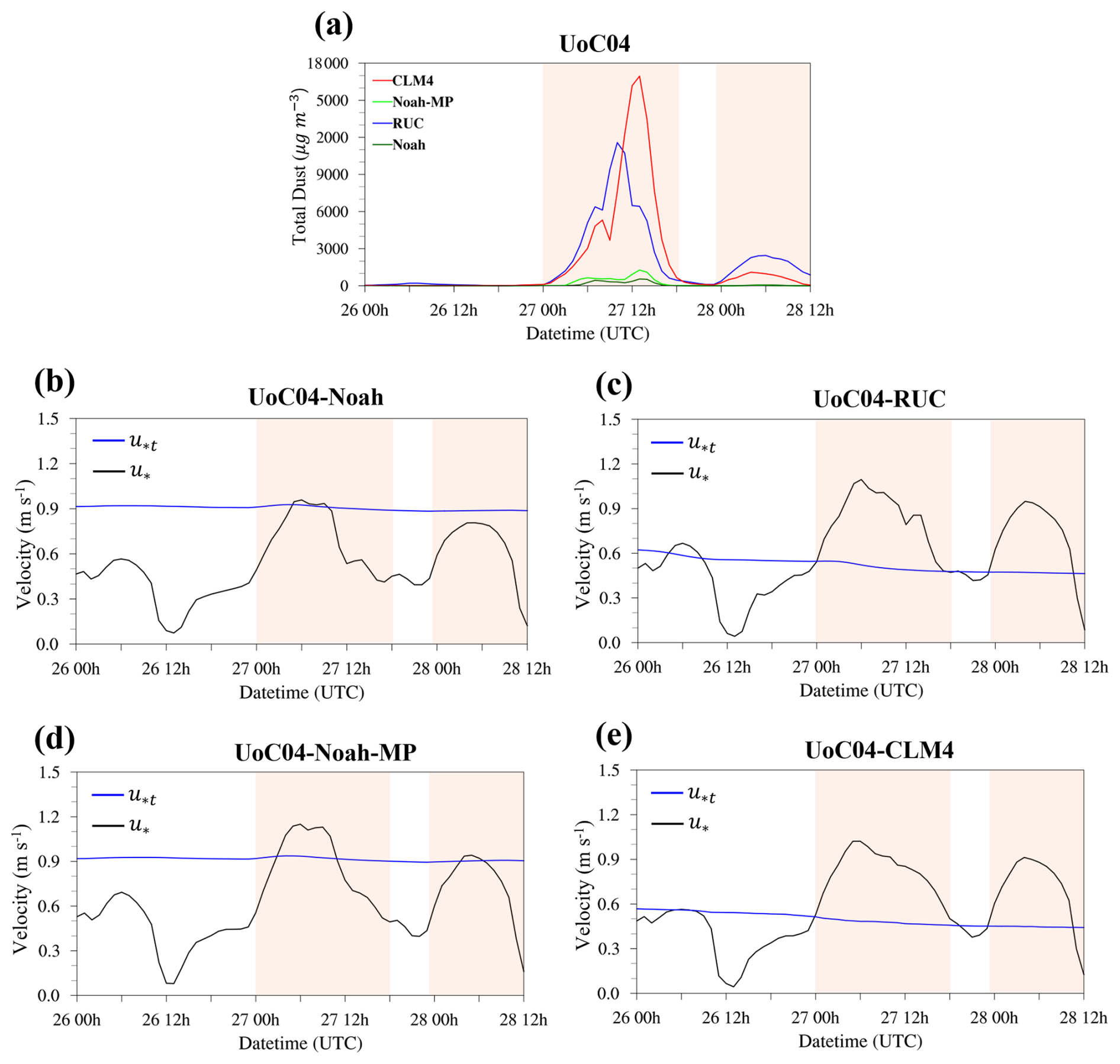
Figure 15 Hourly time series of surface DUST, threshold friction velocity (u_*t), and friction velocity (u_*) for combinations of all land surface schemes and UoC04. The light orange shadings indicate the periods of simulated dust emission: (a) surface DUST concentrations, u_*t, and u_* for (b) UoC04-Noah, (c) UoC04-RUC, (d) UoC04-Noah-MP, and (e) UoC04-CLM4.

In conclusion, UoC04-RUC and UoC04-CLM4 exhibited higher DUST concentrations despite u_* being similar to or even smaller than that of UoC04-Noah-MP. This results from the relatively lower u_*t in UoC04-RUC and UoC04-CLM4 compared to UoC04-Noah-MP, allowing u_* to exceed the threshold more easily. Additionally, the greater difference between u_*t and u_* contributed to the observed higher DUST concentrations. This highlights the interaction between dust emission schemes and land surface schemes, emphasizing the complexity of physical processes and surface–atmosphere interactions.

Figure S13 shows the time series of DUST, T2m, RH2m, and WS10m for CLM4-based combinations at the analysis point. UoC04-CLM4 showed the highest DUST concentrations, followed by UoC01-CLM4, while the other combinations exhibited significantly lower values. For T2m, RH2m, and WS10m, CLM4-based combinations showed similar patterns until their maximum or minimum values were reached. Afterward, UoC04-CLM4 and UoC01-CLM4, which simulated the highest DUST concentrations, exhibited distinct patterns compared to the other combinations – dust blocks or absorbs solar radiation, affecting temperature and humidity, thereby altering atmospheric thermal stability, which can influence the wind (Darvishi Boloorani et al., 2021). These differences reflect the unique characteristics of each dust emission scheme, despite using the same land surface model CLM4.

The GOCART-based schemes (GOCART and AFWA) and the UoC-based schemes (UoC01, UoC04, and UoC11) differ significantly in calculating dust emission flux. The GOCART-based schemes directly incorporate the dust erodibility factor into the calculation of dust emission flux, whereas the UoC-based schemes primarily use it as a dust source indicator. Additionally, the GOCART-based schemes use the porosity, whereas the UoC schemes account for various vegetation and soil physical properties – soil bulk density, vegetation fraction, disturbed particle size distribution, and soil plastic pressure – to enhance the accuracy of simulations (Zhao et al., 2020). Each scheme can be examined in detail as follows. (1) GOCART tends to overestimate u_t, leading to underpredictions of dust emissions, particularly for smaller particles (LeGrand et al., 2019). (2) AFWA, a modified version of GOCART, improves accuracy by replacing u_t with u_*t. It also incorporates soil clay content and aerodynamic roughness length, enabling more precise dust emission simulations. (3) UoC01 provides a more realistic representation of soil particle types by incorporating the size distribution of airborne dust particles, constrained by minimally disturbed p_m(d_i) and fully disturbed p_f(d_i) states (see Eq. 5). Naturally, dust particles generally exist as coatings on sand grains in sandy soils or as aggregates in clay-rich soils. In weak wind erosion, dust-coated sand particles and clay aggregates act as individual units and may not be released, representing a minimally disturbed state. In contrast, strong winds break them apart, increasing dust emissions in a fully disturbed state. (4) UoC04 is simplified compared to UoC01 but still considers p_m(d_i) and p_f(d_i). (5) UoC11 does not account for p_m(d_i) and p_f(d_i), thereby removing the kinematic impact on dust particle size distribution (Shao et al., 2011; see Eq. 8). This improves computational efficiency but reduces the accuracy of dust emission simulations. Consequently, as shown in Fig. S13a, the simulated DUST concentrations are low.

These differences in dust emission schemes led to distinct dust simulation results, even when the same land surface scheme was applied. In the CLM4-based combinations, UoC04 and UoC01 simulated high DUST concentrations in the source region (Fig. S13a), which were then transported to South Korea (Fig. 8). In contrast, GOCART, AFWA, and UoC11 failed to simulate both dust emissions and transport (Figs. S13a and 8). These findings are similar to those of Lee and Lee (2022), which emphasized the sensitivity of dust emission schemes to dust events in South Korea.

4 Conclusion

This study aims to evaluate the performance of various combinations of parameterization schemes – five for dust emission and four for land surface schemes – in the Weather Research and Forecasting Model coupled with Chemistry (WRF-Chem) for a mega Asian dust storm (ADS) event (i.e., 28–29 March 2021) over South Korea. Since the introduction of the ADS Crisis Warning System (ACWS) in South Korea in 2015, a nationwide caution stage was announced for the first time in 6 years on 29 March 2021. The PM₁₀ concentrations in Heuksando, located in the westernmost part of South Korea, were recorded as high as 1491 µg m⁻³ – one of the record-breaking events of severe Asian dust storms (ADSs) in South Korea. We evaluated the performance of various scheme combinations in WRF-Chem for this mega ADS event in the following steps.

First, we evaluated the performance of all scheme combinations in forecasting the surface meteorological variables related to dust storms – air temperature at 2 m (T2m), relative humidity at 2 m (RH2m), and wind speed at 10 m (WS10m) – and surface PM₁₀ concentrations. They were verified against surface observation data using various static metrics. (1) It turns out that the land surface schemes have a greater effect on surface meteorological variables than the dust emission schemes – showing little difference in model performance using different dust emission schemes. Notably, the combinations of all dust emission and Noah-MP schemes, known for their excellence as a land surface scheme, showed the best performance for meteorological variables. (2) For surface PM₁₀ concentrations, we observed significant variations of prediction performance across different scheme combinations, as the dust emission schemes directly influence the generation of dust storms. UoC04-CLM4 showed the best performance, followed by UoC01-CLM4, UoC04-RUC, and UoC01-RUC. In contrast, other scheme combinations showed very poor performance and failed to predict PM₁₀ in this study.

Second, we also compared the time series of simulated PM₁₀ and AOD with the in situ and remote sensing data. (1) For surface PM₁₀ concentrations, UoC04-CLM4 and UoC01-CLM4, which demonstrated good performance through verification, effectively captured the timing of dust inflow into South Korea and the peak PM₁₀ concentrations, with little difference between the two scheme combinations. However, the other experiments exhibited significant underestimations and completely failed to predict PM₁₀ concentrations. (2) For AOD, when strong dust storms occur and the AERONET AOD value is high, all experiments are underestimated, with combinations of RUC and CLM4 based on UoC01 and UoC04 showing the simulations most similar to the AERONET AOD.

Third, we found that UoC04-CLM4 and UoC01-CLM4 effectively simulated the three processes of emission, transport, and appearance in South Korea, similar to MODIS AOD, but with a tendency to overestimate these processes. In contrast, MERRA-2 and other scheme combinations failed to predict those processes, with significant underestimations.

Finally, we confirmed that UoC04-CLM4 and UoC01-CLM4 showed the highest consistency with CALIPSO observations in simulating extinction coefficients.

These findings highlight prominent differences in the capabilities among different scheme combinations, specifically dust emission and land surface schemes, in forecasting dust storms.

Since this study focuses on the selected parameterization schemes within the WRF-Chem model, it may just partially consider important factors that could affect the accuracy of ADS forecasting. Additionally, the evaluation is made for a specific mega ADS event, which may limit the generalization of the findings to other ADS events or regions. Nonetheless, this study provides valuable insights into the capabilities of various scheme combinations, thus laying a foundation for improvements in forecast skills for ADSs. Further research is needed to explore additional factors influencing dust storm forecasting accuracy and to generalize our findings to diverse weather conditions and regions.