Clustering simulated snow profiles to form avalanche forecast regions

This study presents a statistical clustering method that allows avalanche forecasters to explore patterns in simulated snow profiles. The method uses fuzzy analysis clustering to group small regions into larger forecast regions by considering snow profile characteristics, spatial arrangements, and temporal trends. We developed the method, tuned parameters, and present clustering results using operational snowpack model data and human hazard assessments from the Columbia Mountains of western Canada during the 2022–2023 and 2023–2024 seasons. The clustering results from simulated snow profiles closely matched actual forecast regions, effectively partitioning areas based on major patterns in avalanche hazard, such as varying danger ratings or avalanche problem types. By leveraging the uncertain predictions of fuzzy analysis clustering, this method can provide avalanche forecasters with a practical approach to interpreting complex snowpack model output and identifying regions of uncertainty. We provide practical and technical considerations to help integrate these methods into operational forecasting practices.

1 Introduction

Forecasting avalanche hazard over terrain is fundamental for effectively managing short-term snow avalanche risk (Canadian Avalanche Association, 2016). Forecasters assess the current hazard by interpreting weather, snowpack, and avalanche observations while also interpreting weather forecasts to predict future hazard conditions. In recent years, forecasters have shown interest in using numerical snowpack models to reduce their uncertainties (Morin et al., 2020). Models like SNOWPACK (Lehning et al., 1999) and Crocus (Brun et al., 1992) use meteorological data to provide predictions of snow stratigraphy and stability across spatial and temporal scales relevant to avalanche forecasting.

Several recent advancements have considerably enhanced the value of snowpack models for avalanche forecasting. First, improvements to numerical weather prediction models in complex terrain (Lundquist et al., 2020) allow snowpack simulations to be run in remote regions (Horton and Haegeli, 2022). Second, new post-processing models establish stronger connections with snow stability (Mayer et al., 2022) and avalanche hazard (Pérez-Guillén et al., 2022). Lastly, applying visual design principles (Horton et al., 2020) and snow profile processing tools (Herla et al., 2021, 2022) can enhance the communication of this information to forecasters. While operational model systems are beginning to incorporate these developments, their adoption into forecasting workflows remains gradual. Therefore, we need to present model output in simple, informative ways.

Statistical clustering methods provide an effective means of identifying and summarizing patterns within complex datasets. Bouchayer (2017) was the first to cluster simulated snow profiles by grouping profiles based on the specific surface areas of snow layers. Using a dynamic time-warping alignment method developed by Hagenmuller and Pilloix (2016), they constructed a hierarchical clustering tree by comparing vertical sequences of specific surface areas. Herla et al. (2021) expanded on this approach by incorporating generic categorical and numerical snowpack properties such as hand hardness and grain type into the dynamic time-warping process. This enabled them to employ hierarchical clustering methods to group snow profiles based on characteristics relevant to avalanche hazard assessment. Reuter et al. (2023) applied k-means clustering to simulated snow profiles by predicting avalanche problem types from the profiles and then clustering problem prevalence to explore the snow climatologies in the French Alps. While these clustering methods revealed patterns in simulated snowpack properties, they did not fully capture the spatial and temporal patterns important to avalanche forecasters.

To provide avalanche forecasters with more accessible and relevant snowpack model information, this paper presents a method for clustering simulated snow profiles into avalanche forecast regions. Our method expands upon the approach introduced by Herla et al. (2021), which partitions snow profiles based on avalanche hazard characteristics, by further addressing the operational requirements for coherent spatial and temporal patterns. We developed the method using operational snowpack simulations and human avalanche hazard assessments from the Columbia Mountains of western Canada. Section 2 describes the study area and data, and then Sect. 3 introduces the clustering method. After selecting appropriate parameters with data from the 2022–2023 season (Sect. 4), we present examples of the clustering results and compare them with human-assessed forecasts for both the 2022–2023 and 2023–2024 seasons in Sect. 5. To help others apply these methods, we discuss the practical and technical implications in Sect. 6.

2 Study area and data

2.1 Study area

We developed the clustering method using simulated snow profiles and human-assessed avalanche forecasts in the Columbia Mountains of western Canada (Fig. 1a). The Columbia Mountains have a transitional snow climate prone to storm slab and persistent slab avalanche problems (Shandro and Haegeli, 2018). Variations in weather and snowpack across the range often lead to distinct patterns in avalanche hazard, making it well-suited for exploring spatial clustering methods. For example, storm tracks can impact the northern and southern parts of the range differently, while orographic enhancement often results in heavier precipitation on the western sides of each subrange.

Public avalanche forecasters at Avalanche Canada, Canada's public avalanche warning service, divided the Columbia Mountains into 32 permanent subregion polygons for the 2022–2023 season (total area of 111 801 km²). The subregion polygons were revised for the 2023–2024 season by splitting 1 subregion into 2, increasing the total to 33, and making a few minor boundary adjustments. Forecasters aggregate these subregions into larger forecast regions daily based on their assessment of avalanche hazard conditions. In this study, subregions refer to the individual subregion polygons and regions refer to the aggregated groups of subregions, whether done by human forecasters or clustering methods.

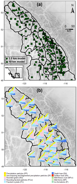
Figure 1 The study area and simulated snow profiles for the 2022–2023 season include (a) the Columbia Mountains, divided into 32 permanent subregions, with original snow profile locations based on grid points from two numerical weather prediction models (2.5 and 10 km resolutions); and (b) snow profile time series averaged within each subregion.

2.2 Simulated snow profiles

We obtained simulated snow profiles for the 2022–2023 and 2023–2024 seasons from Avalanche Canada's operational snowpack modelling system (Horton et al., 2023). This model system runs the SNOWPACK model (Lehning et al., 1999) with meteorological data from two numerical weather prediction models, the 2.5 km High Resolution Deterministic Prediction System and the 10 km Regional Deterministic Prediction System (Fig. 1a). The model generates daily profiles at 168 treeline elevation locations across the Columbia Mountains, each representing conditions in flat, sheltered terrain. Since this paper focuses on presenting a clustering method that applies to any spatially distributed snowpack simulation, the specific techniques used for generating these profiles are described in Appendix A.

To represent typical treeline elevation conditions in each subregion, we computed representative profiles using the dynamic time-warping barycenter-averaging method developed by Herla et al. (2022). This method aligns profile layers using dynamic time-warping, computes the prevalent grain type mode for each layer, and then averages the layer properties of each dominant mode (e.g., thickness, hardness, and temperature). Averaging was done for each day of the season at 16:00 PST to produce snow profile time series representing typical treeline conditions in each subregion (Fig. 1b). While these generalized profiles represent conditions in flat, sheltered treeline terrain at the scale of Avalanche Canada subregions, they do not capture the full range of conditions that avalanche forecasters consider when assessing conditions, such as those specific to certain elevations or aspects. However, the generalized profiles do a good job of capturing widespread new snow and persistent weak layers, which are key drivers of avalanche hazard in the Columbia Mountains.

2.3 Human-assessed forecast regions

Avalanche Canada issues daily public avalanche forecasts for the Columbia Mountains. Forecasters group subregions into semi-homogenous regions and assign danger ratings and avalanche problems to three elevation bands for each region. Our study periods started when daily forecasting began in the early winter and ended when forecasts switched to a single large region for spring conditions (11 November 2022 to 23 April 2023 and 1 December 2023 to 25 April 2024). System outages caused the operational snowpack model data to be unavailable on several days each season, leaving 115 and 98 d, when a complete set of model and human data was available for analysis in each season.

3 Clustering method

3.1 Distance between subregions

Many clustering methods use a distance matrix to quantify differences among data points (Kaufman and Rousseeuw, 2009). A distance metric measures the distance between each pair of points: identical points have a distance of 0, while dissimilar points have larger values. Pairwise distances are arranged in a matrix with rows and columns representing each data point. Our clustering method derives a metric to quantify the distance between subregions in a way that encourages similar subregions to be grouped (Fig. 2). Our distance metric “dist” considers three relevant criteria:

1. Snow profile characteristics. The snow profile distance dist_pro quantifies the similarity of snow profiles so that clustering will produce forecast regions with similar avalanche hazard characteristics.

2. Spatial arrangement. The spatial distance dist_geo quantifies the spatial arrangement of subregion polygons so that clustering will produce spatially contiguous regions.

3. Temporal stability. The sequential distance dist_seq quantifies the previous day's clustering results so that clustering will only change regions when there are substantial changes in snow profile characteristics.

After calculating these individual distance metrics, we compute the overall distance between subregions (dist) using a weighted mean:

$$\begin{array}{}\text{(1)}& \mathit{d}\mathit{i}\mathit{s}\mathit{t}=\left(\mathit{\alpha }\right)\mathit{d}\mathit{i}\mathit{s}{\mathit{t}}_{\mathrm{geo}}+\left(\mathit{\beta }\right)\mathit{d}\mathit{i}\mathit{s}{\mathit{t}}_{\mathrm{seq}}+(\mathrm{1}-\mathit{\alpha }-\mathit{\beta })\mathit{d}\mathit{i}\mathit{s}{\mathit{t}}_{\mathrm{pro}},\end{array}$$

where α is a weight controlling the relative significance of the spatial distance and β is a weight controlling the relative significance of the sequential distance.

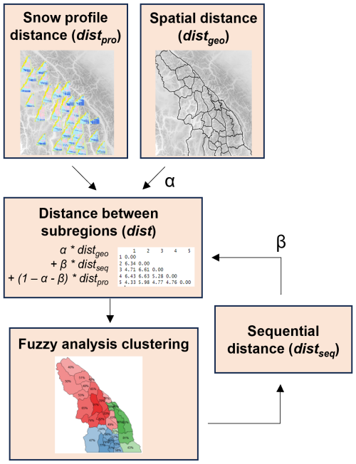
Figure 2 The clustering method derives an overall distance matrix integrating three key criteria: snow profile distance, spatial distance, and sequential distance. Snow profile distance is based on snow profile characteristics in simulated snow profiles, spatial distance is based on the arrangement of polygons, and sequential distance is based on the previous day's forecast regions.

3.1.1 Snow profile characteristics

We quantify the snow profile distance (dist_pro) with the snow profile similarity measure introduced by Herla et al. (2021). This method aligns two profiles onto a common height grid using dynamic time-warping and then compares the properties of the layers to assign a similarity score ranging from 0 to 1. The similarity scores are calculated using the sarp.snowprofile.alignment package for R (Herla et al., 2021, 2022), which offers various approaches to calculate the similarity of aligned profiles. These approaches weigh different combinations of grain type, grain size, layer hardness, and instability. To emphasize layer instability, we use an approach that computes a weighted sum of grain type similarity (37.5 %), hand hardness similarity (12.5 %), and layer instability similarity (50 %). Layer instability is determined with the random forest method developed by Mayer et al. (2022) to predict the probability of instability for each layer in a profile. Among the available similarity approaches in sarp.snowprofile.alignment, this one most closely aligns with avalanche forecasting by incorporating both mechanical properties (i.e., instability) and structural properties (i.e., grain type and hardness). Methods that focus purely on structural properties can overemphasize the importance of thick cohesive layers, but this approach weights thin unstable layers more heavily. We calculate the pairwise similarity of profiles each day and then subtract them from 1 to produce snow profile distance values.

3.1.2 Spatial arrangement

We consider the spatial distance between subregions to encourage geographically contiguous forecast regions. We designed the spatial distance (dist_geo) to reduce the distance between subregions in close geographic proximity while increasing the distance for spatially separated subregions. We derived the spatial distance matrix using a binary neighbourhood-based approach, where polygons sharing borders have a distance of 0 and polygons without shared borders have a distance of 1 (Chavent et al., 2018). The neighbourhood approach encourages spatially connected forecast regions, often forming elongated shapes that follow snow climates along mountain ranges. In contrast, tests using Euclidean distances produced forecast regions that were geographically close but more likely to span multiple snow climates.

3.1.3 Temporal stability

When clustering on consecutive days, the arrangement of forecast regions should vary in response to changing avalanche hazard conditions. However, clustering can be overly sensitive to subtle changes in the dataset, which can lead to excessive changes in regional boundaries that may not be practical for forecasting applications. To address this issue, we use a sequential distance (dist_seq) to incorporate some weight from the previous day's clustering results in a way that encourages subregions to remain in the same groups. Section 4.4 explains this approach in detail.

3.2 Fuzzy analysis clustering

Given the complexities of avalanche hazard assessment and snow profile simulations, we chose a fuzzy clustering method to explicitly highlight the uncertainties associated with assigning data points to clusters. Fuzzy clustering methods produce membership probabilities that allow data points to belong to multiple clusters simultaneously (Kaufman and Rousseeuw, 2009).

Our method uses a fuzzy variant of k-medoid clustering called fuzzy analysis clustering, or fanny. The fanny method, implemented in the cluster package for R and described by Kaufman and Rousseeuw (2009), assigns each data point i membership values u_iv between 0 and 1, quantifying its degree of belonging to cluster v. The method aims to minimize the objective function:

$$\begin{array}{}\text{(2)}& \sum _{v=\mathrm{1}}^k{\displaystyle \frac{{\sum }_{i=\mathrm{1}}^n{\sum }_{j=\mathrm{1}}^n\left(u_{iv}{)}^r\right(u_{jv}{)}^r\text{dist}(i,j)}{\mathrm{2}{\sum }_{j=\mathrm{1}}^n(u_{jv}{)}^r}},\end{array}$$

where n is the number of data points, k is the number of clusters, dist(i,j) is the distance between data points i and j, and r is the fuzziness parameter. The fuzziness parameter r, whose value can range between 1 and infinity, controls the degree of fuzziness in the clusters. As r approaches 1, clusters become increasingly crisp (i.e., k-medoid clustering), while higher values lead to complete fuzziness (i.e., data points have equal membership in every cluster). The method iteratively updates cluster centers using the medoid data point and recalculates membership values until the objective function in Eq. (2) converges (i.e., changes less than 10⁻¹⁵ between iterations).

We arrange the distances between subregions (dist) into a matrix and input them into the fanny method to derive cluster membership values for each subregion. This process requires specification of appropriate values for the fuzziness parameter r and the number of clusters k, as explained in Sect. 4.

4 Optimizing clustering parameters

To apply our clustering method, four parameters must be defined, i.e., α and β, which specify how much weight is given to the spatial and sequential distances (Eq. 1); the fuzziness parameter r, which determines the crispness of the cluster memberships; and the number of clusters to be estimated k (Eq. 2). Optimal values for these parameters will vary between contexts, so this section outlines methods for appropriate parameter selection.

We used grid searches (Feurer and Hutter, 2019) to systematically explore various parameter combinations with data from the 2022–2023 season, and then we used two approaches to select optimal values from the grid search: a cluster validation metric and a comparison with human-assessed forecast regions. We conducted two grid searches. The first grid search systematically explored combinations of $\mathit{\alpha }=\mathit{\{}\mathrm{0},\mathrm{0.05},\mathrm{0.1},\mathrm{\dots },\mathrm{0.5}\mathit{\}}$, $r=\mathit{\{}\mathrm{1.05},\mathrm{1.10},\mathrm{\dots },\mathrm{2}\mathit{\}}$, and $k=\mathit{\{}\mathrm{2},\mathrm{\dots },\mathrm{15}\mathit{\}}$, with each day treated as independent (i.e., β=0). Optimal values from this initial grid search informed a second grid search where sequential clustering was done over the 2023–2023 season with $\mathit{\beta }=\mathit{\{}\mathrm{0},\mathrm{0.01},\mathrm{\dots },\mathrm{0.25}\mathit{\}}$. The rationale for these ranges is explained in the following sections.

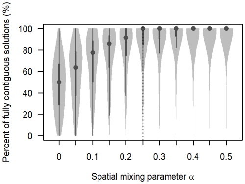
Figure 3 The percentage of grid search results that produced fully spatially contiguous regions when changing the spatial weight α. The violin plot shows the data distribution with a dot for the median, thick bars for the interquartile range, thin lines for the full range, and light-grey areas for higher data density. The optimal value chosen for this study was 0.25 (vertical dashed line).

4.1 Spatial weight

We examined the spatial arrangement of clusters resulting from the grid search to find the proportion of spatially contiguous to non-contiguous regions. The grid search covered $\mathit{\alpha }=\mathit{\{}\mathrm{0},\mathrm{0.05},\mathrm{0.1},\mathrm{\dots },\mathrm{0.5}\mathit{\}}$, ranging from scenarios where the distance was based solely on snow profile characteristics to those where snow profile and spatial distances were equally weighted. When considering only snow profile characteristics (i.e., α=0), 47 % of grid search solutions contained fully contiguous regions across all combinations of r and k (Fig. 3). The percentage of solutions with fully contiguous regions increased with higher values of α, reaching 96 % for α=0.5.

The optimal level of spatial contiguity depends on user preferences and the number and arrangement of subregions. While some non-contiguous regions may offer insights into similar snowpack patterns across large distances, an excessive number can result in incoherent spatial patterns. In this study, we selected α=0.25 to maximize the weight on snow profile characteristics while constraining the majority of the solutions to produce fully contiguous regions.

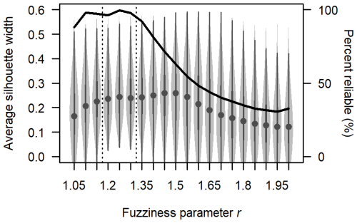
Figure 4 The impact of varying the fuzziness parameter r on fuzzy analysis clustering results. The violin plots show the distribution of the average silhouette width for grid search results with different values of r, with dots for the median, thick bars for the interquartile range, thin lines for the full range, and light-grey areas for higher data density. The percentage of reliable results that converged to the correct number of clusters without complete fuzziness is shown with the black line. The optimal range of r values for this study was 1.2 to 1.3 (between the vertical dashed lines).

4.2 Fuzziness parameter

The fuzziness parameter r plays a crucial role in balancing the crispness and fuzziness of clusters, ensuring they are neither overly sharp (all membership values are 0 or 1) nor completely fuzzy (all membership values are $\mathrm{1}/k$). The grid search covered $r=\mathit{\{}\mathrm{1.05},\mathrm{1.1},\mathrm{\dots },\mathrm{2}\mathit{\}}$, ranging from just above the minimum value of 1 to the default value of 2. We did not extend our grid search beyond r=2 because higher values consistently resulted in complete fuzziness for our dataset. The fanny algorithm in R warns of poorly fitted clusters when the solution does not converge (r is too small) or when the memberships are completely fuzzy (r is too large), either of which can cause the algorithm to partition the data into fewer than k clusters. We flagged grid search results without these issues as reliable.

We used the average silhouette width (ASW) to assess the quality of each reliable clustering result. This metric compares the average distance of each data point to others within the same cluster with the average distance to points in other clusters (Kaufman and Rousseeuw, 2009). An ASW close to 1 indicates that data points are well-matched to their own clusters and poorly matched to other clusters, values near 0 suggest that data points are on the boundary between clusters, and negative values imply that data points may be misclassified, as they are closer to points in other clusters than to those within their own.

The grid search produced reliable solutions in over 95 % of cases when $\mathrm{1.1}\le r\le \mathrm{1.3}$, with 99.5 % reliability at r=1.25 (Fig. 4). The highest ASW occurred when $\mathrm{1.2}\le r\le \mathrm{1.5}$, with median values above 0.25. Only the $\mathrm{1.2}\le r\le \mathrm{1.3}$ range avoided negative ASWs, suggesting this range is optimal for producing reliable results that balance crispness and fuzziness in our dataset. Our clustering implementation computed solutions for $r=\mathit{\{}\mathrm{1.2},\mathrm{1.225},\mathrm{1.25},\mathrm{1.275},\mathrm{1.3}\mathit{\}}$ and then selected the reliable solution with the largest ASW.

4.3 Number of clusters

The grid search spanned $k=\mathit{\{}\mathrm{2},\mathrm{\dots },\mathrm{15}\mathit{\}}$, with 15 being the maximum possible k for fuzzy analysis clustering of our n=32 regions. We considered two approaches for selecting the optimal k: (1) maximizing the ASW or (2) aligning the cluster resolution with the resolution of human-assessed regions.

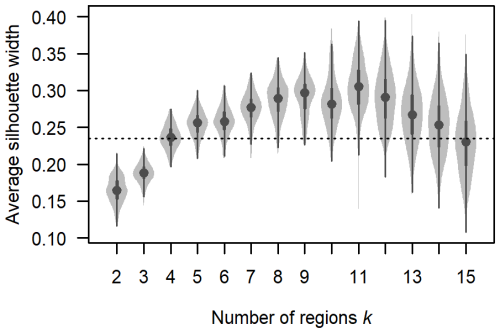
Figure 5 Average silhouette width (ASW) for different numbers of regions $k=\mathit{\{}\mathrm{2},\mathrm{\dots },\mathrm{15}\mathit{\}}$ over grid search results with a spatial weight (α=0.25) and a fuzziness parameter ($\mathrm{1.2}\le r\le \mathrm{1.3}$). The violin plot shows the distribution of the ASW with a dot for the median, thick bars for the interquartile range, thin lines for the full range, and light-grey areas for higher data density. The horizontal dashed line shows the threshold ASW used to select a similar number of clusters to human-assessed regions (0.23).

Figure 5 shows the ASWs from the grid search using the optimal spatial weight (α=0.25) and fuzziness parameter range ($\mathrm{1.2}\le r\le \mathrm{1.3}$). Removing the results with suboptimal values of α and r better highlights the typical trends in ASW as k changes. The ASW typically reached peak values for k values between 8 and 12, with median values greater than 0.28. However, plotting ASW on individual days found relatively flat peaks (not shown), indicating that selecting the number of clusters from the maximum ASW could result in arbitrary and fluctuating regions over time.

A better strategy for selecting the optimal number of regions was to choose the smallest k where the ASW exceeded a threshold, ensuring smaller and more consistent k values over time. We set the threshold by comparing grid search cases where k matched the number of human-assessed regions each day and where k was one fewer. A two-sample t test found that a threshold ASW of 0.23 best separated these groups. Our clustering implementation used this threshold to select the optimal number of clusters each day.

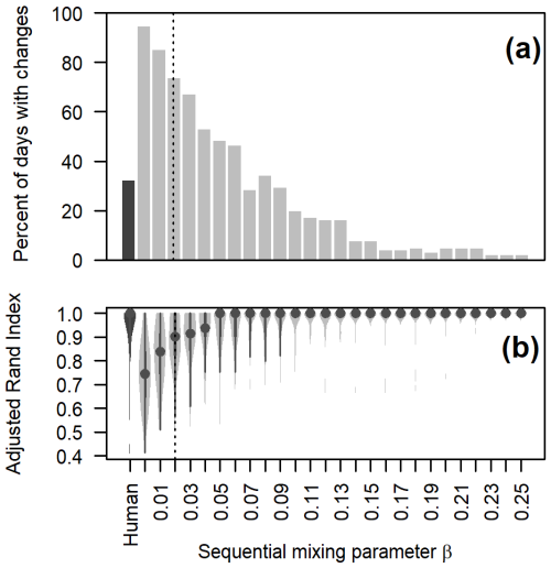
Figure 6 Quantifying changes in clustering results on consecutive days: (a) percent of days when the forecast region arrangements changed and (b) distribution of adjusted Rand index (ARI) values over the season to measure the similarities of clustering results on consecutive days. The leftmost plots display the values for human-assessed forecast regions in dark grey as a benchmark, followed by non-sequential clustering (β=0) and then sequential clustering with β values ranging from 0.01 to 0.25. The violin plot shows the distribution of ARI values with a dot for the median, thick bars for the interquartile range, thin lines for the full range, and light-grey areas for higher data density. The optimal β value chosen for this study was 0.02 (vertical dashed line).

4.4 Sequential weight

We implemented sequential clustering by introducing a sequential weight β that considered the previous day's clustering results. The sequential distance dist_seq was derived from the previous day's clustering membership vectors u_iv. The membership vectors were transformed into a distance matrix using the maximum difference between vector components (supremum norm method). The grid search spanned $\mathit{\beta }=\mathit{\{}\mathrm{0},\mathrm{0.01},\mathrm{\dots },\mathrm{0.25}\mathit{\}}$, ranging from no weight on the previous day (referred to as non-sequential) to 25 % weight. For each β, we applied sequential clustering over the 2022–2023 season using only days when data were available on consecutive days (106 cases). We used the optimal values α=0.25 and $\mathrm{1.2}\le r\le \mathrm{1.3}$ and a fixed k=5 (the median number of human-assessed regions) to remove variability from changing the number of regions over time.

We evaluated the performance of each β value by counting how often forecast regions changed arrangements and measuring the complexity of those changes using the adjusted Rand index (ARI) (Hennig, 2023). The ARI quantifies the similarity between two clustering results: 1 indicates identical groupings, and −1 indicates completely different clusters. The ARI was calculated for clustering solutions on consecutive days to measure the complexity of changes and for the human-assessed forecast regions on the same days, providing a benchmark to assess changes across different β values.

The human-assessed forecast regions changed the arrangement on 32 % of the days with a median ARI of 1.0 over the season, indicating infrequent and simple changes. In contrast, clustering without sequential clustering (β=0) resulted in changes on 94 % of the days with a median ARI of 0.74 over the season, suggesting more frequent and complex changes. Such frequent rearrangement of regions is impractical for operational forecasting, highlighting the need for sequential clustering to stabilize the results.

Applying sequential clustering led to fewer and less drastic changes on consecutive days, especially as β approached 0.25 (Fig. 6). Large values of β forced clustering solutions to converge to a stable solution and removed responsiveness to changing snowpack conditions. We selected β=0.02 to balance result stability with responsiveness to significant changes in snowpack conditions. With β=0.02, the regions changed on 74 % of the days, and the median ARI over the season was 0.90. This represents a midpoint in complexity between human-assessed regions and non-sequential clustering and could be a reasonable workload for forecasters.

5 Clustering results

This section demonstrates the clustering method by applying the optimized parameters from Sect. 4 to both the 2022–2023 and 2023–2024 seasons.

Figure 7 Map of (a) human-assessed forecast regions on 3 February 2023 colour-coded by treeline danger rating (red: 4-High, orange: 3-Considerable, yellow: 2-Moderate) and labelled with avalanche problems in order of importance (SS: storm slab, WS: wind slab, PS: persistent slab, DPS: deep persistent slab). Clustering results for the (b) k=3, (c) k=4, and (d) k=5 regions are shown with subregions colour-coded by their primary cluster membership with greater transparency for low membership values and their membership values labelled. Human-assessed regions are outlined with thick black lines on each map.

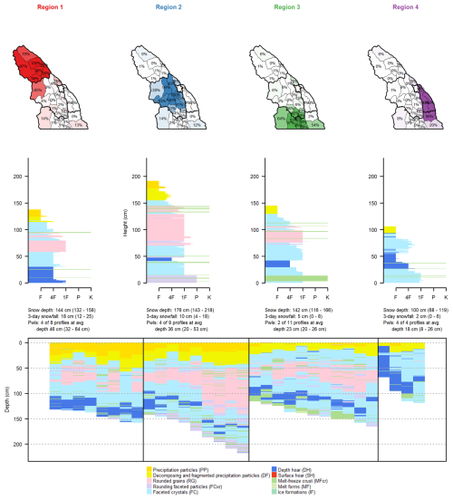
Figure 8 Each region produced with k=4 clustering on 3 February 2023 is shown with a map of the memberships of each subregion in that region (human-assessed regions outlined with thick black lines), an average snow profile from all subregions with membership values above 75 %, a textual summary of snow depth, 3 d snowfall, unstable persistent weak layers (average values are provided first, followed by the minimum and maximum values in parentheses), and, finally, the grain type profiles for all subregions that have the strongest membership in that region.

5.1 Clusters for 3 February 2023

The 3 February 2023 clustering results highlight the method's effectiveness in partitioning meaningful forecast regions. On this day, the Columbia Mountains had four human-assessed forecast regions with varying avalanche hazard conditions (Fig. 7a). The northernmost region had a treeline danger rating of 4-High, while the central region was 3-Considerable and the regions in the south and east were 2-Moderate. Avalanche problems varied across the regions, with storm slabs posing the primary problem in the regions with 4-High and 3-Considerable danger, while wind slabs and deep persistent slabs were the primary problems in regions with 2-Moderate danger. Persistent slabs were the secondary problem in all the regions, with deep persistent slabs also listed as a third problem in the northern and central regions.

The results for $k=\mathit{\{}\mathrm{3},\mathrm{4},\mathrm{5}\mathit{\}}$ demonstrate the clustering method's ability to partition regional patterns at different resolutions (Fig. 7b–d). These regions generally correspond to major avalanche hazard patterns assessed by forecasters. For k=3, regions align with danger rating trends, while k=4 and k=5 further divide areas with 2-Moderate danger, potentially reflecting distinct snowpack conditions and avalanche problems. Fuzzy cluster memberships are most pronounced near regional borders, with some subregions shifting their primary membership as k changes, particularly in southern areas. However, a few subregions also show strong membership values outside their apparent human-assessed regions. The maps of memberships for each cluster region further illustrate how fuzzy analysis clustering can reveal overlapping patterns, as some subregions exhibit similar membership to multiple regions (Fig. 8).

The snow profile characteristics for the k=4 clustering results illustrate the primary factors driving the partitions (Fig. 8). Similar plots for k=3 and k=5 are provided in Appendix B. Distinct snow depth patterns are clear, with deep snowpack areas separated from shallow ones. The northern region (Region 1) had the greatest amount of 3 d snowfall (12 to 25 cm), compared to the central region (Region 2) with 4 to 18 cm and the other regions with less than 8 cm. Greater amounts of 3 d snowfall in the northern and central regions align with their elevated danger ratings and storm slab problems.

All the subregions contain faceted crystals or depth hoar near the bottom of the snowpack (Fig. 8), which aligns with the deep persistent slab problem listed in all regions except the southernmost region. Forecasters did not assess a deep persistent slab problem in the southern region on 3 February because melt–freeze crusts in the upper snowpack reduced the likelihood of triggering. These crusts are present in the simulated profiles. In the eastern region (Region 4), 4 of 4 profiles had unstable persistent weak layers, while the other regions had smaller proportions of unstable persistent weak layers (Region 1: 4 of 8; Region 2: 4 of 9; Region 3: 2 of 11). These proportions align with the fact that deep persistent and persistent slab problems were the most important problems in the eastern region but were secondary problems in the other regions.

5.2 Clusters for different snowpack conditions

Clustering results from several days during the 2023–2024 winter are shown in Fig. 9 to demonstrate the method's ability to partition different types of snowpack conditions. On 3 December 2023, the early-season conditions were split into two regions: one with an average snow depth of 50 cm and the other with 25 cm. The deeper snowpack mostly contained faceted crystals, while the shallower one was dominated by depth hoar. By 3 March 2024, a more complex snowpack had emerged, with large storm snow accumulations, buried melt–freeze crusts, and depth hoar layers, resulting in four distinct regions based on differences in new snow amounts and the presence of crust and depth hoar layers at various depths. By 19 April 2024, the snowpack was transitioning to spring conditions. In the southern regions, the upper snowpack consisted primarily of melt forms and crusts, while the northern regions had fewer melt forms.

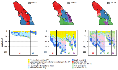
Figure 9 Clustering solutions and snow profiles show the splitting of snow profiles under (a) early-season, (b) mid-winter, and (c) early-spring conditions during the 2023–2024 season. The maps colour-code subregions by their primary cluster membership with greater transparency for low membership. Human-assessed regions on each day are outlined with thick black lines.

Figure 10 Clustering results for each day between 1 January 2024 and 25 April 2024. Subregions within the clusters are colour-coded based on their primary cluster membership, with lower membership values indicated by greater transparency. Human-assessed forecast regions are outlined in black.

5.3 Temporal patterns

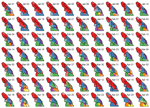
Sequential clustering over the 2023–2024 season resulted in gradual changes in the number and arrangement of forecast regions (Fig. 10). Some subregions formed consistent groupings with high membership values over the season, especially in the northern and central areas. In contrast, the southern and eastern areas were more variable, with changes in the number of regions and some subregions showing consistently low membership values, causing them to shift between regions.

Figure 11 The four most common arrangements of subregions for the 2022–2023 and 2023–2024 seasons according to (a, c) human forecasters and (b, d) clustering results.

5.4 Comparison with human forecast regions

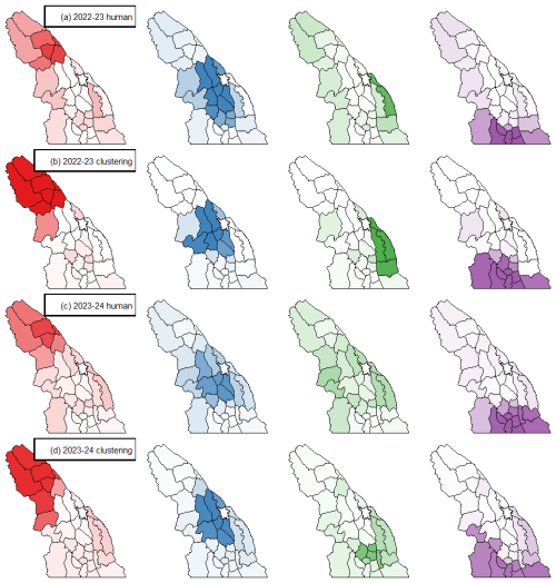
To compare the clustering method's typical forecast regions with the human-assessed regions, we identified common arrangements for each season by counting how often each pair of subregions was grouped together. Using these pairwise counts, we applied the fanny clustering method with k=4 to generate groups representing the four most frequent forecast region arrangements. A larger fuzziness parameter was needed for the count data to handle the large proportion of zero distances, which after optimizing for ASW was found to be r=2.

The clustering method consistently grouped subregions into similar regions to human forecasters each season (Fig. 11). The arrangement of these regions reflects the dominant snow climates in the Columbia Mountains identified by both human forecasters and the clustering method. However, for some specific subregions, there were differences between the clustering and human regions, especially in the southern and eastern parts of the range, where changes to the regions were more frequent for both humans and clustering. Discussions with Avalanche Canada forecasters revealed two main reasons for these differences. First, some of these subregions have limited data availability, leading to lower confidence in forecasters' assessments. Second, some were areas where the operational snowpack model had known accuracy issues, such as underestimating snowfall. Either case could cause inaccurate arrangements, and it is not clear which solutions would better align with reality.

6 Discussion

6.1 Quality of clustering results

The clustering of simulated snow profiles effectively captured major hazard patterns in the Columbia Mountains during the 2022–2023 and 2023–2024 seasons. The clustering of subregions into forecast regions closely aligned with human-assessed regions (Fig. 11). On 3 February 2023, these groupings captured differences in avalanche danger ratings and avalanche problems across the Columbia Mountains (Figs. 7 and 8). The fuzzy analysis clustering method conveyed the inherent uncertainty associated with simulated snow profiles, making it more suitable than a deterministic clustering method. Clustering over the season suggested that the arrangement of forecast regions could change more often than the human-assessed regions.

Our results demonstrate the method's potential for avalanche forecasting but with several limitations. It was tested in only one mountain range over two seasons, limiting its generalizability across different snow climates and regions. While we did not conduct comprehensive cross-validation under varied conditions, it is encouraging that the method performed similarly in both seasons, despite the parameters being tuned using data from only one season.

Comparisons with human-assessed regions provide only limited insight due to inherent uncertainties in their assessments. Also, forecasters may have been influenced by viewing the same simulated snow profiles on their operational snowpack model dashboard, which included a prototype clustering product. This product used a simplified snow profile distance metric, a larger domain, hierarchical clustering, and different validation metrics for determining the number of clusters. This dashboard was likely used more in remote regions where field observations are less abundant than in the Columbia Mountains.

6.2 Practical avalanche forecasting considerations

Clustering could help forecasters identify spatial patterns in complex datasets such as snowpack model simulations. While a similar approach could be applied to traditional field observations, spatially distributed snowpack simulations provide the advantage of continuous spatial and temporal coverage.

The operational snowpack model used in this study was primarily configured to predict avalanche problems associated with new snow and persistent weak layers and did not account for aspect-specific conditions. Consequently, the snow profile distance metric dist_pro emphasized these specific snow profile characteristics. However, this distance metric could be changed to incorporate other relevant snowpack characteristics, such as those associated with wind slab or wet snow problems.

The clustering results presented here focus on regional-scale patterns, as the rows and columns in the distance matrix represent entire subregions. However, the concept of spatial constraints can be extended to other spatial scales by adapting the distance metric dist_geo to quantify other types of spatial relationships. For example, dist_geo could be redefined to quantify relationships between different aspects and elevation bands or between profiles distributed across a single slope. Integrating aspect and elevation bands into the clustering analysis would enable a more comprehensive representation of the spatial scales relevant to regional forecasters and is particularly important for wind and wet snow problems. For example, Bouchayer (2017) demonstrated that the clustering of simulated snow profiles on a 1.3 km grid in France revealed local-scale snowpack patterns and elevation effects, highlighting the potential of incorporating more spatial considerations into clustering analyses.

While clustering offers insights into complex model output, forecasters should treat them with some level of caution. Due to the challenge of validating the accuracy of spatially distributed snowpack simulations, we currently do not recommend using this clustering method for unsupervised automation. Instead, forecasters should consider clustering as a data exploration tool. For example, forecasters could adjust the number of regions k to view clustering results at different resolutions and gain insights into potential hazard patterns.

6.3 Technical considerations for snow profile clustering

A critical aspect of this clustering method was the distance metric used to compare snow profile characteristics, which took advantage of the recent developments of Herla et al. (2022) and Mayer et al. (2022). Condensing snow profile comparisons into a single numerical value is inherently challenging and represents a serious simplification. Hence, careful consideration must be given to quantifying the snow profile distance, given the impact it can have on clustering results. Deriving a meaningful snow profile similarity metric for Herla et al. (2022) and this study required careful trial and error to properly weigh relevant snowpack features.

The distance between subregions (dist) can easily be integrated into other clustering methods such as hierarchical clustering or partition-based methods like k-means and k-medoids. Hierarchical clustering generates intuitive tree-like structures with nested clusters, visualizing patterns at different resolutions. Herla et al. (2021) presented a simple example of hierarchical clustering of snow profiles. An enhancement of k-means clustering could involve applying dynamic barycenter averaging to define cluster centroids (Petitjean et al., 2011), as Herla et al. (2022) recently adapted this method for snow profiles. Additionally, clustering simple scalar indices derived from snow profiles would be more computationally efficient than evaluating the entire snow stratigraphy. For example, Reuter et al. (2023) derived avalanche problem types from simulated snow profiles and clustered their frequencies to predict snow climatologies.

Selecting parameters for a clustering method must be done with care for each application. Section 4 presents possible approaches for tuning parameters to new datasets. Factors such as the variability within a snow profile dataset, the number of subregions, and the spatial arrangement will influence parameter selection. Recent attempts to apply this method across the larger domain of western Canada suggest that the parameters may need retuning to accommodate other datasets, as would applications in other climates and countries. Tuning parameters to make the clustering results align with human-derived forecast regions proved to be helpful.

Computational time is a critical consideration for operationalizing clustering methods. While computing pairwise similarities for a small number of profiles is relatively efficient, scalability becomes an issue with larger datasets. Applying different clustering methods or changing k is relatively fast after computing the distance matrix. Real-time applications should consider code optimization and parallelization to manage computational demands efficiently.

7 Conclusions

Statistical clustering offers a valuable approach for identifying avalanche hazard patterns within complex snowpack model datasets. This study shows the effectiveness of a clustering method that accounts for spatial and temporal trends, as the major patterns across the Columbia Mountains during two winter seasons closely aligned with human-assessed forecast regions. The application of fuzzy analysis clustering facilitates the representation of uncertainty in simulated snow profiles, providing nuanced insights for forecasters. Adjusting the number of clusters can reveal patterns at various levels of spatial resolution.

These methods can adapt to consider different criteria, such as different snowpack characteristics or spatial relationships. With numerical snowpack modelling advancing rapidly, forecasters need intuitive tools to explore model outputs. Avalanche Canada plans to implement and refine these methods in their operational snowpack model system. Embracing clustering as a form of exploratory data analysis should enhance the interpretability of snowpack model outputs and support more informed decision-making in avalanche forecasting.

Appendix A: Configuration of operational modelling system

This Appendix summarizes Avalanche Canada's operational snowpack modelling system for the 2022–2023 and 2023–2024 seasons (Horton et al., 2023). The system forced SNOWPACK version 3.4.5 (Lehning et al., 1999) with meteorological data from two numerical weather prediction (NWP) models run by Environment and Climate Change Canada: the High-Resolution Deterministic Prediction System (2.5 km horizontal resolution) and the Regional Deterministic Prediction System (15 km resolution) (Milbrandt et al., 2016).

To capture regional-scale patterns across large forecast regions, the system selected representative grid points from each NWP model with a stratified sampling approach to balance spatial resolution and computation costs. Forecast subregion polygons were divided into small microregion polygons with typical areas of 300 to 600 km² each. Within each microregion, alpine, treeline, and below-treeline elevation grid points were sampled from each NWP model (depending on whether the actual and modelled terrain extended to that elevation). This study used 168 treeline elevation grid points, including 126 from the high-resolution NWP model and 42 from the regional model (Fig. 1a). Information from both models is combined when averaging the snow profiles, with the higher number of high-resolution model points typically dominating the average in most subregions.

Hourly time series data for precipitation amount, precipitation type, air temperature, humidity, wind speed, incoming shortwave radiation, and incoming longwave radiation were compiled 6 h at a time from each successive NWP model run to generate the necessary meteorological forcings for SNOWPACK. SNOWPACK was configured to simulate flat field snow profiles with wind transport disabled, ensuring that simulations represented widespread regional snowpack characteristics.

As part of the operational model, snow depth observations were assimilated weekly following a method based on Horton and Haegeli (2022). The method compares changes in modelled snow depth over the previous week with changes observed at nearby sites (i.e., automated weather stations and manual observations by avalanche professionals). Snow depth observations from these sites were lapse-rate-adjusted to local treeline elevations and then spatially interpolated to the model grid points. Potential errors in snowfall amounts were identified by comparing modelled snow depth increases over the past week with increases in interpolated observations. Cases where either the modelled or observed snow depth increased by more than 10 cm were identified, and then corrective action was taken if the increases differed by more than 10 %. Specifically, SNOWPACK was rerun with the input precipitation amount adjusted by a constant factor to nudge the modelled snow depth towards observed values.

Simulated snow profiles were stored in a database, which fed an online visualization dashboard used by operational avalanche forecasters. For this study, we queried a subset of profiles from this database.

Appendix B: Clustering results on 3 February 2024 for other values of k

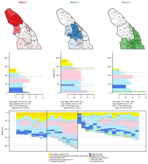
Figure B1 Comparison of regions produced with clustering results for k=3 on 3 February 2023. Each column shows a region with a map of the memberships of each subregion of that region; an average snow profile from all subregions with membership values above 75 %; a textual summary of snow depth, 3 d snowfall, and unstable persistent weak layers (average values are provided first, followed by the minimum and maximum values in parentheses); and, finally, the grain type profiles for all subregions belonging to that region.

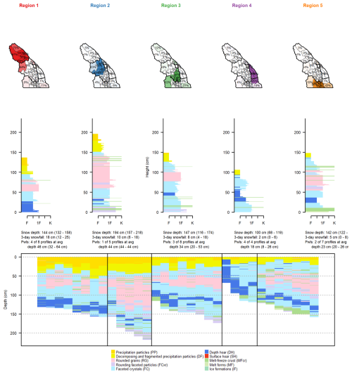
Figure B2 Comparison of regions produced with clustering results for k=5 on 3 February 2023. Each column shows a region with a map of the memberships of each subregion of that region; an average snow profile from all subregions with membership values above 75 %; a textual summary of snow depth, 3 d snowfall, and unstable persistent weak layers (average values are provided first, followed by the minimum and maximum values in parentheses); and, finally, the grain type profiles for all subregions belonging to that region.