Indian Institute of Tropical Meteorology (IITM) High-Resolution Global Forecast Model version 1: an attempt to resolve monsoon prediction deadlock

The prediction of Indian monsoon rainfall variability, affecting a country with a population of billions, remained one of the major challenges of the numerical weather prediction community. While in recent years, there has been a significant improvement in the prediction of the synoptic-scale transients associated with the monsoon circulation, the intricacies of rainfall variability remained a challenge. Here, an attempt is made to develop a global model using a dynamic core of a cubic octahedral grid that provides a higher resolution of 6.5 km over the global tropics. This high-resolution model has been developed to resolve the monsoon convection. Reforecasts with the Indian Institute of Tropical Meteorology (IITM) High-Resolution Global Forecast Model (HGFM) have been run daily from June through September 2022. HGFM has a wavenumber truncation of 1534 in the cubic octahedral grid. The monsoon events have been predicted with a 10 d lead time. HGFM is compared to the operational Global Forecast System (GFS) T1534. While HGFM provides skills comparable to GFS, it shows better skills for higher precipitation thresholds. This model is currently being run in experimental mode and will be made operational.

1 Introduction

In spite of significant improvement in numerical weather prediction skill in the last decades (Bechtold et al., 2008; Magnusson and Kallen, 2013; Hoffman et al., 2018), predictions of tropical rainfall variability remain a challenge (Westra et al., 2014; Prakash et al., 2016). Stephens et al. (2010) demonstrated that the models predict too many rainy days in the tropics, which are in the lighter rain category. The challenges of tropical rainfall variability have also been demonstrated by Watson et al. (2017). The vagaries of the Indian monsoon every year affect the lifestyle of billions of people and affect the economy of the Indian subcontinent, modulating its gross domestic product (GDP) (Gadgil and Gadgil, 2006). It is, therefore, of the utmost importance to improve the weather prediction skill in general and extreme precipitation event prediction in particular. With the increase in computing power, the resolution of numerical weather prediction models has been increasing, and global models with a resolution of 1–7 km have become a reality (Majewski et al., 2002; Satoh et al., 2005; Miura et al., 2007; Staniforth and Thuburn, 2012; Li et al., 2015; Satoh et al., 2019; Wedi et al., 2020). The higher resolution of numerical weather prediction (NWP) models has been found to produce realistic rainfall variability across various scales, including better diurnal variation, Madden–Julian Oscillation (MJO) variability, and seasonal mean climate (Kinter et al., 2013; Rajendran et al., 2008; Skamarock et al., 2012; Molod et al., 2015; Crueger et al., 2018; Giorgetta et al., 2018). In India, operational NWP was initiated with a moderate resolution of T80 and then gradually enhanced to T382 and T574 (Prasad et al., 2011, 2014, 2017) and very recently to T1534 (Mukhopadhyay et al., 2019). The advantage of using a higher resolution (T1534 ∼ 12.5 km) vs. a lower resolution T574 (∼ 27 km) was found by the enhancement of the model skill by 2 d (Rao et al., 2019). The National Center for Environmental Prediction (NCEP) Global Forecast System (GFS) model with 21 members has been used for probabilistic forecasts since June 2018 (Deshpande et al., 2021). The high-resolution GFS T1534 was found to enhance the skill in predicting heavy-rainfall events (Mukhopadhyay et al., 2019), tropical cyclones, and even block-level rainfall (a block is a subdivision of the district in India, typically the size of the grid of GFS T1534). However, the skill of the GFS T1534 for the prediction of extremely heavy precipitation can still be improved, particularly over the orographic regions of India such as the southern coastal state of Kerala (Mukhopadhyay et al., 2021).

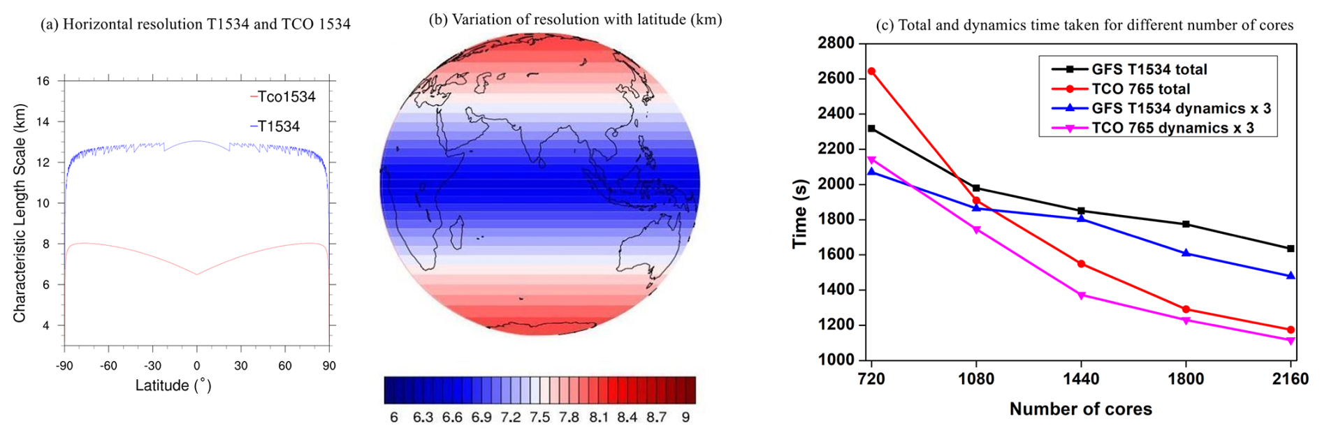
Figure 1 Variation in grid length with latitude in GFS (blue) and Tco (red) (a). A depiction of grid resolution over the globe in the Tco grid (b). The total and dynamics time taken for different numbers of cores (c): the time taken by GFS and HGFM for a 1 d forecast (the y axis is the total time taken and the model dynamics time multiplied by 3).

The 12 km deterministic model and the ensemble model based on the GFS show reasonably good skill in capturing the monsoon rainfall with 3 to 5 d lead time. The skill of the GFS forecast for the Indian monsoon has been reported by Mukhopadhyay et al. (2019), and the skill at predicting tropical cyclones with the Global Ensemble Forecast System (GEFS) has also been reported by Deshpande et al. (2021) and Kanase et al. (2023). However, in a recent study, Mukhopadhyay et al. (2021) showed that three state-of-the-art ensemble forecast systems, namely the GEFS, the United Kingdom Meteorological Office (UKMO)-based NCMRWF Ensemble Prediction System (NEPS) run by the National Centre for Medium Range Weather Forecasting (NCMRWF), and the Integrated Forecasting System (IFS) by ECMWF struggled to capture the extremely heavy rainfall over Kerala during the August 2018 and August 2019 extremely heavy-rainfall episodes. This, in fact, has shown the limitations of the model in resolving the rainfall variability over the Indian region and, more importantly, over the orographic region. One of the limitations in resolving the regional variabilities in rainfall is the horizontal resolution, which does not allow the model to resolve the smaller-scale processes. Therefore, a need was felt to enhance the horizontal resolution of the existing GFS-based forecasting system. As running a model close to the convection-permitting model (at a resolution lesser than 10 km) is too computationally expensive in conventional reduced Gaussian linear grids, we instead built a weather model with a grid that has a variable resolution from the pole to the Equator. In view of this, the GFS reduced Gaussian linear grid at triangular truncation 1534 is replaced by an equivalent truncation of 1534 in a triangular–cubic–octahedral (Tco) grid. The equivalent model resolutions of the linear T1534 and the cubic Tco1543 grids are displayed in Fig. 1a. The linear grid has a roughly uniform grid point resolution of 12.5 km; the octahedral grid has a resolution of about 8 km in the polar regions and around 6 km in the tropical band. One of the prominent examples of a global NWP model with the Tco grid is that of the European Centre for Medium-Range Weather Forecasts (ECMWF) model suites. The Tco grid provides several advantages (ECMWF Documentation Cy43r1, 2016) over that of the conventional reduced Gaussian linear grid (Fig. 1a), i.e., a significant reduction in computation cost, improved representation of orography, better filtering, and better conservation properties. These properties of Tco make it a better candidate, particularly for use on high-performance computing (HPC).

To the best of our knowledge, this paper is the first attempt at building a model close to a convection-permitting global weather model in India, with an emphasis on Indian monsoon rainfall variability. The details of the model development and the experiments conducted have been elaborated in Sect. 2. The model results are analyzed in Sect. 3, and the conclusion of the study is summarized in Sect. 4.

2 Model, data, and methodology

This new grid, namely the triangular–cubic–octahedral (Tco) grid, has been adopted to change the existing GFS (semi-Lagrangian) Gaussian linear model system. In the spectral domain, dynamical fields are represented by the sum of spherical harmonics. The total wavenumber characterizes the spherical harmonics, and the associated wavelength is the ratio of the circumference of the Earth to the total wavenumber. The value of the maximum wavenumber (n_max) used to represent a field as the sum of spherical harmonics is also the spectral truncation of the model. In the case of both GFS and Tco, the value of n_max is 1534. For the same spectral truncation n_max, the number of latitude circles from the Equator to the pole can vary depending on the choice of spectral transformation. For a linear grid, n_max = 2N−1 and for a cubic grid, n_max = N−1. Therefore, for a linear Gaussian grid, the smallest wavelength is represented by only two grid points, as is the case with the GFS T1534 model. However, in the case of triangular truncation, the smallest wavelength is represented by four grid points (in the case of the Tco grid). In triangular truncation, for the same spectral truncation, the number of latitude circles is about double that of the linear truncation. For the GFS model, the horizontal resolution is ∼ 12.5 km, and applying the cubic grid ensures that the horizontal resolution becomes ∼ 6.5 km in the tropics (about half of the model resolution that is currently used) for the Tco grid. In the Tco grid, the number of latitude circles is 1535.

Once a particular choice of spectral truncation is made, the number of latitude circles becomes obvious. However, the number of longitude circles per latitude circle remains to be prescribed to create the global grid structure. In a fully Gaussian grid, the number of longitude circles per latitude circle remains the same throughout the latitudes from the Equator to the poles. Thus, the effective resolution near the poles becomes very high compared to the equatorial regions. This specific requirement demands too many computational resources and poses numerical instability problems. To overcome that issue, in the linear Gaussian grid, the number of latitude circles decreases in a certain way from the Equator toward the poles to ensure almost the same zonal resolution. For the cubic–octahedral grid, the number of longitude points per latitude circle is prescribed differently. The latitude circle closest to the pole consists of 20 longitude points, and the number of longitude points increases by 4 at each latitude circle, moving from the poles towards the Equator. The number of longitude points at the Equator in the case of the Tco grid is given by $N_x=\mathrm{20}+\mathrm{1534}\times \mathrm{4}=\mathrm{6156}$. Therefore, the zonal grid length = $\mathrm{2}\mathit{\pi }\times R/N_x\sim$ 6.5 km. In the original reduced Gaussian grid, the number of longitude points per latitude point remains fixed in different blocks of latitudes. The number of latitude points jumps from one block to another by a constant number. Unlike the linear reduced Gaussian grid, the horizontal resolution varies more smoothly with latitude in Tco. The Collignon projection of a sphere projects this configuration onto an octahedron. In the current study, the Tco grid at the truncation wavenumber of 1534 is used. This new version of the model is called HGFM (High-Resolution Global Forecast Model version 1) throughout the paper. Figure 1a and b depict the variation in grid resolution with latitude in the semi-Lagrangian (SL) GFS and HGFM (Tco). Details about the model code can be found in Phani et al. (2024a).

Table 1 Details of the domain configuration and physics options used in HGFM.

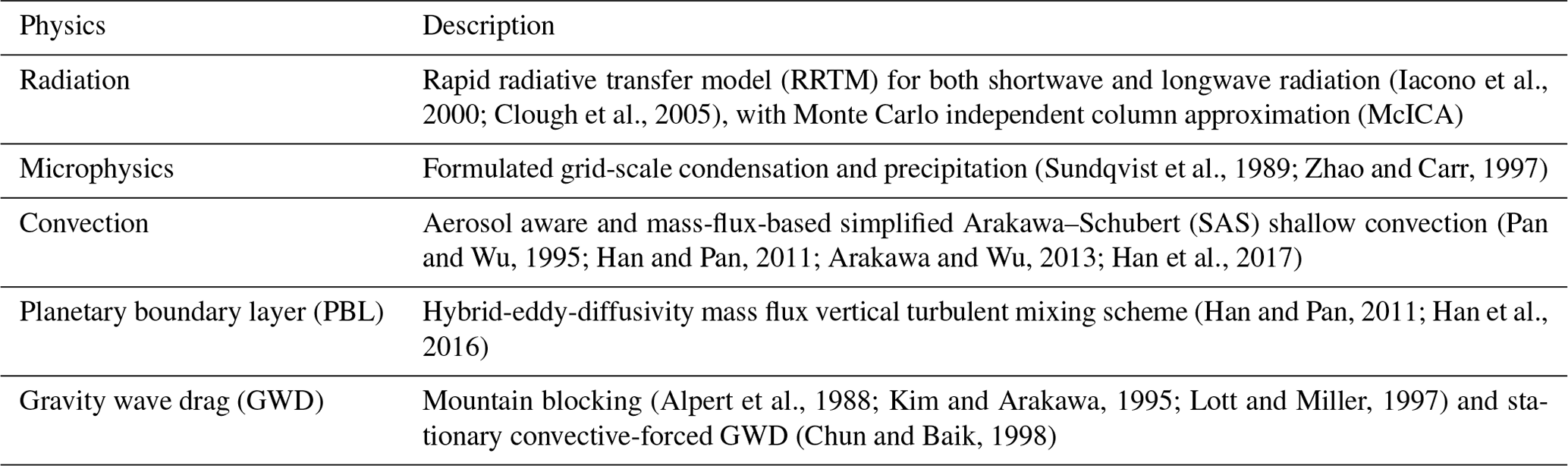
Before testing HGFM with complete physics (see Table 1 for a description of physics used in both versions of the model), we developed a version of HGFM with only a dynamical core, following the approach of Held and Suarez (1994) referred to as HS94. HS94 was run to check the stability of the Tco grid framework. Surface boundary conditions for the Tco grid were meticulously prepared to ensure the accuracy of grid point representation. Moreover, HGFM (Tco1534) was developed with complete physics and incorporates essential boundary conditions including global topography, global land use land cover, etc. HGFM at the Tco1534 truncation is depicted over the globe in Fig. 1. The model has been run daily for a 10 d forecast at the Indian Institute of Tropical Meteorology (IITM) Pratyush high-performance computing (HPC) system. To understand the computational efficiency of the Tco model, the time taken for a 1 d forecast is compared for GFS T1534 and HGFM (Tco765 in this case; see Fig. 1c). A comparison between GFS T1534 and Tco765 is made because both models have nearly the same number of grid points. It is evident that Tco765 significantly saves runtime in dynamical cores and saves total time as well. Moreover, the Tco model is in general more scalable for a higher number of cores (not shown). The model has been running since 2022, and here, the analyses for the summer monsoon season of June, July, August, and September (JJAS) 2022 are presented (Phani et al., 2024b). A detailed analysis of the model run is discussed in the results section. Apart from the monsoon season (JJAS 2022), a few case studies are also discussed.

To verify the model forecast, the daily observed gridded rainfall data from IMERG (Integrated Multi-satellite Retrievals for GPM (Global Precipitation Measurement)) version 06B (Huffman et al., 2019) rainfall data at a 0.1° × 0.1° (10 km) horizontal resolution are utilized for the JJAS season of the year 2022. Additionally, for the validation of a heavy-rainfall event over India, gridded rainfall data from the India Meteorological Department (IMD) at a 25 km resolution are used. The IMD rainfall data are a merged product of gridded rain gauge observations and GPM satellite-estimated rainfall over the Indian summer monsoon (ISM) region (Mitra et al., 2014). Further, the reanalysis-based parameters from the fifth generation of ECMWF atmospheric reanalysis (ERA5) products (Hersbach and Dee, 2016) at a 25 km horizontal resolution are utilized during the JJAS season of the year 2022.

3 Results and discussions

3.1 200 hPa kinetic energy spectra

Before going into the details of model validation, the first metric to evaluate the model fidelity is to validate the kinetic energy (KE) spectra of 200 hPa wind. The KE spectra provide information about the distribution of kinetic energy across scales. A close resemblance between observed/reanalysis-based spectra and spectra produced by the model gives confidence about the accuracy of overall model configuration. The kinetic energy (KE) spectrum in the upper troposphere exhibits two clearly defined power-law patterns. Observational studies have established that at the large scale, rotational modes prevail (k⁻³), while at mesoscales, divergent modes are dominant ($k^{-\mathrm{5}/\mathrm{3}}$) (Nastrom and Gage, 1985). Figure 2 shows the KE spectra of 200 hPa wind simulated by HGFM and GFS T1534. The KE spectra for the forecast with up to 3 d lead time have been compared with ERA5 data. While both the models capture $k^{-\mathrm{5}/\mathrm{3}}$ behavior of the mesoscale reasonably well at the higher wavenumber, HGFM appears to capture the k⁻³ behavior of the large scale at the lower wavenumber in a way that is closer to observations. It is observed that beyond wavenumber 10⁻⁴, there is a slight departure of the spectra from observations, especially for HGFM. However, the regions of interest in KE spectra are the k⁻³ dependence for the large scale and a less steep $k^{-\mathrm{5}/\mathrm{3}}$ dependence for the mesoscale. The tails of the spectra at higher wavenumbers typically have less energy due to the dissipation of kinetic energy with an increase in wavenumber. However, models tend to dissipate the energy at higher wavenumbers at a much faster rate depending on the damping used in the model (Skamarock, 2004). To keep the spectra realistic, a common practice is to reduce the damping, which may increase the energy at higher wavenumbers, as observed in this case for HGFM. However, this will not have much impact on our analysis, as these are the small-scale features. The KE spectra indicate that the overall configuration of both versions of the model is robust. Therefore, we now turn our attention towards verification of convective available potential energy and rainfall simulations, the most desirable parameters in model forecasts.

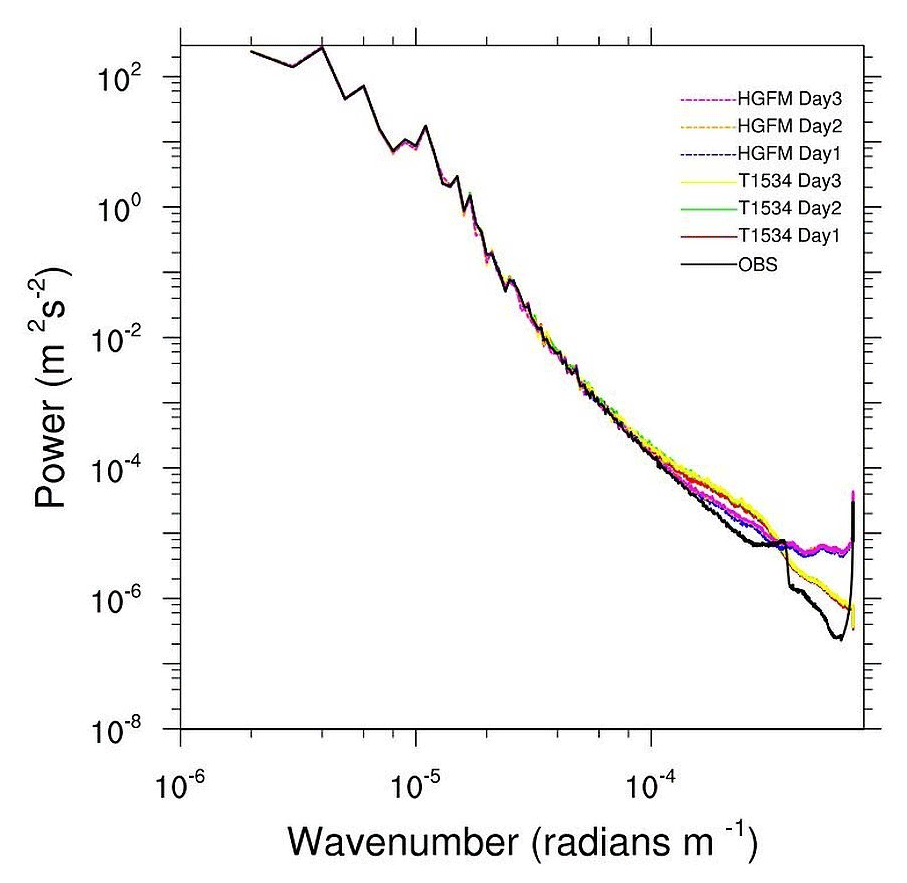
Figure 2 Kinetic energy spectra of 200 hPa wind for observations and for different lead times of GFS T1534 and HGFM.

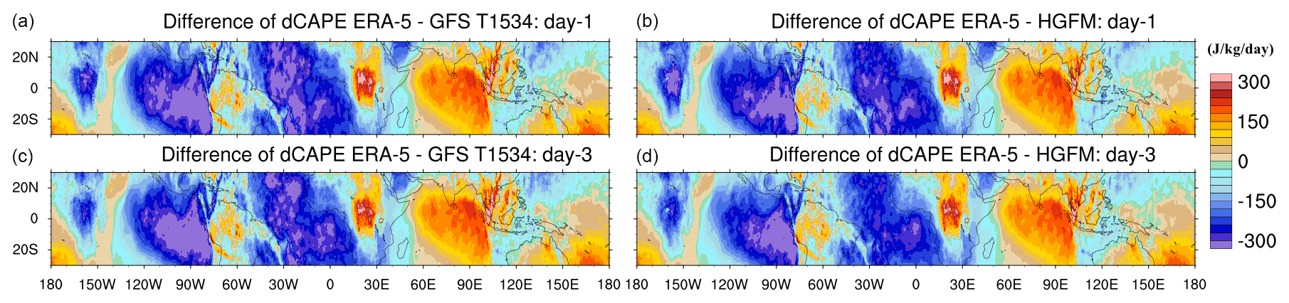
Figure 3 The difference in dCAPE between ERA5 and GFS T1534 for 1 d and 3 d lead times (a, c) and between ERA5 and HGFM for 1 d and 3 d lead times (b, d).

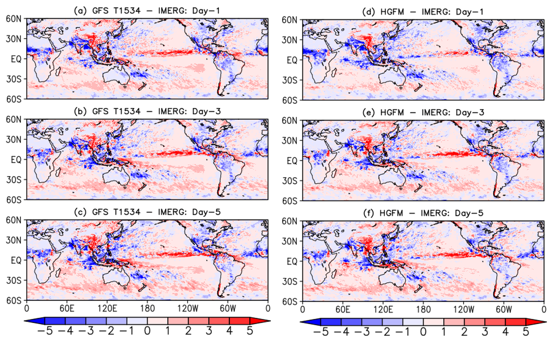
Figure 4 Global JJAS precipitation bias (cm d⁻¹) of GFS T1534 (a–c) with respect to IMERG for (a) 1 d, (b) 3 d, and (c) 5 d lead times. The right column (d–f) indicates similar plots but for HGFM.

3.2 Quasi-equilibrium in models

Both model versions are run at high resolutions, close to convection-permitting model resolutions. However, in this case, a scale-aware convection scheme is used to parameterize deep convection in the model. Observational studies have established that the tropical atmosphere deviates significantly from the convective quasi-equilibrium (e.g., Zhang, 2003). The convective quasi-equilibrium (CQE) is the fundamental approach used in most models for the parameterization of deep convection (Arakawa and Schubert, 1974). To understand the extent to which both model versions obey CQE, we adopted the methodology suggested by Kumar et al. (2022). The absolute value of changes in convective available potential energy (CAPE) at daily timescales (dCAPE) is analyzed using GFS T1534 and HGFM for the year 2022 during JJAS and compared with the ERA5 data (figure not shown). Notable changes were observed in the dCAPE values between GFS T1534 and HGFM compared to ERA5. The dCAPE values from ERA5 data match better with HGFM than GFS T1534 for 1 d and 3 d lead times. The difference in dCAPE between ERA5 and models is presented for 1 d and 3 d lead time forecasts (Fig. 3). The dCAPE differences quantified by ERA5 with GFS T1534 were −49.0570 and −47.3799 $\mathrm{J}{\mathrm{kg}}^{-\mathrm{1}}{\mathrm{d}}^{-\mathrm{1}}$ for 1 d and 3 d lead times, respectively. Similarly, with HGFM, the values were −49.1278 and −43.7668 $\mathrm{J}{\mathrm{kg}}^{-\mathrm{1}}{\mathrm{d}}^{-\mathrm{1}}$ for 1 d and 3 d lead times, respectively.

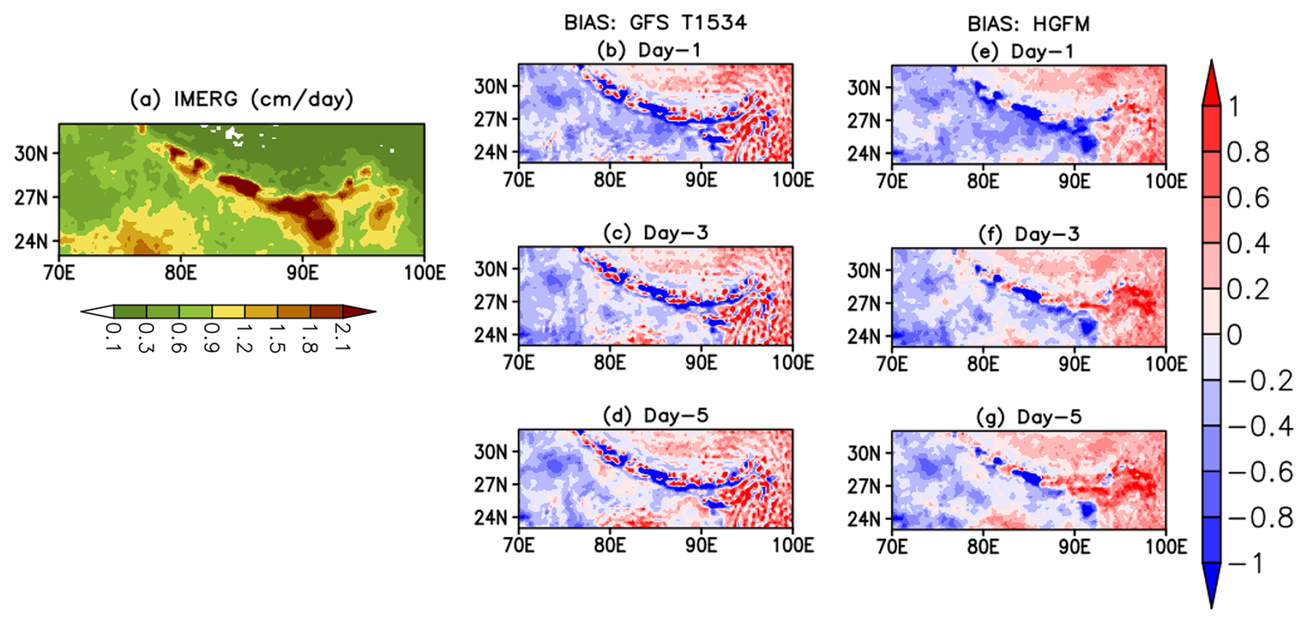
Figure 5 Comparison of JJAS mean precipitation (cm d⁻¹) and bias in IMERG data (cm d⁻¹) (a) with GFS T1534 (b–d) and Tco1534 (e–g) in the year 2022 over the Himalayan foothills and northeast India for 1 d, 3 d, and 5 d lead times.

3.3 Analysis of global precipitation

The global precipitation bias of GFS (left panel of Fig. 4) and HGFM (right panel) with respect to Integrated Multi-satellite Retrievals for GPM (IMERG) data with 1 d, 3 d, and 5 d lead times is shown in Fig. 4. Both the models broadly show a similar rainfall bias over the global land and global ocean. However, there are some subtle differences. The 1 d forecast (Fig. 4a) of GFS shows a wet bias over the equatorial eastern Pacific extending up to the tropical western Pacific. On the other hand, HGFM with a 1 d lead (Fig. 4d) also shows a wet bias mostly confined to the tropical eastern Pacific and also shows a slight negative bias over the western Pacific. For HGFM, the positive bias in rainfall over the tropical ocean appears to be mainly over the eastern Pacific, while that of GFS appears to extend from the eastern Pacific towards the central and western Pacific for all lead times. The eastern Pacific precipitation overestimation could be due to improper representation of shallow convection over the region. Raymond (2017) highlighted the complex nature of sea surface temperature (SST) and associated cloudiness and convection over the region. Apart from the oceanic region, the major global land regions (central African continent, Maritime Continent, Indian summer monsoon region, and northern part of South America) show a negative bias in both models at different lead times (Fig. 4), which is likely related to the model's physical parameterizations.

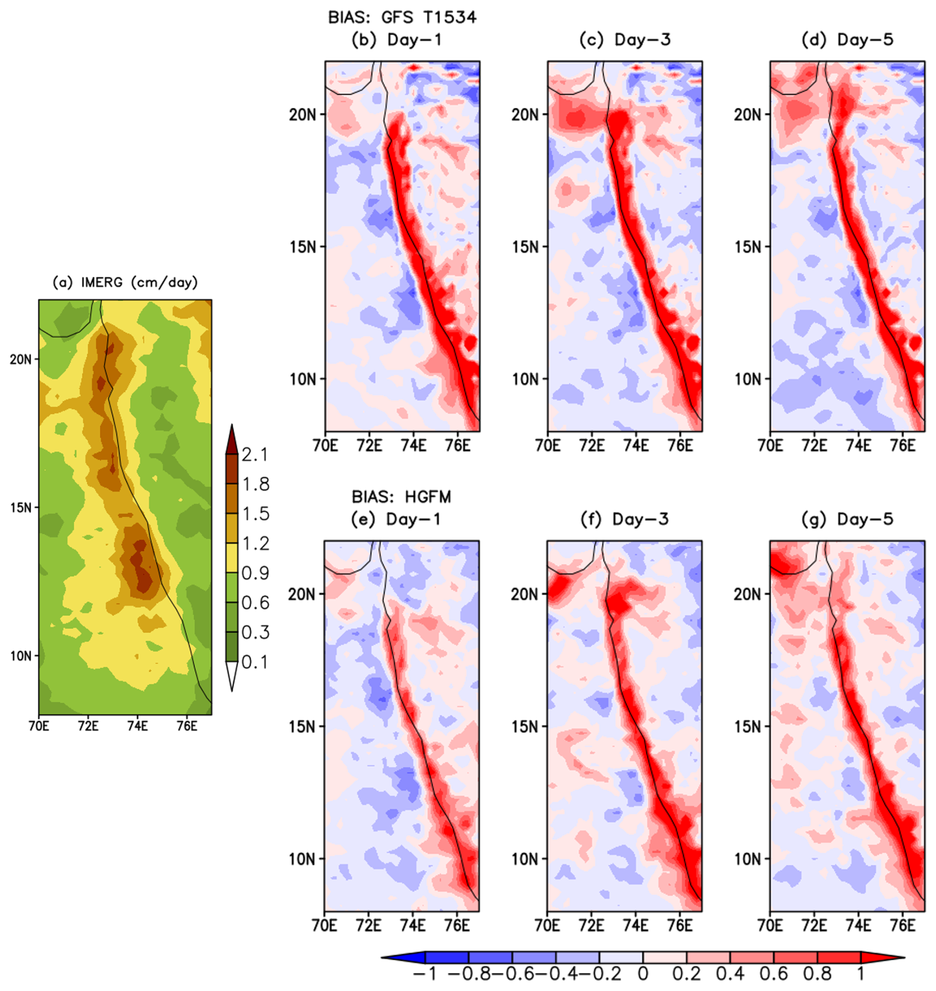
Figure 6 Comparison of JJAS mean precipitation (cm d⁻¹) and bias in IMERG data (cm d⁻¹) (a) with GFS T1534 (b–d) and Tco1534 (e–g) in the year 2022 over the Western Ghats region for 1 d, 3 d, and 5 d lead time.

3.4 Indian summer monsoon precipitation and related features

While Fig. 4 depicted the precipitation bias over the global domain, it will be interesting to investigate the model forecast performance over the complex orographic region over the Indian domain, the region of our ultimate interest. As mentioned earlier, one of the major advantages of using a Tco grid is that it better represents orography. Therefore, it is imperative to investigate the forecast skill of HGFM over the mountainous Himalayan foothills adjoining northeast India and the Western Ghats (WG) region (shown in Figs. 5 and 6, respectively). The GFS T1534 model forecasts indicate spurious rainfall activity over the Himalayan foothills and northeast Indian region for all lead times (Fig. 5b–d). On the contrary, HGFM with a finer horizontal resolution largely resolves the spurious rainfall over the region, as shown in Fig. 5e–g. The Gibbs waves are largely suppressed over the mountainous terrains in HGFM compared to GFS T1534. Similarly, the precipitation distribution over the WG region shows considerable overestimation in GFS T1534 for all lead times (Fig. 6b–d). On the other hand, the magnitude of overestimation is decreased considerably in HGFM forecasts, as depicted in Fig. 6e–g. Thus, the above analysis highlights the fact that HGFM shows its potential in predicting realistic rainfall distribution over the orographic regions.

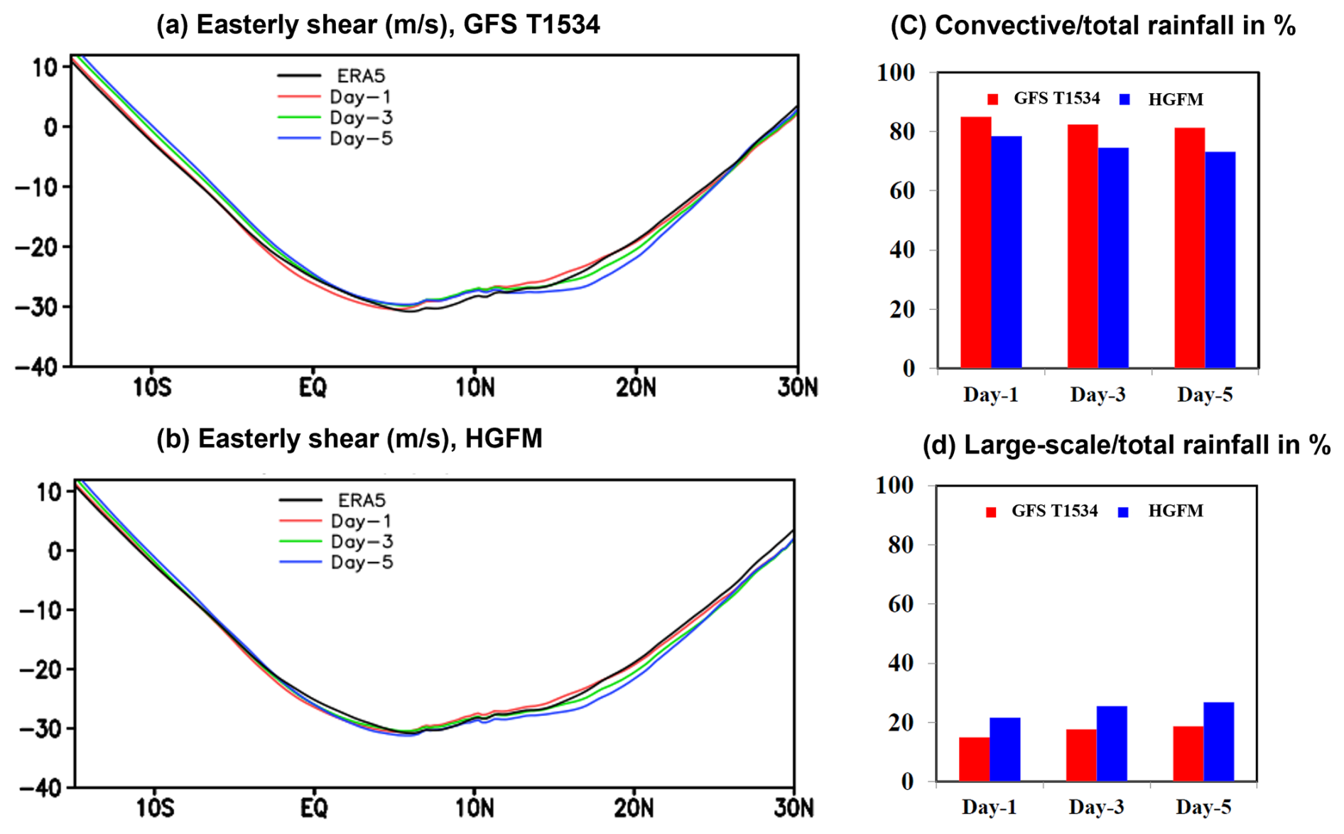
Figure 7 Comparison of easterly shear (m s⁻¹) from ERA5 with GFS T1534 (a) and HGFM (b), along with convective/total rainfall (c) and large-scale/total rainfall (d) between GFS T1534 and HGFM during JJAS 2022, for 1 d, 3 d, and 5 d lead times.

One of the prominent features of ISM is the vertical shear of zonal wind. Previous studies (Jiang et al., 2004; Abhik et al., 2013) demonstrated that the vertical easterly wind shear plays a crucial role in inducing baroclinic vorticity ahead of the northward propagation of summer intraseasonal oscillation. To assess the model forecast skill in predicting realistic easterly wind shear (the difference between zonal wind at 200 and 850 hPa) during the summer monsoon season of 2022, the vertical wind shear is calculated and is represented in Fig. 7a and b for GFS T1534 and HGFM, respectively, over the ISM region. Figure. 7a indicates slightly weaker easterly shear in GFS T1534 compared to ERA5 around 10° N and 0–15° S for all lead times. On the contrary, HGFM predicts more realistic easterly wind shear over the above regions, as shown in Fig. 7b. It is noticeable that both models overestimate the magnitude of easterly shear around 20° N for 3 d and 5 d lead times.

Another key feature of tropical precipitation is the almost equipartition of rainfall into convective and stratiform rain. Therefore, it is important to investigate whether the relative improvement in the precipitation distribution over the ISM region in HGFM forecasts is contributed by improved convective and large-scale precipitation. The model-forecasted convective and large-scale rainfall ratios are shown in Fig. 7c and d, respectively. It is noteworthy that the large-scale or stratiform rainfall plays an important role in the propagation and maintenance of the tropical intraseasonal convection, which is associated with its top-heavy heating profile (Fu and Wang, 2004; Chattopadhyay et al., 2009; Deng et al., 2015). The heating profile associated with stratiform rain also helps in the large-scale organization of convection (see, for example, Choudhury and Krishnan, 2011; Kumar et al., 2017). The contribution of convective rainfall to the total rainfall appears to be more than 80 % in GFS T1534 forecasts for all lead times (Fig. 7c). A similar overestimation of convective rainfall in GFS T1534 is reported by Ganai et al. (2021). The observed convective (large-scale) rainfall ratio is around 55 % (45 %), as shown in Abhik et al. (2017). The HGFM forecast shows relative improvement in predicting convective and large-scale rainfall ratios compared to GFS T1534 (Fig. 7c and d). The decrease (increase) in the convective (large-scale) rainfall contribution to total rain is noted in the HGFM forecast. The finer horizontal resolution of HGFM possibly allows for a more accurate representation of deep convection due to scale-aware representation.

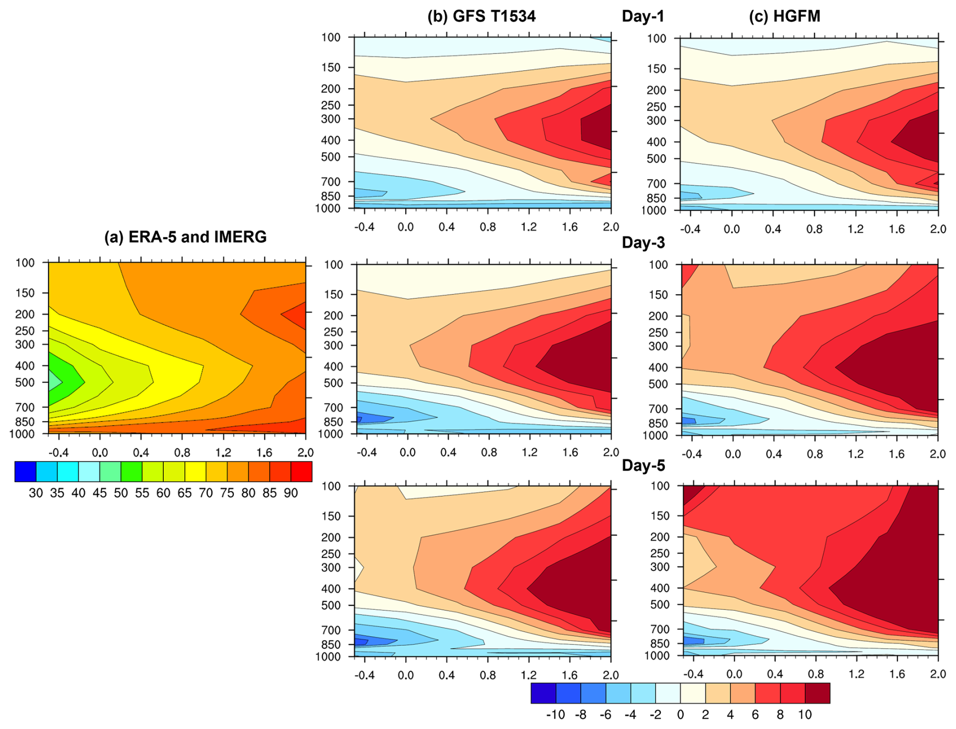
Figure 8 Comparison of relative humidity (%, with darker red indicating larger bias) vs. rain rate (mm d⁻¹) over the ISM region (10° S–30° N, 60–100° E) during JJAS-2022 from ERA5 and IMERG (a) with GFS T1534 (b) and HGFM (c) during JJAS 2022 for 1 d, 3 d, and 5 d lead times.

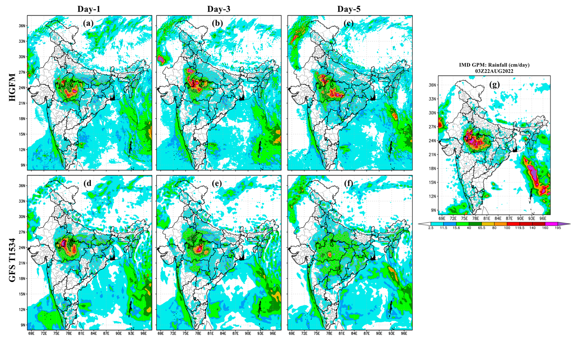
Figure 9 Comparison of the heavy-rainfall event on 22 August 2022 with HGFM (a–c) and GFS T1534 (d–f) for 1 d, 3 d, and 5 d lead times with IMD GPM (g) rainfall.

To attain further clarity about the model precipitation and moist convective processes, the vertical profile of relative humidity as a function of rain rate is analyzed for JJAS of 2022 over the ISM region (10° S–30° N, 60–100° E). The bias analysis suggests that GFS T1534 has systematically underestimated the lower-level moisture for all lead times (Fig. 8b). This is consistent with the findings of Mukhopadhyay et al. (2019) and Ganai et al. (2021), who reported a similar underestimation of lower-level moisture over the ISM region in the GFS T1534 forecast. In contrast, HGFM shows relative improvement in the lower-level moisture distribution, as depicted in Fig. 4c for all lead times. The enhancement of the lower-level moisture is noticeable compared to the GFS T1534 forecast. However, the upper troposphere is too moist in both model forecasts and requires further improvement.

It is observed that the overall statistics of monsoon rainfall and related convective processes have significantly improved in HGFM. In the next section, a case of heavy rainfall is discussed, followed by the analysis of recent tropical cyclone forecasts.

3.5 Evaluation of a heavy-rainfall event

A very heavy-rainfall event occurred on 22 August 2022 over central India. This event was captured well by both GFS T1534 and HGFM compared to the observed rain from IMD-GPM (shown in Fig. 9). Both HGFM (Fig. 9a–c) and GFS T1534 (Fig. 9d–f) simulated the heavy-rainfall signature compared to IMD-GPM (Fig. 9g) in the 1 d and 3 d forecasts. However, a significant difference was noted in rainfall intensity and spatial distribution at longer lead times (5 d) in HGFM and GFS T1534. Both the models underestimated rainfall compared to observations. Nevertheless, HGFM captures the signal of heavy-rainfall occurrence even at a 5 d lead time, which is almost negligible in the GFS T1534 forecast. Further, the precipitation probability distribution function (PDF) is analyzed (figure not shown) for the JJAS 2022 monsoon. It is found that HGFM shows a better PDF in the very heavy (11.56–20.45 cm d⁻¹) and extreme (> 20.45 cm d⁻¹) rainfall categories compared to GFS T1534.

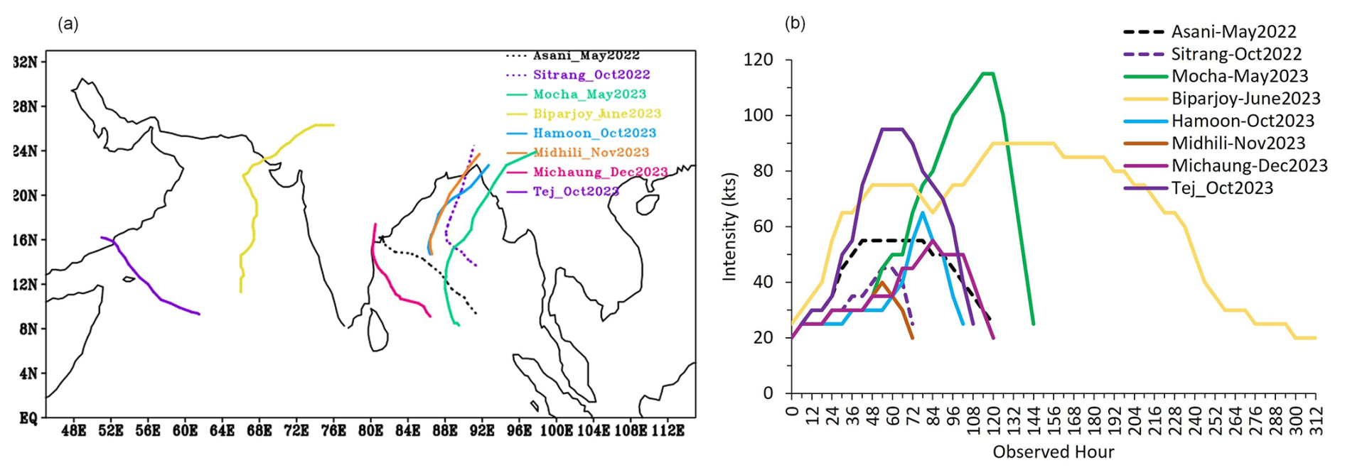
Figure 10 (a) Observed cyclone tracks and (b) observed intensity in terms of maximum sustained wind speed (kn) during the year 2022–2023 (1 kn = 0.514 m s⁻¹).

3.6 Evaluation of tropical cyclone forecasts

A total of eight named tropical cyclones that occurred during 2022 and 2023 (RSMC 2022, RSMC 2023) are considered in the present study. Out of these eight cases, two cyclones formed over the Arabian Sea and six cyclones over the Bay of Bengal (BOB). The best data for the track, intensity, and landfall are obtained from IMD and are referred to as observations henceforth in the text. Figure 10 shows the observed tracks (Fig. 10a) and observed intensity in terms of the maximum sustained wind speed (MSW Fig. 10b) of the cyclones. The cyclones in the present study have different tracks and various ranges of severity in terms of intensity over both basins.

3.6.1 Verification of GFS T1534 and HGFM forecasts for tropical cyclone cases during 2022 and 2023

For this verification, the lifetime of the cyclone is considered from the depression stage until landfall, as per the observations. The total sample includes a minimum of 4 and a maximum of 10 initial conditions for typical cases, depending on the lifespan of the case. The errors calculated here are averaged for each forecast hour within the sample.

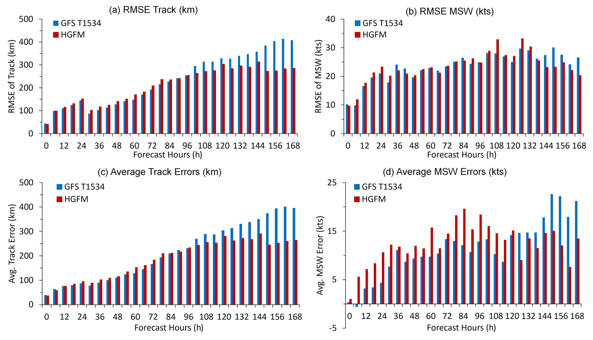
Figure 11 (a) RMSE of the track (km), (b) RMSE of MSW (kn), (c) the average track error (km), and (d) the average intensity errors (kn).

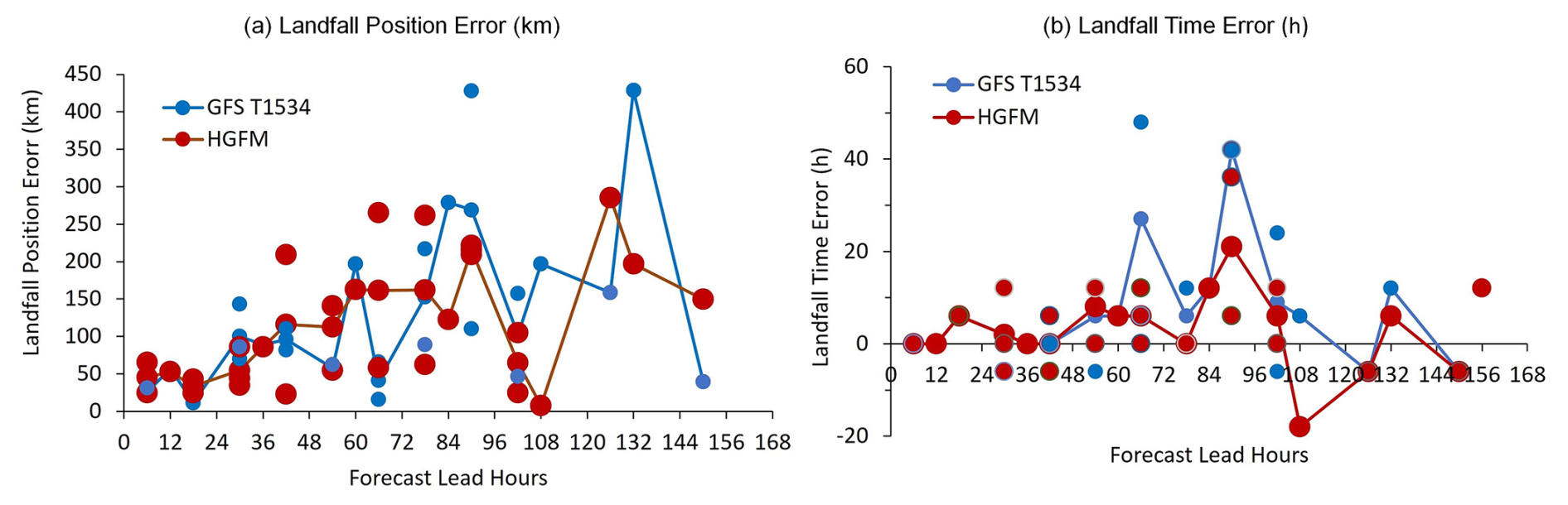
Figure 12 (a) Average landfall position errors (km) and (b) average landfall time errors (h). The continuous lines represent the average errors for GFS T1534 (blue) and HGFM (red). The different sizes of the dots are to make the overlapping points visible.

The root-mean-square errors (RMSEs) for track and intensity are shown in Fig. 11a and b, respectively. Initially, up to day 4, GFS T1534 and HGFM perform equally well, but considerable improvement with HGFM is noted after 4 d in both track and intensity forecasts. Figure 11c and d depict the average track error and average intensity errors for all the cyclones. The average track errors, as well as average intensity errors, are reduced drastically in HGFM with longer lead times (4 d or more). The average track errors (average intensity errors) are ∼ 300 km (∼ 20 kn; 1 kn = 0.514 m s⁻¹) with 7 d leads in HGFM. The average landfall errors (both position and time) are also evaluated with IMD observations and are shown in Fig. 12. With 4 d of lead, average landfall position errors are ∼ 200 km in HGFM and about 250 km for GFS T1534. Overall, the landfall position errors are smaller for HGFM. Remarkable improvements are seen in the average landfall time errors in HGFM throughout the life cycle of the cyclones. Overall, the track and intensity forecast are improved with HGFM for longer lead times (∼ 4 d or more), which is an added advantage for early warning and mitigation purposes. Here, one of the cyclone cases (Cyclone Biparjoy) is discussed in detail.

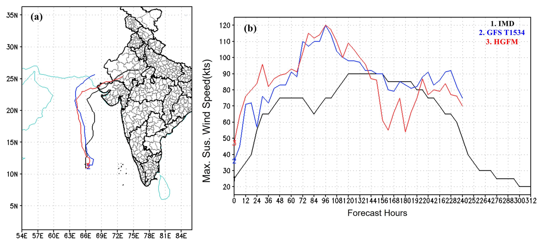
Figure 13 (a) Track and (b) intensity variation forecast by GFS T1534 and HGFM and as reported by IMD for the case of tropical Cyclone Biparjoy over the Arabian Sea, which is based on the 6 June 2023 initial condition.

3.6.2 A case study – Cyclone Biparjoy

During the monsoon onset of the 2023 season, tropical Cyclone Biparjoy evolved in the Arabian Sea and hit the northwestern state of Gujarat, India. Cyclone Biparjoy lasted for quite a long time, 6–19 June 2023. As seen in Fig. 13a, it moved almost parallel to the Indian west coast and eventually recurved to make landfall over the northern part of Gujarat and adjoining Pakistan. It underwent rapid intensification during its genesis and growth stages on 6 and 7 June. This case was particularly challenging for prediction due to the combination of recurving track, rapid intensification, slow movement, and a long lifespan. The HGFM and GFS T1534 track and the intensity forecast of TC (tropical Cyclone) Biparjoy based on the 6 June (the day of genesis) initial condition are shown in Fig. 13a and b, along with the best-track data from IMD. It is evident that HGFM predicts a track much closer to the observations compared to GFS T1534. In particular, the recurvature is better captured by HGFM at about a 6–7 d lead time. Both models overestimated the intensity until 120 h into the forecast, after which they indicated the dissipation phase.

Table 2 Landfall position (km) and landfall time (h) errors for the forecasts started with different initial conditions. The negative (positive) values indicate early (late) landfall with respect to the observed landfall time. The bold numbers indicates significant improvements in the landfall position errors with HGFM.

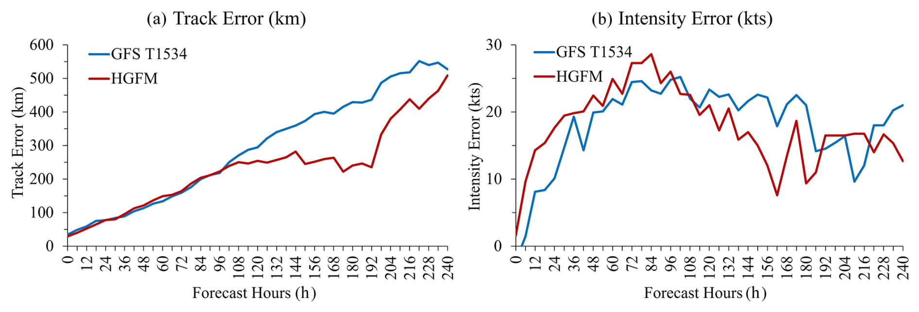
Figure 14 (a) Average track error and (b) average intensity error for tropical Cyclone Biparjoy over the Arabian Sea.

To assess the robustness of the performance, verification is carried out for this particular case, considering forecasts from all the initial conditions (from 6 June 00:00 UTC to 15 June 00:00 UTC, initialized at 24 h intervals). A comparative analysis of the landfall position and landfall time errors for HGFM and GFS T1534, with respect to the data reported by IMD, is presented in Table 2. It is evident that the landfall position error in the cyclone has been significantly improved by the HGFM forecast, although the landfall time error appears to be almost equivalent to GFS T1534. Further, the average track and intensity errors (obtained from a total of 10 initial conditions) are depicted in Fig. 14a and b. It is evident that HGFM consistently produces accurate predictions of track and intensity with smaller errors at longer lead times, while the errors for shorter lead times are more or less the same.

4 Conclusions

For the first time, a version of the GFS model utilizing a new grid structure, the triangular–cubic–octahedral (Tco) grid, has been developed and is being run on an experimental basis for short- to medium-range weather prediction over the Indian region, designated the IITM High-Resolution Global Forecast Model (HGFM). The Tco grid provides a higher resolution over the tropics, enabling the model to achieve a 6.5 km horizontal resolution near the tropics. This higher resolution represents a substantial leap from the existing Gaussian linear GFS T1534, which maintains a resolution of 12.5 km across the globe. The KE spectra of 200 hPa zonal wind have also revealed reasonable power by both the models, with HGFM showing marginally better power in the Kolmogorov region, indicating the fidelity of the model structure.

It is worth mentioning that the present dynamical core, using the cubic–octahedral grid, has been implemented in the ECMWF weather forecast model since 2016 (Malardel et al., 2016). This has led to a significant increase in forecast accuracy and computational efficiency in the ECMWF model. In the present study, it was found that this dynamical core in the GFS T1534 has improved the orographic rainfall and reduced the Gibbs noise over the mountainous regions, in addition to the improved precipitation skill over the Indian landmass region. The June–September monsoon rainfall and a case study of heavy rainfall have been analyzed in detail. The newly developed HGFM shows significantly better skill, particularly with longer lead times and for heavier rain categories. Rainfall biases over the entire globe appear broadly similar in HGFM and GFS T1534. A case of heavy rainfall in and around central India during the monsoon season has been analyzed, where validation shows a significant gain in forecast lead time by HGFM compared to GFS T1534. HGFM captures the rainfall signature at a 5 d lead time, when there is hardly any indication in the GFS T1534 model forecast.

Several cases of tropical cyclones in 2022 and 2023 were analyzed, indicating better performance of HGFM compared to GFS T1534 in predicting tracks and intensity. A detailed evaluation of tropical Cyclone Biparjoy based on IMD observations reveals that HGFM provides better accuracy in cyclone position across almost all lead times (Table 2). Additionally, the average track error for HGFM is significantly lower than GFS T1534 at longer lead times. However, the average track and intensity errors for both the models are found to be equivalent. This paper highlights the initial results of the newly developed HGFM and its skill compared to the operational GFS T1534 model. Subsequently, more analyses for many events will be carried out, and the model will be made operational for weather forecasts over India. The current setup of HGFM uses the same physics as the GFS model. However, HGFM would require some parameter tuning to optimize and enhance the performance of the model and its fidelity. Future work will be focused on detailed validation of model simulations with an optimal set of physical parameterizations.