NSOAS24: a new global marine gravity model derived from multi-satellite sea surface slopes

Judging by the early release of the NSOAS22 model, there were some known issues, such as boundary connection problems in blockwise solutions and a relatively high noise level. By solving these problems, a new global marine gravity model, NSOAS24, is derived based on sea surface slopes (SSSs) from multi-satellite altimetry missions. Firstly, SSSs and along-track deflections of vertical (DOVs) are obtained by retracking, resampling, screening, differentiating, and filtering procedures on the basis of altimeter waveforms and sea surface height measurements. Secondly, DOVs with a ${\mathrm{1}}^{\prime }\times {\mathrm{1}}^{\prime }$ grid interval are further determined using Green's function method, which applies directional gradients to constrain the surface, least-squares fit to constrain noisy points, and tension constraints to smooth the field. Finally, the marine gravity anomaly is recovered from the gridded DOVs according to the Laplace equation. Throughout the entire processing procedure, improvements in accuracy are expected for the NSOAS24 model due to the following changes, e.g., supplementing recent mission observations and removing old mission data, optimizing the step size during Green's function method, and special handling in nearshore areas. These optimizations effectively resolved the known issues of signal aliasing and the “hollow phenomenon” in coastal zones. Typical altimetry-derived marine gravity models are the DTU series released by the Technical University of Denmark and the S&S series released by the Scripps Institution of Oceanography (SIO), University of California San Diego (UCSD). Their latest models, DTU21 and SS V32.1, were used for comparison and validation. Numerical verification was conducted in three experimental areas (the Mariana Trench area, Mid-Atlantic Ridge area, and Antarctic area, representing low-, mid-, and high-latitude zones) with DTU21, SS V32.1, and shipborne data. Taking NSOAS22 for comparison, NSOAS24 showed improvements of 1.2, 0.7, and 1.0 mGal in the three test areas by validating with SS V32.1, while declines of 0.6, 0.5, and 0.3 mGal and 0.2, 0.4, and 0.3 mGal occurred in SD statistics with DTU21 and shipborne data. Finally, NSOAS24 was assessed using two sets of shipborne data (the early National Centers for Environmental Information (NCEI) dataset and the later dataset from the Japan Agency for Marine-Earth Science and Technology (JAMSTEC), the Marine Geoscience Data System (MGDS), the French Oceanographic Cruises Directory (FOCD), and the French Naval Hydrographic and Oceanographic Service (SHOM)) on a global scale. Generally, NSOAS24 (6.33 and 4.95 mGal) showed a comparable accuracy level with DTU21 (6.20 and 4.71 mGal) and SS V32.1 (6.40 and 5.53 mGal) and better accuracy than NSOAS22 (6.64 and 5.64 mGal). The new model is available at https://doi.org/10.5281/zenodo.12730119 (Zhang et al., 2024).

1 Introduction

Satellite altimetry provides highly accurate ocean surface height measurements with respect to certain ellipsoids along corresponding ground tracks (Fu and Cazenave, 2001; Stammer and Cazenave, 2017). Among these altimetry satellites, some have performed geodetic missions (GMs) with longer revisit periods and denser spatial coverage, which provide the primary data sources for marine gravity recovery. Exact-repeat missions (ERMs) are also critical to relevant research according to a relatively lower noise level by averaging nonunique, repetitive cycles (Zhang et al., 2022). Due to new altimetry technology and advanced processing methods, the accuracy of sea surface height (SSH) measurements has increased dramatically over the last decade (Andersen et al., 2023), with a positive influence on marine gravity model constructions. The refinement of altimetry-derived marine gravity models has become more obvious due to these recent altimetry missions with dense spatial coverage since 2010, e.g., CryoSat-2, SARAL/AltiKa, Jason-1, Jason-2, and Haiyang-2A (HY-2A) GM (Chen et al., 2024). Combining observations from multiple satellites with different orbital inclinations, such as 108, 98, 92, and 66°, enables a more reliable determination of the marine gravity field (Andersen and Knudsen, 2019; Sandwell et al., 2021). In addition to conventional nadir altimeters, synchronized laser beams for obtaining reflected surface height information, two-satellite companion mode, and wide-swath altimetry techniques offer new observations and require effective incorporating strategies for modeling the marine gravity field. Furthermore, these advancements provide new opportunities and potential for recovering refined marine gravity anomalies. Generally, combining multi-frequency and multi-mode altimetry data, especially observations with higher range accuracy, denser spatial coverage, and diverse track directions, is an effective way of refining marine gravity recovery (Sandwell et al., 2021).

China launched the Haiyang-2A (HY-2A) satellite in 2011 and initiated its geodetic mission in 2016 for the purpose of geodetic applications. Multiple previous studies have shown that HY-2A has consistent accuracy compared with other conventional altimetry missions (Wan et al., 2020; Zhang et al., 2020; Guo et al., 2022). Moreover, its successors, including HY-2B, HY-2C, and HY-2D, were successively launched in 2018, 2020, and 2021. Although HY-2 data cannot serve as the sole input for constructing a ${\mathrm{1}}^{\prime }\times {\mathrm{1}}^{\prime }$ marine gravity anomaly model (Wan et al., 2020; Zhang et al., 2022), the HY-2 series of measurements are extremely valuable for recovering marine gravity anomalies because of their unique spatial distributions. Currently, several institutions have effectively adopted HY-2 series data to release regional or global marine gravity models, such as SCSGA V1.0 (Zhu et al., 2020), NSOAS22 (Zhang et al., 2022), GMGA1 (Wan et al., 2022), SDUST2021GRA (Zhu et al., 2022), and GMGA2 (Hao et al., 2023). Besides the HY-2 series, the most well-known altimetry-derived marine gravity models are the DTU and S&S series, which are released by the Technical University of Denmark and the Scripps Institution of Oceanography (SIO), University of California San Diego (UCSD), respectively. To some extent, they represent the highest attainable accuracy (Li et al., 2021; Mohamed et al., 2022). Their latest versions have been updated to DTU21 and S&S V32.1.

In a previous study of the released NSOAS22 model, we primarily evaluated the performance of HY-2 series altimeter data in constructing marine gravity fields and highlighted the role played by HY-2. However, we found some obvious issues identified in NSOAS22 through systematic evaluation. First and foremost is the boundary connection problem in blockwise solutions, which leads to a sawtooth-like discontinuity in the final recovered marine gravity signals. Therefore, this paper aims to address existing issues and to optimize the model construction steps for the purpose of constructing a refined marine gravity model. These specific improvements contain dataset filtering and optimization (supplementing recent observations and removing low-quality data), re-designing the step sizes to solve DOVs with Green's functions, and special processing in nearshore areas. These improvements are further described in detail in Sect. 4.

The remainder of this paper is organized as follows. Section 2 provides a general description of the included datasets (altimeter data and shipborne data), as well as the reference gravity models used for comparison and the remove–restore procedure. The theoretical methods for DOV calculation and gravity anomaly inversion are presented in Sect. 3. Section 5 evaluates the altimetry-derived global marine gravity model using the well-known altimetry-derived models and shipborne measurements. Finally, conclusions are given in Sect. 6, focusing on the ${\mathrm{1}}^{\prime }\times {\mathrm{1}}^{\prime }$ global marine gravity anomaly model named NSOAS24.

2 Research data

2.1 Altimetry data

The newly accumulated altimetry data have provided not only high-quality SSH observations but also diverse spatial distributions. For these recent missions, we selected sensor geophysical data records (SGDRs), which include high-sampling waveforms from the Jason-1, Jason-2, Jason-3, CryoSat-2, HY-2A, HY-2B, and SARAL/AltiKa satellites. In addition, Jason-1, Jason-2, and SARAL/AltiKa adopt both ERM and GM data, HY-2A uses only GM data, and HY-2B and Jason-3 use only ERM data. CryoSat-2 data comprise three modes: a low-resolution mode (LRM), synthetic aperture radar (SAR), and synthetic aperture radar interference (SIN). Taking into account the previously collected dataset, Geosat observations from both GM and ERM with a unique 108° orbital inclination angle, along with ERS-1 GM, Envisat ERM, and TOPEX/Poseidon ERM datasets, were also utilized. Envisat acquired ERM data for two repeated periods, 30 and 35 d. Detailed information on the included altimetry data is listed in Table 1.

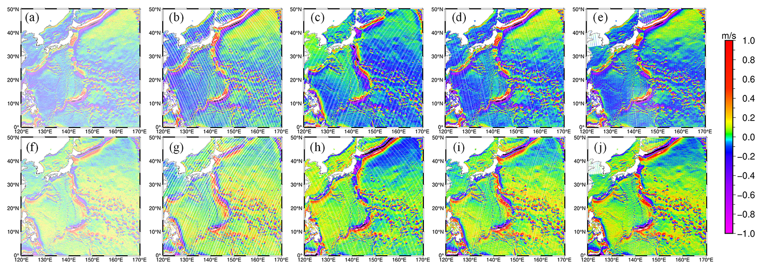
Figure 1 Slope plot of satellite ascent and descent at different orbital inclinations ((a)–(e) represent ascending track slopes for HY-2A (99.3°), Geosat (108°), Jason-2 (66°), SARAL/AltiKa (98.55°), and CryoSat-2 (92°), respectively; (f)–(j) represent descending track slopes for HY-2A, Geosat, Jason-2, SARAL/AltiKa, CryoSat-2, and respectively).

Table 1 Information on altimetry satellites used for deriving the gravity field.

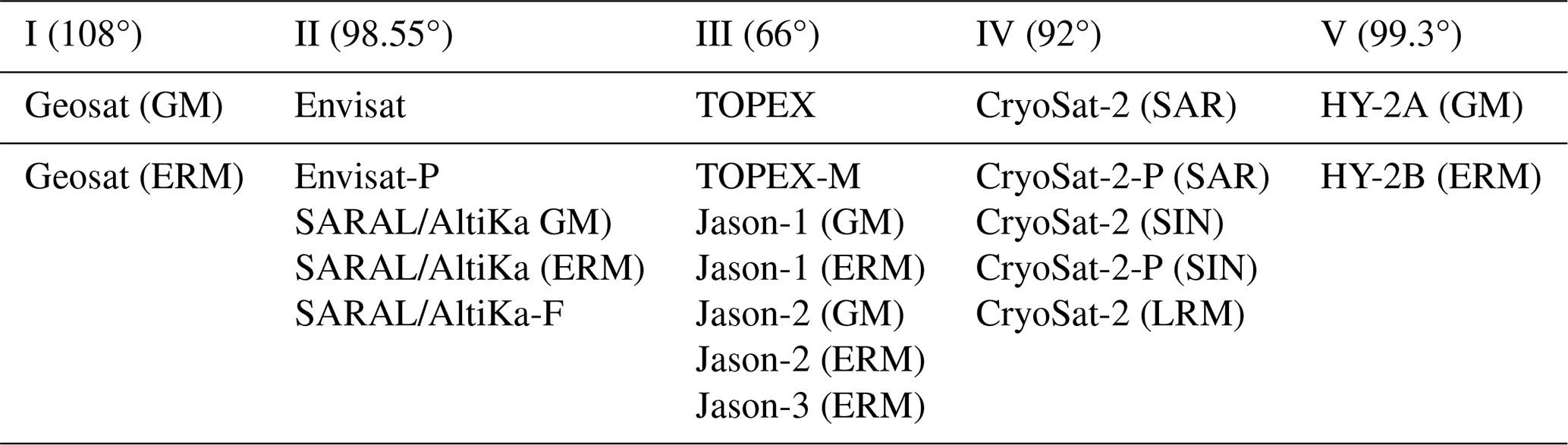
Along-track SSSs can be regarded as vector data, and their magnitude is determined by the time interval between adjacent ground track points and corresponding SSH variations. Due to different designs of satellite orbital inclinations and ground track orientations (ascending or descending), along-track SSSs capture different signal variations and similar signal variation magnitudes with opposite signs. As shown in Fig. 1, satellites with different orbital inclinations exhibit significant differences in along-track slopes obtained in the Mariana Trench area. Ascending and descending orbit data both reflect the overall regional trend, exhibiting horizontal symmetry in direction and being numerically nearly opposite. For instance, the orbital inclination of HY-2A is approximately 99°, allowing it to obtain actual data reaching up to around 81° in high-latitude regions. In contrast, other altimetry satellites are limited by their designed orbital parameters, such as the Jason series, which cannot measure data beyond the 66° region. Satellites with near-polar orbit have a data coverage advantage in high-latitude regions. Considering the spatial coverage and orientations, the calculated slopes should be stored separately based on different orbital inclinations and directions to ensure consistency. Consequently, we categorized these satellites in Table 1 into five groups based on their orbital design, as shown in Table 2. For multi-cycle data, these are appended to the same data file without disrupting temporal continuity, in preparation for subsequent segment-based slope editing steps.

Table 2 Grouping of satellites according to different orbital inclinations.

2.2 Typical gravity models

To compare and validate the new global marine gravity model, several well-known models are introduced. Firstly, the latest version of the S&S series model, which includes both DOV and gravity anomaly, is used for comparison and validation purposes, hereinafter referred to as V32.1. Secondly, the DTU21 gravity anomaly model is introduced for comparison and validation. Thirdly, the classical EGM2008 comprehensive series model is introduced, which provides the SSH along with the DOT2008A mean dynamic topography model, DOV, and gravity anomaly (Pavlis et al., 2012). It serves as the reference model in the remove–restore procedure.

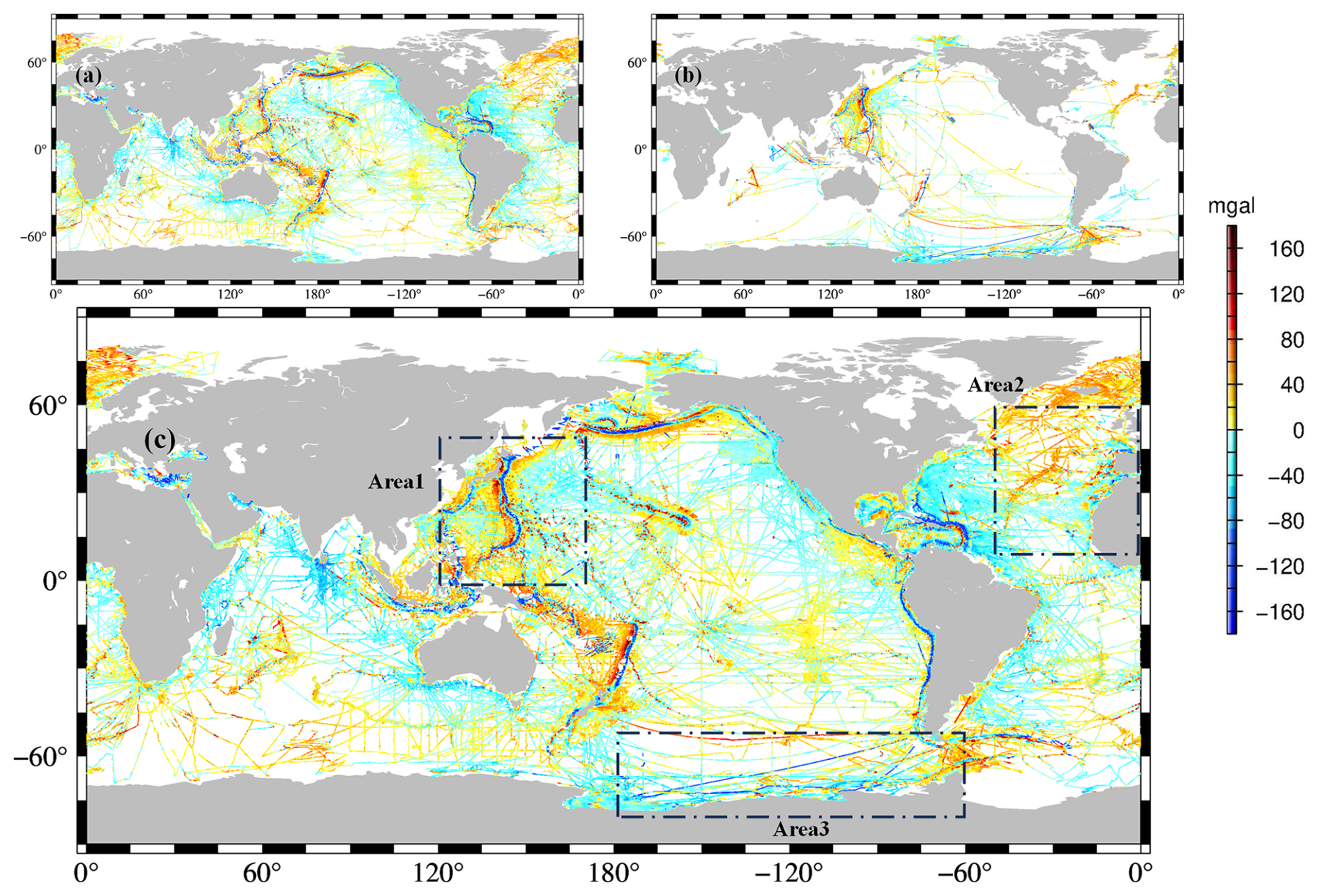
Figure 2 Distribution of shipborne data ((a) NCEI; (b) FOCD, JAMSTEC, MGDS, SHOM; (c) total shipborne data, with the three experimental areas highlighted with dashed rectangles).

2.3 Shipborne data

Firstly, a total of 10 740 231 old shipborne data points were collected from the National Centers for Environmental Information (NCEI). Secondly, a total of 33 522 351 recent measurements from four marine institutions with relatively high quality were gathered: the French Oceanographic Cruises Directory (FOCD), the Japan Agency for Marine-Earth Science and Technology (JAMSTEC), the Marine Geoscience Data System (MGDS), and the French Naval Hydrographic and Oceanographic Service (SHOM). The distribution of shipborne data is illustrated in Fig. 2. The NCEI data cover global oceans more comprehensively, whereas non-NCEI data exhibit dense coverage in the nearby regions of Japan and in the partial Antarctic seas. Due to inevitable outliers in in situ data, necessary data editing was conducted using the triple-standard-deviation criterion by calculating deviations with respect to the EGM2008 model. As shown in Fig. 2c, three regions, which are marked in dashed rectangles and span low-, mid-, and high-latitude oceans (area 1: 0–50° N, 120–170° W; area 2: 10–60° N, 310–360° W; area 3: 50–80° S, 180–300° W), were selected as experimental areas.

3 Theoretical methodology

3.1 Method of along-track DOV calculation

Instead of the derivative of the geoid with respect to the spherical distance, Sandwell and Smith (1997) proposed a method of calculating along-track DOV with two steps. Firstly, geoid slopes were derived from adjacent geoid heights and corresponding temporal variations. Secondly, the along-track DOV is computed on the basis of geoid slopes by dividing by the corresponding velocity derived by the satellite orbit parameter. The procedure is summarized in the following formula.

$$\begin{array}{}\text{(1)}& {\mathit{\epsilon }}^{\mathit{\alpha }}=-{\displaystyle \frac{\partial N}{\partial s}}=-{\displaystyle \frac{\partial N}{\partial t}}\cdot {\displaystyle \frac{\partial t}{\partial s}}=-{\displaystyle \frac{\partial N}{\partial t}}\cdot {\displaystyle \frac{\mathrm{1}}{v}}\end{array}$$

Here, N is the height of the geoid, s is the spherical distance, and t is the observation time. The process for determining the linear velocity v is as follows. Given a data point's latitude φ, we first convert the geodetic latitude to the geocentric latitude φ_c by considering the Earth's flattening e. The formula is expressed as follows:

$$\begin{array}{}\text{(2)}& {\mathit{\phi }}_{\mathrm{c}}={\displaystyle \frac{\mathrm{1}-e}{\sqrt{{\cos }^{\mathrm{2}}\mathit{\phi }+(\mathrm{1}-e{)}^{\mathrm{4}}{\sin }^{\mathrm{2}}\mathit{\phi }}}}.\end{array}$$

Assuming the inclination angle of the satellite's orbit is α, the period of the orbit's descending node is T, the regression period is t, the distance between adjacent trajectories is s, and the equatorial circumference is L, the average angular velocity w_s and synchronous Earth velocity w_e of the satellite's elliptical motion along the orbit can be calculated separately:

$$\begin{array}{}\text{(3)}& {\displaystyle }& {\displaystyle }{w}_{\mathrm{s}}={\displaystyle \frac{\mathrm{2}\mathit{\pi }}{T}},\text{(4)}& {\displaystyle }& {\displaystyle }{w}_{\mathrm{e}}={\displaystyle \frac{w_{\mathrm{s}}tL}{s}}.\end{array}$$

Subsequently, the angular velocity components w_φ and w_λ along the latitude and longitude directions can be obtained separately:

$$\begin{array}{}\text{(5)}& {\displaystyle }& {\displaystyle }{w}_{\mathit{\phi }}={\displaystyle \frac{w_{\mathrm{s}}{\cos }^{\mathrm{2}}\mathit{\phi }}{(\mathrm{1}-e{)}^{\mathrm{2}}{\cos }^{\mathrm{2}}{\mathit{\phi }}_{\mathrm{c}}}}\sqrt{\mathrm{1}-{\displaystyle \frac{{\cos }^{\mathrm{2}}\mathit{\alpha }}{{\cos }^{\mathrm{2}}{\mathit{\phi }}_{\mathrm{c}}}}},\text{(6)}& {\displaystyle }& {\displaystyle }{w}_{\mathit{\lambda }}={\displaystyle \frac{w_{\mathrm{s}}\cos \mathit{\phi }}{{\cos }^{\mathrm{2}}{\mathit{\phi }}_{\mathrm{c}}}}-w_{\mathrm{e}}.\end{array}$$

We can obtain the angular velocity w along the orbit with a simple synthesis:

$$\begin{array}{}\text{(7)}& w=\sqrt{w_{\mathit{\phi }}^{\mathrm{2}}+w_{\mathit{\lambda }}^{\mathrm{2}}}.\end{array}$$

Finally, we multiply by the radius of the Earth R to obtain the ground linear velocity v:

$$\begin{array}{}\text{(8)}& v=wR.\end{array}$$

3.2 Method of gridded DOV calculation

Green's method proposed by Wessel and Bercovici (1988) restores the along-track DOV to the gradient direction of the geoid and subsequently projects it onto the prime (east–west) and meridional (north–south) components, achieving a similar transformation in the along-track components (Brammer and Sailor, 1980). For a linear operator L, the output or response under the action of a point source δ is Green's function G,

$$\begin{array}{}\text{(9)}& LG=\mathit{\delta },\end{array}$$

where L is taken as the Laplace operator ∇²,

$$\begin{array}{}\text{(10)}& \mathrm{\nabla }=i{\displaystyle \frac{\partial }{\partial x}}+j{\displaystyle \frac{\partial }{\partial y}}+k{\displaystyle \frac{\partial }{\partial z}}.\end{array}$$

Green's function formulation transforms into

$$\begin{array}{}\text{(11)}& {\mathrm{\nabla }}^{\mathrm{2}}\mathit{\varphi }\left(x\right)=\mathit{\delta }\left(x\right).\end{array}$$

The left-hand side of the above equation represents the product of the Laplace operator and Green's function formulation, while the right-hand side corresponds to the Dirac delta function. Solutions that satisfy the Laplace equation are known as harmonic functions, corresponding to cases where the divergence is zero. The formulation for biharmonic functions is introduced as follows:

$$\begin{array}{}\text{(12)}& {\mathrm{\nabla }}^{\mathrm{4}}\mathit{\varphi }\left(x\right)=\mathit{\delta }\left(x\right).\end{array}$$

Spline interpolation, whether in one or two dimensions, corresponds physically to enforcing a thin elastic beam or plate to conform to data constraints. The same interpolation principles apply to Green's two-dimensional function formulation as follows:

$$\begin{array}{}\text{(13)}& D{\mathrm{\nabla }}^{\mathrm{4}}\mathit{\varphi }\left(x\right)-T{\mathrm{\nabla }}^{\mathrm{2}}\mathit{\varphi }\left(x\right)=\mathit{\delta }\left(x\right).\end{array}$$

In the equation, D represents stiffness, and T denotes the tension factor.

In the discrete case, the following equation holds when there are M reference points within the region:

$$\begin{array}{}\text{(14)}& D{\mathrm{\nabla }}^{\mathrm{4}}w\left(x\right)-T{\mathrm{\nabla }}^{\mathrm{2}}w\left(x\right)=\sum _{j=\mathrm{1}}^M{c}_j\mathit{\delta }\left(x-x_j\right).\end{array}$$

Wessel and Bercovici (1988) derived the solution w(x) through Fourier transformation as

$$\begin{array}{}\text{(15)}& {\displaystyle }& {\displaystyle }w\left(x\right)=\sum _{j=\mathrm{1}}^M{c}_j\mathit{\varphi }\left(x-x_j\right),\text{(16)}& {\displaystyle }& {\displaystyle }\mathit{\varphi }\left(x\right)=K_{\mathrm{0}}\left(p\left|x\right|\right)+\log \left(p\mathrm{|}x\mathrm{|}\right).\end{array}$$

When there are N known points within the region, the following equation matrix can be constructed:

$$\begin{array}{}\text{(17)}& w_i=\sum _{j=\mathrm{1}}^M{c}_j\mathit{\varphi }\left(x_i-x_j\right)i=\mathrm{1},N.\end{array}$$

Thus,

$$\begin{array}{}\text{(18)}& w=Gc.\end{array}$$

The along-track DOV is the projection of the gradient of the geoid along the track direction. The inverse solution is obtained using Green's function method, simultaneously applying tension spline functions to ensure curve smoothness. The fundamental concept is to simulate the geoid field using a finite number of control points. This approach aims to interpolate and recover the DOV at all grid points. In discrete conditions, Green's method formula is shown as Eq. (14), where the left-hand side represents selected control points, and the right-hand side consists of other known points with radial basis functions. By iteratively solving from the known points towards the control points, the radial basis coefficients c_j are determined. This process can be viewed as constructing the geoid field ϕ using finite elements.

Considering that ϕ(x) and w_i are scalar fields representing the geoid and their corresponding geoid heights, the actual input data represent the directional derivatives of the geoid, specifically the along-track DOV vector information. Therefore, introducing the gradient field gradϕ(x) is formulated as follows in Eq. (19):

$$\begin{array}{}\text{(19)}& {\displaystyle }& {\displaystyle }\mathrm{\nabla }\mathit{\varphi }\left(x\right)=i{\displaystyle \frac{\partial \mathit{\varphi }}{\partial x}}+j{\displaystyle \frac{\partial \mathit{\varphi }}{\partial y}}+k{\displaystyle \frac{\partial \mathit{\varphi }}{\partial z}},\text{(20)}& {\displaystyle }& {\displaystyle }{\mathit{s}}_i=(\mathrm{\nabla }w\cdot n{)}_i=\sum _{j=\mathrm{1}}^M{c}_j\mathrm{\nabla }\mathit{\varphi }\left(x_i-x_j\right)\cdot n_{i}i=\mathrm{1},N,\text{(21)}& {\displaystyle }& {\displaystyle }D=\sum _{j=\mathrm{1}}^M{c}_j\mathrm{\nabla }\mathit{\varphi }\left(x_i-x_j\right)i=\mathrm{1},N.\end{array}$$

When simultaneously taking the directional derivative in the satellite operation direction n_i on both sides, s_i represents the along-track DOV vector. ∇ϕ(x) corresponds to the gradient field of the geoid. Considering the varying quality of data from different satellites, uncertainties “sig” are incrementally added to control data quality. Therefore, an equation matrix can be constructed at reference points:

$$\begin{array}{}\text{(22)}& \begin{array}{rl}& \left[\begin{array}{l}{s}_{\mathrm{1}}/{\mathrm{sig}}_{\mathrm{1}}\\ \mathrm{⋮}\\ s_n/{\mathrm{sig}}_n\end{array}\right]={\left[\begin{array}{l}{c}_{\mathrm{1}}\\ \mathrm{⋮}\\ c_m\end{array}\right]}^T\\ & {\left(\begin{array}{lll}\mathrm{0}& \mathrm{\cdots }& D_{x_{\mathrm{1}}-x_m}{n}_{\mathrm{1}}/{\mathrm{sig}}_{\mathrm{1}}\\ \mathrm{⋮}& \mathrm{\ddots }& \mathrm{⋮}\\ D_{x_n-x_{\mathrm{1}}}{n}_n/{\mathrm{sig}}_n& \mathrm{\cdots }& \mathrm{0}\end{array}\right)}^T\\ & i=\mathrm{1},Nj=\mathrm{1},M.\end{array}\end{array}$$

After solving for the coefficients c_j, the construction of the geoid gradient field is completed. At any grid point, the geoid gradient D can be determined. Multiplying this gradient by the east–west and north–south directional vectors yields the DOV components at each grid point.

Green's function method offers several advantages. Firstly, it innovatively applies directional gradients rather than SSH to constrain the model surface in order to enhance stability. Secondly, it employs least-squares fitting instead of exact interpolation, effectively mitigating the impact of noisy data points. Additionally, by incorporating tension constraints, it facilitates data smoothing. For moderate data volumes, Green's function method is superior to traditional finite-difference methods. However, Green's functions also present certain limitations, such as their inability to handle excessively large datasets, challenges with boundary discontinuities, and suboptimal performance in nearshore areas. These issues are discussed and addressed in Sect. 4.

3.3 Method of deriving gravity anomalies

The relationship between DOV and gravity disturbances or anomalies can be deduced by the Laplace equation (Sandwell and Smith, 1997). The relationships are established according to the internal connections among the disturbing potential T, gravity disturbances δg, gravity anomaly Δg, and two directional components of DOV (ξ and η). Assuming a flat-Earth approximation, the disturbing potential T satisfies the Laplace equation in the given local planar coordinate system (x, y, z). Then, the relationship between gravity and DOV can be established as the following equation.

$$\begin{array}{}\text{(23)}& {\displaystyle \frac{\partial \mathit{\delta }g}{\partial z}}=-{\mathrm{{\rm Y}}}_{\mathrm{0}}\left({\displaystyle \frac{\partial \mathit{\xi }}{\partial x}}+{\displaystyle \frac{\partial \mathit{\eta }}{\partial y}}\right)\end{array}$$

Taking the difference between the gravity disturbance and gravity anomaly into account, the gravity anomaly is further calculated according to

$$\begin{array}{}\text{(24)}& \mathrm{\Delta }g\left(xy\right)=\mathit{\delta }g\left(xy\right)-{\displaystyle \frac{\mathrm{2}{\mathrm{{\rm Y}}}_{\mathrm{0}}}{R}}N\left(xy\right),\end{array}$$

where R is the average radius of Earth, and N is the geoid height, which can be provided by geopotential models. For a detailed computation procedure, refer to Zhang et al. (2020).

4 Model construction

Based on the theories summarized in Sect. 3, we sequentially calculated along-track SSH, SSS, along-track DOV, gridded DOV, and gridded gravity anomalies from multi-frequency and multi-mode satellite altimetry data. For the purpose of model construction, a series of joint processing strategies, e.g., waveform retracking, adding corrections, resampling, data editing, filtering, and the remove-and-restore procedure, were necessary. The specific construction steps are illustrated in Fig. 3.

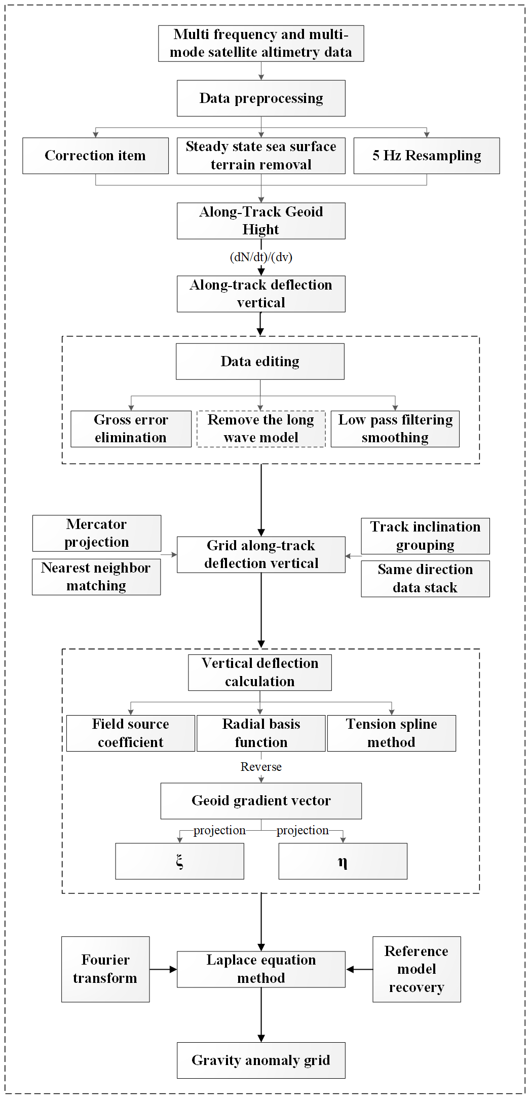
Figure 3 Flowchart of constructing the marine gravity model from multi-satellite altimeter data.

4.1 Data preprocessing and slope editing

Firstly, raw waveforms were retracked using the two-step weighted least-squares retracker (Zhang and Sandwell, 2017), and high-rate observations along profiles were uniformly resampled into 5 Hz to constrain the noise level and enhance the density of available measurements. Secondly, along-track SSH measurements were calculated by adding correction items provided in the sensor data record (SDR) products to amend corresponding effects for path delay and the geophysical environment. The along-track slopes were then calculated, and their accuracy was validated with the EGM2008 model slopes. If the deviations exceed the setting threshold according to the triple-standard-deviation criterion, the data point is considered unreliable and removed. If excessive data segments are edited out, the entire segment is abandoned to prevent the influence of outliers on subsequent calculations. Finally, a Parks–McClellan filter was applied to all slopes to constrain the amplified high-frequency noise during the difference procedure. Marine gravity models derived from conventional nadir altimeters achieve an accuracy of approximately 2–3 mGal and require low-pass filtering at wavelengths of at least 14 km to suppress short-wavelength noise (Sandwell et al., 2021). Based on this standard, we used a Parks–McClellan filter with a cutoff wavelength of 16 km.

4.2 Gridding along-track DOV

Firstly, along-track velocities corresponding to different satellites were calculated to convert along-track slopes to along-track DOVs. Along-track residual DOVs were then computed by filtering the EGM2008 geoid heights and corresponding DOT2008A_n180 mean dynamic topography. Before gridding, it is necessary to define the objective grid in advance. Considering that the inversion grid should closely resemble the real Earth, a Mercator projection grid was chosen in this study. The Mercator projection is a cylindrical map projection that preserves angles and is used for a ${\mathrm{1}}^{\prime }\times {\mathrm{1}}^{\prime }$ global grid, with 21 600 grid points in both latitude and longitude directions. (The latitude direction uses the Gudermannian function transformation, while the longitude direction is uniformly divided.) After defining the gridding points, along-track slopes were gridded using a nearest-neighbor approach. Satellites are categorized based on orbital inclination and ground track orientation, which ensures that the along-track DOV direction remains consistent and averages potentially redundant data points in the same direction at grid points, thereby reducing data complexity. Due to the requirements of Green's function method regarding region size and data volume, the convergence of multiple vectors with different values at the same gridding points but with consistent directions can lead to matrix singularity. It is worth mentioning that the averaging step between each category was essential to address this issue.

As mentioned above, along-track DOVs were mapped to gridding points. Taking the HY-2 group for instance, the gridding process for ascending and descending track segments is illustrated in Fig. 4. Matching is performed using the nearest-neighbor method, and data stacking follows the principle of consolidating data in the same direction. The specific process is summarized as follows. (1) Determine the number and position of the ${\mathrm{1}}^{\prime }\times {\mathrm{1}}^{\prime }$ grid points implemented using the Mercator projection. (2) Project the geodetic latitude and longitude of input data onto Mercator coordinates, and determine the nearest grid point in the Mercator coordinate system for each data point. (3) Perform weighted averaging for data in the same direction, and store data from different groups separately.

Figure 4 Gridding along-track DOVs at grid points (HY-2 group for example).

4.3 DOV component calculation

Limited by the computing power of computer and massive gridding points, the DOV components were calculated with blockwise input and output to avoid excessive computational redundancy and matrix singularity. While constructing the NSOAS22 model, the tension spline method overlooked the impact of coherence between blockwise regions. This tension spline interpolation is typically suitable for solving small- to moderate-sized regions with medium data volumes. However, excessive data can drastically reduce computational efficiency and potentially cause stack overflow issues. Consequently, constraints arising from the distribution of known points may lead to ineffective solving at boundaries and discontinuities between adjacent regions, as illustrated in Fig. 5a. In this study, we proposed a new solution by enlarging computation regions while restricting output to central areas to ensure continuity. Specifically, the inputs were chosen within a 64×64 grid, and the outputs were exclusively limited to the central 32×32 grid. As illustrated in Fig. 5b, the discontinuous effect was eliminated.

Figure 5 Result of spline splicing method for DOV east–west components ((a) original; (b) new).

Figure 6 Green's function method for solving DOV components.

4.3.1 Step selection

To compute DOV components using Green's function method, it is necessary to select specific grids as control points for iterative processes. A graphical representation of solving DOV components using Green's function method is illustrated in Fig. 6. Additionally, the tension spline interpolation demonstrates optimal performance when control points are evenly distributed. Leveraging the regularity of the grid, the step size (interval between two control points) is defined for selecting control points. An increased number of control points tends to render the spline curve more rigid, thereby accentuating large fluctuations and noise. Conversely, a reduced number of control points leads to a sparser spline curve that appears smoother, effectively mitigating noise. However, sparse control points may result in an overly simplistic representation of the field. As control points become sparser, the interpolation distance increases, thereby reducing the reliability of the results.

Our computational grid size is 64×64, offering different control point densities based on step sizes: 4096 control points with a step size of 1, 1024 with a step size of 2, and 441 with a step size of 3. Larger step sizes lead to fewer control points, which may not adequately represent the region. Step size 1 results in excessive noise, affecting signal continuity and computational efficiency. Hence, step sizes 2 and 3 are under consideration in our study to balance detail and computational feasibility.

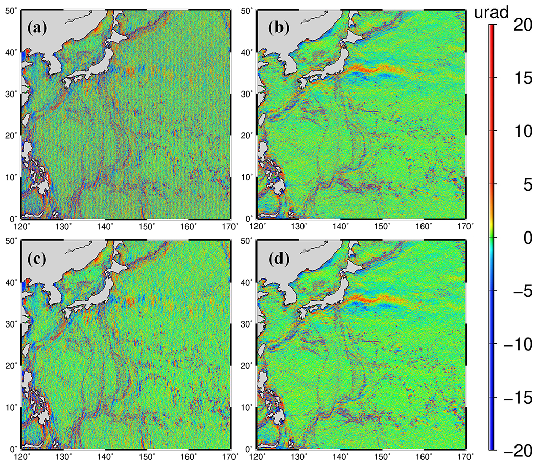
Figure 7 Residual results of DOV component differences for different step size selections ((a) east–west component at two steps, (b) north–south component at two steps, (c) east–west component at three steps, (d) north–south component at three steps).

In experimental area 1 in Fig. 2c, the residual DOV for step sizes 2 and 3 is shown in Fig. 7. The figure demonstrates that with a step size of 2, noticeable noise artifacts are introduced, particularly impacting the east–west components. In contrast, using a step size of 3 results in smoother outcomes, exhibiting clearer distribution characteristics of the DOV components. The reduction in noise is particularly effective in specific areas like nearshore regions and islands.

We then analyzed the distribution of noise under different step sizes. V32.1 serves as a verification model, against which the DOV results obtained with a step size of 2 are subtracted. The standard deviation is 3.19 µrad for the east–west component and 2.02 µrad for the north–south component. Setting a threshold based on the triple-standard-deviation criterion, the primary noise locations are depicted in Fig. 8a and b. There are 125 456 noise points in the east–west component, accounting for 1.20 % of the entire region, and 122 976 noise points in the north–south component, making up 1.19 % of the total area. After removing these noise points, the standard deviations reduce to 2.45 µrad for the east–west component and 1.36 µrad for the north–south component. With a step size of 3, the standard deviations are 2.37 µrad for the east–west component and 1.75 µrad for the north–south component. Identified based on the triple-standard-deviation criterion, the primary noise locations are shown in Fig. 8c and d. There are 77 904 noise points in the east–west component, accounting for 0.75 % of the entire region, and 105 923 noise points in the north–south component, comprising 1.02 % of the total area. After removing outliers, the standard deviations decrease to 1.84 µrad for the east–west component and 1.20 µrad for the north–south component.

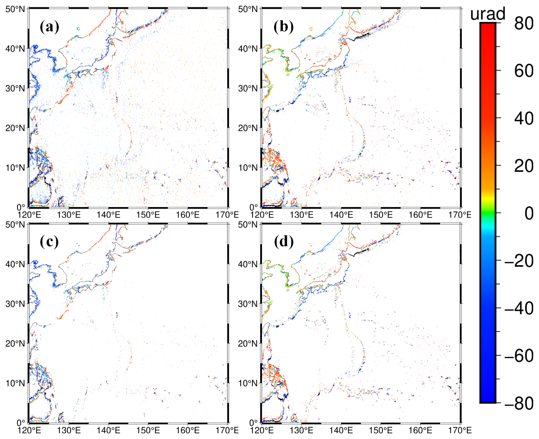
Figure 8 Noise analysis at different step sizes ((a) east–west component at step size 2, (b) north–south component at step size 2, (c) east–west component at step size 3, (d) north–south component at step size 3).

The noise histogram with different step sizes, as shown in Fig. 9, provides a more intuitive demonstration that a step size of 3 effectively reduces noise compared to a step size of 2. Notably, the east–west component exhibits a noticeable reduction in noise when using a step size of 3. Moreover, scattered noise points in open ocean areas are massively eliminated. This is to say, the selection of step size significantly influences both the distribution and the magnitude of noise points. Considering larger step sizes' advantages in enhanced computational efficiency, reduced matrix complexity, and lower mitigation noise, we finally selected step size 3 for acquiring controlling points.

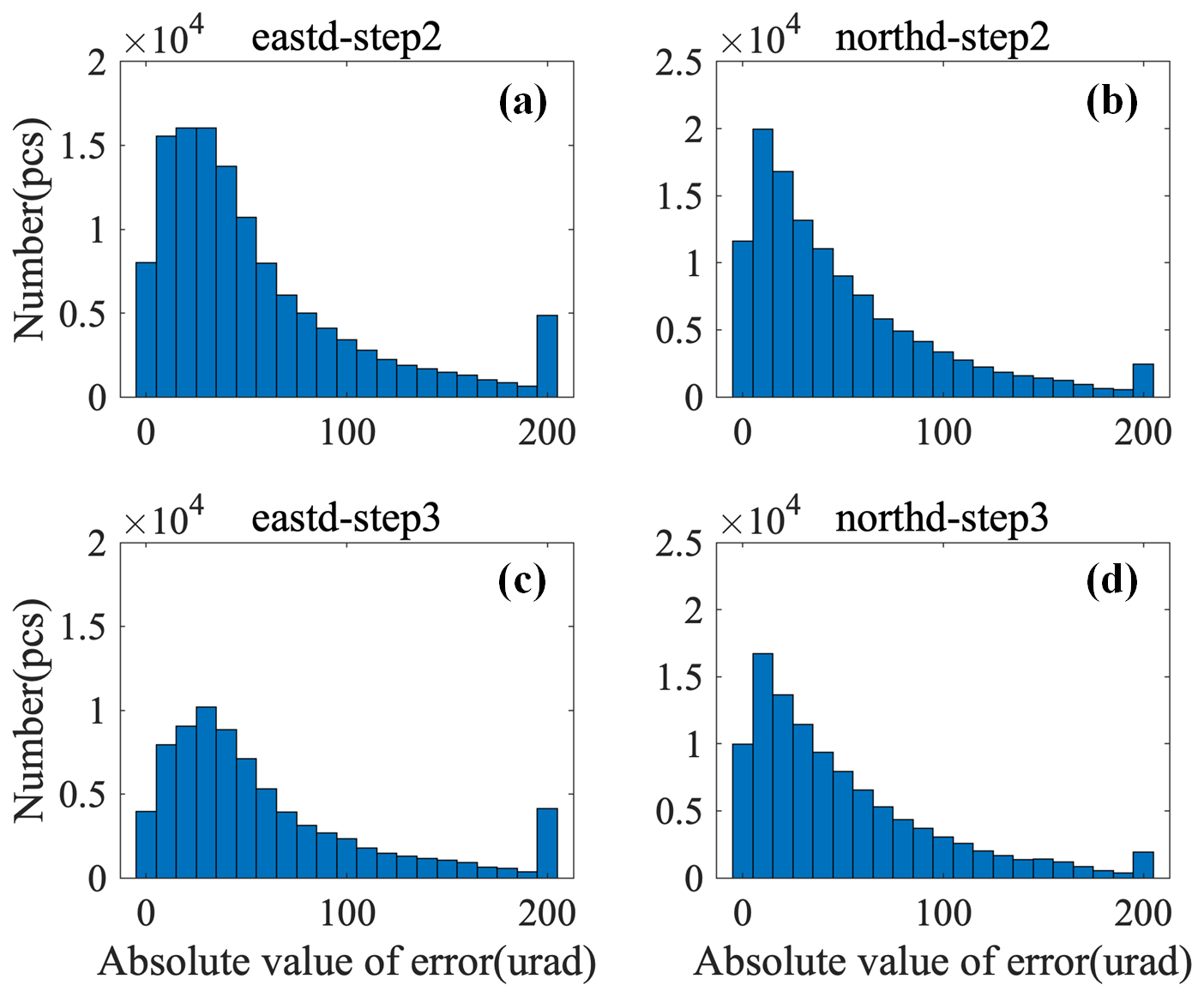
Figure 9 Noise histogram with different step sizes ((a) east–west component at step size 2, (b) north–south component at step size 2, (c) east–west component at step size 3, (d) north–south component at step size 3).

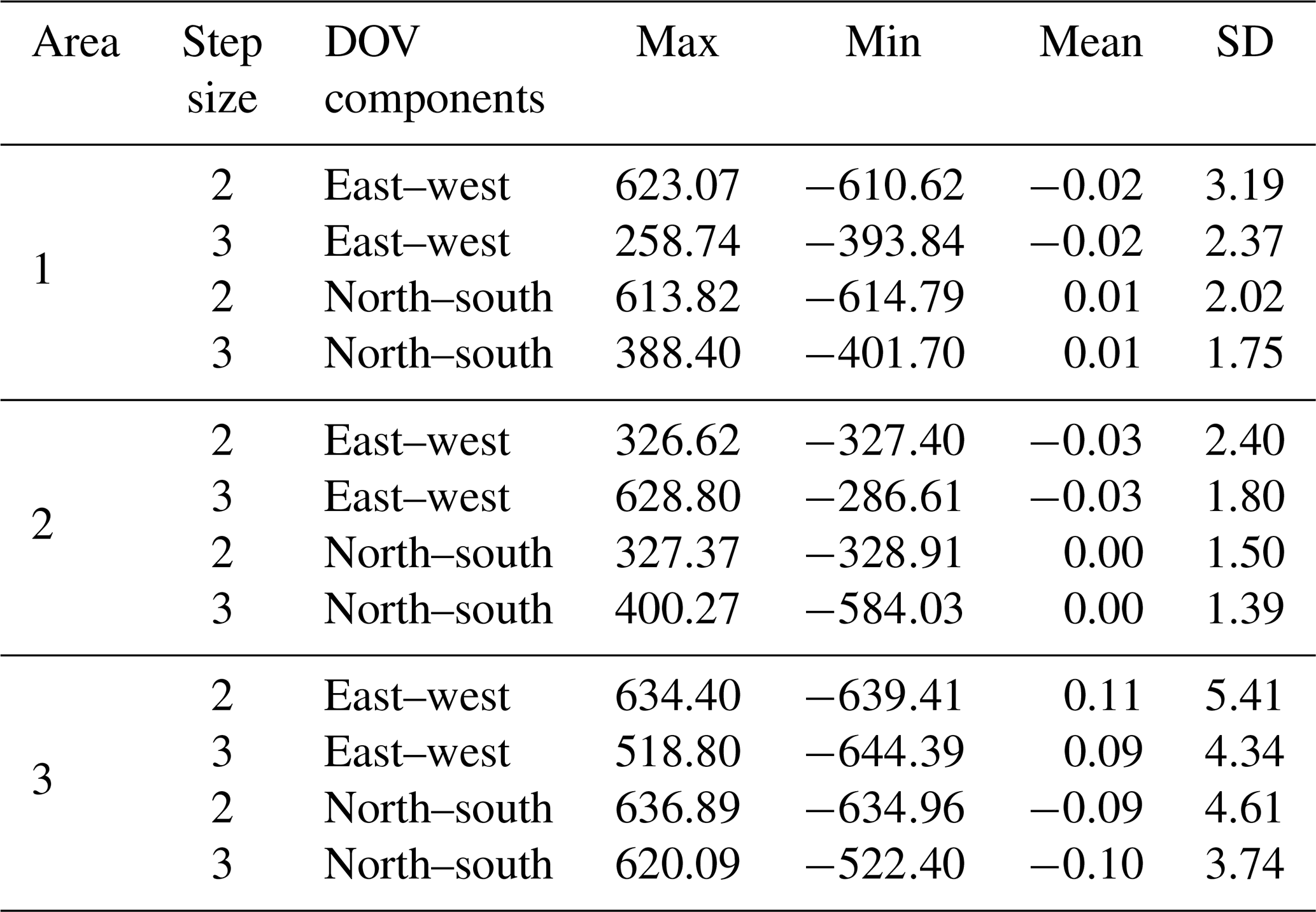
In addition, comparisons between step sizes were conducted in two other experimental areas, and the statistical results are presented in Table 3. It is interesting that experimental area 3 exhibits distinctive characteristics. Satellites with lower inclinations, such as the TOPEX/Poseidon and Jason series, are unable to provide observations beyond 66°, and area 3, a region with high ocean dynamics in the Southern Ocean, exhibits a noticeable decline in DOV quality in high-latitude regions.

Table 3 Statistics of DOV components with respect to V32.1 for different step sizes (unit: µrad).

4.3.2 Special processing in nearshore areas

Along the coastline, SSH measurements are typically available only on the ocean side, while grid points over land are default values and pose computational challenges. As illustrated in Fig. 8, increasing the step size effectively reduced a considerable number of noise points over the open sea, while the remaining noise points majorly concentrated in nearshore areas. To demonstrate the effect of special processing in nearshore areas, we chose the sea around China and its adjacent waters (0–40° N, 100–140° E) as the experimental area. This area is densely distributed with islands and reefs, involving typical categories of coastal regions. Based on the calculated residual DOV with respect to V32.1, we distinguished noise points where the absolute deviation exceeds 20 µrad. The distribution of noise points near the coastlines is more pronounced, as shown in Fig. 10. The east–west component and north–south component noise points account for 0.27 % and 0.09 % of the total grid points in the region, respectively. It is evident that larger noise points are more prevalent in the anomalous computation of the east–west component. Therefore, special treatment is required in nearshore areas to mitigate the concentrated occurrence of noise. As previously mentioned, Green's function method operates within a 64×64 grid area. When handling nearshore regions, the grids over land lack data, with controlling points only available on the ocean side. Thus, the actual data boundary is at the coastline but not at the edges of the 64×64 grid. These mixed zones directly cause boundary effects that hinder matrix convergence. Expanding the computation area is not a feasible solution because even with an enlarged area, there are no effective data points over land to provide constraints. Solutions without constraints typically exhibit lower reliability, contributing significantly to the observed noise in coastal areas. Figure 11 further gives these differences between the calculation and V32.1 over land-influenced 64×64 grid areas, showing the approximate outline of the blockwise rectangular computational regions in finer detail. The influential grid points in nearshore areas account for 10 % of the total grid points. Additionally, 30 % of grid points over land are within the influential region, indicating a significant proportion of nearshore grid points.

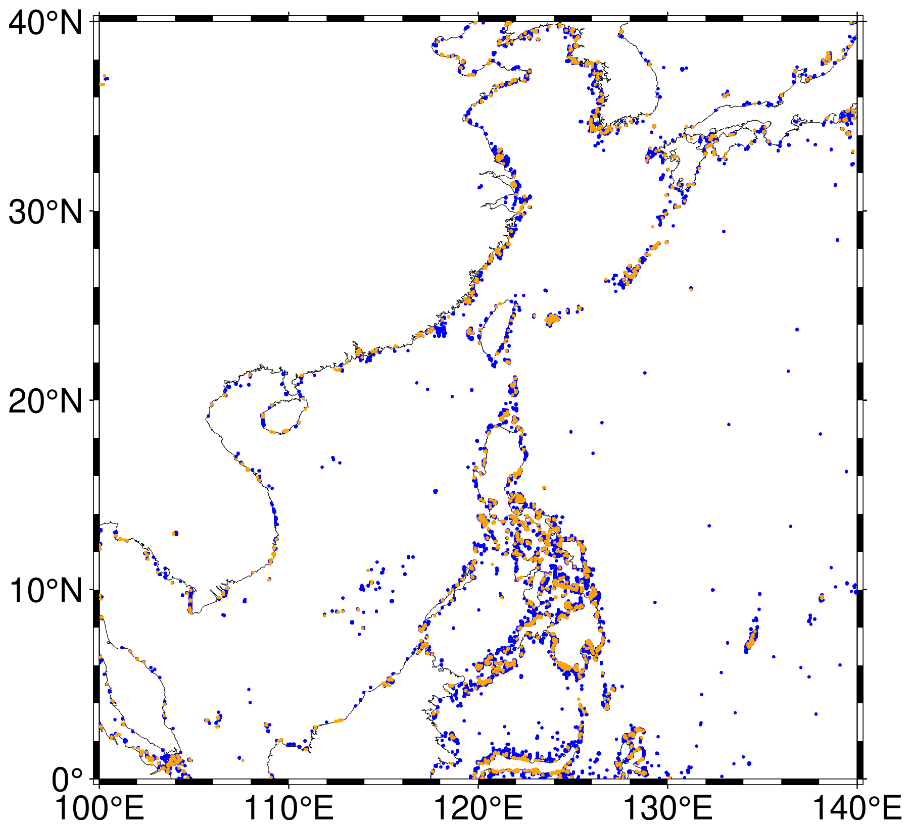
Figure 10 The main locations of noise distribution in the nearshore area (east–west component in orange; north–south component in blue).

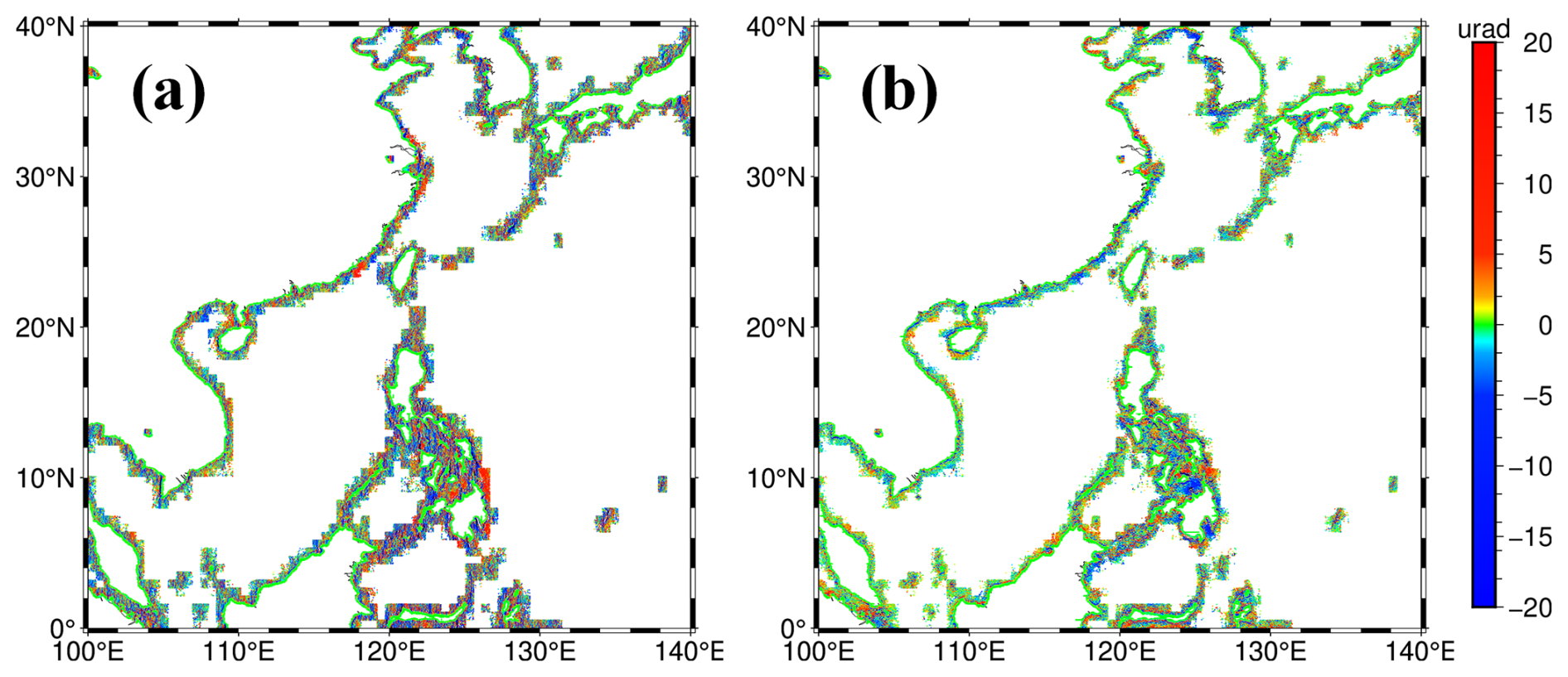
Figure 11 Location of distribution of nearshore areas disturbed by continental regions ((a) east–west component; (b) north–south component).

To constrain this boundary effect, special processing steps were implemented. A continental mask was applied to identify controlling points over land, which were assigned a value of 0 and treated as known points. Moreover, these points were assigned relatively huge uncertainties to minimize their weight. This approach effectively mitigated boundary effects, thereby controlling data divergence and improving the reliability of computations in these land-influenced regions. Figure 12 illustrates the difference in nearshore points before and after processing. Following the adjustments, there is almost no change on the seaward side, while on the landward side, the standard deviation shows a difference of 1.67 µrad in the east–west component and 1.47 µrad in the north–south component, with a maximum difference of around 60 µrad. This indicates that this special processing effectively suppressed the occurrence of large noise points near the coastlines.

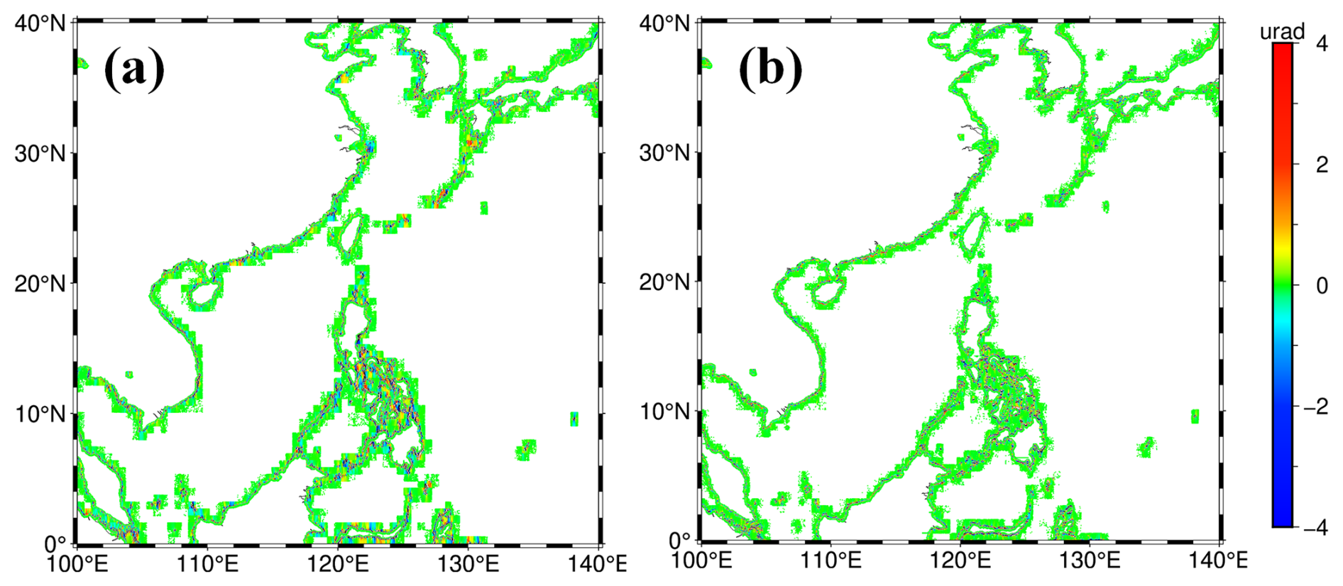
Figure 12 Difference in results in the nearshore area before and after the special processing ((a) east–west component; (b) north–south component).

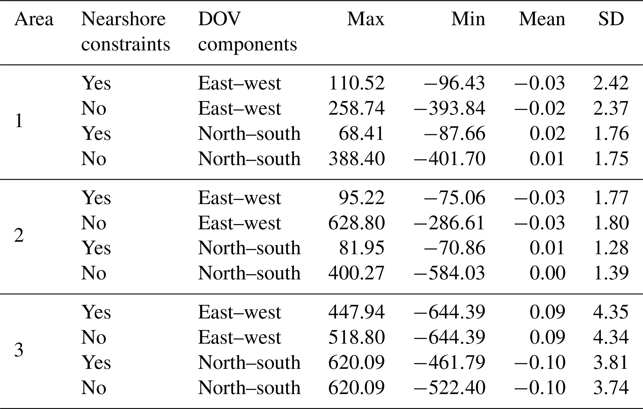
Statistical analysis was also conducted in the three experimental areas, and the results are listed in Table 4. First and foremost is that the nearshore constraint effectively reduced the magnitude of maximum and minimum deviations. In areas 1 and 2 in particular, maximum and minimum values declined notably, indicating an effective constraint on the occurrence of large noise spikes. Moreover, similarly using a deviation threshold of 20 µrad for identifying noise points decreased the overall noise ratios by 17.6 % following this optimization effort.

Table 4 Statistics on the difference with respect to V32.1 with or without nearshore constraints (unit: µrad).

4.3.3 Remove ERS-1 data

To evaluate the contribution of each individual mission to multi-satellite altimetry-derived DOV, each satellite (SARAL/AltiKa, Envisat, HY-2A and HY-2B, Geosat, and ERS-1) was sequentially removed within the sea around China and its adjacent waters (0–40° N, 100–140° E). Median absolute deviations (MADs) of the east–west and north–south components along latitude were computed, with the NSOAS24 DOV without data removal used as a comparison. Land-influenced zero values were excluded during this experiment. The results are presented in Fig. 13, which illustrates that SARAL/AltiKa provides the most reliable data and the largest contribution. HY-2 also significantly influences the DOV, resulting in discrepancies exceeding 2.5 µrad in the east–west component and ranging from 1 to 1.5 µrad in the north–south component. ERS-1 and Geosat have a relatively minor contribution, causing differences of less than 1.5 and 1 µrad in the east–west and north–south components, respectively. This also suggests that their signals overlap to a greater extent with other satellites.

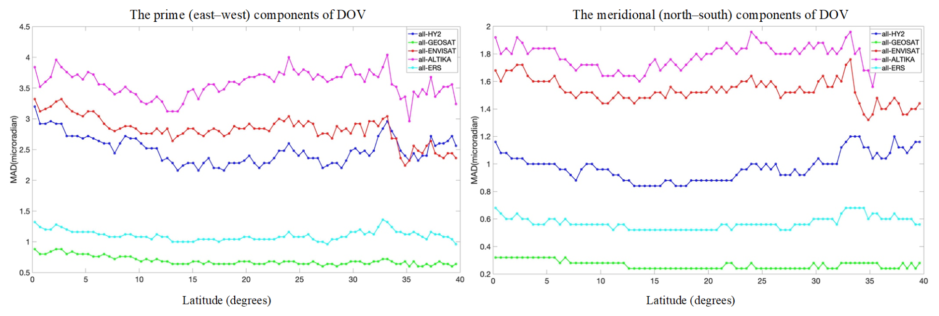
Figure 13 Difference in median absolute deviations between NSOAS24 DOV and DOV in the absence of certain missions (the greater the difference, the larger the influence).

Additionally, DOV components were calculated for several single satellite missions, and the MAD between them and V32.1 in the latitude direction was compared. As shown in Fig. 14, the MAD values are consistently small for HY-2, Envisat, and SARAL/AltiKa. However, the data from Geosat and ERS-1 exhibit significant deviations, suggesting considerably higher noise levels.

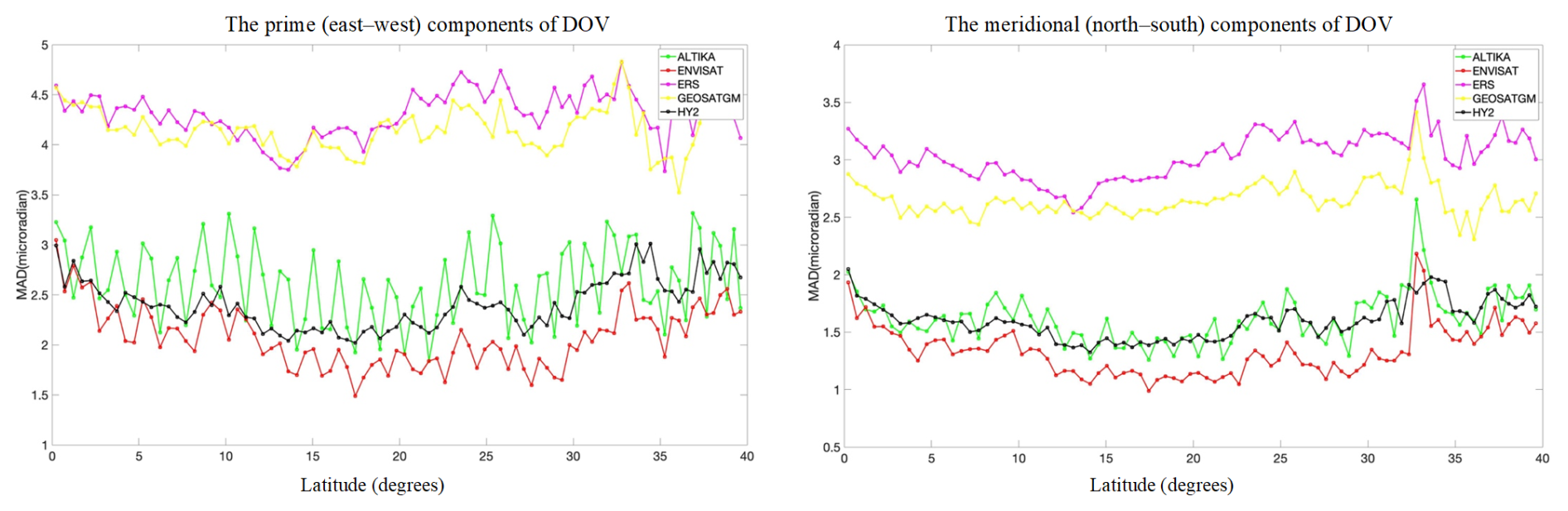
Figure 14 Difference in median absolute deviations between V32.1 DOV and the single satellite solution (the smaller the difference, the better the DOV solution).

Due to being in the early stages of satellite altimetry, Geosat and ERS-1 may suffer from inherent ranging errors and orbit determination issues that could lead to degraded data quality. Considering the vast number of observations accumulated in recent decades, it is worthwhile to consider removing low-quality and redundant data. For Geosat, its extensive accumulated data volume and dense coverage in high-latitude regions, coupled with its unique 108° orbital inclination, make it a distinct group of observations with an independent direction. Therefore, we have chosen to temporarily retain Geosat data in the NSOAS24 model construction. ERS-1 has also accumulated a significant amount of data. However, within the same directional group in Table 2, SARAL/AltiKa and Envisat share a substantial number of grid points that overlap completely with ERS-1 (accounting for 30.7 % of overlap). During the gridding process, these overlapping data points were stacked. In other words, 30.7 % of ERS-1's data can be entirely replaced by higher-precision data from SARAL/AltiKa and Envisat. From the perspective of controlling points, it is noteworthy that control points in all directions exhibit a duplication rate exceeding 95 %. Therefore, with adequate data coverage, multidirectional and high-quality precise slope data are required. Considering the previously identified poor performance and high replaceability, ERS-1 data have ultimately been removed from the NSOAS24 model construction.

4.4 Gravity anomaly inversion procedure

Based on the DOV components at grid points, the residual gravity anomalies were calculated using the fast Fourier transform (FFT) method according to the Laplace-equation-derived relationship, and the results are shown in Fig. 15. Finally, a global marine gravity model over a range of 80° S–80° N with a ${\mathrm{1}}^{\prime }\times {\mathrm{1}}^{\prime }$ grid interval, named NSOAS24, was constructed after restoring the removed reference model, as shown in Fig. 16.

Figure 15 The residual gravity anomaly map of NSOAS24.

Figure 16 The gravity anomaly map of NSOAS24.

5 Gravity anomaly results

5.1 Comparison with V32.1 and DTU21

Firstly, the reliability of NSOAS24 was validated using altimetry-derived models, e.g., DTU21 and V32.1, with statistical results summarized in Table 5. In area 1 with relatively complex seafloor terrains, which include the Mariana Trench, seamount chains, and numerous nearshore areas, NSOAS24 shows improvements of 0.6 and 1.2 mGal over its predecessor (NSOAS22) compared to DTU21 and V32.1, respectively. In area 2, a predominantly open sea region, NSOAS24 demonstrates enhancements of 0.5 and 0.7 mGal over NSOAS22 compared to DTU21 and V32.1, respectively. Area 3 shows a 0.3 mGal improvement for NSOAS24 over NSOAS22 compared to DTU21 and a 1.0 mGal improvement compared to V32.1.

Table 5 Statistics of NSOAS24 and its predecessor against DTU21 and V32.1 (unit: mGal).

5.2 Comparison with shipborne gravity data

The distribution of shipborne data and corresponding gravity anomalies of the NSOAS24 model in the three experimental areas are illustrated in Fig. 17. In area 1, NCEI data show a relatively even distribution, while JAMSTEC data are concentrated near Japan with dense nearshore coverage. In area 2, NCEI data are involved within the entire region, while FOCD and SHOM data are primarily concentrated along the Mid-Atlantic Ridge. In area 3, NCEI data are sparse, with fewer observations, whereas MGDS data are more evenly distributed and voluminous. Statistical comparisons are presented in Table 6. The analysis highlights that NSOAS24 significantly improves accuracy compared to NSOAS22. Furthermore, NSOAS24 demonstrates accuracy comparable to DTU21 and V32.1 and outperforms V32.1 in the high-latitude polar regions.

Figure 17 Distribution of NCEI and non-NCEI shipborne data and recovered gravity anomalies.

Table 6 Statistics on differences between altimeter-derived models and shipborne gravity data (unit: mGal).

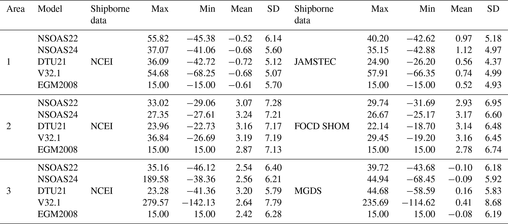
Table 7 Verifications with globally distributed shipborne data (unit: mGal).

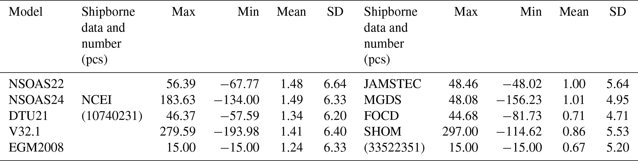
Finally, these models were validated using worldwide-distributed shipborne data. The accuracy of each model was assessed using two sets of shipborne data: the early NCEI dataset and the recent high-quality dataset from JAMSTEC, MGDS, FOCD, and SHOM. The results are summarized in Table 7. In general, NSOAS24 demonstrates accuracy comparable to DTU21 and V32.1. Compared to its predecessor, NSOAS24 shows a steady improvement in accuracy, with a reduction of ∼0.7 mGal in standard deviations when compared with recent non-NCEI shipborne data.

6 Conclusions

Based on our global marine gravity model construction experience in NSOAS22, we initially optimized the dataset by incorporating recent observations and excluding highly substitutable ERS-1 data. Then, multi-satellite datasets were uniformly prepared for constructing a new global marine gravity model. During the processing, satellites with different orbital inclinations were first grouped into five categories. For multi-cycle ERM data, they were appended to the same data file in a way that preserves the temporal continuity of the data without disruption. Secondly, raw waveforms were retracked using the two-step weighted least-squares retracker, and high-rate observations along profiles were uniformly resampled into 5 Hz to enhance the density of available measurements. Thirdly, preprocessing and slope editing were applied to the SSH measurement data to remove outliers, and the Parks–McClellan filter was used to constrain the amplified high-frequency noise during the differencing procedure. Fourthly, the residual along-track DOV was calculated from slopes by dividing by corresponding along-track velocities and introducing EGM2008 as a reference model. Fifthly, gridded DOVs were determined from along-track DOVs by Green's function method. Finally, a global marine gravity model was constructed after FFT and corresponding inverse transform, restoring the removed reference model.

Compared with its predecessor, NSOAS22, several optimizations and improvements were implemented during the entire processing procedure for building NSOAS24. (1) Employing block-based input and output, calculations were executed with a 64×64 grid input, and output was limited to a central 32×32 grid. This improvement effectively resolved poor-accuracy issues at boundaries and eliminated discontinuities between adjacent regions. (2) Utilizing Green's function method to solve the DOV components, we increased the step size from 2 to 3 for selecting grid points as control points for iteration. This optimization aimed to enhance computational efficiency, reduce matrix complexity, and achieve noise smoothing effects. (3) We implemented specialized processing in coastal regions by incorporating a continental mask. The identified land points were assigned a default value with huge uncertainty to mitigate their weight. This approach effectively suppressed boundary effects near coastlines and controlled data divergence.

The new NSOAS24 model was first validated with well-known altimetry-derived models. Comparisons were made in three experimental areas (low-latitude: Mariana Trench area, mid-latitude: Mid-Atlantic Ridge area, high-latitude: Antarctic area) against the DTU21 and V32.1. Compared to its predecessor, NSOAS22, NSOAS24 showed improvements of 0.6, 0.5, and 0.3 and 1.2, 0.7, and 1.0 mGal. Next, we utilized two sets of shipborne data to verify the new model: the earlier NCEI dataset and the recent non-NCEI dataset collected from JAMSTEC, MGDS, FOCD, and SHOM. NSOAS24 also demonstrated a steady improvement in accuracy compared to NSOAS22. Finally, on a global scale, we validated NSOAS24 (6.33 and 4.95 mGal) using the NCEI dataset and the combined dataset from JAMSTEC, MGDS, FOCD, and SHOM (6.20 and 4.71 mGal for DTU21; 6.40 and 5.53 mGal for V32.1). NSOAS24's accuracy was comparable to DTU21 and V32.1, with a notable improvement over NSOAS22 (6.64 and 5.64 mGal). It is worth mentioning that NSOAS24 showed a decline in standard deviations of around 0.7 mGal compared to NSOAS22 when comparing with non-NCEI data. In conclusion, validations with both altimetry-derived models and shipborne data proved the effectiveness of optimizations and the reliability of the NSOAS24 model.