CARIB12: a regional Community Earth System Model/Modular Ocean Model 6 configuration of the Caribbean Sea

A new Community Earth System Model/Modular Ocean Model 6 (CESM/MOM6) ocean-only regional $\mathrm{1}/\mathrm{12}\mathit{°}$ configuration of the Caribbean Sea is presented and validated. The model configuration was developed as a response to the rising need for high-resolution models for climate impact applications. The configuration is validated for the period covering 2000–2020 against ocean reanalysis and a suite of observation-based datasets. Particular emphasis is paid to the configuration's ability to represent the dynamical regime and properties of the region across sub-seasonal, seasonal, and inter-annual timescales. Near-surface fields of temperature, salinity, and sea surface height are well represented. In particular, the seasonal cycle of sea surface salinity and the spatial pattern of the low salinity associated with the Amazon and Orinoco river plumes is well captured. Surface speeds compare favorably against reanalysis and show that the mean flows within the Caribbean Sea (CS) are well represented. The model reproduces known pathways and timing for river plume waters intruding the region. The seasonal cycle of the mixed-layer depth is also well represented, with biases of <3 m when comparing to ocean reanalysis. The vertical structure and stratification across the water column is represented favorably against ship-based observations, with the largest simulated biases in the near-surface water mass and the sub-surface salinity maximum associated with the sub-tropical underwater mass. The temperature and salinity variability in the vertical structure is well represented in the model solution. We show that mean ocean mass transport across the multiple passages in the eastern Caribbean Sea compares favorably to observation-based estimates, but the model exhibits smaller variability and underestimates the mean Yucatán Channel transport when compared to observations and ocean reanalysis estimates. Furthermore, a brief comparison against a 1° CESM global ocean configuration shows that the higher-resolution regional model better represents the extent and seasonality of the Amazon River plume and hence better represents near-surface salinity and mixed-layer depth in the CS. Overall, the regional model reproduces the processes within the Caribbean Sea to a good degree and opens the possibility of regional ocean climate studies in support of decision-making within CESM.

1 Introduction

The Caribbean Sea (CS) is a crucial pathway for ocean circulation. Understanding the dynamics of the Caribbean Sea holds profound implications for global climate patterns (Schmidt et al., 2004; Restrepo et al., 2019; Gradone et al., 2023; Torres et al., 2023) and regional marine biodiversity (Miloslavich et al., 2010; Bowen et al., 2013; Chollett et al., 2012). The inflow to the eastern CS is dominated by two sources, namely (a) North Atlantic waters and (b) tropical Atlantic waters modulated by the large freshwater runoff from the Amazon and Orinoco rivers (Johns et al., 2002; Coles et al., 2013; Hormann et al., 2015; Grodsky et al., 2015; Gradone et al., 2023; Seijo-Ellis et al., 2023). The transport of waters into the eastern CS (from here on referred to as inflow) via the passages along the Greater and Lesser Antilles exhibits variability across different timescales. At the daily to monthly timescales, the near-surface transport may be driven by surface winds (Johns et al., 2002; Andrade-Amaya, 2000) and/or particular river plume events (Seijo-Ellis et al., 2023). The interactions between topography (along the islands in the eastern CS) and density fronts of plume waters result in baroclinic instabilities that often develop into mesoscale eddies that transverse the CS (Andrade and Barton, 2000; Southwick et al., 2016). At the seasonal scale, the near-surface transport and salinity of the CS are dominated by the runoff from the Amazon and Orinoco river plumes peaking in boreal spring and reaching its minimum in early fall (Corredor and Morell, 2001; Johns et al., 2002; Jouanno et al., 2012; Seijo-Ellis et al., 2023). At inter-annual to longer timescales, the flow and properties of the waters entering the eastern CS may be modulated by large-scale modes of variability such as the El Niño–Southern Oscillation and the Atlantic Meridional Mode via coupled processes between the atmosphere, land, and ocean (Restrepo et al., 2014; Arias et al., 2015; Restrepo et al., 2019). Below 100–150 m, the inflow is modulated at inter-annual and longer timescales and is an important component of the Atlantic Meridional Overturning Circulation (AMOC) return flow (Wilson and Johns, 1997; Johns et al., 1999, 2002). The transport includes water masses such as Sargasso Sea Water, Sub-tropical Underwater, Antarctic Intermediate Water, South Atlantic Water, and North Atlantic Deep Water (Corredor and Morell, 2001; Johns et al., 2002; Seijo-Ellis et al., 2019; Gradone et al., 2023). Recent studies suggest that the deep transport of South Atlantic Water through the Anegada Passage may be larger than originally estimated (Gradone et al., 2023). These studies indicate that the inflow of water to the Caribbean Sea is an important component towards understanding changes to the AMOC under a changing climate (Bryden et al., 2005; Frajka-Williams et al., 2019; Caesar et al., 2018).

The Amazon and Orinoco river plumes are also responsible for variability within the Caribbean Current via the generation of vertical shear (Chérubin and Richardson, 2007) that accelerates its mean flow. In addition, the strong near-surface stratification due to the plumes limits vertical mixing and can have important implications for the formation and evolution of tropical storms in the CS by modulating heat fluxes and exchanges with the atmosphere (Godfrey and Lindstrom, 1989; Lukas and Lindstrom, 1991; Rudzin et al., 2017). While the inflow modulates temperature and salinity variability in the CS, there are other important local processes that contribute to upper-ocean variability in the basin. For example, tides across the CS drive local vertical mixing and enhance primary productivity (Kjerfve, 1981; Giese et al., 1990; Sosa, 2001; Ezer et al., 2011) in different areas within the CS. Alongshore winds drive upwelling along the southern CS via Ekman transport (Andrade-Amaya, 2000; Digna et al., 2018), and mesoscale eddies can lead to the formation of thermohaline staircases and mixing via double diffusion (Morell et al., 2006).

Studying these processes for the present day is a relatively straightforward endeavor combining observations and regional ocean models, but at climate scales, additional challenges may arise (Ezer et al., 2011; Solano et al., 2018; Mukherjee et al., 2023; Seijo-Ellis et al., 2023). Coupled climate models have been able to reproduce past and present trends in the Earth system, thus becoming a powerful tool to examine mechanisms and future changes (Hurrell et al., 2013; Meehl et al., 2014; Kay et al., 2015). Nevertheless, the low spatial resolution does not allow us to resolve processes at fine scales, and the dependency on model parameters results in uncertainties across models and against observations (Tebaldi and Knutti, 2007; Hourdin et al., 2017). For example, the typical horizontal resolution for the ocean component in coupled climate models is of 0.25° or coarser, which does not resolve the numerous passages in the eastern CS or the processes that are so intrinsically connected to the topography and geography of the region. Furthermore, certain long-standing biases in climate simulations can often be traced to the ocean component of the coupled model because important oceanic processes are unresolved (or poorly represented), resulting in biases in ocean heat fluxes, air–sea fluxes, and gradients along temperature and density fronts (Large and Danabasoglu, 2006; Kirtman et al., 2012; Danabasoglu et al., 2014; Roberts et al., 2016). More recently, Richards et al. (2021) showed that changes in the mixed-layer depth and buoyancy fluxes under climate change may result in reduced sub-mesoscale activity which, even in the presence of appropriate parameter tuning, may be an additional source of bias in the ocean for climate projections. While there is a rising need for regional climate research to inform decision-making, the shortcomings of global climate models make them unsuited for these purposes. Thus, dynamically downscaling ocean climate projections using a high-resolution ocean model is an enticing proposition to properly examine regional ocean impacts under a changing climate (Chamberlain et al., 2012; Brickman et al., 2021; Richards et al., 2021).

The Community Earth System Model 2 (CESM; Danabasoglu et al., 2020) uses the Parallel Ocean Program (POP2) as its ocean component. However, the Modular Ocean Model 6 (MOM6; Adcroft et al., 2019) is set to replace POP in future versions of CESM. Meanwhile, MOM6 has been made available to users in release versions 2.2 and higher of CESM2. MOM6 uses innovative approaches that make it an ideal model for high-resolution configurations at the regional and global levels. For example, using the arbitrary Lagrangian–Eulerian (ALE) method allows for the use of several different vertical coordinate systems (geopotential, isopycnal, terrain-following, or hybrid), making the model adaptable to the specific constraints of the topography of a region and adaptable to the purposes of the configuration. The model can be run in fully coupled global configurations within CESM, as well as in ocean-only and other supported combinations. In addition, it provides the user with the ability to dynamically downscale the ocean component in global simulations while remaining within the CESM framework. As a first step towards this goal, here we present an ocean-only CESM/MOM6 configuration of the Caribbean Sea. This configuration (hereafter referred to as CARIB12) was developed to understand present and future variability in the near-surface Caribbean Sea waters. This paper focuses on the configuration of the model and a thorough validation for the present-day period (2000–2020) as a benchmark for upcoming future climate projections. In Sect. 2, we describe the model configuration in detail and the datasets and methods used to validate the model. The validation and results are shown in Sect. 3, and conclusions are presented in Sect. 4.

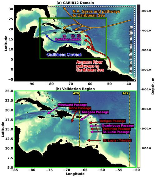
Figure 1 Model domain and topography. (a) CARIB12 regional domain and dominant processes regulating water properties in the Caribbean Sea. The northwestward flow of the Amazon River plume towards the Caribbean Sea is known to branch off in the three main pathways shown (red arrows). The plume waters can affect the vertical structure and strength of the Caribbean Current (blue arrow). Interactions of the flow with the topography along the numerous passages at the Atlantic/Caribbean Sea interface generate mesoscale eddies (magenta) that entrain and transport waters westward. The North Atlantic Gyre dominates the near-surface inflow between the Greater Antilles (orange). The deep flows there form an important return branch of the AMOC. Dashed white lines show the radius of influence of boundary-nudging layers in the configuration. The green box outlines the focus region for the analysis. (b) Validation and analysis region. Arrows indicate the mean flow direction across the multiple passages in the eastern Caribbean Sea and between the Greater Antilles. Dashed yellow lines show the approximate location of WOCE lines A20 and A22 used in the validation.

2 Data and methods

2.1 Model description

The CARIB12 configuration is built on a horizontal Arakawa C grid (Arakawa and Lamb, 1977) at $\mathrm{1}/\mathrm{12}\mathit{°}$ resolution (≈9 km), resulting in 759×457 tracer points. The grid extends from 32° N to −6° S and from −35.5 to −98.5° W (Fig. 1a). The Pacific Ocean is masked to eliminate an unnecessary open boundary and improve the computational efficiency. The topography (Fig. 1a) was generated using the Shuttle Radar Topography Mission 15+V2.1 dataset (Tozer et al., 2019) and was smoothed using a Cressman weighted-interpolation scheme. Manual edits were made to the land–ocean mask and topography to ensure the proper width and depth of the numerous passages between the Caribbean islands, the Amazon River delta, and along the coastline in general. In the vertical, a 65-layer z^* (z star; Adcroft and Campin, 2004) grid is used with a maximum spacing of 2.5 m at the surface and increasing grid spacing at depth using a hyperbolic tangent function (to a maximum spacing of 248.7 m above the maximum depth of 6500 m).

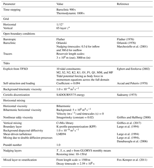
Flather (1976)Orlanski (1976)Marchesiello et al. (2001)Egbert and Erofeeva (2002)Accad and Pekeris (1978)Sadourny (1975)Griffies and Hallberg (2000)Griffies et al. (2017)Large et al. (1994)Large et al. (1994)Large et al. (1994)Danabasoglu et al. (2006)Fox-Kemper et al. (2011)

Table 1 Physical configuration, parameterization, and parameter choices for CARIB12.

CARIB12 uses a baroclinic time step of 900 s and a thermodynamic time step of 1800 s. The background kinematic viscosity of the interior is set to $\mathrm{1}\times {\mathrm{10}}^{-\mathrm{6}}$ m² s⁻¹. CARIB12 uses a Smagorinsky horizontal viscosity with a Smagorinsky constant of 0.02 and a bi-harmonic viscosity set to 5×10⁸ m⁴ s⁻¹. The configuration of the horizontal viscosity was determined after exploring different options and combinations within MOM6, including the use of a Laplacian viscosity and different values for the corresponding constants. The final configuration was largely determined by the mean flows into the CS across the multiple passages between the Caribbean islands, recognizing the importance of these flows in driving processes and variability within the CS. Vertical mixing is specified via the CvMix library (Griffies et al., 2017), with a background diapycnal diffusivity of $\mathrm{1}\times {\mathrm{10}}^{-\mathrm{6}}$ m² s⁻¹. CvMix utilizes the K-profile parameterization (KPP) of Large et al. (1994) for the boundary layer parameterization, with mixing due to double-diffusion and shear-driven turbulence. The parameterization of Fox-Kemper et al. (2011) is implemented for the re-stratification of the mixed layer by sub-mesoscale eddies with a front length scale of 1500 m. Additional details regarding the physical configuration and choice of parameterizations in CARIB12 are given in the following sub-sections and summarized in Table 1.

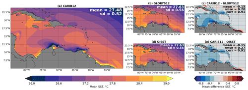
Figure 2 Time mean SST (°C) in the region of interest for this study (green box in Fig. 1) during 2000–2020. (a) CARIB12, (b) GLORYS12, (c) CARIB12 minus GLORYS12, (d) OISST, and (e) CARIB12 minus OISST. Mean and standard deviation are shown for each product (a, b, d). The mean bias, root mean squared error (RMSE), and spatial correlation (corr) are shown in each comparison panel (c, e).

The CARIB12 configuration has several key differences with other recent MOM6 configurations that cover a similar region, like the NWA12 configuration of Ross et al. (2023). For instance, the coupling infrastructure used in CESM–MOM6 is the Community Mediator for Earth Prediction Systems (CMEPS), whereas NWA12 uses the Flexible Modeling System (FMS) coupler. In terms of the physical configuration, a few distinctions are worth highlighting. The vertical mixing parameterizations are entirely different. As CARIB12 is a CESM–MOM6 configuration, we use KPP for the boundary layer mixing parameterization, which is the same scheme used in CESM (Large et al., 1994; Danabasoglu et al., 2020). On the other hand, NWA12 uses the energetics-based planetary boundary layer (ePBL) scheme of Reichl and Hallberg (2018). Vertical mixing in CARIB12 is specified via the CvMix library, which parameterizes vertical mixing in the interior using schemes that are different to those in NWA12 (Griffies et al., 2017). For example, shear-driven mixing in CARIB12 is handled by the parameterization of Large et al. (1994), whereas NWA12 applies the Jackson et al. (2008) scheme.

2.1.1 Initial and open-boundary conditions

Initial conditions are prescribed from the GLORYS12V1 reanalysis (GLORYS12; Jean-Michel et al., 2021). The GLORYS12 data are on a $\mathrm{1}/\mathrm{12}\mathit{°}$ resolution grid with 50 vertical levels. The model grid has two open boundaries, with one to the east and one to the north (Fig. 1a). The open-boundary conditions are specified daily using temperature, salinity, sea surface height (SSH), and meridional (v) and zonal (u) velocity components from GLORYS12. In total, 10 tidal constituents are specified at the boundaries, with tidal potential forcing included as a body force in the momentum equations. The tidal amplitudes and phases were obtained from the TPXO Global Tidal model 9v5a (Egbert and Erofeeva, 2002). Effects of self-attraction and loading are accounted for using the scalar approximation of Accad and Pekeris (1978) with a coefficient of 0.094. The barotropic flow at the boundaries is treated with a Flather boundary condition (Flather, 1976). The baroclinic component is specified using the Orlanski (1976) boundary condition. The boundary flows are nudged to exterior velocities at timescales of 0.3 d for inflow and 360 d for the outflow. Nudging layers for temperature, salinity, and velocities are applied to minimize noise at the boundaries that may contaminate the interior. The layers are based on mean monthly fields from GLORYS12. Damping in the nudging layers decays across 15 grid points away from the boundaries (dashed white lines in Fig. 1a) with maximum damping applied at the boundary grid cells. Damping at each point i is given by damping${}_i=\frac{\mathrm{1}}{\mathrm{dmin}+\mathrm{dr}*i}$, where $\mathrm{d}r=(\mathrm{dmax}-\mathrm{dmin})/(\mathrm{npts}+\mathrm{1})$, dmax=20 d, dmin=2 d, and npts=15 (corresponding to the number of points across which damping decays). The resulting equivalent restoring time from the applied nudging is of the order of 10 d (at the boundaries) and 150 d (at the farthest specified point from the boundary). The parameters for the applied damping were determined as a balance between reducing noise at the open boundaries and not influencing the solution towards the center of the domain. In general, low-resolution climate simulations, like those that will be downscaled using CARIB12, do not have high-frequency mesoscale variability that would be drastically attenuated by the applied nudging. Furthermore, the nudging will help prevent the formation of artificial currents and temperature/salinity signals along the boundaries. Nevertheless, as with any model, the nudging layers and other parameters might need to be revisited, depending on the climate simulation being downscaled.

2.1.2 Additional forcings

The atmospheric forcing is prescribed from the Japanese 55-year reanalysis (JRA55-do; Tsujino et al., 2018) and is specified every 3 h. Surface air temperature, downwelling shortwave radiation, downwelling longwave radiation, zonal and meridional wind, specific humidity, sea level pressure, and precipitation all referenced to 10 m above sea level in combination with sea surface temperature (SST), and surface velocities are used to compute surface fluxes of heat, water, and momentum using the Large and Pond (1981) bulk formula. The JRA55-do was developed following the Ocean Model Intercomparison Project protocol and is also used for many of the CESM simulations that will be downscaled with CARIB12. Freshwater runoff input is generated using the Global Flood Awareness System (GloFAS; Zsoter et al., 2021). The CESM climatological data river model was modified to use with the GloFAS data. The daily runoff is specified every 3 h with the atmospheric forcing and is spread horizontally across a maximum radius of 600 km. From the grid point, the runoff is prescribed with an e-fold scale of 200 km. The maximum radius for the spreading and the e-fold scale were determined through an ad hoc process by testing different combinations of these parameters. The combination specified here resulted in improved biases in salinity. A monthly climatology of surface chlorophyll a (chl a) is provided from the Sea viewing Wide Field-of-view Sensor (SeaWiFS) satellite mission (NASA Ocean Biology Processing Group, 2018) for the Manizza et al. (2005) opacity scheme.

2.2 Validation datasets

For the model validation, we use several datasets. These include the same GLORYS12 ocean reanalysis (Jean-Michel et al., 2021) used for the open boundaries and for the initial conditions. The reanalysis uses the CORAv4.1 database (Cabanes et al., 2013) to assimilate observations of sea level anomalies, sea surface temperatures (SSTs), and in situ profiles of temperature and salinity from Argo floats (Argo, 2000), shipboard eXpendable BathyThermograph (XBT), and conductivity–temperature–depth (CTD). Daily fields of temperature, salinity, mixed-layer depth (MLD), sea surface height (SSH), and velocities are used to validate CARIB12. Additionally, we validate the mixed-layer depth (calculated using the Δ0.03 kg m⁻³ density criterion) with the climatology of de Boyer Montégut et al. (2004). Altimetry-derived geostrophic currents with Ekman flow corrections from modeled fields from the GlobCurrent product (Rio et al., 2014) are used to validate the surface velocities and eddy kinetic energy field. The eddy kinetic energy was calculated as follows: $\mathrm{EKE}=\left(\frac{\mathrm{1}}{\mathrm{2}}\right)({u^{\prime }}^{\mathrm{2}}+{v^{\prime }}^{\mathrm{2}})$, where u^′ and v^′ are velocity anomalies resulting from decomposing the velocities into a mean velocity ($\stackrel{\mathrm{‾}}{u}$ and $\stackrel{\mathrm{‾}}{v}$) and the anomaly $u=\stackrel{\mathrm{‾}}{u}+u{}^{\prime }$.

Further validation is done for sea surface temperature (SST) fields against the Optimum Interpolation SST dataset (Huang et al., 2021) and, for sea surface salinity (SSS) fields, against the Multi Observation Global Ocean Sea Surface Salinity product (Droghei et al., 2016). The errors associated with the Multi Observation Global Ocean Sea Surface Salinity product used here are quite small (of the order of 10⁻³), even along the coastlines, which provides a good baseline for our validation. The SST, SSS, and MLD are also compared to the 1° resolution CESM–POP configuration used for the Ocean Model Intercomparison Project phase 2 (Tsujino et al., 2020).

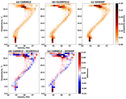
We have additionally validated water mass representation in the model against ship-based observations (CCHDO Hydrographic Data Office, 2023), using the Argovis application programming interface (Tucker et al., 2020), to identify World Ocean Circulation Experiment (WOCE) lines within the region of interest (i.e., WOCE lines A20 and A22; Fig. 1b) and for specific cruises within the time frame of the simulation (2000–2020). Profiles of temperature and salinity corresponding to the closest profile in time and space to each ship-based profile were extracted from the CARIB12 solution and the GLORYS12 reanalysis. The cruise profiles and CARIB12 and GLORYS12 profiles were binned in 0.2 PSU ×1 °C bins after being vertically interpolated onto a common grid to generate joint probability functions of temperature–salinity diagrams for each dataset. A total of 250 profiles from the following cruises are used in the analysis presented here: 43 profiles from 35A3200304, 43 profiles from 316N200309, 71 profiles from 316N200310, 43 profiles from 33AT20120324, and 50 profiles from 33AT20120419.

Jean-Michel et al. (2021)Huang et al. (2021)Droghei et al. (2016)Mercator Ocean (2021)Rio et al. (2014)de Boyer Montégut et al. (2004)Tsujino et al. (2020)

Table 2 Summary of datasets used in the validation of CARIB12 with their corresponding information.

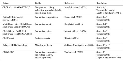
The dataset with an asterisk (^*) is also used for the model forcing.

When comparing our model to different data products, the dataset with a higher resolution was bi-linearly interpolated onto the horizontal grid of the product with lower resolution using the xESMF Python package (Zhuang et al., 2023). The CARIB12 solution was also saved at the runtime on the GLORYS12 vertical grid, and the ship-based profiles were re-gridded onto that same vertical grid. As this configuration has been developed for dynamical downscaling of climate simulations, validating seasonal to inter-annual variability is the target benchmark, and the overall validation focuses on these timescales. A summary of the validation datasets and relevant information is included in Table 2.

3 Results

3.1 Near-surface fields

In the following sub-sections, we examine temperature, salinity, sea level, and kinetic energy in the shallowest layer of the model (0–2.5 m) within the domain of interest (the region shown in Fig. 1b), as described in Sect. 2. Our focus is on time-averaged fields, with the average computed for the full time series or specific seasons.

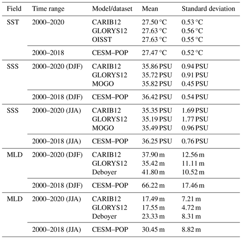
Table 3 Summary of mean and standard deviation of SST, SSS, and MLD for CARIB12 and GLORYS12 observational products and CESM–POP. Note that the CESM–POP simulation ends in 2018.

3.1.1 Temperature and salinity

Within the domain of interest (Fig. 1b), CARIB12 has a mean surface temperature of 27.5 °C, with a spatial standard deviation of 0.52 °C (Fig. 2a). The spatial patterns of temperature across the domain are well represented, and CARIB12 captures the upwelling system in the southern CS. The GLORYS12 reanalysis mean SST is 27.6 °C, with a standard deviation of 0.56 °C (Fig. 2b). These statistics indicate good agreement and similar distributions between CARIB12 and the GLORYS12 reanalysis, with a small and cold mean spatial bias of −0.15 °C (Fig. 2c). The optimum interpolation sea surface temperature (OISST) data have a mean SST of 27.6 °C and standard deviation of 0.55 °C (Fig. 2d). CARIB12 shows biases against OISST similar to those in the comparison to GLORYS12, with the mean bias of −0.15 °C being dominated by biases in shallow areas and within the CS (Fig. 2e). CARIB12 compares favorably against both datasets not only in terms of time mean but also for seasonal changes; a correlation very close to one is found between the CARIB12 12-month climatology and the 12-month climatology based on other products (Fig. A1). Also, differences between the CARIB12 standard deviation for the 12-month climatology and the standard deviation in other products are generally within ≈10 % of the values in the products used for validation (Fig. A2). The low-resolution CESM–POP simulation represents the broad patterns and mean SST within the region of interest (Table 3). However, it lacks proper representation of the extent and magnitude of features characteristic of the CS such as, for example, the magnitude of the upwelling system off the coast of South America (Fig. A3a).

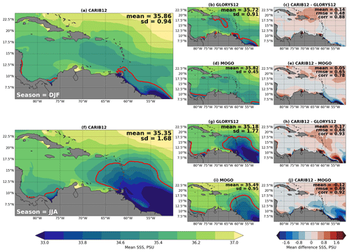
Figure 3 Time mean winter (a–e) and summer (f–j) SSS (PSU) in the region of interest for this study (green box in Fig. 1). (a, f) CARIB12, (b, g) GLORYS12, (c, h) CARIB12 minus GLORYS12, (d, i) MOGO, and (e, j) CARIB12 minus MOGO for winter and summer, respectively. The red line in panels (a), (b), (d), (f), (g), and (i) shows the 35 PSU isohaline as a proxy for the extent of the freshwater plumes from the Amazon and Orinoco rivers. Mean and standard deviation are shown for each product and seasonal mean. The mean bias, root mean squared error (RMSE), and spatial correlation (corr) are shown in each comparison panel.

The spatial patterns of SSS in different seasons are consistent between CARIB12 and both GLORYS12 and MOGO observational datasets (Fig. 3). Figure 3a–e show the mean winter (December–February, DJF) SSS for CARIB12 and the validation datasets; the spatial mean in CARIB12 is 35.86 PSU, with a mean bias of 0.14 PSU compared to GLORYS12 (Fig. 3a and c) and a bias of 0.05 PSU compared to the MOGO observational dataset (Fig. 3e). Notably, GLORYS12 appears to have a freshwater source in the region of the Dominican Republic and Puerto Rico, thus resulting in positive biases within the CS. This is highlighted by the red contour line corresponding to 35 PSU shown in Fig. 3b. During the summer (June–August, JJA), CARIB12 shows a mean bias of 0.17 PSU compared to GLORYS12 and one of −0.12 PSU compared to MOGO (Fig. 3j). The 35 PSU contour line (red line in Fig. 3) delineates the freshwater salinity front (based on the discussion in Seijo-Ellis et al., 2023) and shows that the spread and extent of the plume waters is similar between CARIB12 and GLORYS12 but is much smaller in the gridded observations (particularly during the winter; Fig. 3a–e).

The seasonal spread of the low-salinity plume from the Amazon and Orinoco rivers is well captured, with peak high salinity during the winter months within the CS and minimum salinity during the summer months (Fig. B2a). The largest biases in SSS are the areas of major riverine inputs, namely the Amazon and Orinoco rivers. These biases may arise from the specification of the river runoff to the ocean and how mixing of the freshwater input in the ocean is handled in CARIB12 (and, e.g., differences with the corresponding choices in GLORYS12). In CARIB12, runoff is not distributed vertically in the ocean but rather spread horizontally across a maximum radius of 600 km, with an e-fold decay scale of 200 km at the shallowest layer. Also, some of the large biases when comparing to observations may arise due to limited observations in the shallow-shelf regions and the interpolations done to grid the data. Nevertheless, the seasonal SSS is well represented in CARIB12, with good correlations between datasets and smaller biases within the Caribbean Sea away from riverine sources. Known pathways of Amazon River waters into the CS are well reproduced, as evidenced by a backtracking experiment (see Appendix B). The smallest SSS biases are generally found within the CS, which indicate that CARIB12 is performing well within the region of interest. Correlation close to one is found between the CARIB12 12-month climatology and the 12-month climatology, based on other products, in most of the domain (Fig. A4); also, within the CS, differences between the CARIB12 standard deviation for the 12-month climatology and the standard deviation in other products are generally within ≈25 % of the values in the products used for validation, except in the western part of the basin (Fig. A6).

In contrast to the well-simulated variability in SSS in CARIB12, the low-resolution CESM–POP simulation exhibits biases that hinder the model's performance to properly represent the SSS variability within the Caribbean Sea (Table 3 and Fig. A3b and c). There is an overall positive salinity bias irrespective of the season, and the extent and magnitude of the Amazon and Orinoco river plumes are not well represented. These biases may be a product of several factors: biases in the specification of the river runoff, inadequate representation of sub-grid-scale process and mesoscale eddies that play an important role in the spreading of the river runoff and salinity variability in the region, and/or biases inherent to the low resolution of the model.

3.1.2 Surface currents speed, eddy kinetic energy, and sea surface height

The mean winter and summer surface speed is shown in Fig. 4. The direction and spatial distribution of the near-surface flows is well represented in CARIB12 compared to GLORYS12 and the GlobCurrent product (arrows in Fig. 4). The mean winter speed in CARIB12 is 0.19 m s⁻¹, which corresponds to a mean bias of ≈0.02 m s⁻¹ below the mean speed in GLORYS12. Compared to the GlobCurrent product, biases are overall larger, with a mean negative bias of 0.07 m s⁻¹. The biases are within the same order of magnitude during the summer and show overall similar structures to the biases during the winter (Fig. 4).

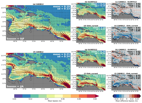
Figure 4 Time mean winter (a–e) and summer (f–j) surface speed (m s⁻¹) in the region of interest for this study (green box in Fig. 1). (a, f) CARIB12, (b, g) GLORYS12, (c, h) CARIB12 minus GLORYS12, (d, i) GlobCurrent, and (e, j) CARIB12 minus GlobCurrent for winter and summer, respectively. Black arrows show the direction of the surface flow, with the size of the arrows scaled by the magnitude of the speed. Mean and standard deviation are shown for each product and seasonal mean. The mean bias, root mean squared error (RMSE), and spatial correlation (corr) are shown in each comparison panel.

The largest biases during both seasons when compared to GLORYS12 occur along the region southwest of Hispaniola where two jets converge, namely the main Caribbean Current and the jet around 18° N (Chérubin and Richardson, 2007). The biases in this area are of the order of up to ≈0.12 m s⁻¹. This region is one of increased shear with rapidly varying bottom topography. Thus, the difference in the topography between the models and the specification of the horizontal viscosity may be driving these biases. The speed compares well elsewhere in the region of interest, including the narrow passages in the eastern CS. This indicates that CARIB12 represents the surface inflow to the CS and the flows associated with the advection of the freshwater plumes from the Amazon and Orinoco rivers well. The biases are larger when comparing CARIB12 to the altimetry- and model-based GlobCurrent (Fig. 4e and j), but it is worth noting the difference in spatial resolutions and that the correction for Ekman flows is model-based, which may have its own biases for a small and under-sampled region like the CS. This is a worthy distinction because surface Ekman currents can reach 0.5 m s⁻¹ in parts of the Caribbean Basin (Andrade-Amaya, 2000). The seasonal variability in the flow speed is well represented in CARIB12, with higher mean speeds in the summer and the lowest mean speeds during the winter, and this is evidenced by the eddy kinetic energy fields (Fig. 5). In particular, CARIB12 captures the strengthening of the Caribbean Current during the boreal summer months (JJA), as well as the re-circulation that occurs within the Colombian basin.

The seasonal eddy kinetic energy (EKE) for CARIB12, GLORYS12, and from the GlobCurrent product is shown in Fig. 5; an overall mean negative bias is observed irrespective of the season and is most notable in the summer, when EKE is larger (Jouanno et al., 2012). These biases are particularly noticeable south of Hispaniola and in the southwest corner of the CS, where a re-circulation of the surface flow occurs. Despite the lower EKE, seasonal variability is well represented in CARIB12, and the spatial variability compares well with GLORYS12 and the altimetry-derived product (Fig. 5c–e). The seasonal increase in EKE during the summer months is captured, although mesoscale patterns are not well represented. In particular, the increase in EKE extending westward across the Caribbean Sea (65 to 80° W) is not as strong in CARIB12 as GLORYS12 and the GlobCurrent product suggests. The 20-year time mean EKE biases (not shown) are of the same order of magnitude as the seasonal EKE biases, indicating that the seasonal biases are dominated by biases in the long-term mean. Further improvements in parameter choices may help reduce some of these biases and improve the representation of mesoscale variability.

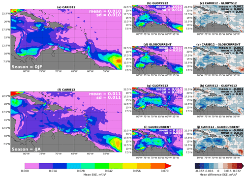
Figure 5 Time mean winter (a–e) and summer (f–j) EKE (m² s⁻²) in the region of interest for this study (green box in Fig. 1). (a, f) CARIB12, (b, g) GLORYS12, (c, h) CARIB12 minus GLORYS12, (d, i) MOGO, and (e, j) CARIB12 minus MOGO for winter and summer, respectively. The red line in panels (a), (b), (d), (f), (g), and (i) shows the 35 PSU isohaline as a proxy for the extent of the freshwater plumes from the Amazon and Orinoco rivers. Mean and standard deviation are shown for each product and seasonal mean. The mean bias, root mean squared error (RMSE), and spatial correlation (corr) are shown in each comparison panel.

Figure 6 shows the winter and summer mean SSH anomalies (SSHa; spatial mean removed) for CARIB12 and GLORYS12. The winter mean SSHa in CARIB12 is −0.002 m and compares well with the mean in GLORYS12 (Fig. 6a–c); similarly, a good comparison is seen for the summer (Fig. 6d–f). The difference in both seasons indicates an overall more positive SSHa in CARIB12. The regions of positive biases in surface speeds (Fig. 4) correspond to regions where the horizontal SSHa gradient is stronger in CARIB12, and vice versa, where the biases in speed are negative (for example, southeast of Hispaniola around 16° N and 75° W). The SSHa within the region of interest is characterized by a negative SSHa structure along the shelf waters of South America, whose meridional gradient delineates the location of the Caribbean Current. The meridional extent of this feature extends further offshore in CARIB12, indicating a wider Caribbean Current in CARIB12 compared to GLORYS12. The standard deviations and correlations (Fig. 6) show reasonable consistency between the solutions CARIB12 and GLORYS12. CARIB12 also reproduces the seasonality of SSHa well, with stronger meridional gradients and variability during the boreal summer compared to winter driving the intensification of the surface flows as described before. This seasonal cycle is also intrinsically connected to the seasonal variability in SSS (driven by the freshwater plumes of the Amazon and Orinoco rivers). While not shown, a simple comparison of the SSHa time series with tidal gauges was completed and shows general good agreement with stations across the Caribbean Sea and Gulf of Mexico.

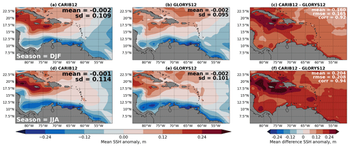
Figure 6 Time mean winter (a–c) and summer (d–f) SSH anomaly (SSHa, m) in the region of interest for this study (green box in Fig. 1). (a, d) CARIB12, (b, e) GLORYS12, and (c, f) CARIB12 minus GLORYS12 for winter and summer, respectively. The SSHa is the time mean SSH minus the spatial mean. Mean and standard deviation are shown for each product and seasonal mean. The mean bias, root mean squared error (RMSE), and spatial correlation (corr) are shown in each comparison panel.

3.2 Mixed-layer depth

We compare the winter and summer mixed-layer depth (MLD) against the GLORYS12 reanalysis and the climatology by de Boyer Montégut et al. (2004). As detailed in Sect. 2, the calculation is done using the Δ0.03 kg m⁻³ density criterion with respect to surface values. CARIB12 compares favorably against GLORYS12 (Fig. 7). The mean bias in the winter is 2.5 m, indicating an overall deeper MLD in CARIB12, with a RMSE of 6.31 and correlation of 0.89. In the summer, CARIB12 has a slightly shallower MLD than GLORYS12, with a mean bias of −0.13 m, RMSE of 3.71, and correlation of 0.89. The biases within the Caribbean Sea and away from the vicinity of the Amazon and Orinoco rivers are attributable to the small biases described for salinity; an overall positive salinity bias (Fig. 3) corresponds to saltier waters in the near-surface, which leads to weaker vertical stratification (Fig. 9) in the upper 0–100 m and results in a deeper mixed layer, particularly during the winter. In both seasons, the mean MLD from CARIB12 is closer to the mean of the de Boyer Montégut et al. (2004) climatology than GLORYS12. A likely contributor to this improvement could be the added effect of tides in CARIB12 driving vertical mixing, a process that is not included in GLORYS12.

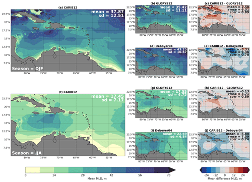
Figure 7 Time mean winter (a–e) and summer (f–j) MLD (m) in the region of interest for this study (green box in Fig. 1). (a, f) CARIB12, (b, g) GLORYS12, (c, h) CARIB12 minus GLORYS12, (d, i) Deboyer, and (e, j) CARIB12 minus Deboyer for winter and summer, respectively. Mean and standard deviation are shown for each product and seasonal mean. The mean bias, root mean squared error (RMSE), and spatial correlation (corr) are shown in each comparison panel.

When comparing the MLD against the de Boyer Montégut et al. (2004) climatology, CARIB12 has an overall shallower MLD across seasons. During the winter, the mean MLD bias is −5.24 m, with a RMSE of 9.53 and correlation of 0.78. During summer, the bias is −6.58 m, with a RMSE of 8.03 and correlation of 0.83. CARIB12 represents the MLD seasonality across the domain well; the mixed layer is deepest in winter and becomes shallower during the spring as temperatures rise and the Amazon and Orinoco river plumes influence the Caribbean region. The mixed layer is overall shallowest during the summer months before deepening again in the fall as near-surface temperatures decrease and salinity increases in the absence of the Amazon and Orinoco river plumes. Overall, CARIB12 captures both the seasonal variability and spatial patterns of the MLD and compares well to GLORYS12.

The CESM–POP-simulated MLD shows biases of the order of 13 m during the summer and 30 m during the winter for the mean MLD (Table 3 and Fig. A3d–e). These biases in CESM–POP could be in part attributed to unresolved processes and the biases in salinity (Sect. 3.1.1); a positive salinity bias leads to weaker vertical stratification and thus an overall deeper mixed layer (Fig. A3). While the broad spatial patterns of MLD during the summer agree with those in CARIB12 and other datasets, the patterns during the winter do not appear to be as well represented in the CESM–POP simulations and further highlight the important role of Amazon River runoff and salinity in the Caribbean Sea (Fig. A3d and e). The biases in the CESM–POP-simulated MLD are larger than those compared to CARIB12 and GLORYS12, highlighting the importance of processes across scales to properly resolve regional mixed-layer depths but also the sensitivity of the definition of MLD and vertical grids in the models (Treguier et al., 2023).

Figure 8 Temperature–salinity joint probability density function for (a) CARIB12, (b) GLORYS12, and (c) GO-SHIP. Panel (d) shows the difference between panels (a) and (b). Panel (e) shows the difference between panels (a) and (c).

3.3 Vertical structure and water mass properties

We compare the vertical structure of the water column in CARIB12 with GLORYS12 and with available observations along WOCE lines A20 and A22 within the region of interest (Fig. 1b). Figure 8 shows joint probability functions of temperature–salinity for CARIB12, GLORYS12, and GO-SHIP CTD data (Fig. 8a–c, respectively; CARIB12 and GLORYS12 data are co-located in space and time with profiles along the WOCE lines); the overall vertical structure and water mass characteristics is well represented in CARIB12, with some of the largest differences occurring in the Caribbean surface waters (Fig. 8d–e). These differences are not surprising; surface waters exhibit higher variability as they are exposed to a number of large-scale circulation and forcing mechanisms, e.g., the influence of river runoff at sub-seasonal to seasonal scales, wind-driven circulation, eddies, and the Caribbean Current (Corredor and Morell, 2001; Jouanno et al., 2012; Digna et al., 2018; Seijo-Ellis et al., 2023). Additional biases are noted around the salinity maximum (sub-tropical underwater (SUW), as described in, e.g., Seijo-Ellis et al., 2019; Torres et al., 2023), where there is a wider spread in values in CARIB12 compared to GLORYS12 and GO-SHIP. Nevertheless, the biases in the sub-surface salinity maximum are small, and the model shows good agreement with GLORYS12 and observations. These differences may reflect larger variability in the sub-surface inflow associated with the North Atlantic Gyre and/or the formation of the SUW mass in the North Atlantic.

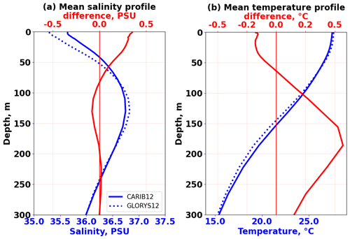
Figure 9 Time mean salinity (a) and temperature (b) profiles for the area average within the region of interest for this study (green box in Fig. 1). CARIB12 (solid blue line) and GLORYS12 (dotted blue line) are shown. The difference between the two products is shown in red.

A comparison between CARIB12 and GLORYS12 for the area-weighted time mean profile of salinity and temperature in the region of interest (Fig. 9) shows a salty and slight cold bias near the surface (consistent with the discussion in Sect. 3.1). At depth, the biases are reversed with a fresh bias in the 100–150 m depth range, which corresponds to the sub-surface salinity maximum associated with sub-tropical underwater, and a warm bias of up to 0.5 °C. Biases in the mean profiles of temperature and salinity get smaller with depth (Fig. 9). Biases seen in Fig. 9 are representative of the biases in Figs. 10 and 11, which show that CARIB12 reproduces the large-scale signals in both temperature and salinity well across the length of the simulation.

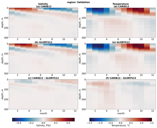
Figure 10 Area-weighted mean seasonal salinity anomalies within the validation region (green box in Fig. 1). (a) CARIB12, (b) GLORYS12, and (c) the difference between the products. Area-weighted mean seasonal temperature anomaly within the validation region, with (d) CARIB12, (e) GLORYS12, and (f) the difference between the products.

The area-weighted seasonal cycle of salinity and temperature in CARIB12 is in good agreement with GLORYS12 (Fig. 10). Model biases indicate that the amplitude of the seasonal cycle in CARIB12 is well represented compared to GLORYS12. The near-surface biases in the seasonal cycle of temperature and salinity are of the same order as those shown in Sect. 3.1. Figure 10a–c show the strong seasonal cycle in salinity for the region that is largely driven by the runoff from the Amazon and Orinoco rivers during late boreal spring through early fall and the higher salinity during late fall through winter into early spring driven by the lower riverine input to the ocean and the inflow of saltier Atlantic waters. These results highlight CARIB12's ability to correctly represent temperature and salinity variability in the CS and surrounding regions at seasonal scales.

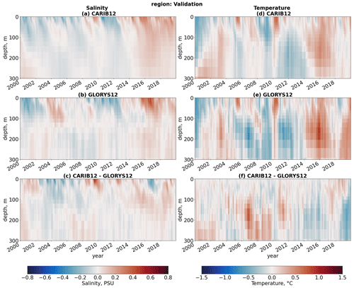
Figure 11 Area-weighted mean monthly salinity anomaly within the validation region (green box in Fig. 1), with (a) CARIB12, (b) GLORYS12, and (c) the difference between the products. Area-weighted mean seasonal temperature anomaly within the validation region, with (d) CARIB12, (e) GLORYS12, and (f) the difference between the products.

Figure A7 shows the seasonal anomalies in salinity (Fig. A7a–c) and temperature (Fig. A7d–f) for the sub-region east of the Lesser Antilles (see sub-regions in Fig. A5). CARIB12 reproduces the signals of temperature and salinity of the waters well outside the eastern CS. The largest salinity biases (≈25 %) occur near the surface during the summer months, which agree well with the biases shown in Fig. 3. These biases are reduced at depth. The temperature biases in this sub-region remain below (≈10 %). Within the eastern Caribbean Sea (region CS.E in Fig. A5), the salinity biases are reduced below ≈25 %, and the temperature biases remain below ≈10 %. This indicates that salinity biases resulting from the limitations in the specification of the freshwater runoff are drastically reduced as the waters enter the CS, which is the main region of interest in the development of CARIB12.

At inter-annual timescales, CARIB12 salinity and temperature anomalies in the upper 300 m are overall consistent with GLORYS12 (Fig. 11). The largest anomalies in GLORYS12 are also present in CARIB12, including signals likely associated with the 2015/2016 La Niña (salty and warm anomalies from 2015 onwards; Jiménez-Muñoz et al., 2016), and the biases associated with those signals are generally below ≈20 %. It is worth noting that the signals associated with these anomalies are not only captured in the horizontal mean of temperature and salinity; their vertical signature is also well represented in CARIB12. Within the CS (Fig. 12), inter-annual anomalies are also well captured in CARIB12, although differences in the magnitude and amplitude of some of the signals lead to larger biases when compared to the full validation region shown in Fig. 11. For example, the salty and warm signal between 2016 and 2020 has a longer duration in CARIB12, but the magnitude of the anomalies is not as large as in GLORYS12. The attenuation of these inter-annual anomalies may also be related to the specification of the horizontal viscosity parameters in the model and the added effect of tides in CARIB12 driving enhanced vertical mixing not represented in GLORYS12. Further evaluation of these effects is worth an additional examination but remains beyond the scope of this work.

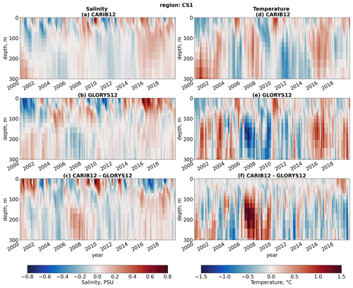
Figure 12 Area-weighted mean monthly salinity anomaly within the CS (CS1 in Fig. A5). (a) CARIB12, (b) GLORYS12, and (c) the difference between the products. Area-weighted mean seasonal temperature anomaly within the validation region. (d) CARIB12, (e) GLORYS12, and (f) the difference between the products.

Smith et al. (2007)Johns et al. (2002)Johns et al. (2002)Gradone et al. (2023)Johns et al. (2002)Johns et al. (2002)Johns et al. (2002)Johns et al. (2002)Johns et al. (2002)Sheinbaum et al. (2002)Candela et al. (2003)Candela et al. (2019)

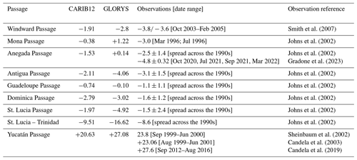
Table 4 Mean ocean transports (Sv) across passages in the Caribbean Sea. Estimates from CARIB12 and the GLORYS12 reanalysis are for the period 2000–2020. Estimates from observations are for the date ranges indicated in the table and are included together with relevant references. The location of each passage is shown in Fig. 1. Negative transports correspond to a westward or southward flow and positive transports to eastward or northward flows.

3.4 Transports

Proper representation of ocean mass transports into the CS is important to ensure the processes and properties within it are also well represented. Ocean mass transports were calculated for passages in the eastern and northern Caribbean Sea. The passages are shown in Fig. 1b, and a summary of the mean transports in CARIB12, GLORYS12, and observational estimates can be found in Table 4 (for each of the passages of interest). We note that while transports based on CARIB12 and GLORYS12 are a time mean during 2000–2020, observational estimates are available only for shorter periods of time (often outside the 2000–2020 period of the simulation).

The mean transport across the Windward Passage between Cuba and Hispaniola is 1.91 Sv into the Caribbean Sea, which is lower than that in GLORYS12 (2.8 Sv) and in observation-based estimates ($\mathrm{3.8}/\mathrm{3.6}$ Sv) by Smith et al. (2007). Nevertheless, Johns et al. (2002) and Smith et al. (2007) indicate that there are still uncertainties in the transport through this passage.

The inflow across the Mona Passage (0.38 Sv) is also underestimated in CARIB12 compared to observations (3.0 Sv); here, GLORYS12 has a net outflow of 1.22 Sv, which, along with the freshwater shown for GLORYS in Fig. 3b (red contour in the region of the Dominican Republic and Puerto Rico), may be a significant contributor to the biases seen in the region when comparing CARIB12 to GLORYS12 (e.g., Fig. 3c).

Flow through the Anegada Passage is an important contributor to the circulation between the Atlantic and the Caribbean Sea; CARIB12 shows good agreement with observations by Johns et al. (2002), with a 1.53 Sv inflow compared to 2.5 Sv. However, recent studies suggest that the inflow through the Anegada Passage may be larger than previously thought (e.g., Gradone et al., 2023). CARIB12 captures the mean transport through the Anegada Passage better than GLORYS12, which has a mean outflow of 0.14 Sv.

The Antigua Passage mean inflow is 2.11 Sv in CARIB12, which compares favorably against 3.1 Sv estimated by Johns et al. (2002) and is about half the transport in GLORYS12 (−4.06 Sv). Across the Guadeloupe Passage, the inflow in CARIB12 (0.74 Sv) agrees better with observations (1.1 Sv) than GLORYS12 (0.10 Sv). This is similar for the Dominica Passage, although CARIB12 (2.79 Sv) and GLORYS12 (3.02 Sv) overestimate the inflow here compared to 1.6 Sv inflow estimated by Johns et al. (2002). The St. Lucia Passage mean inflow in CARIB12 agrees well with observations (1.97 Sv in CARIB12 and 1.5 Sv from observations), while GLORYS12 overestimates the inflow by 3.4 Sv.

The St. Lucia – Trinidad section (Fig. 1b) is a combination of the St. Vincent and Grenada passages in Johns et al. (2002). CARIB12 has a mean inflow of 9.51 Sv, which agrees well with the 8.6 Sv estimate by Johns et al. (2002). Along this section, GLORYS12 has a mean inflow that is almost twice as large (16.62 Sv) as that suggested by observations, which may also contribute to near-surface biases in the CS (particularly the southern part) discussed in Sect. 3.1 and 3.1.2.

The net mean inflow to the Caribbean Sea is 20.94 Sv, which is 0.31 Sv more than the mean flow out of the Caribbean Sea via the Yucatán Channel (20.63 Sv) (Fig. 1). The mean flow through the Yucatán Channel in CARIB12 is ≈3 Sv less than that estimated from observations by Sheinbaum et al. (2002) and Candela et al. (2003) (23.8 and 23.06 Sv, respectively); it is also ≈7 Sv below GLORYS12 and the most recent estimate of 27.6 Sv by Candela et al. (2019). The difference in mean transport across observational estimates collected in different years may indicate a low-frequency variability that is not well-captured in CARIB12 and is partially captured in GLORYS12. Also, the estimates by Sheinbaum et al. (2002) and Candela et al. (2019) are based on observations between September 1999 and June 2001, whereas the estimate in Candela et al. (2019) is based on observations between September 2012 and August 2016. We also note that the section defining the Yucatán Channel in CARIB12 is not completely bounded by land, which may result in a lower mean outflow there.

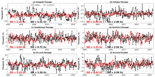
Figure 13 Transport through passages in the eastern Caribbean Sea. Monthly anomalies from CARIB12 (red) and GLORYS12 (black) for the (a) Anegada Passage, (b) Antigua Passage, (c) Guadeloupe Passage, (d) Dominica Passage, (e) St. Lucia Passage, and (f) the St. Lucia – Trinidad transect. The standard deviation of the time series is indicated at the bottom of each panel and color coded by product. Time mean transports for each passage can be found in Table 4 for both CARIB12 and GLORYS12, as well as available observations.

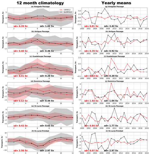
Figure 14 Transport through passages in the eastern Caribbean Sea from CARIB12 (red) and GLORYS12 (black). (a–f) Seasonal anomalies. (g–l) Yearly anomalies. In panels (a)–(f), the shading shows the standard deviation for each month (i.e., standard deviation of all January means and so on).

At sub-seasonal timescales, CARIB12 shows less variability compared to GLORYS12 (Fig. 13), which is reminiscent of the negative biases in the surface speed and EKE described in Sect. 3.1.2. At seasonal timescales, there is an overall agreement between CARIB12 and GLORYS12 (Fig. 14a–f). With the exception of the Guadeloupe and Dominica passages (Fig. 14c and d), GLORYS12 shows stronger seasonal variability than CARIB12. We note that, as the seasonal cycle is regulated by the seasonal freshwater runoff from the Amazon and Orinoco river plumes (Wilson and Johns, 1997; Corredor and Morell, 2001; Johns et al., 2002; Chérubin and Richardson, 2007; Jouanno et al., 2012; Seijo-Ellis et al., 2023), differences in how the runoff is represented in the two models (runoff is applied in the sub-surface in GLORYS12 vs. at the surface in CARIB12) may have implications for the across-passage transports and thus result in differences between CARIB12 and GLORYS12. Finally, GLORYS12 shows stronger inter-annual variability than CARIB12 (Fig. 14g–l). While the time mean flows are well represented in CARIB12 compared to observations, the model does not capture the same amplitude and frequency in flow variability that GLORYS12 suggests exists in some of the passages at sub-seasonal and inter-annual timescales (Figs. 13 and 14g–l). These differences may be further indicators of the differences between the models, namely runoff specification, horizontal viscosity configuration, and the overall differences in model forcing (i.e., GloFAS runoff in CARIB12 versus runoff climatology in GLORYS12). Continuous observations would be needed to better assess how CARIB12 and GLORYS12 represent variability across timescales in the transports across the numerous passages. Nevertheless, CARIB12 and GLORYS12 indicate that the flow across these passages is complex and highly variable, which has been highlighted by previous studies and remains an active area of research (Wilson and Johns, 1997; Johns et al., 1999; Centurioni and Niiler, 2003; Johns et al., 2002; Gradone et al., 2023).

4 Conclusions

A new regional ocean-only CESM–MOM6 configuration of the Caribbean Sea is validated for the present day (2000–2020) against the GLORYS12 reanalysis and a suite of observation-based datasets. Near-surface fields of temperature, salinity, and SSH are well represented, with small mean biases, comparable standard deviations, and high correlations between CARIB12, GLORYS12, and the respective observation-based datasets for each field. In particular, the seasonal cycle of SSS and the spatial pattern of the low salinity associated with the Amazon River plume is well captured. Eddy kinetic energy shows some negative biases within the Caribbean Sea, yet the seasonal variability is captured. The MLD is also well represented, with a deep-winter mixed layer and a shallow-summer MLD and biases against the GLORYS12 reanalysis generally <3 m. The mean flows are also well represented compared to observations, but CARIB12 shows lesser variability when compared to GLORYS12 flows and underestimates the mean Yucatán Channel transport. Further tuning of the horizontal viscosity and choice of parameters may be needed to improve the biases in near-surface fields, particularly regarding mesoscale variability across the Caribbean Sea.

The vertical structure of the water column is well captured in CARIB12 compared to GLORYS12 and GO-SHIP data. The largest differences are observed in the near-surface water mass and in the layer of the sub-surface salinity maximum, which, in CARIB12, is broader and not as pronounced as in the GLORYS12 reanalysis and GO-SHIP data. Nevertheless, the overall vertical structure is reproduced accurately in CARIB12. Vertical temperature and salinity variability is also overall well represented across timescales. While some differences exist at sub-seasonal timescales, the seasonal cycle is represented well. Across the full simulation, anomalies in temperature and salinity across the water column are comparable to those in the reanalysis.

Ocean mass transports across a number of passages in the northern and eastern Caribbean sea are computed and compared against GLORYS12 and observations. The mean flows in CARIB12 compare favorably against observations, while GLORYS12 exhibits some biases, particularly along the Mona Passage, Anegada Passage, and the St. Lucia – Trinidad section. The seasonal transports in CARIB12 compare overall well with the GLORYS12 reanalysis, yet GLORYS12 exhibits larger variability at sub-seasonal and inter-annual timescales. Nevertheless, there are no observations available that are long enough to assess the variability in the flows along the passages across different timescales.

We compared mean fields for SST, SSS, and MLD of CARIB12 against a 1° resolution CESM–POP configuration. While the CESM–POP captures the mean state and broad patterns of SST in the CS, it does not represent well the significant dynamical features that drive variability in the region. For example, the location, spatial extent, and magnitude of the Caribbean Current and the upwelling system in South America are not well represented. In addition, there are biases in SSS and the representation of the Amazon and Orinoco river plumes. The extent and seasonal amplitude of the SSS cycle is not well captured, including unresolved mesoscale and sub-mesoscale instabilities that drive much of the variability within the CS. These salinity biases may also be responsible for large biases seen in the mixed-layer depth, suggesting that the low resolution does not represent the regional vertical stratification and variability to a good degree. CARIB12 improves these biases significantly, highlighting the need for high-resolution regional models in order to properly address climate impacts at these scales and support decision-making.

The main biases in CARIB12 may be attributed to two sources. The first is the limitations in the specification of the freshwater runoff. The second is the need for further fine-tuning of the horizontal viscosity configuration and the need for higher-order parameterizations for high-resolution configurations like this one. CARIB12 is a test bed for the development of new schemes and parameterizations that can address these sources of biases and enhance the regional capabilities of CESM–MOM6.

With this thorough validation, we showcase the new capabilities within CESM to perform high-resolution regional ocean modeling. CARIB12 and the new regional ocean capabilities of CESM are invaluable tools for regional climate impact studies. As a community model configuration available to the wider scientific community, CARIB12 is a valuable tool for actionable science at regional scales and provides the foundation for the further development of regional ocean climate modeling and downscaling within CESM. For example, as part of a separate project, the CARIB12 configuration will be used for the dynamical downscaling of CESM climate projections to examine changes in the heat and salinity budgets of the Caribbean Sea under future climates.

Appendix A: Additional figures

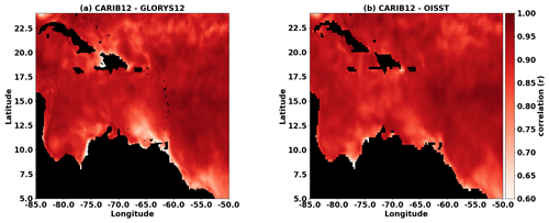
Figure A1 Correlation of the 12-month SST climatology between (a) CARIB12 and GLORYS12 and (b) CARIB12 and OISST.

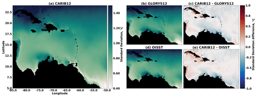
Figure A2 Standard deviation of the 12-month SST climatology from (a) CARIB12, (b) GLORYS12, and (d) OISST. (c) Difference between the standard deviations of CARIB12 and GLORYS. (d) Difference between the standard deviations of CARIB12 and OISST.

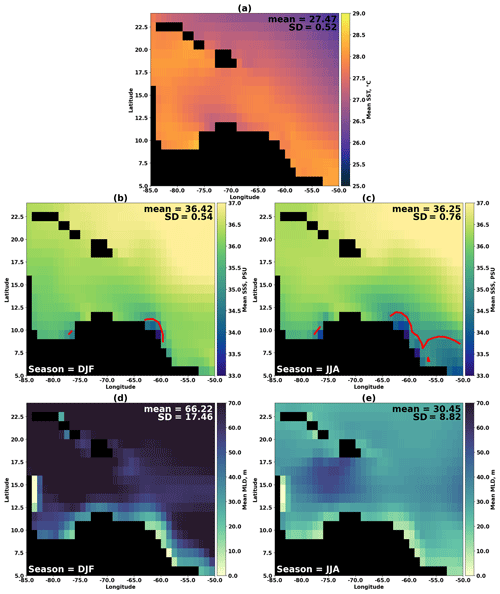
Figure A3 Mean fields and metrics for the 1° CESM–POP simulation within region of interest. (a) Time mean SST (2000–2018), (b) winter time mean SSS (2000–2018), (c) summer time mean SSS (2000–2018), (d) winter time mean MLD (2000–2018), and (e) summer time mean MLD (2000–2018). The red line in panels (b) and (c) corresponds to the 35 PSU contour line. Spatial means and standard deviations are specified in the inset text for each panel.

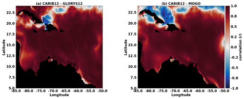
Figure A4 Correlation of the 12-month SSS climatology between (a) CARIB12 and GLORYS12 and (b) CARIB12 and MOGO.

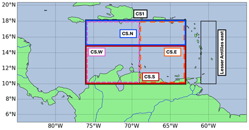
Figure A5 Sub-regions used for the additional validation of CARIB12. Region CS1 encompasses all four sub-regions (CS.N, CS.S, CS.E, and CS.W). Only validations for CS1, CS.E, and Lesser Antilles east are shown in addition to the full validation region shown in Fig. 1.

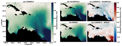
Figure A6 Standard deviation of the 12-month SSS climatology from (a) CARIB12, (b) GLORYS12, and (d) MOGO. (c) Difference between the standard deviations of CARIB12 and GLORYS. (d) Difference between the standard deviations of CARIB12 and MOGO.

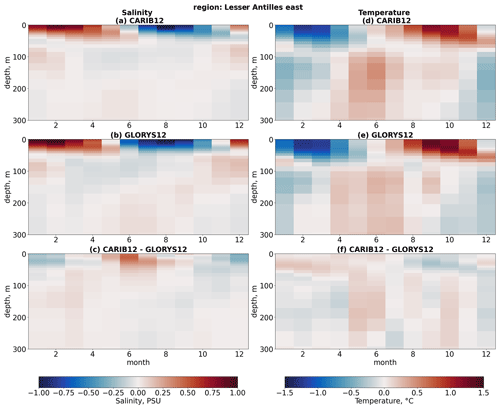
Figure A7 Area-weighted mean seasonal salinity anomalies within the Lesser Antilles east sub-region shown in Fig. A5. (a) CARIB12, (b) GLORYS12, and (c) the difference between the products. Area-weighted mean seasonal temperature anomaly within the validation region. (d) CARIB12, (e) GLORYS12, and (f) the difference between the products.

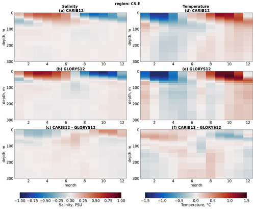
Figure A8 Area-weighted mean seasonal salinity anomalies within the eastern CS region (CS.E) in Fig. A5. (a) CARIB12, (b) GLORYS12, and (c) the difference between the products. Area-weighted mean seasonal temperature anomaly within the validation region. (d) CARIB12, (e) GLORYS12, and (f) the difference between the products.

Appendix B: Representation of known Amazon River pathways into the Caribbean Sea in CARIB12

As described in Sect. 1, variability within the Caribbean Sea (CS) is closely linked to the influence of the Amazon and Orinoco river plumes. This includes control over near-surface salinity, stability of the Caribbean Current, the generation of mesoscale eddies, and the modulation of the seasonal eddy kinetic energy across the CS (Chérubin and Richardson, 2007; Jouanno et al., 2012; Grodsky et al., 2015; Seijo-Ellis et al., 2023). A regional configuration of the CS, such as CARIB12, must properly capture the pathways and timing of plume waters entering the CS. We perform a case study validation of CARIB12 using the Lagrangian particle-tracking model OceanParcels (Lange and Sebille, 2017; Delandmeter and Sebille, 2019). We replicate the methodology and experiment performed by Seijo-Ellis et al. (2023) to examine the origin and pathways of waters arriving to the Virgin Islands basin (VIB). In total, 100 passive particles were released daily at the grid point closest to 18° N, 64.8° W; i.e., the closest point to site Bi14 in Seijo-Ellis et al. (2023) and backtracked for 100 d. Backtracking is done via a fourth-order Runge–Kutta interpolation scheme using the CARIB12 daily surface velocity fields. This approach allows us to trace the trajectories of the particles 100 d before their arrival to the release site. While we only show the year 2010 as an example (which also allows a comparison to the results shown in Figs. 5 and 6 of Seijo-Ellis et al., 2023), the backtracking was completed for the length of the simulation for the years 2000–2020.

The analysis of the trajectories follows the same method described in Seijo-Ellis et al. (2023) and is summarized in Fig. B1. For each arrival date (same as release date when backtracking), we count the number of trajectories within 0.2°×0.2° bins (Fig. B1a). Two main constraints are enforced, where particles with more than one position recorded in the same bin are only counted once if a particle passes through but has no recorded position in a particular bin it is not counted. A probability density map of the trajectories of the particles 100 d prior to their release is then generated for each release date (Fig. B1a and b). In order to summarize the temporal evolution of these binned trajectory maps, we generate a time series of the cumulative number of trajectories per bin color-coded by each bin's location (Fig. B1c–e). The first step is to color code the bins by their location, such that a change in color represents a meridional change in position and a change in color shading represents a latitudinal change in position (Fig. B1c). For each release date, color-coded bins are stacked on top of each other according to the number of particles in each bin and are scaled according to the number of bins with particles (Fig. B1d). The resulting time series shows the pathways of waters arriving to the release site (Virgin Islands basin) on any given date (Fig. B1e). For a more detailed description of the method, please refer to Seijo-Ellis et al. (2023).

Salinity variability in the Virgin Islands basin (VIB) is consistent with that of the wider Caribbean Sea and shows a strong seasonal component, where salinity remains above 35.5 PSU during the first half of the year and below 35.5 PSU during the second half (Fig. B2a, red line), consistent with the results for the wider CS in Sect. 3.1 and 3.1.1. The black line in Fig. B2a shows the near-surface salinity tendency ($\frac{\partial S}{\partial t}$, PSU s⁻¹), and the blue line shows the near-surface horizontal salinity advection ($-u\frac{\partial S}{\partial x}-v\frac{\partial S}{\partial y}$, PSU s⁻¹). The seasonal decrease in near-surface salinity (red line) is largely driven by the near-surface horizontal salinity advection (blue line) as that contributes to much of the change in the near-surface salinity tendency (black line). The variability in salinity advection is associated with intrusions of Amazon River waters; salinity starts decreasing between May and June as Amazon River plume waters arrive into the VIB. The arrival of plume waters is indicated by the light blue colors appearing around May in Fig. B2c. The lack of light blue and green for most of the first half of the year indicates that waters arriving at the VIB were coming from the dark black, purple, and red regions in Fig. B2b. That agrees with previous studies showing that during winter and early spring, waters arriving at the VIB are saltier and slower-moving than those during the second half of the year when near-surface horizontal advection is stronger (Fig. B2a). During the second half of the year, when advection is stronger and more variable (e.g., September–October 2010), waters arriving at the VIB followed a path from the Amazon River delta (light blue) northwestward along the shelf of South America (light green, orange, and red) into the Caribbean Sea (light to medium purple) and to the release site in the VIB (blacks). Results here are consistent with findings by Seijo-Ellis et al. (2023) regarding the seasonality of salinity and the arrival of plume events in the VIB and how near-surface horizontal advection plays a dominant role in the salt budget of the VIB. The consistency between the results here and those shown in Seijo-Ellis et al. (2023) is important as it shows that CARIB12 can replicate known pathways and variability in waters arriving at the VIB when compared to a data-assimilating model such as the GLORYS reanalysis used in Seijo-Ellis et al. (2023). In particular, these results show that CARIB12 reproduces known patterns of near-surface horizontal advection which are important to study additional processes in the CS.

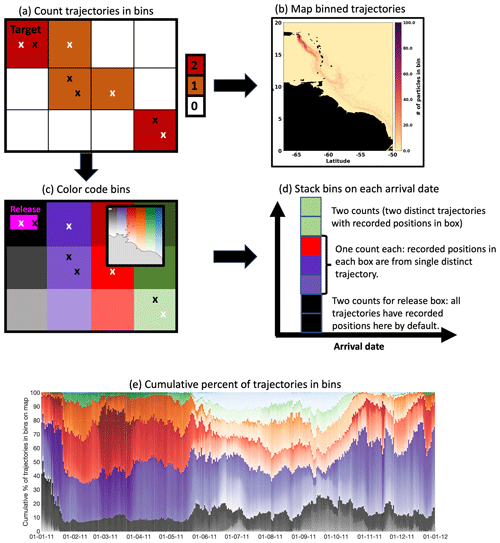
Figure B1 Schematic demonstrating the method used to generate Fig. B2. (a) Example positions of a trajectory for two particles (one black and one white). The “Release” bin corresponds to the release site from which particles are backtracked. Positions within 0.2°×0.2° bins are counted and mapped, as shown in panel (b). (c) Bins are now color-coded by their location (actual example in the inset map). A change in color represents a meridional position change, while a change in shading corresponds to a latitudinal position change. (b) Example of position counting in each bin. (d) Example schematic of how the time series is generated. For each arrival date, bins are stacked by the number of particles in each bin (scaled by the number of bins with recorded particles). (e) Actual example of the time series. The colored bins stacked on top of each day in the x axis represent the pathway that the waters came from. The inset map in panel (c) shows the color-coded bins to identify pathways. For a detailed description, refer to Seijo-Ellis et al. (2023).

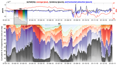
Figure B2 (a) Time series of SSS (red; right vertical axis), horizontal SSS advection (blue; left vertical axis), and SSS tendency (black; left vertical axis) within the VIB during 2010. (b) Map with color-coded bins used to identify the path of trajectories is shown in panel (c). A change in bin color denotes a change in longitude, and a change in shade (from light to dark) represents a change in latitude (from south to north). (c) Time series of cumulative percent of the trajectories in each bin; for each particle release date (i.e., for each arrival date into the region of interest as we are backtracking), we stacked bins following the description in Seijo-Ellis et al. (2023). Bin colors indicate bin locations and correspond to the color distribution in panel (b). As an example, a high cumulative percent of trajectories in light-colored bins (red through blue) indicates that particles arrived to the VIB from the southwest along a path close the coast of South America.