P3D-BRNS v1.0.0: a three-dimensional, multiphase, multicomponent, pore-scale reactive transport modelling package for simulating biogeochemical processes in subsurface environments

The porous microenvironment of soil offers various environmental functions which are governed by physical and reactive processes. Understanding reactive transport processes in porous media is essential for many natural systems (soils, aquifers, aquatic sediments or subsurface reservoirs) or technological processes (water treatment or ceramic and fuel cell technologies). In particular, in the vadose zone of the terrestrial subsurface the spatially and temporally varying saturation of the aqueous and the gas phase leads to systems that involve complex flow and transport processes as well as reactive transformations of chemical compounds in the porous material. To describe these interacting processes and their dynamics at the pore scale requires a well-suited modelling framework accounting for the proper description of all relevant processes at a high spatial resolution. Here we present P3D-BRNS as a new open-source modelling toolbox harnessing the core libraries of OpenFOAM and coupled externally to the Biogeochemical Reaction Network Simulator (BRNS). The native OpenFOAM volume-of-fluid solver is extended to have an improved representation of the fluid–fluid interface. The solvers are further developed to couple the reaction module which can be tailored for a specific reactive transport simulation. P3D-RBNS is benchmarked against three different flow and reactive transport processes: (1) fluid–fluid configuration in a capillary corner, (2) mass transfer across the fluid–fluid interface and (3) microbial growth with a high degree of accuracy. Our model allows for simulation of the spatio-temporal distribution of all biochemical species in the porous structure (obtained from μ-CT images), for conditions that are commonly found in the laboratory and environmental systems. With our coupled computational model, we provide a reliable and efficient tool for simulating multiphase, reactive transport in porous media.

1 Introduction

Subsurface environments (soils, aquifers, aqueous sediments) are (typically) porous media that host a multitude of biogeochemical processes and interactions and provide different versatile ecosystem functions (e.g. C sequestration; compound degradation; nutrient retention; provision of food, fibres and fuel; habitat for organisms; and water retention and purification; Baveye et al., 2016). These processes are controlled by various biological (e.g. microbial abundance and activity), chemical (e.g. distribution of dissolved and volatile species, mineral composition, and surface properties of the solid matrix) and physical (e.g. porous structure and permeability, water saturation) properties of the system. These features create a complex web of interactions, the magnitude and effectiveness of which change dynamically in space and time (Graham et al., 2014). Microbial communities, for example, and their metabolic capacity are considered to be directly related to energy and matter fluxes (Thullner et al., 2007), which are, in turn, governed by pore arrangements and their connectivity. Along with other environmental factors, this can also modify various properties of the porous media (e.g. by biomass accumulation on pore walls (Thullner, 2010) or mineral dissolution or precipitation (Meakin and Tartakovsky, 2009), which in turn are altering the conditions for biogeochemical processes, too.

In soils (or more generally the vadose zone), the dynamically varying distribution of the aqueous and gaseous phase leads to specifically complex and variable constraints for biogeochemical processes. In the past, obtaining (bio)chemical and microbiological information at the pore level was neither economically nor logistically a feasible option (Baveye et al., 2014). Also for the sake of applicability, traditionally, researchers had more tendency to look for Darcy-scale solutions to tackle environmental issues (White and Brantley, 2003). The Darcy-scale view (experimental, theoretical or a mixture of both) serves the purpose of practical applicability well (White and Brantley, 2003), but, for example, in the context of microbially mediated degradation processes in the vadose zone, it fails to provide insights on the driving mechanisms, as it overlooks important contributing factors, such as the tortuous porous structure/pathways open to the transport of (bio)geochemical species and the non-uniform distribution of water and air phases, as well as the nonlinear dependency between changes of the local nutrient and biomass concentrations and the bulk concentrations of (bio)geochemical species. Evidence at the microscopic level has shown that biological activity and evolution are more locally organized (Kuzyakov and Blagodatskaya, 2015) where Darcy-scale studies lead to loss of crucial information. This has motivated the development of sophisticated physics-based models implementing all aspects of hydrological, geochemical and biological processes involved in microbial growth and evolution.

Reactive transport models (RTMs) are a class of mathematical models that have been applied extensively to study biogeochemical systems for about four decades (Parkhurst and Appelo, 1999; Thullner et al., 2005; Thullner and Regnier, 2019; Meile and Scheibe, 2019). There is a long list of principal factors and mechanisms governing biogeochemical reactions at the pore scale. Numerically, these processes can be defined and solved either by fully (global) implicit approaches or by separating and solving different components one at a time. For the Darcy scale, a wide range of reactive transport models exist which allow for the simulation of biogeochemical processes (Steefel et al., 2015b). In turn, at the pore scale, models combining the simulation of flow, transport and reactive (biogeochemical) processes are scarce, and existing model developments are often driven by specific research questions and/or are subject to severe simplifications in the description of the pore space (Golparvar et al., 2021). Integrated models explicitly capturing the structural properties of the soil at the pore scale, the resulting multiphase flow and multispecies reactive transport simultaneously are hardly available (Tian and Wang, 2019).

Recently, new frontiers of pore-scale RTMs are emerging with the advances in computational power as well as with huge improvements in imaging techniques. The latter includes, for example, the static and dynamic scanning of porous structure as well as of fluids' distribution (Schlüter et al., 2019) or the detection of bacterial distributions in soil using the catalysed reporter deposition with fluorescence in situ hybridization (CARD-FISH) technique (Schmidt et al., 2015). Direct numerical models (DNMs) are becoming the nexus of the next generation of RTMs as they represent the porous structure in a fully explicit manner (directly obtained from soil samples, digitized and fed into RTMs) in addition to offering a more flexible coupling of different components of reactive transport models (Baveye et al., 2018; Raeini et al., 2012; Li et al., 2010; Yan et al., 2016). Another advantage of using DNMs is that they offer a great deal of flexibility in considering settings and conditions that are experimentally impossible to impose (Tian and Wang, 2019).

In this work, we introduce the pore-scale RTM package P3D-BRNS explicitly involving the structure and topology of the pore space, the co-existence/co-flow of both the aqueous and the gaseous phase, the advective–diffusive transport of species in each phase, and an arbitrary set of reactive processes controlled by kinetic rate laws or thermodynamic constraints. The fluid flow field is updated via solving the Navier–Stokes (NS) equations (Patankar and Spalding, 1972). The volume-of-fluid (VOF) approach is adopted to account for different phase distribution (Hirt and Nichols, 1981). The transport of chemical species is considered via solving the advection–diffusion–reaction equation (ADRE), where the concentration jump for soluble/volatile compounds across the fluid–fluid interface is modelled via the continuous species transfer (CST) method (Haroun et al., 2010). Reactive processes are defined and simulated externally via coupling the flow and transport model to the BRNS (Biogeochemical Reactions Network Solver) package (Regnier et al., 2002; Aguilera et al., 2005). The model structure is introduced, and the model performance is shown and compared with analytical counterparts. The model capabilities are depicted for a fully three-dimensional case.

2 Mathematical formulation

The entire numerical domain (Ω) can be decomposed to two main sub-regions: solid space (Ω_S) and void space (Ω_ϑ). The void space is further divided into aqueous phase (Ω_ϑ,aq) and gaseous phase (Ω_ϑ,gs), which are partitioned by the fluid–fluid interface (Ω_I). The overall domain is bounded externally between inlet (Ω_in) and outlet (Ω_out) boundaries, which allow for the inflow/outflow of different phases and chemical species, as well as no-flux boundaries resembling physical walls, where nothing is allowed to leave or enter the domain (Ω_wall). The domain is limited internally by no-flow boundaries where solid space and void space intersect (i.e. solid surface,${\mathrm{\Omega }}_{\mathit{\vartheta }}\bigcap {\mathrm{\Omega }}_{\mathrm{S}}={\mathrm{\Omega }}_{\mathrm{wall}})$.

2.1 Fluid flow: governing equations

Evolution of a single/multi-phase, isothermal, incompressible, immiscible fluid(s) can be expressed by basic conservation principles. These can be formulated into a single-field formalism (Hirt and Nichols, 1981):

$$\begin{array}{}\text{(1)}& {\displaystyle }\mathrm{\nabla }\cdot \mathbf{u}=\mathrm{0}\text{in}{\mathrm{\Omega }}_{\mathit{\vartheta }}\text{(2)}& {\displaystyle }\mathit{\rho }\left({\displaystyle \frac{\partial \mathbf{u}}{\partial t}}+\mathbf{u}\cdot \mathrm{\nabla }\mathbf{u}\right)=-\mathrm{\nabla }P+\mathrm{\nabla }\cdot \mathit{\tau }+\mathit{\rho }g+F_{\mathit{\sigma }}\text{in}{\mathrm{\Omega }}_{\mathit{\vartheta }},\end{array}$$

where u is the vector of velocity field; ρ is the fluid density; P is the pressure; g is the gravitational vector; and τ is the stress tensor, which can be defined as $\mathit{\tau }=\mathrm{2}\mathit{\mu }S=\mathrm{2}\mathit{\mu }\left(\mathrm{0.5}\left[\left(\mathrm{\nabla }\mathbf{u}\right)+{\left(\mathrm{\nabla }\mathbf{u}\right)}^T\right]\right)$, with μ as the fluid viscosity. F_σ denotes the interfacial tension force, which is only nonzero when two or more phases (excluding solid) are available. It is safe to use the incompressible form of the Navier–Stokes equation for low Mach and Reynolds numbers.

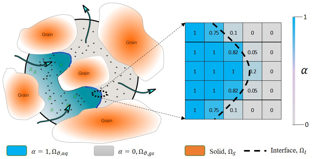
Figure 1 Illustration of a porous medium at the pore scale with one fluid invading the other (on the left). Mathematical representation of the phase saturation in the computational cells around the interface (on the right). The dashed line shows the actual location of the interface while values in each cells show the amount of water saturation relevant to topology of the dashed line. Black dots represent volatile compounds able to cross the fluid–fluid interface, and green dots represent non-volatile compounds restricted to the transport in the aqueous phase.

In the case of simultaneous flow of two different phases, their locations and distribution are represented via introducing an indicator function, α, taking values within the range [0, 1]. The first continuous fluid is marked as α=1, and the second fluid is denoted as $\mathit{\beta }=\mathrm{1}-\mathit{\alpha }$, and for the transition from one fluid to the other (i.e. the interface, Ω_I), α varies between 0 and 1. Fluid density and viscosity in each grid cell is then calculated from a linear interpolation of this indicator function:

$$\begin{array}{}\text{(3)}& {\displaystyle }\mathit{\rho }=\mathit{\alpha }{\mathit{\rho }}_{\mathrm{1}}+\left(\mathrm{1}-\mathit{\alpha }\right){\mathit{\rho }}_{\mathrm{2}}\text{in}{\mathrm{\Omega }}_{\mathit{\vartheta }}\text{(4)}& {\displaystyle }\mathit{\mu }=\mathit{\alpha }{\mathit{\mu }}_{\mathrm{1}}+\left(\mathrm{1}-\mathit{\alpha }\right){\mathit{\mu }}_{\mathrm{2}}\text{in}{\mathrm{\Omega }}_{\mathit{\vartheta }}.\end{array}$$

A mass conservative boundary condition at the fluid–fluid interface is written as

$$\begin{array}{}\text{(5)}& [{\mathit{\rho }}_i\left({\mathbf{u}}_i-w\right)\cdot n_{{\mathrm{\Omega }}_{\mathrm{I}}}]=\mathrm{0}\text{in}{\mathrm{\Omega }}_{\mathrm{I}},\end{array}$$

with ρ_i as the density of ith fluid, u_i as the velocity of ith fluid, w as the velocity of the interface, ${\mathrm{n}}_{{\mathrm{\Omega }}_{\mathrm{I}}}$ as the normal vector to the interface (Ω_I) pointing from the invading phase to the displaced one and the brackets showing the jump condition at the interface. Individual velocities, u_i, and the interface velocity w, are not directly calculated but furthermore averaged to derive the global mass conservation equation that is used for numerical discretization (for full derivation, consult Graveleau et al., 2017).

In the context of the finite-volume method (FVM), discretization of the physical domain produces a finite subset of discrete volumes (taking the shape of a polyhedral). The key implication of the volume-of-fluid method is to define and solve for global variables, rather than having one equation for each variable in each phase. Hence, the idea is to transform the integro-differential equations into their global versions by averaging them over each cell volume (Whitaker, 2013). For multiphase systems, after a few steps of linearization and approximation (see Hirt and Nichols, 1981, for a detailed derivation), the volume-of-fluid formulation of the momentum equation (Eq. 2) is obtained as

$$\begin{array}{}\text{(6)}& \begin{array}{rl}\mathit{\rho }& \left({\displaystyle \frac{\partial \stackrel{\mathrm{‾}}{\mathbf{u}}}{\partial t}}+\stackrel{\mathrm{‾}}{\mathbf{u}}\cdot \mathrm{\nabla }\stackrel{\mathrm{‾}}{\mathbf{u}}\right)=-\mathrm{\nabla }P+\mathrm{\nabla }\cdot \mathit{\mu }\left(\mathrm{\nabla }\stackrel{\mathrm{‾}}{\mathbf{u}}+{\left(\mathrm{\nabla }\stackrel{\mathrm{‾}}{\mathbf{u}}\right)}^t\right)\\ & +\mathit{\rho }g+F_{\mathit{\sigma }}\text{in}{\mathrm{\Omega }}_{\mathit{\vartheta }},\end{array}\end{array}$$

with having $\stackrel{\mathrm{‾}}{\mathbf{u}}$ as the global averaged velocity vector. For the sake of simplicity, we drop the “average” notation from the global velocity vector (i.e. will refer to $\stackrel{\mathrm{‾}}{\mathbf{u}}$ as u), for the rest of this paper. The pressure gradients (and Reynolds numbers) considered in our simulations are in the range that render changes in the gas compressibility negligible.

Since we are dealing with only two fluids, index i in u_i takes only two values; α and β – one for each phase. A global, mass conservative, advection equation is used to describe the evolution of the indicator function:

$$\begin{array}{}\text{(7)}& {\displaystyle \frac{\partial \mathit{\alpha }}{\partial t}}+\mathrm{\nabla }\cdot \left(\mathit{\alpha }\mathbf{u}\right)+\mathrm{\nabla }\cdot \left(\mathit{\alpha }\left(\mathrm{1}-\mathit{\alpha }\right){\mathbf{u}}_{\mathrm{c}}\right)=\mathrm{0}\text{in}{\mathrm{\Omega }}_{\mathit{\vartheta }},\end{array}$$

where α indicates the volume fraction of phase 1, and $u_{\mathrm{c}}=u_{\mathit{\alpha }}-u_{\mathit{\beta }}$ is the vector of the compressive velocity, with u_α,β as the velocity vector of phase α and β right on the edge of the interface (detailed explanation on deriving Eq. 7 can be found in the Supplement). It is derived from the mass conservation equation written for phase α, which computationally helps with maintaining stiffness/sharpness of the interface. Sharpening the interface means having the interface span fewer computational grids. u_c is the vector of compressive velocity on each face of all computational grids. Since we do not solve for the velocity field of each phase individually, a direct calculation of u_c is not possible. However, we can rather take an indirect approach for computing u_c as follows:

$$\begin{array}{}\text{(8)}& {\mathbf{u}}_{\mathrm{c}}=min\left(c_{\mathit{\alpha }}\left|\mathbf{u}\right|,max\left(\left|\mathbf{u}\right|\right)\right){\displaystyle \frac{\mathrm{\nabla }\mathit{\alpha }}{\left|\mathrm{\nabla }\mathit{\alpha }\right|}}\text{in}{\mathrm{\Omega }}_{\mathrm{I}}.\end{array}$$

In Eq. (8), c_α is a compression coefficient providing some level of control over how wide the interface spans. The max function operates on the magnitude of unit velocity vector calculated on all the faces of a computational grid. To counteract the numerical diffusion and avoid the spread of interface over several computational grids, values of c_α>1 provide an enhanced/sharper interface, whereas a value of c_α=0 gives no compression of the interface (Graveleau et al., 2017). In simulation scenarios introduced in this paper, c_α has been assigned the value of 1, unless stated otherwise.

To calculate the interfacial tension force, F_σ, Brackbill et al. (1992) have introduced a continuum surface force (CSF) which requires computation of the curvature of the interface:

$$\begin{array}{}\text{(9)}& \mathit{\kappa }=\mathrm{\nabla }.n_{{\mathrm{\Omega }}_{\mathrm{I}}}\text{in}{\mathrm{\Omega }}_{\mathrm{I}},\end{array}$$

with having κ as the mean interface curvature in each computational grid and $n_{{\mathrm{\Omega }}_{\mathrm{I}}}$ as the interface unit normal vector, defined as

$$\begin{array}{}\text{(10)}& n_{{\mathrm{\Omega }}_{\mathrm{I}}}={\displaystyle \frac{\mathrm{\nabla }\mathit{\alpha }}{\left|\mathrm{\nabla }\mathit{\alpha }\right|}}\text{in}{\mathrm{\Omega }}_{\mathrm{I}}.\end{array}$$

Given the curvature, the interfacial tension force can be approximated as

$$\begin{array}{}\text{(11)}& {\mathrm{F}}_{\mathit{\sigma }}=\mathit{\sigma }\mathit{\kappa }\mathrm{\nabla }\mathit{\alpha }\text{in}{\mathrm{\Omega }}_{\mathrm{I}},\end{array}$$

where σ is the surface tension between two fluids (derivation of this approximation can be found in Brackbill et al., 1992).

2.2 Reactive transport: governing equations

Concentrations of mobile species are affected by advection (i.e. transport with the moving fluid), molecular diffusion and reactive transformation. Also, in the case of having two fluids simultaneously in the system, different species can cross the fluid–fluid interface, causing local fluctuations in concentration values. In general to account for all the changes in species concentrations, the ADRE for biogeochemical reactive components can be written as

$$\begin{array}{}\text{(12)}& {\displaystyle \frac{\partial C_i}{\partial t}}+\mathrm{\nabla }\cdot \left(C_i\mathbf{u}\right)=-\mathrm{\nabla }\cdot \left(J_{\mathrm{d},i}+J_{\mathrm{m},i}\right)+R_i\text{in}{\mathrm{\Omega }}_{\mathit{\vartheta }},\end{array}$$

where J_d,i is the molecular diffusive flux of component i, J_m,i is the mass flux of component i due to mass transfer across the fluid–fluid interface and R_i accounts for the changes in concentration of component i due to reactions. Molecular diffusion follows Fick's law:

$$\begin{array}{}\text{(13)}& J_{\mathrm{d},i}=-D_i\mathrm{\nabla }\left(C_i\right)\text{in}{\mathrm{\Omega }}_{\mathit{\vartheta }},\end{array}$$

where D_i is the diffusion coefficient of species i. At the interface, the assumption of thermodynamic equilibrium implies equality of chemical potentials. Given the condition that liquid concentration of component i is proportional to the partial pressure of the species in the secondary phase (e.g. gas, oil or minerals), a partitioning relationship such as Raoult or Henry's law (Danckwerts and Lannus, 1970) can be established to relate species concentrations on both sides of the interface:

$$\begin{array}{}\text{(14)}& C_{i,\mathit{\beta }}=H_i{C}_{i,\mathit{\alpha }}\text{in}{\mathrm{\Omega }}_{\mathrm{I}},\end{array}$$

with C_i,α as the concentration of species i in phase α, H_i as Henry's constant of species i and C_i,β as the concentration of species i in phase β. Depending on if a given compound's concentration in the aqueous phase or the gaseous phase is multiplied by Henry's coefficient (Eq. 14), the definition of Henry's constant switches between the solubility or volatility for that compound (i.e. $H_i^{\mathrm{soluility}}=\mathrm{1}/H_i^{\mathrm{volatility}})$ (Sander, 2015). Unless otherwise stated, the volatility concept of Henry's law is adopted in order to define the concentration relationship of a given compound across the fluid–fluid interface (Eq. 14). The concentration field around the fluid–fluid interface (where ∇α≠0) at equilibrium, for any values of H≠1, is discontinuous, which imposes the additional flux, J_m,i, to satisfy the concentration jump across the interface. Hence the mass transfer flux, J_m,i, can be derived within the VOF framework (i.e. CST) as follows (Haroun et al., 2010):

$$\begin{array}{}\text{(15)}& J_{\mathrm{m},i}=-D_i{\displaystyle \frac{\mathrm{1}-H_i}{\mathit{\alpha }+\left(\mathrm{1}-\mathit{\alpha }\right)H_i}}{C}_i\mathrm{\nabla }\mathit{\alpha }\text{in}{\mathrm{\Omega }}_{\mathit{\vartheta }}.\end{array}$$

It is noteworthy that few assumptions and volume averaging methods are implemented to derive Eq. (15); readers are encouraged to check the references for more details. The diffusion coefficient is calculated from harmonic interpolation:

$$\begin{array}{}\text{(16)}& D_i={\displaystyle \frac{\mathrm{1}}{\frac{\mathit{\alpha }}{D_{i,A}}+\frac{\mathrm{1}-\mathit{\alpha }}{D_{i,B}}}}\text{in}{\mathrm{\Omega }}_{\mathit{\vartheta }},\end{array}$$

where $D_{i,\mathit{\alpha }-\mathit{\beta }}$ is the diffusion coefficient of species i in phase α and β respectively.

Simulated reactions include kinetically as well as thermodynamically constrained reactions. For a kinetically constrained reaction j, the reaction rate $r_j=f(C_{\mathrm{1}},\mathrm{\dots },C_n)$ is needed, while for a thermodynamically constrained reaction k, the equilibrium conditions defined by a law of mass action $M_k=f(C_{\mathrm{1}},\mathrm{\dots },C_n)$ are needed, with M_k as the equilibrium constant. These equations can be of arbitrary form, and the resulting reaction network defines the term R_i in Eq. (12) (Aguilera et al., 2005; Regnier et al., 2002). For immobile species, concentration changes are only due to reactive processes.

2.3 Boundary conditions (BCs)

There are various types of boundary conditions, corresponding to the real physical conditions, most of which can be derived from two basic types:

• the Dirichlet boundary (fixed value), which relates the value of a variable at a given geometric location to a constant value, for example, C_i=1M in Ω_in, meaning a constant 1 molar concentration of component i at the boundary,

• the von Neumann boundary (fixed gradient), which provides the value of a variable's gradient at the face of the boundary cell, for example, ${\partial }_n\mathbf{p}=\mathrm{0}$ in Ω_wall, giving a zero pressure gradient on the wall.

In general, our model can apply any of these basic boundary conditions to any scalar or vector variables such as pressure, velocity/flux and concentration of volume-of-fluid fields, but one needs to ensure that the imposed BC(s) are both compatible and that they reflect the correct physical boundary conditions. For example, for velocity/flux–pressure coupling, a Dirichlet (i.e. constant) boundary for flux at the inlet can be coupled with either (1) fixed discharge velocity/flux and zero-gradient (i.e. von Neumann) pressure at both the inlet and outlet, (2) a constant pressure head at the inlet and atmospheric pressure at the outlet with zero-gradient velocity/flux at both ends, or (3) fixed values of pressure and velocity/flux at one end and zero gradient at the other end. In the beginning of Sect. 2, the typical composition and configuration of an arbitrary computational domain are described. Inlet, outlet and impermeable boundaries are amongst the most common types that one might face. Inlet BC means for the direction of fluid flux to be pointing inwards (i.e. into the domain), while for the outlet, the direction of the flux should be outwards. Also for the impermeable wall, zero-orthogonal fluxes need to be satisfied. Either Dirichlet, von Neumann or a mixture of both can be used at a particular boundary. Mathematical translation and implementation of these boundaries are provided in the next section. Time-dependent BCs (e.g. cyclic or seasonal water/species influx) are also readily available to be applied but have never been used in this work. Unless otherwise stated, boundary conditions that have been imposed on each section of the computational domain are described as follows.

At impermeable boundaries (Ω_wall). The physical wall implies no flux perpendicular to the normal vector to its surface. No-slip BC is an appropriate BC for the velocity field on the wall. In general, they can all be written as

$$\begin{array}{}\text{(17)}& \begin{array}{rl}& {\partial }_n{\mathbf{C}}_i=\mathrm{0},{\mathbf{u}}_{x,y,z}=\mathrm{0},{\partial }_n\mathbf{p}=\mathrm{0},\\ & {\partial }_n\mathit{\alpha }=\mathrm{0}\text{in}{\mathrm{\Omega }}_{\mathrm{wall}}.\end{array}\end{array}$$

For the velocity field, on the wall, a slip boundary condition is also available to be applied.

At inlet–outlet boundaries (Ω_inΩ_out). The concentrations of reactants, products and inert tracers are set to fixed values at inlet, while they are allowed to leave the domain at the outlet with zero-gradient boundary conditions. A constant flow rate with zero-pressure gradient is applied at the inlet, and an atmospheric pressure (fixed value) with zero velocity gradient is set at outlet. Also, in the case of two-phase flow, the invading phase is set to enter from the inlet at a fixed value and exits from the outlet with zero-gradient BCs. Mathematically, they can be expressed as

$$\begin{array}{}\text{(18)}& {\mathrm{C}}_i\ge \mathrm{0},\mathbf{u}=\mathrm{const}{\partial }_n\mathbf{p}=\mathrm{0},\mathit{\alpha }=\mathrm{const}.\text{in}{\mathrm{\Omega }}_{\mathrm{in}}\end{array}$$

together with

$$\begin{array}{}\text{(19)}& {\partial }_n{\mathbf{C}}_i=\mathrm{0},{\partial }_n{\mathbf{u}}_{\mathrm{n}}=\mathrm{0},\mathbf{p}=\mathrm{0},{\partial }_n\mathit{\alpha }=\mathrm{0}\mathrm{in}{\mathrm{\Omega }}_{\mathrm{out}},\end{array}$$

with u_n as the normal velocity vector. While we have mostly applied Eqs. (18) and (19) for designing an inlet–outlet duo, other formats, such as defining a pressure head (and zero-gradient velocity) on the inlet in combination with either constant exit pressure or constant discharge rate, are readily available to implement as well.

At the fluid–fluid–solid contact line $\left({\mathrm{\Omega }}_{{\mathrm{l}}^{\mathrm{3}}}\right)$. At the fluid–fluid–solid contact line, in the case of no interactions or no reaction of any chemical species with the solid, the boundary condition at the triple point is derived to be

$$\begin{array}{}\text{(20)}& \mathrm{\nabla }{C}_i\cdot {\mathbf{n}}_{\mathbf{s}}={\displaystyle \frac{H_i-\mathrm{1}}{\mathit{\alpha }{H}_i+\left(\mathrm{1}-\mathit{\alpha }\right)}}{C}_i\mathrm{\nabla }\mathit{\alpha }\cdot {\mathbf{n}}_{\mathrm{s}}\text{in}{\mathrm{\Omega }}_{\mathrm{I}},\end{array}$$

with n_s as the normal vector to the solid surface (Graveleau et al., 2017). Also, the concept of contact angle is applied by making the following modification to the interface normal vector:

$$\begin{array}{}\text{(21)}& {\mathrm{n}}_{{\mathrm{\Omega }}_{{\mathrm{l}}^{\mathrm{3}}}}=\cos \mathit{\theta }{\mathbf{n}}_{\mathrm{s}}+\sin \mathit{\theta }{\mathbf{t}}_{\mathrm{s}}\text{in}{\mathrm{\Omega }}_{l^{\mathrm{3}}},\end{array}$$

where n_s is the normal vector, and t_s is the tangential vector to the solid surface (Brackbill et al., 1992). At the triple point, i.e. fluid–fluid–solid interface, ${\mathrm{n}}_{{\mathrm{\Omega }}_{{\mathrm{l}}^{\mathrm{3}}}}$is used for normal vector to the interface. CSF, though, has been reportedly generating non-physical spurious currents (Scardovelli and Zaleski, 1999). For this, many have tried to eliminate/mitigate this issue by explicit representation of the interface either via using the geometric VOF method (Popinet, 2009) or coupled level-set (LS) VOF functions (Albadawi et al., 2013). Geometric VOF is quite suitable for structured grids, but for porous structures with highly unstructured grids, the calculations can become quite complicated. Alternatively, Raeini et al. (2012) suggested filtering the capillary forces parallel to the interface, which can significantly reduce the non-physical velocities. In short, the modifications they proposed and which are used here are (1) smoothing the indicator function to have a better measure of the interface curvature, (2) sharpening the indicator function for computation of the interfacial tension force, (3) filtering the capillary pressure force parallel to the interface and (4) filtering capillary fluxes based on the capillary pressure gradient (for a full description of each point, please consult with Raeini et al., 2012). The correction introduced for filtering capillary forces helps with eliminating some of the parasitic velocities parallel to the interface. To sum up what has been presented so far, we integrated (a) the original interFoam solver from the OpenFOAM library that only solves for the advection–diffusion transport of two phase flow with (b) the improved-interface-resolver library from Raeini et al. (2012) and (c) added a scalar transport solver on top of them. Finally, the full-scale advection–diffusion–reaction model of the biogeochemical species is attained by coupling this to an external reaction network solver, which is explained in Sect. 2.4.

2.4 Numerical formulation

The mass conservation (Eq. 1), momentum (NS – Eq. 2) and indicator function (Eq. 7) equations are all implemented within the open-source computational fluid dynamics (CFD) package, OpenFOAM (Greenshields, 2015). OpenFOAM utilizes the finite-volume methodology (FVM), a common choice for CFD problems as FVM works only with conservative flux evaluation at each computational cell's boundaries, making it robust in handling nonlinear transport problems. Also all the differential equations mentioned before are first written in their integral form over each cell volume and then converted to the surface summations using Green's theorem.

The original two-phase (VOF) flow solver, i.e. interFoam, is modified to construct our biogeochemical reactive transport package. The momentum equation (Eq. 2) is linearized in a semi-discrete form as

$$\begin{array}{}\text{(22)}& A_{\mathrm{d}}\mathbf{u}=\mathbf{H}\left(\mathbf{u}\right)-\mathrm{\nabla }P+\mathbf{F},\end{array}$$

where A_d holds the diagonal elements of the coefficient matrix, H(u) contains off-diagonal elements of the coefficient matrix including all source terms and F entails any body forces (interfacial tension force only in this case). Temporal discretization is handled via the first-order Euler method, while spatial discretization is managed via second-order finite-volume schemes. Convection terms of the momentum equation and indicator function (Eq. 7) are computed using a bounded self-filtered central differencing (SFCD) scheme (based on Gauss's theorem). Rearranging Eq. (22) for velocity and imposing the continuity equation (Eq. 1), the following linear pressure equation can be obtained:

$$\begin{array}{}\text{(23)}& \sum _f{\displaystyle \frac{S_f}{\langle A_f\rangle }}{\mathrm{\nabla }}_f^{\perp }P=\sum _f\left(\langle {\displaystyle \frac{H\left(u\right)}{A_{\mathrm{d}}}}{\rangle }_f\cdot \left|S_f\right|+{\displaystyle \frac{{\mathit{\phi }}_{\mathrm{F},f}}{\langle A_{\mathrm{d}}{\rangle }_f}}\right).\end{array}$$

S_f in Eq. (23) denotes the outward area vector of face f, the notation ${\mathrm{\nabla }}_f^{\perp }$ shows face normal gradients calculated right on the face centres, 〈〉_f shows the interpolated values of a face-centred parameter from its cell-centred counterpart and φ_F,f is the interfacial force flux term.

The velocity–pressure coupling of Eqs. (1) and (2) is solved using Pressure Implicit with Splitting of Operators (PISO) (Issa, 1986). PISO embodies a predictor–corrector strategy to simultaneously update pressure and velocity within each time step. The resultant system of equations is solved on the cell faces and then interpolated back to calculate velocities and pressure at the cell centres. The coupling of the indicator function (Eq. 7) and momentum equation is explicitly defined and solved right after the PISO step is finished. Within the same time step, transport and reaction of different species are then solved sequentially – using a sequential non-iterative algorithm (Steefel et al., 2015a; Steefel and MacQuarrie, 1996). Time step size is controlled by introducing a Courant number. Time is discretized using either Euler or Crank–Nicolson methods, and spatial discretization is performed using the van Leer second-order total variation diminishing scheme (TVD) (van Leer, 1979).

The reaction network is built separately and externally solved within the BRNS package – which employs first-order Taylor series expansion terms and uses the Newton–Raphson method to iteratively solve the system of linear equations (Regnier et al., 2002). BRNS utilizes MAPLE programming language to construct the Jacobian matrix (which contains the partial derivatives of unknown parameters, i.e. concentrations) and other problem-related data such as rate parameters and translating them to a FORTRAN package. The FORTRAN code is then compiled to generate shared objects (*.so file) that can be dynamically called later from the transport solver (Centler et al., 2010). The significance of having dynamically shared object files is more apparent when running computationally demanding cases/scenarios while decomposing and running the application in parallel. BRNS is invoked once the new concentrations are computed from the transport solver. The updated concentrations from the BRNS library (i.e. updating concentrations from redox reactions) are then fed back into the transport solver before moving to the next time step. This process repeats until the final time is reached. This coupling scheme has been successfully used for other RTM approaches before (Centler et al., 2010; Gharasoo et al., 2012; Nick et al., 2013). As the reactions are localized, the reaction solver is modular, and OpenFOAM inherently provides parallelized simulations (via domain decomposition). The P3D-BRNS can easily be used to model larger systems. To achieve higher performance, it is recommended to utilize physical cores rather than hyper-threading. The parallelization of our model strengthens its scalability in the sense of the size (pore scale or Darcy scale) of the simulated system. However, in terms of upscaling (e.g. from the pore scale to the Darcy scale), an intermediate step would be required depending on the complexity of the processes that are involved and on the size of the domain.

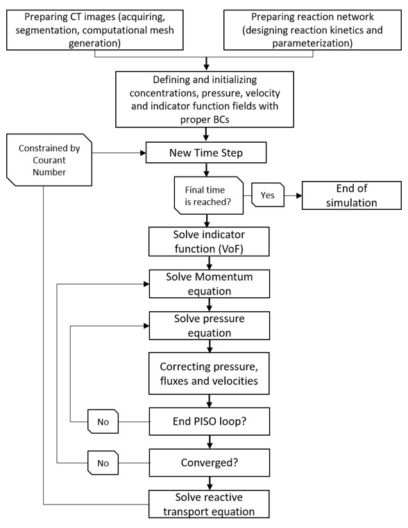
Figure 2 Full solution procedure to simulate a reactive transport process at its fullest complexity.

Prior to run simulations, the physical settings of the domain are required to be specified; i.e. the physical geometry of the pore space with proper boundaries and the meshing scheme should be designed. OpenFOAM provides a basic utility for defining boundaries as well as mesh generation which are translatable by the OpenFOAM engine. Any other meshing software/freeware can be freely used as long as an OpenFOAM-compatible format for the meshed file can be created. The overall workflow required to build and run a case/scenario is summarized in Fig. 2.

3 Model performance

The presented reactive transport model is designed (1) to capture real-world pore structures in up to three dimensions, (2) to explicitly simulate the transient distribution of a gas and a liquid phase within the entire pore space, and (3) to simulate a full set of advection–diffusion–reaction mechanisms. Capturing the correct curvature of the interface depends heavily on the grid resolution. For a fixed velocity magnitude, a higher grid resolution enforces a shorter time step size (from Courant number) for the numerical simulations to converge. Also, to validate different features of the model various, simplified scenarios were used which allow the use of analytical expressions as reference for the numerical results. Here we show three representative test scenarios addressing different features of the model (two-phase flow, mass transfer across the fluid–fluid interface and reactive transport) individually. Subsequently, the model capabilities are depicted in a final biodegradation scenario, making use of the various model features simultaneously.

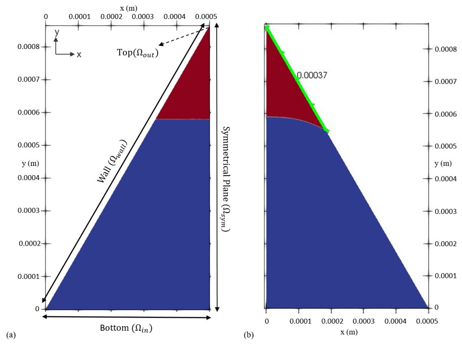
Figure 3 Initial condition (a) versus final arrangement (b) of the two phases in the fluid configuration scenario. The blue colour indicates the non-wetting phase, and the red colour shows the wetting phase respectively. The dashed arrow shows the location of the outlet, while the solid-line arrows depict the extent of others boundaries. Once equilibrium is reached (b), the curvature of the interface corresponds to the force balance between pressure difference across the interface and the surface tension which can be used to verify the model's sanity. The distance of the contact point (i.e. the point/line where all three phases – water, air and solid – meet) from the corner vertex (highlighted as green) also provides another measure for checking the accuracy of the numerical model.

3.1 Fluid configurations

In order to test our model's performance in simulating two-phase flow, we have zoomed into a two-dimensional porous structure and isolated only one single corner, taking the shape of an equilateral triangle. A triangulated mesh is adopted that naturally conforms to the overall shape of the domain. Initially, two immiscible fluids (one wetting and one non-wetting, for example, water and air) are placed in such a way that their interface forms a straight line (Fig. 3a). The side length of the triangle is 1 mm with a mesh size of 1 µm. Under thermodynamic equilibrium conditions, the force exerted by the pressure difference between two phases is countered by the interfacial tension force. This, along with the contact angle of the non-wetting phase at the wall surface in presence of the wetting phase (e.g. water), determines the topology of the fluid–fluid interface. For a given corner half-angle, the distance that the wetting phase spreads over the solid surface from the corner vertices (the highlighted section in green in Fig. 3b), b, can be calculated as

$$\begin{array}{}\text{(24)}& b=r{\displaystyle \frac{\cos (\mathit{\theta }+\mathit{\beta })}{\sin \left(\mathit{\beta }\right)}},\end{array}$$

with r as the radius of the interface's curvature, θ as the contact angle and β as the corner half-angle (Blunt, 2017). In order to reach thermodynamic equilibrium, we performed transient, two-phase flow simulations to compute velocity, pressure and indicator function fields until the triple contact line $\left({\mathrm{\Omega }}_{{\mathrm{l}}^{\mathrm{3}}}\right)$ is static. For this, we first divided the equilateral triangle in half, as the problem is symmetrical along the height of the triangle. The symmetrical plane implies that there is no gradient (of any scalar or vector field) perpendicular to its surface, while the tangential components (of all fields) remain the same. To find the fluid configuration at equilibrium, we simulated the two-phase flow scenario in two steps. First, we applied a closed-boundary condition on the bottom domain by setting u=0 together with ${\partial }_{\mathbf{n}}p=\mathrm{0}$. Also a closed boundary is imposed on the topmost part of the domain, which follows the same BC as the bottom. This way, the interface is able to reconfigure and reorient itself in order to recreate the imposed contact angle with the wall, and at the same time, pressure is allowed to build up in both phases to support the shape of the interface. Then, in order to obtain an equilibrium curvature for the interface, bottom and top domains are opened. This is achieved by setting the (1) pressure in Ω_in to the average pressure within the non-wetting phase and (2) pressure in Ω_out to the average pressure within the wetting phase together with (3) ${\partial }_n\mathbf{u}=\mathrm{0}$ on both Ω_in and Ω_out. At this stage, we applied a special BC for the indicator function to allow the fluids to enter or leave the domain at both ends, so that the interface could freely transition to its static shape. At the inlet (Ω_in), the BC for α is set to switch between ${\partial }_n\mathit{\alpha }=\mathrm{0}$, if the fluid flux is pointing outwards, and α=0 if the fluid flux is directed into the domain. Also at the outlet (Ω_out), the BC for α switches between α=1, if the fluid flux is inwards, and ${\partial }_n\mathit{\alpha }=\mathrm{0}$, if the fluid flux is outwards. This ensured that appropriate fluids entered the domain from either inlet or outlet boundaries. The radius of curvature can be also evaluated from the Young–Laplace equation ($P_{\mathrm{c}}=\frac{\mathit{\sigma }}{r})$. With a pressure difference of 255.33 (kg m⁻¹ s⁻²) obtained from the last step and a surface tension of 0.07 (kg s⁻²), the radius of curvature is calculated to be $\mathrm{2.17}\times {\mathrm{10}}^{-\mathrm{4}}$ m. In a different approach, once the interface attains stationarity, we calculated r for Eq. (24) as the reciprocal of the interface's mean curvature ($\mathrm{2.77}\times {\mathrm{10}}^{-\mathrm{4}}$ m). For a contact angle of 10^∘ and a corner half-angle of 30^∘, the analytically calculated value for the length, b, of the section in contact with the wetting phase is 375 µm, while the numerical solution yields 370 µm. With a relative error of 1.21 %, this shows a reasonable match between numerical and analytical solutions in modelling two-phase flow.

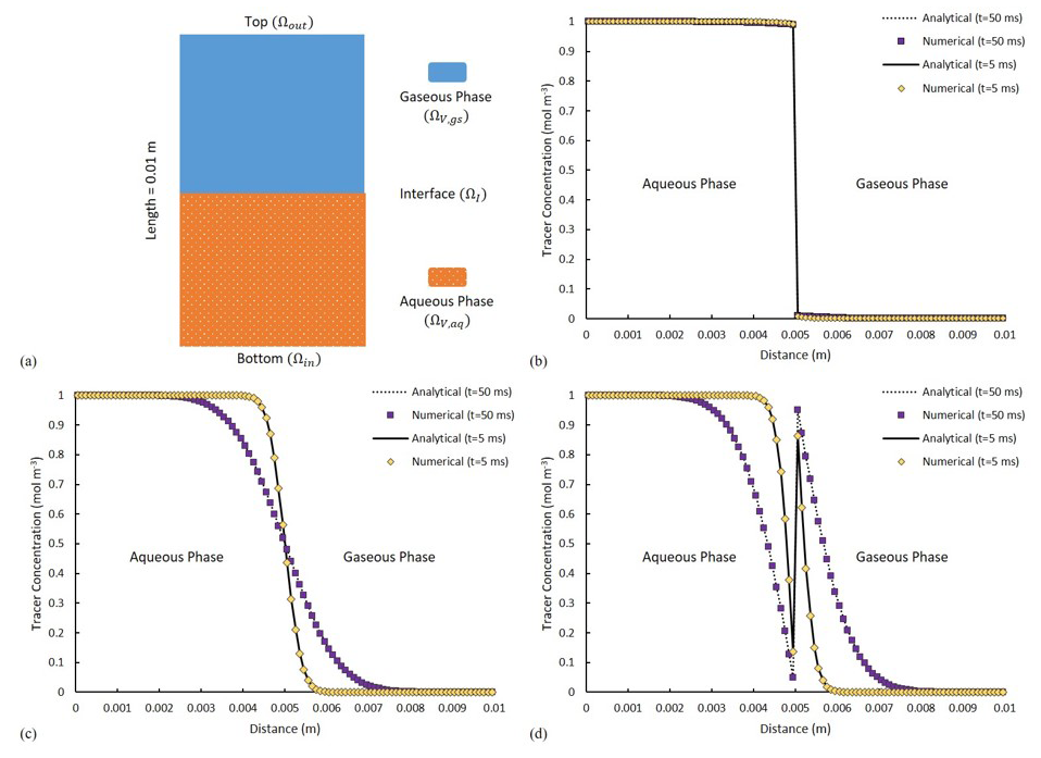
Figure 4 (a) A schematic of the fluid distributions at initial condition. The solid and dotted lines show the analytical solutions, with purple and yellow symbols depicting the numerical solutions. Comparison of the analytical and numerical solutions of tracer distribution at two distinct time points of t₁=5 ms and t₂=50 ms for (b) H =0.01, (c) H =1 and (d) H =100.

3.2 Mass transfer across the fluid–fluid interface

Mass transfer of dissolved species between different phases is particularly of importance for various biogeochemical processes in unsaturated subsurface environments.

Model performance in simulating mass flux across the fluid–fluid interface is validated via a numerical experiment in which two immiscible stationary fluids (an aqueous – α – and a gaseous – β – phase, u=0 in Ω_ϑ) are horizontally (to remove buoyancy effects) residing in a one-dimensional tube of 10 mm length with mesh size of 100 µm. The general partial differential equation (PDE) of Eq. (12) takes the form of a simple diffusive transport as

$$\begin{array}{}\text{(25)}& \begin{array}{rl}& {\displaystyle \frac{\partial C_{\mathrm{tr},i}}{\partial t}}-D_{\mathrm{tr},i}\mathrm{\nabla }\left(C_{\mathrm{tr},i}\right)=\mathrm{0}i=\mathrm{aq},\mathrm{gs}\\ & \mathrm{BC}-\mathrm{1}:C_{\mathrm{tr},\mathrm{aq}}\times H=C_{\mathrm{tr},\mathrm{gs}}\mathrm{in}{\mathrm{\Omega }}_{\mathrm{I}}\\ & \mathrm{BC}-\mathrm{2}:D_{\mathrm{tr},\mathrm{aq}}{\displaystyle \frac{\partial C_{\mathrm{tr},\mathrm{aq}}}{\partial x}}=D_{\mathrm{tr},\mathrm{gas}}{\displaystyle \frac{\partial C_{\mathrm{tr},\mathrm{gs}}}{\partial x}}\mathrm{in}{\mathrm{\Omega }}_{\mathrm{I}},\end{array}\end{array}$$

with C_tr as the concentration of a volatile tracer and D_tr,i as the diffusivity of the tracer in phase i. Each phase is set to occupy half of the total volume (Fig. 4a). The system is initialized with a volatile chemical species of concentration of 1 mol m⁻³ in Ω_ϑ,aq and 0 mol m⁻³ in Ω_ϑ,gs. At the inlet and the outlet boundary, tracer concentration equals that of the nearest solution such that, in a short simulation time, it yields no concentration gradient into or out of the domain. The tendency of the dissolved chemical component to cross the fluid–fluid interface is expressed using a constant Henry coefficient. Tracer diffusivity is set to be $\mathrm{1}\times {\mathrm{10}}^{-\mathrm{5}}$ m² s⁻¹ in both phases. The analytical solution for Eq. (25) can be found in Bird (2002).

Three scenarios with low, neutral and high affinity of the volatile compound towards the gaseous phase are considered with corresponding Henry coefficients of 0.01 (low-volatility, similar to naphthalene), 1 (moderate-volatility, for example, vinyl chloride) and 100 respectively (high-volatility, for example, heptane). For a low value of H (H=0.01 – Fig. 4b), little (almost no) tracer is crossing the interface, while at neutral condition (H=1 – Fig. 4c), tracer diffusion is invariant to the phase it is occupying. Evidently for high values of H (H=100 – Fig. 4d), significant reduction in the tracer amount within the liquid phase can be detected, which is accompanied by a notable change in concentration across the interface. This complies fully with the concentration jump for such highly volatile components between the liquid and the gas phase. The numerical results are ubiquitously identical to the results of the analytical solution (Fig. 4b, c, d). The effect of grid size/resolution is also investigated for this scenario. With 10 times higher grid resolution, the total CPU-elapsed time is increased from ∼650 to ∼3500 s. The concentration profile remains unchanged, but, the average residual of the numerical solution of the concentration field, calculated at the end of the simulation, is increased from $\mathrm{3.1}\times {\mathrm{10}}^{-\mathrm{10}}$ to $\mathrm{6.5}\times {\mathrm{10}}^{-\mathrm{10}}$ (meaning increasing resolution does not necessarily help with numerical convergence).

3.3 Microbial growth and reactive transport

Our modelling framework can parameterize any type of reactions; we put the main focus in this subsection on microbially driven redox transformations (i.e. a type of reactions commonly encountered in soils and other porous media environments) and on the implementation of the corresponding mathematical formulation. To validate our model with a scenario in which bacterial biomass is allowed to evolve (i.e. to grow and to decay), we adapted a conceptual biodegradation scenario from Cirpka and Valocchi (2007) in which a fully water-saturated, two-dimensional channel is subjected to a constant flux of two different components, ED (electron donor, for example, hydrocarbon) and EA (electron acceptor, for example oxygen). The imposed uniform flow field is assumed to be constant over time and only has the x component. The bacteria residing in the channel facilitate the reaction between ED and EA, which can be written in an abstract form as $f_a\mathrm{ED}+f_b\mathrm{EA}\stackrel{\mathrm{biomass}}{⟶}{f}_c$Prod, where biomass is the microbial biomass, Prod is the product(s) (e.g. metabolites such as carbon dioxide), and f_a, f_b and f_c are stoichiometric coefficients. Assuming a double-Monod kinetics for expressing microbial growth and the microbially driven reaction rates, as well as assuming none of the reactants nor products are involved in secondary reactions, the ADRE (Eq. 12) for each chemical species can then be written as

$$\begin{array}{}\text{(26)}& \begin{array}{rl}& {\displaystyle \frac{\partial C_{\mathrm{ED}}}{\partial t}}+\mathbf{u}{\displaystyle \frac{\partial C_{\mathrm{ED}}}{\partial x}}-D_{\mathrm{t}}{\displaystyle \frac{{\partial }^{\mathrm{2}}{C}_{\mathrm{ED}}}{\partial y^{\mathrm{2}}}}=-{\displaystyle \frac{C_{\mathrm{ED}}}{C_{\mathrm{ED}}+K_{\mathrm{ED}}}}\\ & {\displaystyle \frac{C_{\mathrm{EA}}}{C_{\mathrm{EA}}+K_{\mathrm{EA}}}}{\displaystyle \frac{{\mathit{\mu }}_{\max }}{Y}}{f}_a{C}_{\mathrm{bio}}\text{in}{\mathrm{\Omega }}_{\mathit{\vartheta }}\\ & {\displaystyle \frac{\partial C_{\mathrm{EA}}}{\partial t}}+\mathbf{u}{\displaystyle \frac{\partial C_{\mathrm{EA}}}{\partial x}}-D_{\mathrm{t}}{\displaystyle \frac{{\partial }^{\mathrm{2}}{C}_{\mathrm{EA}}}{\partial y^{\mathrm{2}}}}=\\ & -{\displaystyle \frac{C_{\mathrm{ED}}}{C_{\mathrm{ED}}+K_{\mathrm{ED}}}}{\displaystyle \frac{C_{\mathrm{EA}}}{C_{\mathrm{EA}}+K_{\mathrm{EA}}}}{\displaystyle \frac{{\mathit{\mu }}_{\max }}{Y}}{f}_b{C}_{\mathrm{bio}}\text{in}{\mathrm{\Omega }}_{\mathit{\vartheta }}\\ & {\displaystyle \frac{\partial C_{\mathrm{Prod}}}{\partial t}}+\mathbf{u}{\displaystyle \frac{\partial C_{\mathrm{Prod}}}{\partial x}}-D_{\mathrm{t}}{\displaystyle \frac{{\partial }^{\mathrm{2}}{C}_{\mathrm{Prod}}}{\partial y^{\mathrm{2}}}}={\displaystyle \frac{C_{\mathrm{ED}}}{C_{\mathrm{ED}}+K_{\mathrm{ED}}}}\\ & {\displaystyle \frac{C_{\mathrm{EA}}}{C_{\mathrm{EA}}+K_{\mathrm{EA}}}}{\displaystyle \frac{{\mathit{\mu }}_{\max }}{Y}}{f}_c{C}_{\mathrm{bio}}\text{in}{\mathrm{\Omega }}_{\mathit{\vartheta }}\\ & {\displaystyle \frac{\partial C_{\mathrm{bio}}}{\partial t}}={\displaystyle \frac{C_{\mathrm{ED}}}{C_{\mathrm{ED}}+K_{\mathrm{ED}}}}{\displaystyle \frac{C_{\mathrm{EA}}}{C_{\mathrm{EA}}+K_{\mathrm{EA}}}}{\mathit{\mu }}_{\max }{C}_{\mathrm{bio}}\\ & -\mathit{\lambda }{C}_{\mathrm{bio}}\text{in}{\mathrm{\Omega }}_{\mathit{\vartheta }},\end{array}\end{array}$$

where u is the velocity (which has only a constant x-component); D_t is the transverse dispersivity; C_ED, C_EA, C_Met and C_bio are concentrations of ED, EA, Prod and biomass respectively; K_ED and K_EA are half-saturation constants for respective compounds in the biomass growth term; Y is the yield coefficient; μ_max is the maximum bacterial growth rate; and λ is the bacterial decay rate. Using these equations, Cirpka and Valocchi (2007) developed an analytical solution for steady-state conditions, which in the version of Cirpka and Valocchi (2009) is used as reference for the numerical results.

The numerical experiment is designed to have ED and EA, occupying 25 % and 75 % of the inlet respectively, and, simultaneously, invading the domain under a constant uniform velocity field, with concentration of $C_{\mathrm{ED}}^{\mathrm{inlet}}$ and $C_{\mathrm{EA}}^{\mathrm{inlet}}$. In a real-world scenario, this can be seen as a plume of a contaminant (i.e. a hydrocarbon as ED) being carried into the domain within an oxygenated stream, and essentially we are interested in knowing the final concentration/distribution of all biochemical species within the domain. The parameters used in this scenario are summarized in Table 1. Transient reactive transport simulations are performed until a steady state is achieved. For validation, we analyse all concentration profiles along the y axis at a fixed distance of x=2 m and compare them with the analytical solutions. The analytical and numerical results show an almost perfect agreement (Fig. 5b–e).

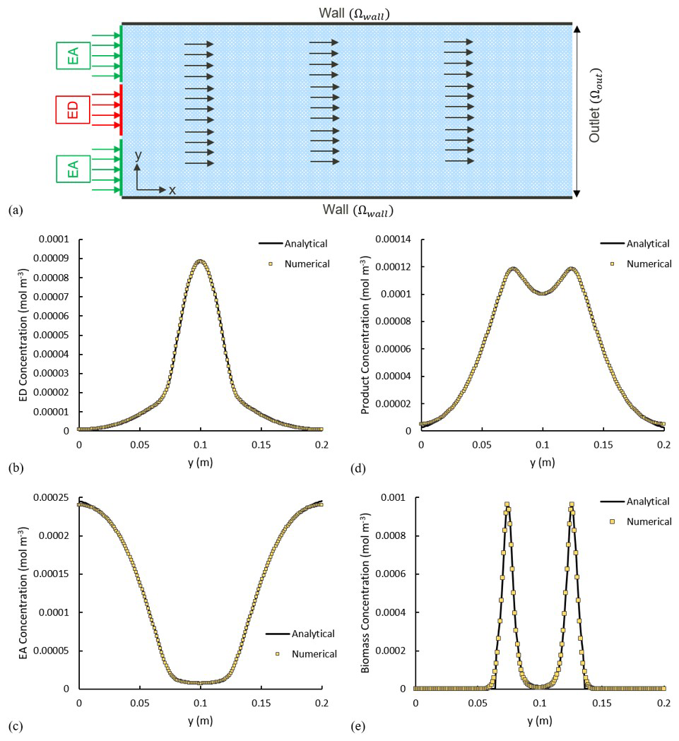
Figure 5 (a) Model setup. The arrows show the direction of the flow field. Solid lines show the analytical solution, and the yellow squares illustrate the numerical results. (b–e) Comparison of the analytical and numerical solutions x=2 m for concentration of (b) electron donor, (c) electron acceptor, (d) product and (e) biomass.

Table 1 Parameter values used for simulating microbial growth.

3.4 Theme: demonstrating model capabilities

The scenarios described above are designed to serve as the sole purpose of creating a baseline for validating the numerical toolbox – simple enough where analytical solutions could exist. Unlike the simplicity introduced in previous sections, simulating soil processes with all of the complexities, though, would require having all the modelling elements to be present. We thus present here a scenario with an unsaturated soil hosting the facultative anaerobic bacteria Agrobacterium tumefaciens, which performs aerobic respiration under oxic conditions but switches to denitrification using nitrate, nitrite or nitric oxide under anoxic conditions (Kampschreur et al., 2012). This example allows us to show our model capabilities, as it involves (1) the actual microstructure of the soil, (2) unsaturated conditions and (3) an enzymatic reaction network with limiting/inhibition terms. The microstructure is obtained via subsampling from a larger µ-CT image with a voxel size of 6 µm (see Supplement). A two-phase simulation is then performed on the voxelized subsample to obtain the fluxes and phase distribution of air and water within the pore space. For this, the entire domain is initially filled with water and subject to injecting air from the top boundary with a constant flux of 0.013 mL h⁻¹. An important note to make here is with a relatively high influx, advection transport acts as the bottleneck for numerical time steps. Hence, reactions are performed at quite a slower pace (i.e. larger time steps roughly estimated around 10 h). This separation of processes helps improve the overall run time of the simulations. Generally, the time step sizes are automatically enforced by the Courant number from the transient advective–diffusive transport equation (with order of 10⁻⁵ s). The biomass is assumed to be non-motile, meaning it sticks to the solid surface and shows no planktonic behaviour. Fluids are allowed to leave the domain from the bottom part (kept at atmospheric pressure), while all the remaining sides are set to be impermeable walls. Once fluid configurations in the domain are stationary, their distribution, along with the velocity profile, is used as a basis for the reactive transport simulations (phase distributions can be found in the Supplement). Using succinate (${\mathrm{C}}_{\mathrm{4}}{\mathrm{H}}_{\mathrm{4}}{\mathrm{O}}_{\mathrm{4}}^{\mathrm{2}-}$) as the organic carbon substrate to be degraded, a metabolic reaction network is constructed with four microbial degradation pathways each following Monod-type kinetics: (1) aerobic respiration with a nitric oxide (NO) inhibitory term; (2) nitrate (NO${}_{\mathrm{3}}^{-}$) reduction; (3) nitrite (NO${}_{\mathrm{2}}^{-}$) reduction; and (4) NO reduction, with having oxygen (O₂) as the inhibitory element for all denitrification conversions (Eq. 27). Also three additional equations are considered for the synthesis of the three different enzymes required for degradation processes (Eq. 28). We consider only one single strain of bacteria (Agrobacterium tumefaciens) which has the benefits of performing both aerobic respiration and denitrification. Bacteria are considered to be non-motile with an initial concentration of 0.25 mol m⁻² and uniformly covering the entire grain surface area. Succinate has its initial concentration in the aqueous phase set at 0.2 mM (0 mM in the gaseous phase), while all other species have their initial concentrations of 0 mM in both aqueous and gaseous phases. The boundary condition for all concentration fields on all boundaries is set to zero gradient, except for the inlet boundary (fully saturated with air), where for oxygen it is set to 0.03567 mM, and for all others it is set to 0 mM. In order to avoid depletion of the nitrate in the system, a nitrate concentration of 0.1 µM (as initial condition) is provided. The complete reaction network can be written as follows (Kampschreur et al., 2012):

$$\begin{array}{}\text{(27)}& \begin{array}{rl}& \text{(a)}{\mathrm{C}}_{\mathrm{4}}{\mathrm{H}}_{\mathrm{4}}{\mathrm{O}}_{\mathrm{4}}^{\mathrm{2}-}+\mathrm{1.2}{\mathrm{O}}_{\mathrm{2}}+\mathrm{1.56}{\mathrm{H}}^{+}+\mathrm{0.44}{\mathrm{NH}}_{\mathrm{4}}^{+}\\ & \to \mathrm{2.2}{\mathrm{CH}}_{\mathrm{1.8}}{\mathrm{O}}_{\mathrm{0.5}}{\mathrm{N}}_{\mathrm{0.2}}+\mathrm{1.8}{\mathrm{CO}}_{\mathrm{2}}+\mathrm{1.68}{\mathrm{H}}_{\mathrm{2}}\mathrm{O}\\ & \text{(b)}{\mathrm{C}}_{\mathrm{4}}{\mathrm{H}}_{\mathrm{4}}{\mathrm{O}}_{\mathrm{4}}^{\mathrm{2}-}+\mathrm{3.23}{\mathrm{NO}}_{\mathrm{3}}^{-}+\mathrm{1.6}{\mathrm{H}}^{+}+\mathrm{0.36}{\mathrm{NH}}_{\mathrm{4}}^{+}\\ & \to \mathrm{1.8}{\mathrm{CH}}_{\mathrm{1.8}}{\mathrm{O}}_{\mathrm{0.5}}{\mathrm{N}}_{\mathrm{0.2}}+\mathrm{3.23}{\mathrm{NO}}_{\mathrm{2}}^{-}+\mathrm{2.2}{\mathrm{CO}}_{\mathrm{2}}\\ & +\mathrm{1.92}{\mathrm{H}}_{\mathrm{2}}\mathrm{O}\\ & \text{(c)}{\mathrm{C}}_{\mathrm{4}}{\mathrm{H}}_{\mathrm{4}}{\mathrm{O}}_{\mathrm{4}}^{\mathrm{2}-}+\mathrm{6.45}{\mathrm{NO}}_{\mathrm{2}}^{-}+\mathrm{8.09}{\mathrm{H}}^{+}+\mathrm{0.36}{\mathrm{NH}}_{\mathrm{4}}^{+}\\ & \to \mathrm{1.8}{\mathrm{CH}}_{\mathrm{1.8}}{\mathrm{O}}_{\mathrm{0.5}}{\mathrm{N}}_{\mathrm{0.2}}+\mathrm{6.45}\mathrm{NO}+\mathrm{2.2}{\mathrm{CO}}_{\mathrm{2}}+\mathrm{5.15}{\mathrm{H}}_{\mathrm{2}}\mathrm{O}\\ & \text{(d)}{\mathrm{C}}_{\mathrm{4}}{\mathrm{H}}_{\mathrm{4}}{\mathrm{O}}_{\mathrm{4}}^{\mathrm{2}-}+\mathrm{6.45}\mathrm{NO}+\mathrm{1.64}{\mathrm{H}}^{+}+\mathrm{0.36}{\mathrm{NH}}_{\mathrm{4}}^{+}\\ & \to \mathrm{1.8}{\mathrm{CH}}_{\mathrm{1.8}}{\mathrm{O}}_{\mathrm{0.5}}{\mathrm{N}}_{\mathrm{0.2}}+\mathrm{3.23}{\mathrm{N}}_{\mathrm{2}}\mathrm{O}+\mathrm{2.2}{\mathrm{CO}}_{\mathrm{2}}\\ & +\mathrm{1.92}{\mathrm{H}}_{\mathrm{2}}\mathrm{O}.\end{array}\end{array}$$

Several assumptions are made for preparing the kinetics of the reactions: (1) reaction rates are limited by the maximum specific uptake rate of succinate and are hence independent of its concentration (Beun et al., 2000); (2) a sufficient amount of buffer is added to the solution to keep the pH level constant; (3) three nitrogen reductase enzymes (ξ_sat, NOR for NO reduction, ξ_sat, NIR for nitrite reduction and ξ_sat, NAP for nitrate reduction) can have saturation values varying between 0 (i.e. non-existing) and 1 in a bacterial cell; and (4) inhibitory oxygen limits the reduction of NO, ${\mathrm{NO}}_{\mathrm{2}}^{-}$ and ${\mathrm{NO}}_{\mathrm{3}}^{-}$. Reaction rates are designed to have a dependency on the enzymes' level and biomass concentration with proper limiting/inhibiting terms. Equation (12) is used to describe the evolution of each biochemical species. The final system of advective–diffusive–reactive equations is adapted from Kampschreur et al. (2012):

$$\begin{array}{}\text{(28)}& \begin{array}{rl}& {\displaystyle \frac{\partial C_i}{\partial t}}+\mathrm{\nabla }\cdot \left(C_i\mathbf{u}\right)=-\mathrm{\nabla }\cdot \left(D_i\mathrm{\nabla }{C}_i-D_i{\displaystyle \frac{\mathrm{1}-H_i}{\mathit{\alpha }+\left(\mathrm{1}-\mathit{\alpha }\right)H_i}}{C}_i\mathrm{\nabla }\mathit{\alpha }\right)\\ & +R_i,i=\mathrm{suc},{\mathrm{O}}_{\mathrm{2}},{\mathrm{NO}}_{\mathrm{3}}^{-}{\mathrm{NO}}_{\mathrm{2}}^{-},\mathrm{NO},{\mathrm{N}}_{\mathrm{2}}\mathrm{O}\mathrm{in}{\mathrm{\Omega }}_{\mathit{\vartheta }}\\ & R_{\mathrm{suc}}=-(r_{\mathrm{suc},{\mathrm{O}}_{\mathrm{2}}}+r_{\mathrm{suc},\mathrm{NAP}}+r_{\mathrm{suc},\mathrm{NIR}}+r_{\mathrm{suc},\mathrm{NOR}})\\ & R_{{\mathrm{O}}_{\mathrm{2}}}=-\mathrm{1.2}{r}_{\mathrm{suc},{\mathrm{O}}_{\mathrm{2}}}\\ & R_{{\mathrm{NO}}_{\mathrm{3}}^{-}}=-\mathrm{3.23}{r}_{\mathrm{suc},\mathrm{NAP}}\\ & R_{{\mathrm{NO}}_{\mathrm{2}}^{-}}=\mathrm{3.23}{r}_{\mathrm{suc},\mathrm{NAP}}-\mathrm{6.45}{r}_{\mathrm{suc},\mathrm{NIR}}\\ & R_{\mathrm{NO}}=\mathrm{6.45}{r}_{\mathrm{suc},\mathrm{NIR}}-\mathrm{6.45}{r}_{\mathrm{suc},\mathrm{NOR}}\\ & R_{{\mathrm{N}}_{\mathrm{2}}\mathrm{O}}=\mathrm{3.23}{r}_{\mathrm{suc},\mathrm{NOR}}\\ & r_{\mathrm{suc},{\mathrm{O}}_{\mathrm{2}}}={\mathit{\mu }}_{\max }{C}_{\mathrm{bio}}{\displaystyle \frac{C_{{\mathrm{O}}_{\mathrm{2}}}}{K_{{\mathrm{O}}_{\mathrm{2}}}\left(\mathrm{1}+\frac{C_{\mathrm{NO}}}{K_{\mathrm{I},\mathrm{NO},{\mathrm{O}}_{\mathrm{2}}}}\right)+C_{{\mathrm{O}}_{\mathrm{2}}}}}\\ & r_{\mathrm{suc},\mathrm{NAP}}={\mathit{\mu }}_{\max }{C}_{\mathrm{bio}}{\mathit{\xi }}_{\mathrm{sat},\mathrm{NAP}}{\displaystyle \frac{C_{{\mathrm{NO}}_{\mathrm{3}}}}{K_{{\mathrm{NO}}_{\mathrm{3}}}+C_{{\mathrm{NO}}_{\mathrm{3}}}}}\\ & {\displaystyle \frac{K_{\mathrm{I},{\mathrm{O}}_{\mathrm{2}},\mathrm{NAP}}^{\mathrm{nNAP}}}{K_{\mathrm{I},{\mathrm{O}}_{\mathrm{2}},\mathrm{NAP}}^{\mathrm{nNAP}}+C_{{\mathrm{O}}_{\mathrm{2}}}^{\mathrm{nNAP}}}}\\ & r_{\mathrm{suc},\mathrm{NIR}}={\mathit{\mu }}_{\max }{C}_{\mathrm{bio}}{\mathit{\xi }}_{\mathrm{sat},\mathrm{NIR}}{\displaystyle \frac{C_{{\mathrm{NO}}_{\mathrm{2}}}}{K_{{\mathrm{NO}}_{\mathrm{2}}}+C_{{\mathrm{NO}}_{\mathrm{2}}}}}\\ & {\displaystyle \frac{K_{\mathrm{I},{\mathrm{O}}_{\mathrm{2}},\mathrm{NIR}}^{\mathrm{nNIR}}}{K_{\mathrm{I},{\mathrm{O}}_{\mathrm{2}},\mathrm{NIR}}^{\mathrm{nNIR}}+C_{{\mathrm{O}}_{\mathrm{2}}}^{\mathrm{nNIR}}}}\\ & r_{\mathrm{suc},\mathrm{NOR}}={\mathit{\mu }}_{\max }{C}_{\mathrm{bio}}{\mathit{\xi }}_{\mathrm{sat},\mathrm{NOR}}{\displaystyle \frac{C_{\mathrm{NO}}^{\mathrm{2}}}{{\left[C_{\mathrm{NO}}\left(\mathrm{1}+\frac{C_{\mathrm{NO}}}{K_{\mathrm{I},\mathrm{NO}}}\right)+K_{\mathrm{NO}}\right]}^{\mathrm{2}}}}\\ & {\displaystyle \frac{K_{\mathrm{I},{\mathrm{O}}_{\mathrm{2}},\mathrm{NOR}}}{K_{\mathrm{I},{\mathrm{O}}_{\mathrm{2}},\mathrm{NOR}}+C_{{\mathrm{O}}_{\mathrm{2}}}}}\\ & {\displaystyle \frac{\mathrm{d}{\mathit{\xi }}_{\mathrm{sat},\mathrm{NAP}}}{\mathrm{d}t}}={\mathit{\nu }}_{\mathrm{m},\mathrm{NAP}}{\displaystyle \frac{C_{{\mathrm{NO}}_{\mathrm{3}}}}{K_{{\mathrm{NO}}_{\mathrm{3}},\mathrm{NAP}}+C_{{\mathrm{NO}}_{\mathrm{3}}}}}\\ & {\displaystyle \frac{K_{\mathrm{I},{\mathrm{O}}_{\mathrm{2}},\mathrm{NAP}}}{K_{\mathrm{I},{\mathrm{O}}_{\mathrm{2}},\mathrm{NAP}}+C_{{\mathrm{O}}_{\mathrm{2}}}}}\left(\mathrm{1}-{\mathit{\xi }}_{\mathrm{sat},\mathrm{NAP}}\right)\\ & {\displaystyle \frac{\mathrm{d}{\mathit{\xi }}_{\mathrm{sat},\mathrm{NIR}}}{\mathrm{d}t}}={\mathit{\nu }}_{\mathrm{m},\mathrm{NIR}}{\displaystyle \frac{C_{{\mathrm{NO}}_{\mathrm{2}}}}{K_{{\mathrm{NO}}_{\mathrm{2}},\mathrm{NIR}}+C_{{\mathrm{NO}}_{\mathrm{2}}}}}\left(\mathrm{1}-{\mathit{\xi }}_{\mathrm{sat},\mathrm{NIR}}\right)\\ & {\displaystyle \frac{\mathrm{d}{\mathit{\xi }}_{\mathrm{sat},\mathrm{NOR}}}{\mathrm{d}t}}={\mathit{\nu }}_{\mathrm{m},\mathrm{NOR}}{\displaystyle \frac{C_{\mathrm{NO}}}{K_{\mathrm{NO},\mathrm{NOR}}+C_{\mathrm{NO}}}}\left(\mathrm{1}-{\mathit{\xi }}_{\mathrm{sat},\mathrm{NOR}}\right)\\ & {\displaystyle \frac{\mathrm{d}{C}_{\mathrm{bio}}}{\mathrm{d}t}}=\mathrm{2.2}{r}_{\mathrm{suc},{\mathrm{O}}_{\mathrm{2}}}+\mathrm{1.8}\left(r_{\mathrm{suc},\mathrm{NAP}}+r_{\mathrm{suc},\mathrm{NIR}}\right.\\ & \left.+r_{\mathrm{suc},\mathrm{NOR}}\right).\end{array}\end{array}$$

The full list of modelling parameters used for this study can be found in the Supplement.

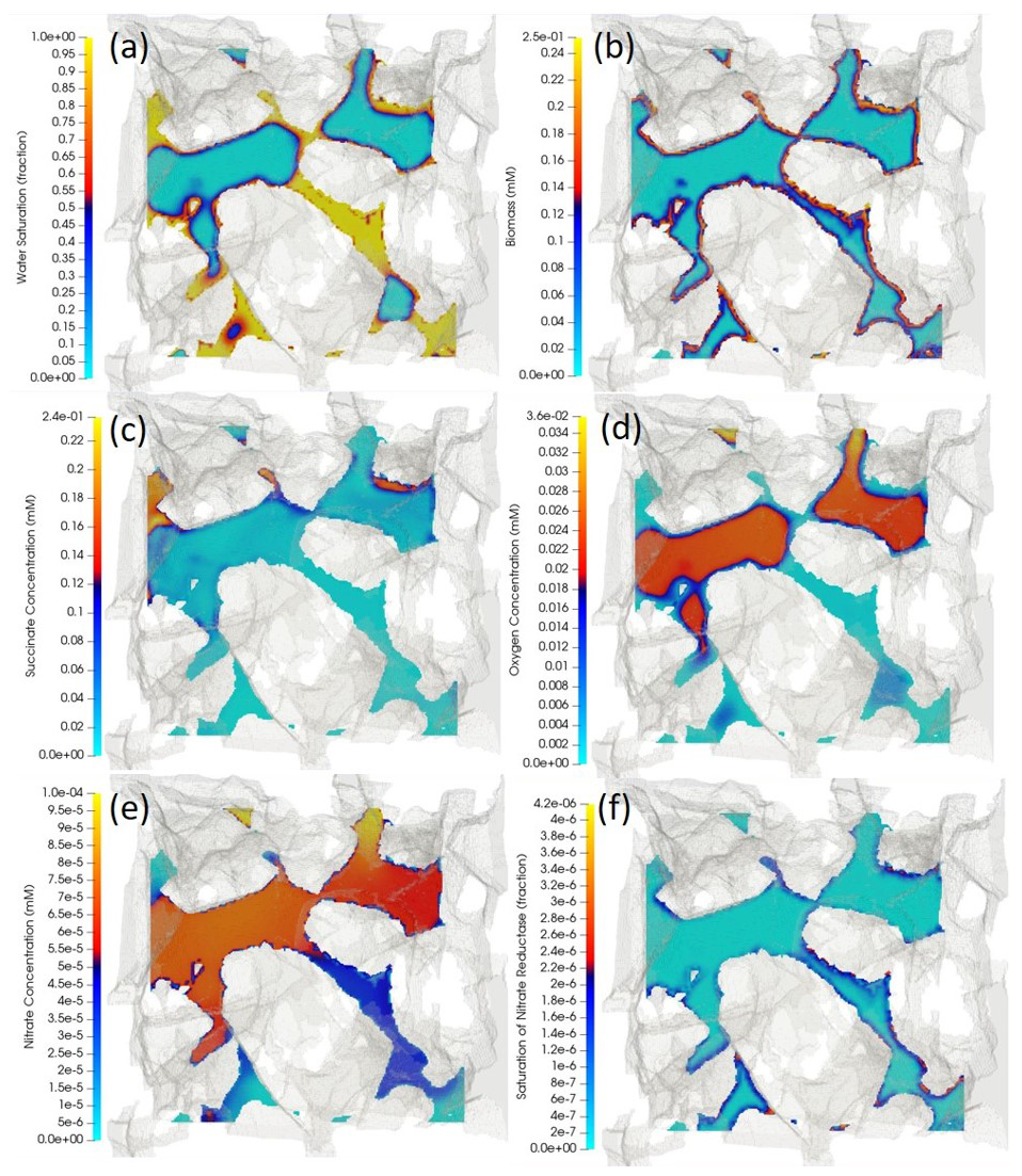
Figure 6 Cross-sectional view of the three-dimensional porous medium. The cutting plane is arbitrary, cutting through the middle of the porous structure, meaning at some locations that the phases are continuous perpendicular to the plane. The opaque greyish background represents the 3D porous structure that is extracted and digitized from a µ-CT image. The coloured surfaces are obtained by running a cutting plane through the middle of the sample and perpendicular to the z axis. The distribution of (a) water-content fraction (i.e. water-volume fraction), (b) biomass, (c) succinate, (d) oxygen, (e) nitrate and (f) nitrate reductase enzyme are respectively depicted, with yellow indicating the highest value and light blue the lowest value. Air in the non-wetting phase is expected to fill in the middle of the pore space where capillary pressure is lower, while water, in the wetting phase, is expected to occupy the corners (a). A high-volatility constant for oxygen causes there to be higher concentrations of oxygen in the air compared to those of the aqueous phase adjacent to the water–air interface.

Reactive transport simulations were performed until a quasi-steady state was achieved. This was characterized by all chemical species concentrations reaching a steady state, as determined by the degradation activity of the given distribution of microorganisms. Since microbial growth takes place at much larger timescales than the pore-scale transport processes, no significant growth takes place during the simulated time period, and results shown are nearly identical to the initial conditions. Simulation results show that the presence of air in this two-phase system affects the distribution of biochemical species. Air, in the non-wetting phase, occupies the central part of the pore space, while the aqueous phase is expected to cover the corners and crevices (Fig. 6a). For oxygen with $H_{{\mathrm{O}}_{\mathrm{2}}}=\mathrm{31}$, a higher concentration is observed in the air compared to that of the adjacent aqueous phase (Fig. 6d). An analysis of how the volatility of a tracer compound may affect its residence time in the porous medium is given in the Supplement. Since the biomass is only present on the grain surfaces (Fig. 6b), oxygen, nitrate and succinate deplete as the microbially mediated reactions only occur at these micro-locations. Fresh oxygen and nitrate thus need to diffuse from the bulk (either from the aqueous phase or the air) to the reactive sites. The regions with high (i.e. not degraded) succinate concentrations are compatible with low concentration regions of oxygen and nitrate; i.e. the reactions are limited by the bioavailable oxygen and nitrate (Fig. 6b–e). Finally, all three enzymes have an increased abundance in anaerobic regions with an active biomass (saturation map of nitrate reductase enzyme is shown in Fig. 6e). While the saturation of nitrate reductase enzyme grows linearly with time (until 0.25 s), the rate at which the nitrite and NO reductase enzymes (ξ_sat, NIR and ξ_sat, NOR respectively) grow is rather slow for the very beginning of the simulation (until ∼0.2 s), but it surges exponentially afterward. A spatially integrated assessment of the degradation processes showed that for the presented example, 99 % of the total succinate degradation is attributed to aerobic respiration, while a trivial amount is attributed to the three anaerobic processes (nitrate reduction, nitrite reduction and NO reductions).

The presented results highlight the ability of the model to combine a high-resolution simulation of multi-phase flow and transport processes with the simulation of complex biogeochemical processes. This allows for a realistic simulation of the pore-scale distribution of reactive processes and for the derivation of an accurate aggregated description of these processes.

As it can be seen from Fig. 6, our model can be used (among other options) to identify clusters in which succinate is most and least depleted. This would ease the process of analysing the results by isolating the parameters that are boosting/limiting the degradation of the carbon source. A 3D visualization of the oxygen and succinate distributions can be found in Golparvar (2022).

4 Conclusion and future remarks

In this paper, we have presented a newly developed modelling framework for simulating reactive transport processes in real porous soil structures obtained from µ-CT images under unsaturated conditions. The successful application of various benchmark test showed the model's accuracy in the simulation of (1)  the movement of water and air phase in variably saturated conditions via the enhanced algebraic volume-of-fluid method (Raeini et al., 2012) coupled with the Navier–Stokes equation; (2) the transport of different species in both phases by the full advective–diffusive transport equation; and finally (3) use of the operator splitting technique, an arbitrary set of biogeochemical reactions solved externally by the Biogeochemical Reaction Network Simulator and communicated back into the main solver.

The presented model provides a novel and unique combination of pore-scale simulations of two-phase flow, transport of dissolved and volatile species, and their reactive transformations. This makes it an accurate and powerful tool for the simulation of soil systems or other unsaturated porous media and of the reactive transport processes therein. While developed with the aim for simulating biogeochemical processes in soils, the model is equally applicable for simulating other abiotic reactive processes coupled to the dynamics of flow and transport in variably saturated pore structures of arbitrary geometry. Our modelling framework is properly designed for simulating biogeochemical processes such as carbon–nitrogen–sulfur–phosphorus cycles in soil as well as mixing and migration of contaminants in both unsaturated soil and water aquifers. It comes with the benefit of explicit recognition of the soil structure (i.e. using the 3D structure as close to the original shape as possible with the least number of simplifications/modifications), phase dynamics/distributions, and the capability of designing the complete redox reactions necessary for a given process in a straightforward fashion. It is best suitable for running pre-pilot tests as feasibility scenarios where the stakes for the success of the project are high. Also, our model provides the best tool for designing hypothetical experiments that are hard (if not impossible) to implement experimentally (e.g. a specific distribution of biomass–reactants within the domain, or variation of specific properties of reactive compound and/or the porous matrix). Furthermore, the high-resolution modelling results provided by this model support the upscaling of reactive transport process description from the pore to the Darcy scale and from the process to the observation scale respectively.

Although the current version of our numerical model is already covering a wide range of biophysiochemical properties of the soil constituents, for having a more realistic representation of multiphase, multicomponent reactive transport in partially saturated porous media, a few more factors still might be considered in future developments of the model: (1) shrinkage/expansion of the air/aqueous phase due to mass transfer of chemical species across the fluid–fluid interface; (2) the accounting of gas compressibility by adding an equation of state for tracking changes of air volume/density under flowing conditions; (3) translation of accumulated biomass on the grain surfaces into new flow-resistance components, which would potentially change the velocity streamlines (i.e. bioclogging); (4) changes of the grain surface structures and of the associated solid–liquid interface due to mineral precipitation/dilution or due to accumulation/depletion of solid organic material; (5) chemotactic behaviour of the microbial species; and (6) osmotic forces and electro-migration. Due to the modular structure of P3D-BRNS, such features can be relatively easily included in future upgrades of our model.